CTSyn: A Foundational Model for Cross Tabular Data Generation

Abstract

Generative Foundation Models (GFMs) have produced synthetic data with remarkable quality in modalities such as images and text. However, applying GFMs to tabular data poses significant challenges due to the inherent heterogeneity of table features. Existing cross-table learning frameworks are hindered by the absence of both a generative model backbone and a decoding mechanism for heterogeneous feature values. To overcome these limitations, we introduce the Cross-Table Synthesizer (CTSyn), a diffusion-based foundational model tailored for tabular data generation. CTSyn introduces three major components: an aggregator that consolidates heterogeneous tables into a unified latent space; a conditional latent diffusion model for sampling from this space; and type-specific decoders that reconstruct values of varied data types from sampled latent vectors. Extensive testing on real-world datasets reveals that CTSyn not only significantly outperforms existing table synthesizers in utility and diversity, but also uniquely enhances performances of downstream machine learning beyond what is achievable with real data, thus establishing a new paradigm for synthetic data generation.

1 Introduction

Generative Foundation Models (GFMs) have revolutionized fields such as Computer Vision (CV) and Natural Language Processing (NLP)[1, 2, 3, 4, 5, 6]. Trained on vast datasets [7, 8, 9] and with versatile model backbones [10, 11], these models excel across a diverse range of domains and tasks. They can generate valuable synthetic training examples to boost performances of various downstream applications [12, 13, 14, 15, 16].

GFMs also hold immense potential for generating tabular data, a modality integral to core real-world applications [17, 18, 19]. Despite the ubiquity of tables, modeling often encounters a shortage of high-quality samples. Although tabular data synthesizers have increasingly gained attention [20, 21, 22], they bring little performance gains in downstream models [23, 24].This limitation stems from a fundamental constraint: literally synthesizers cannot add information not included in the original training data. Tabular GFMs has the potential of overcoming that limitation by leveraging more diverse pre-training data.

Despite such opportunities, the implementation of tabular GFMs remains particularly challenging and largely overlooked, due to the heterogeneity between column structures, features sets and ranges of values [25, 26, 18, 27, 28, 29]. Existing methods for transferable tabular learning either model tables with language models [28, 30, 31, 32], or attempt to learn a unified latent space across datasets [30, 25, 27, 33]. They neither possess generative capability, nor include a unified decoding mechanism that reconstructs heterogeneous table values from row-level representations.

In response to all these limitation, we propose CTSyn, a foundation model framework specifically designed for the generation of heterogeneous tables. CTSyn has the following main components:

• Unified Table Representation: We developed a unified aggregator that tokenizes and embeds heterogeneous table rows, and projects them into a unified latent space. Utilizing self-supervised contrastive learning, regularized by magnitude-aware loss, this approach enhances the preservation of numerical information and facilitates the training of models across tabular formats, thereby overcoming the barrier of data-specific structural needs.

• Generative Foundation Model: Our versatile conditional diffusion model backbone efficiently samples from unified latent spaces, allowing for improved flexibility and applicability across various tabular domains without the need for domain-specific adaptations.

• Data Type-specific Decoder: We trained separate decoder networks that extract column values from latent row embeddings be it numerical values or refined representations of categorical levels. This modular approach in decoding allows us to accommodate different output formats and loss functions tailored to specific column types, effectively eliminating the constraints imposed by traditional data-specific output schemas.

Through extensive experiments with real-world datasets, we demonstrate that CTSyn extends the pre-train/fine-tuning paradigm to the tabular data generation and sets a new benchmark, surpassing the existing State-Of-The-Art (SOTA). Crucially, by effectively leveraging prior knowledge, our model unlocks unprecedented potential in synthetic tabular data generation.

2 Related Work

2.1 Table Representation Learning

Self-supervised learning can significantly enhance the informativeness of representations for various downstream tasks [34, 35, 36, 37]. In the tabular domain, methods like VIME [38] train an encoder using a combination of supervised reconstruction loss and mask-array prediction loss, and SCARF [39] employs contrastive loss by utilizing randomly corrupted feature vectors as positive pairs. Subtab [40] and SSP [41] integrates contrastive and reconstruction losses. However, these approaches do not produce transferable representations across tables as they rely on data-specific feature encoding and structures. Xtab [27] and TabRet [25] introduce transformer-based backbones with separate data-specific featurizer or projection heads for each downstream task. These models achieve transferability at the expense of high model complexity.

Pre-trained Language Models (PLMs) can be used to unify representation dimensions of heterogeneous features. TransTab [30] extends Subtab’s methodology by tokenizing and then encoding column names and categories, creating a latent space that can be shared across tables. Combining tokenization with masked-value-prediction objective, transformer-based models can be trained to perform predictive task across tables [28, 42, 43, 32]. However, such methods include neither a generative model backbone, nor a fixed-dimensional row representation and decoding strategy that could be integrated with other generative model.

Another line of research involving PLMs converts tabular features to sentences and model regression/classification problems as NLP tasks [44, 31, 45, 46, 47, 48]. Despite enabling transfer learning, these methods face challenges with accurately modeling continuous values and tend to overlook the intrinsic structural properties of tables [29].

2.2 Synthetic Tabular Data Generation

Synthetic Tabular Data Generation(STDG) has long been studied by statisticians [49, 50, 51]. Recent success of deep generative models significantly advanced its boundary [52, 53, 54]. In particular, CTGAN [20] combines conditional Generative Adversarial Network(GAN) and model-speicif normalization to model highly imbalanced and non-Gaussian columns. CtabGAN+[55, 56] proposed a solution for mixed-type and long-tailed variable problems. Autodiff [57] and Tabsyn [58] used a combination of latent-diffusion and data-specific autoencoder structure, which is the most similar work to ours but missing the critical transferable encoding/decoding ability. TabDDPM [21] achieved the current state-of-the-art in tabular generation with separate diffusion process for numerical and categorical columns. Some models also synthesizes data with Differential Privacy guarantee [59, 60, 22] Despite their effectiveness in modeling column distributions, none of the above methods is able to effectively boost the training of machine learning models with synthesized data, greatly limiting their usage in data augmentation [24].

GReaT [45] and Tabula [61] generate tables with PLMs, by treating tables rows as natural language text. Despite showing evidences of transferrability, they do not consider cross-table pre-training and generation, introduce risk of producing out-of-bound examples due to their unconstrained sampling of output token, and face the well-known challenge of modeling numeracy in discrete token space [62].

3 Methodology

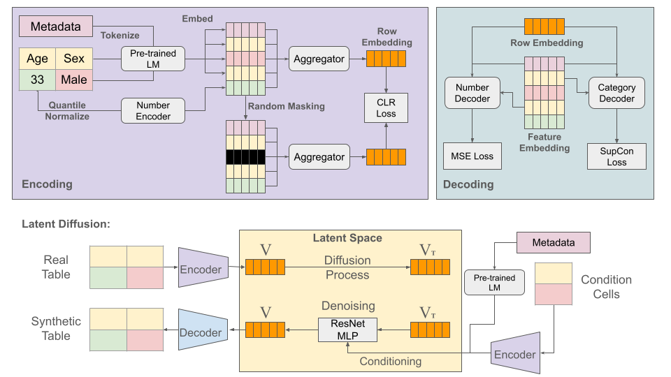
Figure 1: Overview of the proposed framework.

In this section, we outline CTSyn, our solutions to the challenges involved in creating a tabular GFM. Figure 1 provides an overview of the proposed framework.

3.1 Feature Embedding

Let a row in a mixed-type table be $\bm{x}=[c_{1},x_{1},c_{2},x_{2},\ldots,c_{D},x_{D}]$, where $c_{i}$ for $i=1,2,\ldots,D$ are the feature names, $x_{i}$ for $i=1,2,\ldots,D$ are the feature values which can be either numerical or categorical, $D$ denotes the number of features in this row. Let $m$ be the text metadata describing the context of the table.

To enable the transfer of knowledge across tables, a unified representation must preserve all such information. Since dimensions differ across variable types, we tokenize and encode them into vectors of the same dimension. First, we consolidate all text metadata, column names, and categories, ensuring all integer class labels and abbreviations are converted to complete text reflecting their original meanings. Then, we create embeddings as follows:

$$e_{m} =\textbf{LM}(m),\quad e_{c_{i}}=\textbf{LM}(c_{i}),$$

$$e_{x_{i}} =\begin{cases}\textbf{LM}(x_{i})&\text{if }x_{i}\text{ is categorical},\\ \textbf{AE}_{\text{enc}}(\text{Quantile}(x_{i}))&\text{if }x_{i}\text{ is numerical}\end{cases}$$

where LM is a pre-trained language model for text encoding, which will only be called once for each unique category/column name. Quantile is the quantile transformer [63] fitted on $d$ that transforms numerical values to a standard uniform distribution. This improves the modeling of numbers by aligning their ranges and mitigating outliers. $\textbf{AE}_{\text{enc}}$ represents the encoder part of a fully connected autoencoder pre-trained on samples from $\text{Uniform}(0,1)$ (see Appendix Section B), ensuring that quantile-transformed numbers are embedded into the same dimensional space as the language model embeddings while preserving their relative numeracy.

Finally, we interleave all embeddings as a sequence:

$$\bm{E}=[e_{m},e_{c_{1}},e_{x_{1}},e_{c_{2}},e_{x_{2}},\ldots,e_{c_{D}},e_{x_{D}}]\in\mathbb{R}^{(2D+1)\times M_{\text{LM}}},$$ (1)

where $M_{\text{LM}}$ is the dimension of the language model embeddings.

3.2 Embedding Aggregator

We train an aggregator neural network $f(\bm{E})$ to compress a sequence of embeddings into a fixed-dimension latent vector $\bm{v}\in\mathbb{R}^{M_{\text{agg}}}$, where $M_{\text{agg}}$ is the dimension of the learned latent space.

For each row $\bm{x_{i}}$, we create a set of $K+1$ embedding sequences $s_{i}=\{\textbf{E}_{i}^{1},\textbf{E}_{i}^{2},\ldots,\textbf{E}_{i}^{K+1}\}$. $\textbf{E}_{i}^{1}$ is the embedding of all row elements according to Equation 3.1, and the remaining sequences are created by randomly selecting 50% of features in $\bm{x_{i}}$, masking their value embeddings in $\textbf{E}_{i}^{1}$ with a fixed value of $-1$, while retaining the feature names. The aggregator is then trained using a self-supervised contrastive loss:

$$L_{\text{con}}=-\sum_{i=1}^{B}\sum_{k=1}^{K+1}\sum_{k^{\prime}\neq k}^{K+1}\log\frac{\exp(\psi(\bm{v}_{i}^{k},\bm{v}_{i}^{k^{\prime}})/\tau)}{\sum_{j=1}^{B}\sum_{k^{\ast}=1}^{K}\exp(\psi(\bm{v}_{i}^{k},\bm{v}_{j}^{k^{\ast}})/\tau)},$$

where $\bm{v}_{i}^{k}=f(\bm{E}_{i}^{k})$ is the compressed embedding of the $k$th embedding sequence of the $i$th row, $B$ is the batch size, $\psi(\cdot,\cdot)$ is the cosine similarity, and $\tau$ is the temperature constant for numerical stability.

To preserve the relative magnitudes of numerical values within the embeddings, we also modify the Magnitude-Aware Triplet Loss [32]. For each embedding $\bm{v}_{i}$, we randomly select two other embeddings $\bm{v}_{j}$ and $\bm{v}_{k}$ from the batch, ensuring $i\neq j\neq k$. We define the loss as:

$$L_{\text{mag}}=\max\left(\|f(\bm{v}_{i})-f(\bm{v}_{j})\|-\|f(\bm{v}_{i})-f(\bm{v}_{k})\|+m(\bm{v}_{i},\bm{v}_{j},\bm{v}_{k}),0\right),$$

$$m(\bm{v}_{i},\bm{v}_{j},\bm{v}_{k})=\frac{|x_{i,d}-x_{k,d}|-|x_{i,d}-x_{j,d}|}{\text{range}(d)},\quad\text{s.t.}\ |x_{i,d}-x_{k,d}|>|x_{i,d}-x_{j,d}|,$$

where $x_{i,d}$, $x_{j,d}$, and $x_{k,d}$ are the numerical values of a selected numerical column $d$ for rows $i$, $j$, and $k$, respectively. Each epoch, one numerical column is uniformly selected for this loss calculation.

The combined training loss for the aggregator is $L_{\text{aggregator}}=L_{\text{con}}+\lambda L_{\text{mag}},$ where $\lambda=2$ is a weighting constant for the magnitude-aware loss selected by cross-validation. With this combination of masking and contrastive learning, the model learns to represent feature information as well as correlation between features as it is forced to infer closeness of masked features based on available feature values.

3.3 Conditional Diffusion Model for Latent Vector Generation

We employ a conditional Gaussian diffusion model to sample from learned latent distributions of tables. The forward and reverse processes of the model are characterized by Gaussian distributions:

$$q(v_{t}\mid v_{t-1}):=\mathcal{N}\left(v_{t};\sqrt{1-\beta_{t}}v_{t-1},\beta_{t}\mathbf{I}_{M_{\text{agg}}}\right)$$

$$q(v_{T}):=\mathcal{N}(v_{T};\mathbf{0},\mathbf{I}_{M_{\text{agg}}})$$

$$p_{\theta}(v_{t-1}\mid v_{t},y):=\mathcal{N}\left(v_{t-1};\mu_{\theta}(v_{t},y,t),\Sigma_{\theta}(v_{t},y,t)\right)$$

In the main text, $y$ is a conditioning latent vector with dimension $M_{\text{LM}}$. The variance $\Sigma_{\theta}(v_{t},y,t)$ is diagonal with a constant scalar $\sigma_{t}$. For each sample $\bm{v_{i}}$, the corresponding condition $y_{i}$ is formed by the table context embedding $e_{m}$. We report performance of generation conditioned on both table metadata and feature values in appendix section G

The mean $\mu_{\theta}(v_{t},y,t)$ is calculated using:

$$\mu_{\theta}(v_{t},y,t)=\frac{1}{\sqrt{\alpha_{t}}}\left(v_{t}-\frac{\beta_{t}}{\sqrt{1-\bar{\alpha}_{t}}}\epsilon_{\theta}(v_{t},y,t)\right)$$

where $\alpha_{t}:=1-\beta_{t}$ and $\bar{\alpha}_{t}:=\prod_{i=1}^{t}\alpha_{i}$ represent the noise schedule parameters. The function $\epsilon_{\theta}(v_{t},y,t)$ estimates the "ground truth" noise component for the noisy data sample $v_{t}$.

The objective function is simplified to:

$$L_{\text{simple},t}=\mathbb{E}_{v_{0},\epsilon,t}\left[\|\epsilon-\epsilon_{\theta}(v_{t},y,t)\|^{2}\right]$$

3.4 Type-Specific Decoder

Training data-specific table decoders can significantly increase model complexity and elevate the risk of overfitting, particularly when dealing with smaller downstream datasets. Thus, we train type-specific decoders that reconstruct the original values for one cell at a time. To reconstruct the value of a column with name $c_{i}$ in row $x_{i}$ with table metadata $m$, the input to the decoders $H$ is the concatenation of embeddings $[e_{m},e_{c_{i}},v_{i}]$. This concatenation uniquely represents the value for each cell, allowing the decoder to perform accurate reconstruction. We focus on two main data types: categorical and numerical, though this framework can be seamlessly extended to various data types.

Categorical Decoder: Categorical levels vary in sets and textual representations across tables, making decoding one-hot vectors with cross-entropy loss infeasible. Decoding categories as text strings also risks generating unseen columns and losing column structures in categories. Inspired by contrastive-based classification methods in computer vision tasks [64], we train the categorical decoder $H_{\text{cat}}(e_{m},e_{c_{i}},f(E_{i}))\in\mathbb{R}^{M^{\text{dec}}}$ as a projector that maps embeddings of row elements into a cell-level latent space, where cells with the same categories are clustered together.

For each row $\bm{x_{i}}$, we create a set of $K=2$ embeddings $\{E_{i}^{1},E_{i}^{2}\}$. $E_{i}^{1}$ is the embedding of all its elements according to Equation 3.1, and $E_{i}^{2}$ is created by masking the value embedding features in $\bm{x_{i}}$ corresponding to $d$ with a fixed value of $-1$, while retaining the feature names. The presence of an embedding with the actual value absent enforces the model to learn to fill in the missing value based on available values, implicitly preserving the correlation between columns.

We apply the following supervised contrastive loss:

$$L_{\text{cat},d}=-\sum_{i=1}^{B}\sum_{j=1}^{B}\sum_{k=1}^{K}\sum_{k^{\prime}=1}^{K}\mathbf{1}_{\{x_{j,d}=x_{i,d}\}}\log\left(\frac{\exp\psi(z_{i,d}^{k},z_{j,d}^{k^{\prime}})}{\sum_{j^{\ast}=1}^{B}\sum_{k^{\ast}=1}^{K}\mathbf{1}_{\{x_{j^{\ast},d}\neq x_{i,d}\}}\exp\psi(z_{i,d}^{k},z_{j^{\ast},d}^{k^{\ast}})}\right),$$

where $z_{i,d}^{k}=H_{\text{cat}}([e_{m},e_{c_{i}},f(E_{i})])$ is the output of the categorical decoder for the $k$th view of column $d$ in row $i$, and $\mathbf{1}_{\{\cdot\}}$ is the indicator function. This contrastive learning ensures that representations of cells with the same categories are clustered together.

For reconstructing column $d$ for row $i$, we first produce $z_{p,d}=H_{\text{cat}}(e_{m},e_{c_{d}},f([e_{m},e_{c_{d}},e_{p})])$ for each unique category $p$ in $d$, which are considered anchor embeddings of different categories. We then assign the category whose embedding has with the highest cosine similarity to the reconstructed cell embedding $z_{i,d}$.

Numerical Decoder: For decoding numerical values, we employ the numerical decoder $H_{\text{num}}(e_{m},e_{c_{i}},f(E_{i}))\in\mathbb{R}$ that reconstructs the quantile value of the original numerical cell. We train the decoder using the Mean Squared Error (MSE) loss. We then apply the quantile transformer fitted during training to inverse transform the normalized outputs back to their original value range.

Multi-Column Decoding: We train decoders for different types separately and back-propagate on loss of one column at a time. Despite increasing training time, this strategy greatly reduces gradient inference between loss of decoding different columns and improves the optimization dynamics [65, 66]. We observe that training the decoders on multiple column at once result in little to none loss reduction during training.

3.5 Implementation

We use pre-trained GTE [67] for encoding text and categories. The aggregator and type-specific decoders are implemented using the Perceiver Resampler [68] architecture, which consists of a series of stacked Multi-Head Attention (MHA) and feed-forward layers, as specified in [69]. We use 1 learnable latent node, a model depth of 4, and set $M_{\text{Agg}}=128$. For the conditional diffusion component, we utilize a Multi-Layer Perceptron (MLP) with residual connections and a depth of 4. Details on model structures and training parameters are shown in Appendix Section B.

4 Experiment

4.1 Test Setup

In this section, we evaluate the ability of CTSyn to generate informative and diverse synthetic tabular data. Our primary research questions are: 1, Does pre-training on large general datasets enhance the quality of data generation for downstream datasets? 2, Can CTSyn generate informative data for downstream task without data-specific training?

Datasets Construction: We benchmark a set of real datasets in healthcare domains, with details shown in Table 1. Each dataset is split into training, fine-tuning, and holdout testing sets in a 70% / 5% / 25% ratio. The training sets are pooled to form a shared pre-training set, which is used to pre-train the table aggregator, type-specific decoders, and the diffusion model within the learned latent space. For each fine-tuning set, we randomly split the features, excluding the target column, into two subsets, creating fine-tune sets A and B. Each set contains half of the predictor features and the same target column. Each fine-tune set is treated as a separate downstream task. Synthetic data generated for these tasks are evaluated by comparing their statistical fidelity, machine learning utility, and data diversity against the corresponding holdout testing set. The pre-training set remains constant throughout this paper. We use 10 random seeds to create 10 splits of fine-tune and holdout test sets. We report the average metrics across all fine-tune/holdout splits. We generated synthetic tables with the same number of rows as the fine-tune set. Results on cross-domain datasets are shown in Appendix section F

Table 1: Summary Statistics of Datasets.

Dataset	Rows	Categorical	Numerical
Obesity	2111	7	8
Diabetes	768	1	8
Liver Patients	579	2	9
Sick	3773	23	6
NPHA	715	15	0

Baselines: We compared our method against a wide array of baselines in synthetic data generation. These include CTGAN [20] and CTGAN PLUS [56] (GAN-based methods), TabDDPM [21] and AutoDiff [57] (state-of-the-art diffusion models), AIM [22] and PATE-CTGAN [59] (generators with privacy guarantees), and GReaT [45] (LM-based generators with transfer learning capability).

As methods that enable transfer learning, CTSyn and GReaT are first trained on the pre-train set, with the pre-trained checkpoint used as the common initialization for fine-tuning on all downstream tasks. Other methods that are unable to learn from heterogeneous tables are trained only on the fine-tuning sets with partial features and then tested on the corresponding holdout test sets. Implementation of baselines are detailed in section C

During CTSyn pre-training, we construct training batches so that each batch contains examples from the same table, with the order of columns randomly perturbed, and 15% of columns randomly dropped. This approach reduces unnecessary comparisons between rows from different tables, prevents the models from learning the order of columns rather than their features values, and creates a realistic pre-training set of heterogeneous tables. For fine-tuning CTSyn, we train the conditional diffusion model, while freezing the pre-trained aggregator and decoders to maintain alignment in the latent space.

For CTSyn, we introduce two novel generation scheme in addition to fine-tuning: - Conditional generation (Cond Gen): The pre-trained model generates data for downstream tasks by conditioning on the table metadata correspond to the fine-tune set. - Conditional column augmentation (Cond Aug): From the conditionally generated latent vector, we decode not only the columns in the fine-tune set but also the other columns included in the test set. The synthetic data with augmented columns are then evaluated utilizing all columns in the test set. These unique generation schemes, enabled by our flexible decoding structures where columns are reconstructed separately, allow CTSyn to adapt to various feature compositions in downstream tasks, without data-specific fine-tuning.

4.2 Statistical Fidelity

Table 2: Statistical fidelity of synthetic tables. The best score for each dataset is shown in bold text.

Model	NPHA		Obesity		Diabetes		Liver		Sick		Avg Rank
	Column	Corr	Column	Corr	Column	Corr	Column	Corr	Column	Corr	Column	Corr
Real	0.92	0.84	0.94	0.86	0.88	0.83	0.88	0.80	0.98	0.81	1.20	2.00
	(0.02)	(0.03)	(0.01)	(0.02)	(0.02)	(0.03)	(0.02)	(0.04)	(0.00)	(0.03)
CTGAN	0.88	0.79	0.83	0.69	0.71	0.72	0.70	0.65	0.93	0.72	7.20	8.00
	(0.03)	(0.04)	(0.04)	(0.03)	(0.05)	(0.03)	(0.07)	(0.03)	(0.01)	(0.05)
CTABGANPlus	0.93	0.87	0.85	0.72	0.78	0.78	0.77	0.77	0.91	0.74	6.40	5.00
	(0.01)	(0.02)	(0.03)	(0.03)	(0.05)	(0.05)	(0.03)	(0.02)	(0.02)	(0.05)
Autodiff	0.82	0.68	0.71	0.58	0.60	0.65	0.60	0.62	0.75	0.59	10.00	10.20
	(0.04)	(0.06)	(0.08)	(0.05)	(0.08)	(0.07)	(0.07)	(0.09)	(0.04)	(0.08)
TabDDPM	0.89	0.79	0.90	0.79	0.82	0.77	0.80	0.73	0.96	0.79	3.60	6.20
	(0.03)	(0.05)	(0.02)	(0.02)	(0.03)	(0.03)	(0.04)	(0.07)	(0.01)	(0.04)
AIM	0.62	0.40	0.53	0.52	0.33	0.49	0.25	0.45	0.79	0.67	11.00	11.00
	(0.09)	(0.11)	(0.07)	(0.04)	(0.05)	(0.17)	(0.06)	(0.13)	(0.03)	(0.05)
PATECTGAN	0.87	0.77	0.55	0.61	0.27	0.68	0.30	0.42	0.73	0.56	10.40	10.00
	(0.03)	(0.04)	(0.14)	(0.02)	(0.04)	(0.03)	(0.06)	(0.03)	(0.06)	(0.06)
GReaT	0.82	0.68	0.86	0.75	0.80	0.77	0.81	0.72	0.36	0.29	8.20	8.80
	(0.05)	(0.09)	(0.03)	(0.03)	(0.04)	(0.02)	(0.03)	(0.04)	(0.00)	(0.21)
GReaT (Fine-tuned)	0.84	0.70	0.89	0.77	0.81	0.79	0.82	0.75	0.37	0.29	6.80	7.60
	(0.06)	(0.10)	(0.02)	(0.04)	(0.04)	(0.04)	(0.02)	(0.05)	(0.01)	(0.21)
CTSyn (Fine-tuned)	0.89	0.81	0.89	0.78	0.85	0.79	0.83	0.80	0.94	0.86	3.40	3.20
	(0.05)	(0.07)	(0.01)	(0.04)	(0.00)	(0.06)	(0.04)	(0.06)	(0.02)	(0.02)
CTSyn (Cond Gen)	0.88	0.80	0.91	0.85	0.79	0.79	0.85	0.77	0.93	0.89	4.60	3.20
	(0.05)	(0.06)	(0.01)	(0.01)	(0.01)	(0.01)	(0.01)	(0.08)	(0.03)	(0.06)
CTSyn (Cond Aug)	0.88	0.80	0.89	0.84	0.81	0.83	0.81	0.84	0.93	0.84	5.20	2.80
	(0.02)	(0.03)	(0.01)	(0.01)	(0.01)	(0.11)	(0.06)	(0.01)	(0.01)	(0.04)

We evaluate the similarity between real and synthetic tables using two main metrics: marginal column distribution and column-wise correlation. For column distribution, we compute the Kolmogorov-Smirnov (KS) Test Statistics for numerical columns and Total Variation Distance (TVD) for categorical columns. Specifically, we use $1-\text{KS}$ and $1-\text{TVD}$ to ensure that higher values indicate better similarity. For column-wise correlation, we use Pearson’s correlation coefficient for numerical columns and contingency similarity for categorical columns. For correlations between numerical and categorical columns, we first transform the continuous values into percentiles and then apply the contingency score. We calculate the absolute difference between the correlation scores of each pair of columns in the real and synthetic data, then compute $1-\frac{1}{2}\times$ the average of all pair-wise correlations.

Table 2 shows the average similarity in column distribution and correlation. CTSyn showcases superior performance in both the fine-tuned and conditional generation configurations on par with all state-of-the-art baselines. Notably, the fine-tuned version of CTSyn achieves the highest similarity in column distribution, while the conditional generation versions preserved the highest column-wsie correlation. This highlights CTSyns robust generalization capabilities without prior specific training. Note that Autodiff method perform poorly, especially on smaller datasets, indicating potential overfitting issues arises from its data-specific autoencoder and reinforces the need for transferable decoders like ours for latent table generation. Additional distance-based metrics are shown in table 6.

4.3 Machine Learning Utility

Table 3: Machine learning utility of synthetic tables.

Model	NPHA		Obesity		Diabetes		Liver		Sick		Avg Rank
	Acc	F1	Acc	F1	Acc	F1	Acc	F1	Acc	F1	Acc	F1
Real	0.39	0.36	0.56	0.54	0.65	0.64	0.65	0.64	0.84	0.86	4.20	3.40
	(0.04)	(0.03)	(0.10)	(0.10)	(0.03)	(0.04)	(0.03)	(0.03)	(0.02)	(0.02)
CTGAN	0.40	0.36	0.14	0.12	0.61	0.57	0.59	0.54	0.80	0.79	8.00	8.20
	(0.05)	(0.04)	(0.02)	(0.02)	(0.05)	(0.06)	(0.05)	(0.05)	(0.02)	(0.02)
CTABGANPlus	0.39	0.35	0.20	0.17	0.56	0.55	0.59	0.57	0.81	0.80	9.20	8.60
	(0.03)	(0.03)	(0.05)	(0.04)	(0.05)	(0.04)	(0.05)	(0.05)	(0.05)	(0.05)
Autodiff	0.37	0.34	0.21	0.17	0.58	0.56	0.58	0.54	0.79	0.80	10.20	9.20
	(0.06)	(0.04)	(0.03)	(0.04)	(0.07)	(0.06)	(0.08)	(0.09)	(0.10)	(0.08)
TabDDPM	0.41	0.36	0.47	0.44	0.61	0.61	0.63	0.62	0.82	0.82	5.40	5.20
	(0.05)	(0.03)	(0.08)	(0.08)	(0.05)	(0.05)	(0.03)	(0.04)	(0.03)	(0.04)
AIM	0.37	0.32	0.15	0.08	0.53	0.45	0.53	0.41	0.83	0.83	10.40	10.80
	(0.09)	(0.08)	(0.02)	(0.02)	(0.10)	(0.11)	(0.10)	(0.10)	(0.07)	(0.06)
PATECTGAN	0.39	0.35	0.14	0.07	0.50	0.40	0.58	0.48	0.86	0.85	10.00	10.00
	(0.05)	(0.03)	(0.03)	(0.03)	(0.08)	(0.09)	(0.07)	(0.07)	(0.08)	(0.07)
GReaT	0.39	0.35	0.21	0.19	0.59	0.56	0.60	0.54	0.91	0.89	6.80	7.60
	(0.04)	(0.03)	(0.05)	(0.05)	(0.05)	(0.05)	(0.05)	(0.06)	(0.05)	(0.05)
GReaT (Fine-tuned)	0.40	0.36	0.44	0.41	0.60	0.55	0.58	0.52	0.91	0.91	6.20	6.60
	(0.06)	(0.05)	(0.08)	(0.08)	(0.04)	(0.03)	(0.05)	(0.05)	(0.01)	(0.01)
CTSyn (Fine-tuned)	0.49	0.42	0.49	0.48	0.63	0.61	0.61	0.61	0.89	0.89	3.80	3.60
	(0.05)	(0.06)	(0.13)	(0.12)	(0.05)	(0.04)	(0.11)	(0.11)	(0.05)	(0.03)
CTSyn (Cond Gen)	0.41	0.35	0.54	0.52	0.68	0.65	0.63	0.61	0.93	0.91	2.40	3.40
	(0.03)	(0.01)	(0.13)	(0.12)	(0.01)	(0.01)	(0.00)	(0.00)	(0.01)	(0.00)
CTSyn (Cond Aug)	0.43	0.41	0.68	0.67	0.70	0.69	0.65	0.64	0.92	0.91	1.40	1.60
	(0.04)	(0.01)	(0.10)	(0.02)	(0.04)	(0.01)	(0.01)	(0.02)	(0.01)	(0.03)

To evaluate the utility of synthetic data for training machine learning models, we fit the following classifiers: logistic regression, Naive Bayes, decision tree, random forest, XGBoost [70], and CatBoost [71]. The models trained on different synthetic tables are then tested on the holdout test set following the canonical Train on Synthetic and Test on Real (TSTR) framework.

Table 3 reports the average classification accuracy and micro-averaged F1 scores across models. Both the fine-tuned and conditional generation versions of CTSyn exhibit superior performance compared to other SOTA baselines. CTSyn also outperformed both pre-trained and non-pre-trained versions of GReaT. While pre-training improved performance for GReaT, its utility remains lower than both CTSyn and prior SOTA baselines such as TabDDPM indicating the inefficiency of pure text representation for tabular transfer learning.

Moreover, the conditional generation and column augmentation versions of CTSyn consistently achieve accuracy and F1 scores on par with or higher than the original fine-tune sets. This exceptional performance underscores the unique ability of CTSyn to augment datasets leveraging prior knowledge, without data-specific fine-tuning that can lead to overfitting. This also allows CTSyn to surpass traditional models by making more efficient use of the provided data via its flexible augmentation on the column dimension, broadening the scope of tabular generative models.

4.4 Diversity and Privacy

Table 4: Distance to closest record (DCR) and proportion closer to testing (PCT) scores.

Model	NPHA		Obesity		Diabetes		Liver		Sick		Avg Rank
	PCT	DCR	PCT	DCR	PCT	DCR	PCT	DCR	PCT	DCR	PCT	DCR
CTGAN	0.92	0.97	0.82	2.80	0.80	16.29	0.83	21.92	0.83	6.10	6.60	6.80
	(0.04)	(0.32)	(0.04)	(1.77)	(0.07)	(10.34)	(0.09)	(16.77)	(0.03)	(4.76)
CTABGANPlus	0.96	0.75	0.84	2.70	0.85	18.53	0.84	60.00	0.83	8.10	3.60	6.00
	(0.02)	(0.15)	(0.03)	(1.61)	(0.04)	(10.34)	(0.05)	(41.52)	(0.03)	(5.37)
Autodiff	0.73	0.98	0.78	4.66	0.67	19.46	0.52	63.50	0.67	18.02	9.60	3.80
	(0.09)	(0.19)	(0.09)	(3.71)	(0.20)	(7.89)	(0.25)	(172.26)	(0.38)	(15.77)
TabDDPM	0.64	0.21	0.56	1.51	0.21	2.72	0.30	5.07	0.77	5.15	10.40	10.60
	(0.20)	(0.17)	(0.08)	(1.30)	(0.07)	(1.29)	(0.16)	(2.79)	(0.03)	(2.75)
AIM	0.91	1.29	0.85	81.59	0.83	63.39	0.91	107.10	0.85	56.05	4.00	1.20
	(0.14)	(0.56)	(0.17)	(16.32)	(0.29)	(15.70)	(0.24)	(27.49)	(0.13)	(23.55)
PATECTGAN	0.93	0.98	0.92	23.33	0.84	46.36	0.95	67.48	0.89	4.58	2.40	4.80
	(0.05)	(0.37)	(0.11)	(22.09)	(0.33)	(34.13)	(0.23)	(47.65)	(0.24)	(2.96)
GReaT	0.89	1.19	0.80	2.26	0.73	8.85	0.65	24.41	0.73	7.11	8.40	6.20
	(0.06)	(0.21)	(0.07)	(1.44)	(0.09)	(2.83)	(0.11)	(32.08)	(0.05)	(0.28)
GReaT (Fine-tuned)	0.90	1.11	0.70	1.54	0.56	5.95	0.56	11.18	0.60	6.65	9.60	8.00
	(0.09)	(0.13)	(0.08)	(0.93)	(0.10)	(1.51)	(0.11)	(6.89)	(0.05)	(0.41)
CTSyn (Fine-tuned)	0.94	0.89	0.82	1.70	0.84	12.69	0.89	34.31	0.85	4.88	3.80	8.00
	(0.04)	(0.53)	(0.04)	(1.49)	(0.04)	(9.81)	(0.05)	(24.40)	(0.00)	(1.90)
CTSyn (Cond Gen)	0.94	0.82	0.83	1.88	0.80	5.29	0.83	19.89	0.87	7.24	4.20	8.20
	(0.03)	(0.55)	(0.01)	(1.71)	(0.07)	(1.04)	(0.03)	(10.58)	(0.03)	(3.31)
CTSyn (Cond Aug)	0.96	1.86	0.82	3.83	0.85	29.55	0.84	90.44	0.85	19.28	3.40	2.40
	(0.05)	(0.41)	(0.02)	(1.23)	(0.03)	(0.99)	(0.03)	(6.31)	(0.04)	(4.89)

We evaluate the diversity and privacy of the synthesized data using two metrics: L2 Distance to Closest Real record (DCR) for each synthetic dataset, and the Proportion of synthetic examples Closer to the Test set (PCT) compared with the fine-tune set on which the synthesizer is trained [72]. Smaller DCR or PCT values indicate that synthetic data points are too close to the training set, raising concerns about data copying. A powerful generator can easily copy its training data, achieving spuriously high fidelity and utility without actual generation, harming the generalization of downstream ML models and breaching privacy of individual data points.

Table 4 shows the diversity scores. CTSyn achieved significantly higher PCT and DCR scores compared with state-of-the-art baselines like TabDDPM, indicating that the data synthesized by CTSyn are more distinct from real data points, while the baselines show strong evidence of data copying. The high PCT scores of CTSyn are comparable to AIM and PATE-CTGAN, which are models with built-in Differential Privacy (DP) mechanisms to prevent such closeness. However, these methods have shown poor fidelity and utility in previous sections. Therefore, we observe that CTSyn achieves a "Sweet Spot" by balancing the utility of synthetic data with diversity and privacy. This provides more evidence of pre-training acting as regularization.

We further visualize the diversity of synthesized data via data support. Figure 2 shows the 2D-tSNE projection of the pre-training set, fine-tune set A, and various synthetic datasets for the Obesity dataset. We observe that, among all the synthesizers, CTSyn produces the most diverse data distribution. CTSyn’s synthetic data not only covers the fine-tune set but also expands into regions covered by the pre-training set. This explains the source of the surprising utility of our method: the diverse pre-training data serves as implicit regularization, leading to greater generalization.

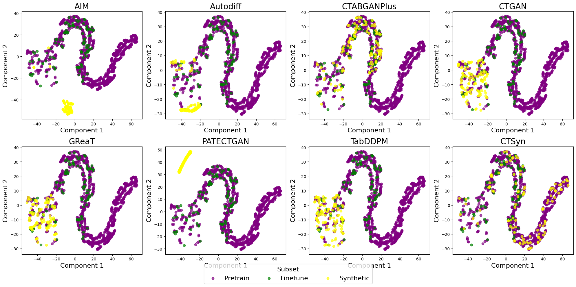
Figure 2: T-sne plot of obesity dataset from different synthesizers.

4.5 Ablation Study

We examine the significance of pre-training and task-specific decoders in the fine-tune setting of CTSyn. For effect of pre-training, we alternatively train the diffusion model and type-specific decoders only on fine-tune sets. For task-specific decoders, we replace type-specific decoders with an MLP decoder that reconstructs feature vectors and is trained solely on the fine-tune set. We present the utility and diversity results for each altered setting in Table 5 for the Synthesizing Diabetes dataset. Both alternative settings resulted in lower utility. Replacing the pre-trained decoders with data-specific decoders significantly increases data copying with lower PCT and DCR values. These findings indicate that pre-training enhances data diversity and mitigates the overfitting risk associated with data-specific decoding.

Table 5: Effect of model components on Diabete fine-tune set A.

Pre-train Diffusion	Decoder	Pre-train Decoder	Acc	F1	PCT	DCR
$\checkmark$	Type-specific	$\checkmark$	0.63	0.61	0.84	12.69
$\times$	Type-specific	$\checkmark$	0.60	0.58	0.80	2.80
$\checkmark$	Type-specific	$\times$	0.64	0.57	0.79	8.10
$\checkmark$	MLP	$\times$	0.61	0.57	0.36	4.15

5 Conclusion

In this paper, we introduced CTSyn, a pioneering framework within the realm of Generative Foundation Models (GFMs) for tabular data. Through extensive experimentation with real data, we demonstrated that CTSyn effectively leverages knowledge from diverse pre-trained tables to enhance synthetic data utility across various downstream datasets. To the best of our knowledge, our method is the first to consistently demonstrate a utility boost over real training data in downstream tasks, thereby paving the way for overcoming significant challenges in tabular data augmentation using deep generative models.

Appendix A Broader Impact

A foundational table generator like CTSyn can significantly enhance various application domains, especially where real data is scarce, sensitive, or expensive to obtain, by providing high-quality synthetic tabular data. In healthcare, for example, CTSyn can generate synthetic patient records that maintain statistical fidelity to real data, enhancing the robustness and generalization ability of machine learning models by augmenting datasets with synthetic data.

CTSyn also facilitates data collaboration between parties, such as advertising companies and social media websites. Through conditional generation, CTSyn can augment one party’s dataset with essential columns for business analysis without violating privacy laws that prohibit linking individual data points across parties.

However, CTSyn’s performance relies heavily on clean, large-scale tabular datasets. The quality of generated data depends on the training data, and any biases or errors can be propagated. This risk can be mitigated by carefully curating high-quality datasets for different domains. Additionally, despite pre-training reducing memorization of downstream data, individuals included in the pre-training data still face privacy risks, complicating the safe gathering of large datasets. This can be mitigated by properly anonymizing or adding noise to public pre-training datasets to ensure privacy before they are used for pre-training.

Appendix B Network Structures and Training

Number Auto-Encoder:

We use an auto-encoder to learn a latent space for quantiles uniformly distributed on Uniform(0,1). The encoder-decoder AE structure can be formally described as:

$$h_{0}=ReLU(FC_{1\to 1024}(x))$$

$$h_{1}=Tanh(FC_{1024\to 768}(h_{0}))\cdot 10$$

For the decoder:

$$d_{0}=ReLU(FC_{768\to 1024}(h_{1}))$$

$$d_{1}=FC_{1024\to 1}(d_{0})$$

For each epoch in pre-training, we sample $B=1024$ numbers from $\text{Uniform}(0,1)$, which match the range of transformed quantiles of numerical columns. Then the model is trained to reconstruct the input numbers with Mean-Squared Error(MSE) loss. Once pre-trained, the encoder part is used for projecting quantile-normalized values in all tables and tasks, to ensure consistency of embedding.

Aggregator and Decoders

For aggregator and decoders, we apply a Perceive Resampler [68] that learns latent vector $\bm{v}\in\mathbb{R}^{d_{\text{agg}}}$ that iteratively cross-attend to embeddings of the row features $E\in\mathbb{R}^{(2D+1)\times d_{\text{LM}}}$. Applying the same formulation as in [69], the learnable latent attend to both themselves and the input representation in each attention layer:

$$\bm{v}=\bm{v}+\text{MHA}(q=\bm{v},\text{kv}=[\bm{v};\bm{E}])$$

where $\text{MHA}(\cdot)$ is the multi-head attention operation with queries $q$ and keys/values kv. After each multi-head attention layer, a feedforward layer is applied to the latent representations.

For decoders, we apply one fully connected linear layer to downsize LM encoding of table metadata to the same dimension as $M_{\text{agg}}$. For numerical decoder, we apply one linear layer to map last layer representation to a 1 dimensional real number.

Both aggregator and decoders used a training batch size of 128, learning rate = $0.0005$, a cosine annealing schedule for learning rate and 1200 training epochs.

ResNet MLP

To model the reverse diffusion process, we use a Residual MLP architecture:

$$\text{ResMLPDiffusion}(x,t,y,\text{uncon\_rate})=\text{OutputLinear}(\text{ResMLPBlock}(\ldots(\text{ResMLPBlock}(x))))$$

Each ResMLPBlock consists of:

$$\text{ResMLPBlock}(x,t,y)=\text{SiLU}(\text{ResidualBlock}(x)$$

$$+\text{LinearBlock}(\text{TimestepEmbedding}(t))$$

$$+\text{LinearBlock}(y))$$

For the input, timestep, and conditional vector embeddings:

$$x=\text{SiLU}(\text{InputLinear}(x_{\text{in}}))$$

$$t_{\text{emb}}=\text{Linear}(\text{SiLU}(\text{Linear}(\text{SinTimeEmb}(t))))$$

$$y_{\text{emb}}=\text{SiLU}(\text{YLinear}(y))$$

The training setup includes both pre-training and fine-tuning phases. We use a batch size of 512 and 2500 timesteps. The Adam optimizer is employed with an initial learning rate of $5\times 10^{-4}$. The pre-training phase consists of 50000 epochs, while the fine-tuning phase is conducted for 10000 epochs.

Appendix C Baselines Implementation

CTGAN: We use the official implementation at https://github.com/sdv-dev/CTGAN. We use embedding dimension =128, generator dimension=(256,256), discriminator dimension =(256,256), generator learning rate=0.0002, generator decay =0.000001, discriminator learning rate =0.0002, discriminator decay =0.000001, batch size=500, training epoch = 300, discriminator steps=1, pac size = 5.

CTGAN-Plus: We used the official implementation at: https://github.com/Team-TUD/CTAB-GAN-Plus. We used default parameters: class dimensions =(256, 256, 256, 256), random dimensions=100, 64 channels, l2scale=1e-5, batch size=500, training epoch = 150.

Autodiff: We use the official implementation at https://github.com/UCLA-Trustworthy-AI-Lab/AutoDiffusion with default hyperparameters.

TabDDPM: We used the official implementation at https://github.com/yandex-research/tab-ddpm. We used 2500 diffusion steps, 10000 training epochs, learning rate = 0.001, weight decay = 1e-05, batch size = 1024.

AIM: We use the code implementation at https://github.com/ryan112358/private-pgm, with default parameters: epsilon=3,delta=1e-9,max model size=80

PATE-CTGAN: We adapted the implementation posted at: https://github.com/opendp/smartnoise-sdk/blob/main/synth/snsynth, which combines the PATE [59] learning framework with CTGAN. We use epsilon = 3, 5 iterations for student and teacher network, and the same value for other parameters which are shared with CTGAN.

GReaT: We used the official implementation at https://github.com/kathrinse/be_great/tree/main. We used a batch size of 64 and save steps of 400000. We following the pre-training pipeline outlined in [61]. During pre-training, we began with a randomized distilgpt2 model. For each pre-training dataset, we iteratively loaded the latest model, fitted the model on the new dataset, and saved the model to be used for the next iteration. We used 50 epochs for the health model and 200 epochs for the out-of-domain model. For finetuning, we fitted the pre-trained model on only one dataset using 200 epochs. The dataset used in finetuning was the dataset we wished to emulate during synthesis. For reference, we also fitted a newly randomized model on the data alone to serve as a base metric. During generation, we synthesized the same number of samples as the finetune dataset.

Appendix D Datasets

The link to datasets used is shown below:

NPHA: https://archive.ics.uci.edu/dataset/936/national+poll+on+healthy+aging+(npha)

Obesity: https://www.kaggle.com/code/mpwolke/obesity-levels-life-style

Diabetes: https://archi ve.ics.uci.edu/dataset/34/diabetes

India Liver Patient : https://www.kaggle.com/datasets/uciml/indian-liver-patient-records?resource=download

Sick: https://www.openml.org/search?type=data&sort=runs&id=38&status=active

Appendix E Statistical Similarity Metrics

We compute additional statistical similarity metrics for marginal column distributions: Wasserstein distance for numerical columns and Jensen-Shannon divergence for categorical columns. The results are shown in table 6. We observed that CTSyn achieved lower ranking in these distance metrics compared with SoTA baselines such as TabDDPM, indicating closer distance to real column distributions.

Table 6: Average Wasserstein Distance and Jansen-Shannon Distance between columns of real and synthetic tables. Lower ranks indicate better similarity.

Model	NPHA		Obesity		Diabetes		Liver		Sick		Avg Rank
	WS	JS	WS	JS	WS	JS	WS	JS	WS	JS	WS	JS
Real	0.48 (0.07)	0.48 (0.07)	0.57 (0.04)	0.57 (0.04)	0.48 (0.03)	0.48 (0.03)	0.55 (0.06)	0.55 (0.06)	0.40 (0.05)	0.40 (0.05)	7.20	7.20
CTGAN	0.48 (0.07)	0.48 (0.07)	0.57 (0.04)	0.57 (0.04)	inf (nan)	inf (nan)	0.53 (0.08)	0.53 (0.08)	0.42 (0.07)	0.42 (0.07)	5.30	5.30
CTABGANPlus	0.47 (0.07)	0.47 (0.07)	0.53 (0.05)	0.53 (0.05)	0.49 (0.03)	0.49 (0.03)	0.54 (0.06)	0.54 (0.06)	0.40 (0.04)	0.40 (0.04)	8.40	8.40
Autodiff	0.51 (0.05)	0.51 (0.05)	0.55 (0.04)	0.55 (0.04)	0.52 (0.06)	0.52 (0.06)	0.57 (0.09)	0.57 (0.09)	0.46 (0.06)	0.46 (0.06)	4.80	4.80
TabDDPM	0.50 (0.06)	0.50 (0.06)	0.57 (0.04)	0.57 (0.04)	0.48 (0.04)	0.48 (0.04)	0.54 (0.06)	0.54 (0.06)	0.42 (0.07)	0.42 (0.07)	5.40	5.40
AIM	0.54 (0.06)	0.54 (0.06)	0.57 (0.04)	0.57 (0.04)	0.48 (0.05)	0.48 (0.05)	0.54 (0.08)	0.54 (0.08)	0.47 (0.07)	0.47 (0.07)	4.80	4.80
PATECTGAN	0.50 (0.06)	0.50 (0.06)	0.56 (0.03)	0.56 (0.03)	inf (nan)	inf (nan)	0.51 (0.08)	0.51 (0.08)	0.44 (0.04)	0.44 (0.04)	6.10	6.10
GReaT	0.44 (0.11)	0.44 (0.11)	0.55 (0.03)	0.55 (0.03)	0.48 (0.01)	0.48 (0.01)	0.53 (0.07)	0.53 (0.07)	0.74 (0.01)	0.74 (0.01)	8.00	8.00
GReaT (Finetuned)	0.48 (0.08)	0.48 (0.08)	0.56 (0.04)	0.56 (0.04)	0.46 (0.02)	0.46 (0.02)	0.51 (0.08)	0.51 (0.08)	0.75 (0.01)	0.75 (0.01)	7.80	7.80
CTSyn (Finetuned)	0.45 (0.07)	0.45 (0.07)	0.58 (0.05)	0.58 (0.05)	0.49 (0.04)	0.49 (0.04)	0.56 (0.11)	0.56 (0.11)	0.39 (0.06)	0.39 (0.06)	6.20	6.20
CTSyn (Cond Gen)	0.51 (0.06)	0.51 (0.06)	0.58 (0.04)	0.58 (0.04)	0.44 (0.04)	0.44 (0.06)	0.53 (0.09)	0.53 (0.09)	0.40 (0.06)	0.40 (0.06)	6.60	6.60
CTSyn (Cond Aug)	0.52 (0.03)	0.52 (0.02)	0.55 (0.04)	0.55 (0.02)	0.43 (0.02)	0.43 (0.03)	0.63 (0.02)	0.63 (0.02)	0.38 (0.03)	0.38 (0.02)	7.40	7.40

Appendix F Cross-Domain Dataset Results Performance

We further validates the effectiveness of our method by performin the same pre-training/fine-tuning pipeline tables across different domains. The datasets tested and their summary statistics are shown in table 7:

Table 7: Summary statistics of cross-domain datasets.

Dataset	Rows	Categorical	Numerical	Domain
Abalone	4177	1	8	Biology
Churn Modeling	10000	3	8	Finance
Shoppers	12330	8	10	Marketing

We report the machine learning utility in table 8. We notice that CTSyn still consistently improve synthetic data generation with conditional generation, even for regression tasks.

Table 8: Machine learning utility of non-healthcare datasets.

Model	Abalone	Churn	Shoppers	Avg Rank
	$\text{Adjusted}R^{2}(\uparrow)$	$F1(\uparrow)$	$F1(\uparrow)$
Real	0.18	0.76	0.72	3.3
	(0.05)	(0.05)	(0.08)
CTGAN	-0.33	0.69	0.66	10
	(0.59)	(0.02)	(0.02)
CTABGANPlus	-0.09	0.70	0.66	9
	(0.17)	(0.02)	(0.05)
Autodiff	-1.26	0.68	0.63	11.3
	(1.53)	(0.14)	(0.13)
TabDDPM	0.13	0.74	0.73	4.7
	(0.06)	(0.04)	(0.06)
AIM	-0.02	0.71	0.69	8
	(0.10)	(0.06)	(0.03)
PATECTGAN	-7.76	0.62	0.71	10.3
	(0.19)	(0.08)	(0.08)
GReaT	-0.28	0.72	0.71	7.7
	(0.13)	(0.05)	(0.04)
GReaT (Finetuned)	0.15	0.75	0.73	3.7
	(0.13)	(0.05)	(0.03)
CTSyn (Finetuned)	0.10	0.75	0.74	4
	(0.19)	(0.04)	(0.04)
CTSyn (Cond Gen)	0.24	0.74	0.75	3
	(0.19)	(0.04)	(0.03)
CTSyn (Cond Aug)	0.29	0.76	0.80	1
	(0.02)	(0.04)	(0.02)

Appendix G Conditional Generation As Classification

We further test the conditional generation ability of our model by incorporating latent embedding of a subset of row features in the conditions. For each sample $\bm{v_{i}}$, we now create the corresponding condition $y_{i}$ by concatenating the the table context embedding $e_{m}$ with feature subset embedding $\bm{v_{i}^{+}}=f(E_{i}^{+})$ and $\bm{v_{i}^{-}}=f(E_{i}^{-})$, where $E_{i}^{+}$ and $E_{i}^{-}$ are created by masking the embedding of target columns‘s value and feature columns value in $E_{i}$ with a fixed vector of -1. We train the model on the pooled pre-train dataset, and test on the holdout test sets. During inference, we perform conditional generation and use type-specific decoder to decode value of the target column from the generated latent vector. We treat such conditional generation as a classification task.

Table 9 compares the classification performance using regular classifiers vs using CTSyn to perform conditional generation. Our model achieved similar F1 score as state-of-the-art classifier across dataset. Note that while the baseline classifiers are trained in a data-specific manner, our model is pre-trained across datasets and perform all such classifications with the same model. This showcases the potential of generative foundation model in other tabular tasks such as prediction and imputation.

Table 9: Classification F1 score with conditional generation and regular classifer models.

Model	Obesity	Diabetes	Sick	Liver 4	NPHA
Decision Tree	0.92	0.72	0.99	0.65	0.38
Random Forest	0.93	0.75	0.98	0.62	0.36
XGBoost	0.95	0.77	0.98	0.64	0.39
CTSyn	0.86	0.82	0.90	0.59	0.42

Appendix H Computation Cost

The experiments are performed on a Amazon AWS EC2 g5.4xlarge instance with an A10G tensor core GPU, 24 GB GPU Memory, 64GB RAM. The pre-training time is 24.5 hours for aggregator and decoders and 4 hrs for conditional diffusion model. The average fine-tuning time of conditional diffusion model is 6 minutes.

NeurIPS Paper Checklist

1. Claims

2. Question: Do the main claims made in the abstract and introduction accurately reflect the paper’s contributions and scope?

3. Answer: [Yes]

4. Justification: Our abstract and introduction accurately summarize the main contribution of 662 our method.

5. Guidelines:

   • The answer NA means that the abstract and introduction do not include the claims made in the paper.

   • The abstract and/or introduction should clearly state the claims made, including the contributions made in the paper and important assumptions and limitations. A No or NA answer to this question will not be perceived well by the reviewers.

   • The claims made should match theoretical and experimental results, and reflect how much the results can be expected to generalize to other settings.

   • It is fine to include aspirational goals as motivation as long as it is clear that these goals are not attained by the paper.

6. Limitations

7. Question: Does the paper discuss the limitations of the work performed by the authors?

8. Answer: [Yes]

9. Justification: See appendix section A.

10. Guidelines:

    • The answer NA means that the paper has no limitation while the answer No means that the paper has limitations, but those are not discussed in the paper.

    • The authors are encouraged to create a separate "Limitations" section in their paper.

    • The paper should point out any strong assumptions and how robust the results are to violations of these assumptions (e.g., independence assumptions, noiseless settings, model well-specification, asymptotic approximations only holding locally). The authors should reflect on how these assumptions might be violated in practice and what the implications would be.

    • The authors should reflect on the scope of the claims made, e.g., if the approach was only tested on a few datasets or with a few runs. In general, empirical results often depend on implicit assumptions, which should be articulated.

    • The authors should reflect on the factors that influence the performance of the approach. For example, a facial recognition algorithm may perform poorly when image resolution is low or images are taken in low lighting. Or a speech-to-text system might not be used reliably to provide closed captions for online lectures because it fails to handle technical jargon.

    • The authors should discuss the computational efficiency of the proposed algorithms and how they scale with dataset size.

    • If applicable, the authors should discuss possible limitations of their approach to address problems of privacy and fairness.

    • While the authors might fear that complete honesty about limitations might be used by reviewers as grounds for rejection, a worse outcome might be that reviewers discover limitations that aren’t acknowledged in the paper. The authors should use their best judgment and recognize that individual actions in favor of transparency play an important role in developing norms that preserve the integrity of the community. Reviewers will be specifically instructed to not penalize honesty concerning limitations.

11. Theory Assumptions and Proofs

12. Question: For each theoretical result, does the paper provide the full set of assumptions and a complete (and correct) proof?

13. Answer: [N/A]

14. Justification: This paper does not include theoretical results.

15. Guidelines:

    • The answer NA means that the paper does not include theoretical results.

    • All the theorems, formulas, and proofs in the paper should be numbered and cross-referenced.

    • All assumptions should be clearly stated or referenced in the statement of any theorems.

    • The proofs can either appear in the main paper or the supplemental material, but if they appear in the supplemental material, the authors are encouraged to provide a short proof sketch to provide intuition.

    • Inversely, any informal proof provided in the core of the paper should be complemented by formal proofs provided in appendix or supplemental material.

    • Theorems and Lemmas that the proof relies upon should be properly referenced.

16. Experimental Result Reproducibility

17. Question: Does the paper fully disclose all the information needed to reproduce the main experimental results of the paper to the extent that it affects the main claims and/or conclusions of the paper (regardless of whether the code and data are provided or not)?

18. Answer: [Yes]

19. Justification: We have fully described implementation of our proposed method in section 3 and baselines methods in appendix section C. We have also included the fully code implementation of our method.

20. Guidelines:

    • The answer NA means that the paper does not include experiments.

    • If the paper includes experiments, a No answer to this question will not be perceived well by the reviewers: Making the paper reproducible is important, regardless of whether the code and data are provided or not.

    • If the contribution is a dataset and/or model, the authors should describe the steps taken to make their results reproducible or verifiable.

    • Depending on the contribution, reproducibility can be accomplished in various ways. For example, if the contribution is a novel architecture, describing the architecture fully might suffice, or if the contribution is a specific model and empirical evaluation, it may be necessary to either make it possible for others to replicate the model with the same dataset, or provide access to the model. In general. releasing code and data is often one good way to accomplish this, but reproducibility can also be provided via detailed instructions for how to replicate the results, access to a hosted model (e.g., in the case of a large language model), releasing of a model checkpoint, or other means that are appropriate to the research performed.

    • While NeurIPS does not require releasing code, the conference does require all submissions to provide some reasonable avenue for reproducibility, which may depend on the nature of the contribution. For example

      1. If the contribution is primarily a new algorithm, the paper should make it clear how to reproduce that algorithm.

      2. If the contribution is primarily a new model architecture, the paper should describe the architecture clearly and fully.

      3. If the contribution is a new model (e.g., a large language model), then there should either be a way to access this model for reproducing the results or a way to reproduce the model (e.g., with an open-source dataset or instructions for how to construct the dataset).

      4. We recognize that reproducibility may be tricky in some cases, in which case authors are welcome to describe the particular way they provide for reproducibility. In the case of closed-source models, it may be that access to the model is limited in some way (e.g., to registered users), but it should be possible for other researchers to have some path to reproducing or verifying the results.

21. Open access to data and code

22. Question: Does the paper provide open access to the data and code, with sufficient instructions to faithfully reproduce the main experimental results, as described in supplemental material?

23. Answer: [No]

24. Justification: The evaluation code of this paper uses proprietary repositories. Thus the full code to reproduce results will be made publicly available upon acceptance.

25. Guidelines:

    • The answer NA means that paper does not include experiments requiring code.

    • Please see the NeurIPS code and data submission guidelines (https://nips.cc/public/guides/CodeSubmissionPolicy) for more details.

    • While we encourage the release of code and data, we understand that this might not be possible, so “No” is an acceptable answer. Papers cannot be rejected simply for not including code, unless this is central to the contribution (e.g., for a new open-source benchmark).

    • The instructions should contain the exact command and environment needed to run to reproduce the results. See the NeurIPS code and data submission guidelines (https://nips.cc/public/guides/CodeSubmissionPolicy) for more details.

    • The authors should provide instructions on data access and preparation, including how to access the raw data, preprocessed data, intermediate data, and generated data, etc.

    • The authors should provide scripts to reproduce all experimental results for the new proposed method and baselines. If only a subset of experiments are reproducible, they should state which ones are omitted from the script and why.

    • At submission time, to preserve anonymity, the authors should release anonymized versions (if applicable).

    • Providing as much information as possible in supplemental material (appended to the paper) is recommended, but including URLs to data and code is permitted.

26. Experimental Setting/Details

27. Question: Does the paper specify all the training and test details (e.g., data splits, hyperparameters, how they were chosen, type of optimizer, etc.) necessary to understand the results?

28. Answer: [Yes]

29. Justification: We have fully described implementation of our proposed method and baselines being compared, including the network structure, training process and hyper-parameters used, in both main text and technical appendix.

30. Guidelines:

    • The answer NA means that the paper does not include experiments.

    • The experimental setting should be presented in the core of the paper to a level of detail that is necessary to appreciate the results and make sense of them.

    • The full details can be provided either with the code, in appendix, or as supplemental material.

31. Experiment Statistical Significance

32. Question: Does the paper report error bars suitably and correctly defined or other appropriate information about the statistical significance of the experiments?

33. Answer: [Yes]

34. Justification: For all experiment results, we repeated 10 trials with finetune/holdout test set splits created using random seeds 0 to 9. The standard deviation for scores across all trials are reported alongside the average scores.

35. Guidelines:

    • The answer NA means that the paper does not include experiments.

    • The authors should answer "Yes" if the results are accompanied by error bars, confidence intervals, or statistical significance tests, at least for the experiments that support the main claims of the paper.

    • The factors of variability that the error bars are capturing should be clearly stated (for example, train/test split, initialization, random drawing of some parameter, or overall run with given experimental conditions).

    • The method for calculating the error bars should be explained (closed form formula, call to a library function, bootstrap, etc.)

    • The assumptions made should be given (e.g., Normally distributed errors).

    • It should be clear whether the error bar is the standard deviation or the standard error of the mean.

    • It is OK to report 1-sigma error bars, but one should state it. The authors should preferably report a 2-sigma error bar than state that they have a 96% CI, if the hypothesis of Normality of errors is not verified.

    • For asymmetric distributions, the authors should be careful not to show in tables or figures symmetric error bars that would yield results that are out of range (e.g. negative error rates).

    • If error bars are reported in tables or plots, The authors should explain in the text how they were calculated and reference the corresponding figures or tables in the text.

36. Experiments Compute Resources

37. Question: For each experiment, does the paper provide sufficient information on the computer resources (type of compute workers, memory, time of execution) needed to reproduce the experiments?

38. Answer: [Yes]

39. Justification: In the appendix section H, we detailed the hardware used for computing as well as runtime under the training parameter specified in the main text

40. Guidelines:

    • The answer NA means that the paper does not include experiments.

    • The paper should indicate the type of compute workers CPU or GPU, internal cluster, or cloud provider, including relevant memory and storage.

    • The paper should provide the amount of compute required for each of the individual experimental runs as well as estimate the total compute.

    • The paper should disclose whether the full research project required more compute than the experiments reported in the paper (e.g., preliminary or failed experiments that didn’t make it into the paper).

41. Code Of Ethics

42. Question: Does the research conducted in the paper conform, in every respect, with the NeurIPS Code of Ethics https://neurips.cc/public/EthicsGuidelines?

43. Answer: [Yes]

44. Justification: We have reviewed the NeurIPS Code of Ethics and ensure our study aligns with it.

45. Guidelines:

    • The answer NA means that the authors have not reviewed the NeurIPS Code of Ethics.

    • If the authors answer No, they should explain the special circumstances that require a deviation from the Code of Ethics.

    • The authors should make sure to preserve anonymity (e.g., if there is a special consideration due to laws or regulations in their jurisdiction).

46. Broader Impacts

47. Question: Does the paper discuss both potential positive societal impacts and negative societal impacts of the work performed?

48. Answer: [Yes]

49. Justification: Please see appendix section A.

50. Guidelines:

    • The answer NA means that there is no societal impact of the work performed.

    • If the authors answer NA or No, they should explain why their work has no societal impact or why the paper does not address societal impact.

    • Examples of negative societal impacts include potential malicious or unintended uses (e.g., disinformation, generating fake profiles, surveillance), fairness considerations (e.g., deployment of technologies that could make decisions that unfairly impact specific groups), privacy considerations, and security considerations.

    • The conference expects that many papers will be foundational research and not tied to particular applications, let alone deployments. However, if there is a direct path to any negative applications, the authors should point it out. For example, it is legitimate to point out that an improvement in the quality of generative models could be used to generate deepfakes for disinformation. On the other hand, it is not needed to point out that a generic algorithm for optimizing neural networks could enable people to train models that generate Deepfakes faster.

    • The authors should consider possible harms that could arise when the technology is being used as intended and functioning correctly, harms that could arise when the technology is being used as intended but gives incorrect results, and harms following from (intentional or unintentional) misuse of the technology.

    • If there are negative societal impacts, the authors could also discuss possible mitigation strategies (e.g., gated release of models, providing defenses in addition to attacks, mechanisms for monitoring misuse, mechanisms to monitor how a system learns from feedback over time, improving the efficiency and accessibility of ML).

51. Safeguards

52. Question: Does the paper describe safeguards that have been put in place for responsible release of data or models that have a high risk for misuse (e.g., pretrained language models, image generators, or scraped datasets)?

53. Answer: [N/A]

54. Justification: This paper does not release any pre-trained model or scrapped dataset. The algorithm we describe and results presented are trained on public datasets.

55. Guidelines:

    • The answer NA means that the paper poses no such risks.

    • Released models that have a high risk for misuse or dual-use should be released with necessary safeguards to allow for controlled use of the model, for example by requiring that users adhere to usage guidelines or restrictions to access the model or implementing safety filters.

    • Datasets that have been scraped from the Internet could pose safety risks. The authors should describe how they avoided releasing unsafe images.

    • We recognize that providing effective safeguards is challenging, and many papers do not require this, but we encourage authors to take this into account and make a best faith effort.

56. Licenses for existing assets

57. Question: Are the creators or original owners of assets (e.g., code, data, models), used in the paper, properly credited and are the license and terms of use explicitly mentioned and properly respected?

58. Answer: [Yes]

59. Justification: We have added proper references and/or link to all datasets, code implementa tion of baseline methods, model architecture used and/or adapted, and pre-trained models used in this paper.

60. Guidelines:

    • The answer NA means that the paper does not use existing assets.

    • The authors should cite the original paper that produced the code package or dataset.

    • The authors should state which version of the asset is used and, if possible, include a URL.

    • The name of the license (e.g., CC-BY 4.0) should be included for each asset.

    • For scraped data from a particular source (e.g., website), the copyright and terms of service of that source should be provided.

    • If assets are released, the license, copyright information, and terms of use in the package should be provided. For popular datasets, paperswithcode.com/datasets has curated licenses for some datasets. Their licensing guide can help determine the license of a dataset.

    • For existing datasets that are re-packaged, both the original license and the license of the derived asset (if it has changed) should be provided.

    • If this information is not available online, the authors are encouraged to reach out to the asset’s creators.

61. New Assets

62. Question: Are new assets introduced in the paper well documented and is the documentation provided alongside the assets?

63. Answer: [Yes]

64. Justification: The code implementation of the proposed algorithm, developed solely by the authors, is included in the supplementary material. The structural and implementation details are fully described in the main text and appendix, providing comprehensive documentation alongside the assets.

65. Guidelines:

    • The answer NA means that the paper does not release new assets.

    • Researchers should communicate the details of the dataset/code/model as part of their submissions via structured templates. This includes details about training, license, limitations, etc.

    • The paper should discuss whether and how consent was obtained from people whose asset is used.

    • At submission time, remember to anonymize your assets (if applicable). You can either create an anonymized URL or include an anonymized zip file.

66. Crowdsourcing and Research with Human Subjects

67. Question: For crowdsourcing experiments and research with human subjects, does the paper include the full text of instructions given to participants and screenshots, if applicable, as well as details about compensation (if any)?

68. Answer: [N/A]

69. Justification: This paper does not involve crowdsourcing nor research with human subjects.

70. Guidelines:

    • The answer NA means that the paper does not involve crowdsourcing nor research with human subjects.

    • Including this information in the supplemental material is fine, but if the main contribution of the paper involves human subjects, then as much detail as possible should be included in the main paper.

    • According to the NeurIPS Code of Ethics, workers involved in data collection, curation, or other labor should be paid at least the minimum wage in the country of the data collector.

71. Institutional Review Board (IRB) Approvals or Equivalent for Research with Human Subjects

72. Question: Does the paper describe potential risks incurred by study participants, whether such risks were disclosed to the subjects, and whether Institutional Review Board (IRB) approvals (or an equivalent approval/review based on the requirements of your country or institution) were obtained?

73. Answer: [N/A]

74. Justification: This paper does not involve crowdsourcing nor research with human subjects.

75. Guidelines:

    • The answer NA means that the paper does not involve crowdsourcing nor research with human subjects.

    • Depending on the country in which research is conducted, IRB approval (or equivalent) may be required for any human subjects research. If you obtained IRB approval, you should clearly state this in the paper.

    • We recognize that the procedures for this may vary significantly between institutions and locations, and we expect authors to adhere to the NeurIPS Code of Ethics and the guidelines for their institution.

    • For initial submissions, do not include any information that would break anonymity (if applicable), such as the institution conducting the review.

References

- [1] Rishi Bommasani, Drew A Hudson, Ehsan Adeli, Russ Altman, Simran Arora, Sydney von Arx, Michael S Bernstein, Jeannette Bohg, Antoine Bosselut, Emma Brunskill, et al. On the opportunities and risks of foundation models. arXiv preprint arXiv:2108.07258, 2021.
- [2] Kaiming He, Xiangyu Zhang, Shaoqing Ren, and Jian Sun. Deep residual learning for image recognition. In Proceedings of the IEEE conference on computer vision and pattern recognition, pages 770–778, 2016.
- [3] OpenAI. Gpt-4 technical report. arXiv preprint arXiv:2303.08774, 2023.
- [4] Hugo Touvron, Louis Martin, Kevin Stone, Peter Albert, Amjad Almahairi, Yasmine Babaei, Nikolay Bashlykov, Soumya Batra, Prajjwal Bhargava, Shruti Bhosale, et al. Llama 2: Open foundation and fine-tuned chat models. arXiv preprint arXiv:2307.09288, 2023.
- [5] Aditya Ramesh, Prafulla Dhariwal, Alex Nichol, Casey Chu, and Mark Chen. Hierarchical text-conditional image generation with clip latents. arXiv preprint arXiv:2204.06125, 2022.
- [6] Robin Rombach, Andreas Blattmann, Dominik Lorenz, Patrick Esser, and Björn Ommer. High-resolution image synthesis with latent diffusion models. In Proceedings of the IEEE/CVF conference on computer vision and pattern recognition, pages 10684–10695, 2022.
- [7] Stephen Merity, Caiming Xiong, James Bradbury, and Richard Socher. Pointer sentinel mixture models. arXiv preprint arXiv:1609.07843, 2016.
- [8] Jia Deng, Wei Dong, Richard Socher, Li-Jia Li, Kai Li, and Li Fei-Fei. Imagenet: A large-scale hierarchical image database. In 2009 IEEE conference on computer vision and pattern recognition, pages 248–255. Ieee, 2009.
- [9] Christoph Schuhmann, Romain Beaumont, Richard Vencu, Cade Gordon, Ross Wightman, Mehdi Cherti, Theo Coombes, Aarush Katta, Clayton Mullis, Mitchell Wortsman, et al. Laion-5b: An open large-scale dataset for training next generation image-text models. Advances in Neural Information Processing Systems, 35:25278–25294, 2022.
- [10] Ashish Vaswani, Noam Shazeer, Niki Parmar, Jakob Uszkoreit, Llion Jones, Aidan N Gomez, Łukasz Kaiser, and Illia Polosukhin. Attention is all you need. Advances in neural information processing systems, 30, 2017.
- [11] Jonathan Ho, Ajay Jain, and Pieter Abbeel. Denoising diffusion probabilistic models. Advances in neural information processing systems, 33:6840–6851, 2020.
- [12] Alexander Kirillov, Eric Mintun, Nikhila Ravi, Hanzi Mao, Chloe Rolland, Laura Gustafson, Tete Xiao, Spencer Whitehead, Alexander C Berg, Wan-Yen Lo, et al. Segment anything. arXiv preprint arXiv:2304.02643, 2023.
- [13] Zhuoyan Li, Hangxiao Zhu, Zhuoran Lu, and Ming Yin. Synthetic data generation with large language models for text classification: Potential and limitations. In The 2023 Conference on Empirical Methods in Natural Language Processing, 2023.
- [14] Michael Moor, Oishi Banerjee, Zahra Shakeri Hossein Abad, Harlan M Krumholz, Jure Leskovec, Eric J Topol, and Pranav Rajpurkar. Foundation models for generalist medical artificial intelligence. Nature, 616(7956):259–265, 2023.
- [15] Brandon Trabucco, Kyle Doherty, Max A Gurinas, and Ruslan Salakhutdinov. Effective data augmentation with diffusion models. In The Twelfth International Conference on Learning Representations, 2023.
- [16] Boyu Zhang, Hongyang Yang, Tianyu Zhou, Muhammad Ali Babar, and Xiao-Yang Liu. Enhancing financial sentiment analysis via retrieval augmented large language models. In Proceedings of the Fourth ACM International Conference on AI in Finance, pages 349–356, 2023.
- [17] Sabyasachi Dash, Sushil Kumar Shakyawar, Mohit Sharma, and Sandeep Kaushik. Big data in healthcare: management, analysis and future prospects. Journal of big data, 6(1):1–25, 2019.
- [18] Vadim Borisov, Tobias Leemann, Kathrin Seßler, Johannes Haug, Martin Pawelczyk, and Gjergji Kasneci. Deep neural networks and tabular data: A survey. IEEE Transactions on Neural Networks and Learning Systems, 2022.
- [19] Ravid Shwartz-Ziv and Amitai Armon. Tabular data: Deep learning is not all you need. Information Fusion, 81:84–90, 2022.
- [20] Lei Xu, Maria Skoularidou, Alfredo Cuesta-Infante, and Kalyan Veeramachaneni. Modeling tabular data using conditional gan. Advances in neural information processing systems, 32, 2019.
- [21] Akim Kotelnikov, Dmitry Baranchuk, Ivan Rubachev, and Artem Babenko. Tabddpm: Modelling tabular data with diffusion models. In International Conference on Machine Learning, pages 17564–17579. PMLR, 2023.
- [22] Ryan McKenna, Brett Mullins, Daniel Sheldon, and Gerome Miklau. Aim: an adaptive and iterative mechanism for differentially private synthetic data. Proceedings of the VLDB Endowment, 15(11):2599–2612, 2022.
- [23] Yotam Elor and Hadar Averbuch-Elor. To smote, or not to smote? arXiv preprint arXiv:2201.08528, 2022.
- [24] Dionysis Manousakas and Sergül Aydöre. On the usefulness of synthetic tabular data generation. arXiv preprint arXiv:2306.15636, 2023.
- [25] Soma Onishi, Kenta Oono, and Kohei Hayashi. Tabret: Pre-training transformer-based tabular models for unseen columns. In ICLR 2023 Workshop on Mathematical and Empirical Understanding of Foundation Models, 2023.
- [26] Xin Huang, Ashish Khetan, Milan Cvitkovic, and Zohar Karnin. Tabtransformer: Tabular data modeling using contextual embeddings. arXiv preprint arXiv:2012.06678, 2020.
- [27] Bingzhao Zhu, Xingjian Shi, Nick Erickson, Mu Li, George Karypis, and Mahsa Shoaran. Xtab: cross-table pretraining for tabular transformers. In Proceedings of the 40th International Conference on Machine Learning, pages 43181–43204, 2023.
- [28] Chao Ye, Guoshan Lu, Haobo Wang, Liyao Li, Sai Wu, Gang Chen, and Junbo Zhao. Ct-bert: Learning better tabular representations through cross-table pre-training. arXiv preprint arXiv:2307.04308, 2023.
- [29] Boris van Breugel and Mihaela van der Schaar. Why tabular foundation models should be a research priority. arXiv preprint arXiv:2405.01147, 2024.
- [30] Zifeng Wang and Jimeng Sun. Transtab: Learning transferable tabular transformers across tables. Advances in Neural Information Processing Systems, 35:2902–2915, 2022.
- [31] Stefan Hegselmann, Alejandro Buendia, Hunter Lang, Monica Agrawal, Xiaoyi Jiang, and David Sontag. Tabllm: Few-shot classification of tabular data with large language models. In International Conference on Artificial Intelligence and Statistics, pages 5549–5581. PMLR, 2023.
- [32] Jiahuan Yan, Bo Zheng, Hongxia Xu, Yiheng Zhu, Danny Chen, Jimeng Sun, Jian Wu, and Jintai Chen. Making pre-trained language models great on tabular prediction. In The Twelfth International Conference on Learning Representations, 2024.
- [33] Han-Jia Ye, Qile Zhou, and De-Chuan Zhan. Training-free generalization on heterogeneous tabular data via meta-representation. 2023.
- [34] Suchin Gururangan, Ana Marasović, Swabha Swayamdipta, Kyle Lo, Iz Beltagy, Doug Downey, and Noah A Smith. Don’t stop pretraining: Adapt language models to domains and tasks. In Proceedings of the 58th Annual Meeting of the Association for Computational Linguistics, pages 8342–8360, 2020.
- [35] Xin Yuan, Zhe Lin, Jason Kuen, Jianming Zhang, Yilin Wang, Michael Maire, Ajinkya Kale, and Baldo Faieta. Multimodal contrastive training for visual representation learning. In Proceedings of the IEEE/CVF Conference on Computer Vision and Pattern Recognition (CVPR), pages 6995–7004, June 2021.
- [36] Colin Wei, Sang Michael Xie, and Tengyu Ma. Why do pretrained language models help in downstream tasks? an analysis of head and prompt tuning. Advances in Neural Information Processing Systems, 34:16158–16170, 2021.
- [37] Xiaokang Chen, Mingyu Ding, Xiaodi Wang, Ying Xin, Shentong Mo, Yunhao Wang, Shumin Han, Ping Luo, Gang Zeng, and Jingdong Wang. Context autoencoder for self-supervised representation learning. International Journal of Computer Vision, 132(1):208–223, 2024.
- [38] Jinsung Yoon, Yao Zhang, James Jordon, and Mihaela Van der Schaar. Vime: Extending the success of self-and semi-supervised learning to tabular domain. Advances in Neural Information Processing Systems, 33:11033–11043, 2020.
- [39] Dara Bahri, Heinrich Jiang, Yi Tay, and Donald Metzler. Scarf: Self-supervised contrastive learning using random feature corruption. In International Conference on Learning Representations, 2022.
- [40] Talip Ucar, Ehsan Hajiramezanali, and Lindsay Edwards. Subtab: Subsetting features of tabular data for self-supervised representation learning. Advances in Neural Information Processing Systems, 34:18853–18865, 2021.
- [41] Sharad Chitlangia, Anand Muralidhar, and Rajat Agarwal. Self supervised pre-training for large scale tabular data. 2022.
- [42] Scott Yak, Yihe Dong, Javier Gonzalvo, and Sercan Arik. Ingestables: Scalable and efficient training of llm-enabled tabular foundation models. In NeurIPS 2023 Second Table Representation Learning Workshop, 2023.
- [43] Yazheng Yang, Yuqi Wang, Guang Liu, Ledell Wu, and Qi Liu. Unitabe: A universal pretraining protocol for tabular foundation model in data science. In The Twelfth International Conference on Learning Representations, 2024.
- [44] Tuan Dinh, Yuchen Zeng, Ruisu Zhang, Ziqian Lin, Michael Gira, Shashank Rajput, Jy-yong Sohn, Dimitris Papailiopoulos, and Kangwook Lee. Lift: Language-interfaced fine-tuning for non-language machine learning tasks. Advances in Neural Information Processing Systems, 35:11763–11784, 2022.
- [45] Vadim Borisov, Kathrin Sessler, Tobias Leemann, Martin Pawelczyk, and Gjergji Kasneci. Language models are realistic tabular data generators. In The Eleventh International Conference on Learning Representations, 2023.
- [46] Guang Liu, Jie Yang, and Ledell Wu. Ptab: Using the pre-trained language model for modeling tabular data. arXiv preprint arXiv:2209.08060, 2022.
- [47] Tianping Zhang, Shaowen Wang, YAN Shuicheng, Li Jian, and Qian Liu. Generative table pre-training empowers models for tabular prediction. In The 2023 Conference on Empirical Methods in Natural Language Processing, 2023.
- [48] Han Zhang, Xumeng Wen, Shun Zheng, Wei Xu, and Jiang Bian. Towards foundation models for learning on tabular data. arXiv preprint arXiv:2310.07338, 2023.
- [49] Beata Nowok, Gillian M Raab, and Chris Dibben. synthpop: Bespoke creation of synthetic data in r. Journal of statistical software, 74:1–26, 2016.
- [50] Jerome P Reiter. Using cart to generate partially synthetic public use microdata. Journal of official statistics, 21(3):441, 2005.
- [51] Nitesh V Chawla, Kevin W Bowyer, Lawrence O Hall, and W Philip Kegelmeyer. Smote: synthetic minority over-sampling technique. Journal of artificial intelligence research, 16:321–357, 2002.
- [52] Zhengping Che, Yu Cheng, Shuangfei Zhai, Zhaonan Sun, and Yan Liu. Boosting deep learning risk prediction with generative adversarial networks for electronic health records. In 2017 IEEE International Conference on Data Mining (ICDM), pages 787–792. IEEE, 2017.
- [53] Jayoung Kim, Jinsung Jeon, Jaehoon Lee, Jihyeon Hyeong, and Noseong Park. Oct-gan: Neural ode-based conditional tabular gans. In Proceedings of the Web Conference 2021, pages 1506–1515, 2021.
- [54] Alvaro Figueira and Bruno Vaz. Survey on synthetic data generation, evaluation methods and gans. Mathematics, 10(15):2733, 2022.
- [55] Zilong Zhao, Aditya Kunar, Robert Birke, and Lydia Y Chen. Ctab-gan: Effective table data synthesizing. In Asian Conference on Machine Learning, pages 97–112. PMLR, 2021.
- [56] Zilong Zhao, Aditya Kunar, Robert Birke, Hiek Van der Scheer, and Lydia Y Chen. Ctab-gan+: Enhancing tabular data synthesis. Frontiers in big Data, 6:1296508, 2024.
- [57] Namjoon Suh, Xiaofeng Lin, Din-Yin Hsieh, Merhdad Honarkhah, and Guang Cheng. Autodiff: combining auto-encoder and diffusion model for tabular data synthesizing. CoRR, abs/2310.15479, 2023.
- [58] Hengrui Zhang, Jiani Zhang, Zhengyuan Shen, Balasubramaniam Srinivasan, Xiao Qin, Christos Faloutsos, Huzefa Rangwala, and George Karypis. Mixed-type tabular data synthesis with score-based diffusion in latent space. In The Twelfth International Conference on Learning Representations, 2024.
- [59] James Jordon, Jinsung Yoon, and Mihaela Van Der Schaar. Pate-gan: Generating synthetic data with differential privacy guarantees. In International conference on learning representations, 2018.
- [60] Jun Zhang, Graham Cormode, Cecilia M Procopiuc, Divesh Srivastava, and Xiaokui Xiao. Privbayes: Private data release via bayesian networks. ACM Transactions on Database Systems (TODS), 42(4):1–41, 2017.
- [61] Zilong Zhao, Robert Birke, and Lydia Chen. Tabula: Harnessing language models for tabular data synthesis. arXiv preprint arXiv:2310.12746, 2023.
- [62] Eric Wallace, Yizhong Wang, Sujian Li, Sameer Singh, and Matt Gardner. Do nlp models know numbers? probing numeracy in embeddings. In Proceedings of the 2019 Conference on Empirical Methods in Natural Language Processing and the 9th International Joint Conference on Natural Language Processing (EMNLP-IJCNLP), pages 5307–5315, 2019.
- [63] F. Pedregosa, G. Varoquaux, A. Gramfort, V. Michel, B. Thirion, O. Grisel, M. Blondel, P. Prettenhofer, R. Weiss, V. Dubourg, J. Vanderplas, A. Passos, D. Cournapeau, M. Brucher, M. Perrot, and E. Duchesnay. Scikit-learn: Machine learning in Python. Journal of Machine Learning Research, 12:2825–2830, 2011.
- [64] Alec Radford, Jong Wook Kim, Chris Hallacy, Aditya Ramesh, Gabriel Goh, Sandhini Agarwal, Girish Sastry, Amanda Askell, Pamela Mishkin, Jack Clark, et al. Learning transferable visual models from natural language supervision. In International conference on machine learning, pages 8748–8763. PMLR, 2021.
- [65] Ian Goodfellow, Yoshua Bengio, and Aaron Courville. Deep Learning. MIT Press, 2016. http://www.deeplearningbook.org.
- [66] Tianhe Yu, Saurabh Kumar, Abhishek Gupta, Sergey Levine, Karol Hausman, and Chelsea Finn. Gradient surgery for multi-task learning. Advances in Neural Information Processing Systems, 33:5824–5836, 2020.
- [67] Zehan Li, Xin Zhang, Yanzhao Zhang, Dingkun Long, Pengjun Xie, and Meishan Zhang. Towards general text embeddings with multi-stage contrastive learning. arXiv preprint arXiv:2308.03281, 2023.
- [68] Lu Yuan, Dongdong Chen, Yi-Ling Chen, Noel Codella, Xiyang Dai, Jianfeng Gao, Houdong Hu, Xuedong Huang, Boxin Li, Chunyuan Li, et al. Florence: A new foundation model for computer vision. arXiv preprint arXiv:2111.11432, 2021.
- [69] Justin Lovelace, Varsha Kishore, Chao Wan, Eliot Shekhtman, and Kilian Q Weinberger. Latent diffusion for language generation. Advances in Neural Information Processing Systems, 36, 2024.
- [70] Tianqi Chen and Carlos Guestrin. Xgboost: A scalable tree boosting system. In Proceedings of the 22nd acm sigkdd international conference on knowledge discovery and data mining, pages 785–794, 2016.
- [71] Liudmila Prokhorenkova, Gleb Gusev, Aleksandr Vorobev, Anna Veronika Dorogush, and Andrey Gulin. Catboost: unbiased boosting with categorical features. Advances in neural information processing systems, 31, 2018.
- [72] Michael Platzer and Thomas Reutterer. Holdout-based empirical assessment of mixed-type synthetic data. Frontiers in big Data, 4:679939, 2021.