JWST view of three infant galaxies at $z=8.3$ and implications for reionization

Abstract

New JWST/NIRCam wide-field slitless spectroscopy provides redshifts for two $z>8$ galaxies located behind the lensing cluster MACS J0416.1$-$2403. Both galaxies are strong [O 3] $\lambda$5007 emitters. For one galaxy, “Y1,” the existing redshift $z=8.31$, based on ALMA measurements of [O 3] 88 $\mu$m and [C 2] 157.7 $\mu$m lines, is confirmed. JWST/NIRCam images resolve this galaxy into three components of similar colors, and the whole system extends over $\sim$3.4 kpc. The other galaxy, “JD,” is at $z=8.34$ instead of the previously claimed $z=9.28$. It has a companion, “JD-N,” at the same redshift with projected separation $\sim$2.3 kpc. All objects are only moderately magnified and have intrinsic $M_{\rm UV}$ ranging from $-19.66$ to $-20.85$ mag. Their eight-band NIRCam spectral energy distributions show that the galaxies are all very young with ages $\lesssim$11 Myr and stellar masses about $10^{8}$ ${\rm M_{\odot}}$. These infant galaxies are actively forming stars at rates of a few tens to a couple of hundred $\rm{M_{\odot}}$ yr^-1, but only one of them (JD) has a blue rest-frame UV slope. This slope indicates a high Lyman-continuum photon escape fraction that could contribute significantly to the cosmic hydrogen-reionizing background. The other two systems have much flatter slopes largely because their dust extinction is twice as high as JD’s albeit only $A_{V}\sim 0.90$ mag. The much lower indicated escape fractions show that even very young, actively star-forming galaxies can have negligible contribution to reionization when they quickly form dust throughout their bodies.

1 Introduction

Young, star-forming galaxies are long thought to be the major drivers of the cosmic hydrogen reionization because they should have strong UV emission and are sufficiently abundant at $z>6$ (e.g., Yan & Windhorst, 2004; Bouwens et al., 2006; Finkelstein et al., 2012; Robertson, 2022). Their exact contribution to the ionizing photon background, however, still depends on how effectively their Lyman continuum (LyC; $\lambda<912$Å) photons can escape and reach the surrounding intergalactic medium (IGM). Direct measurement of this escape fraction ($f_{\rm esc}$) for star-forming galaxies at $z>6$ is impossible, because the line-of-sight IGM H 1 absorption at such redshifts wipes out any LyC photons. As the alternative, $f_{\rm esc}$ has been measured for the “analogs” at lower redshifts ($z\lesssim 3$–4) where the IGM hydrogen is fully ionized (e.g. Steidel et al., 2001, 2018; Vanzella et al., 2012; Siana et al., 2015; Grazian et al., 2016; Izotov et al., 2016, 2018, 2021; Saldana-Lopez et al., 2022; Griffiths et al., 2022; Flury et al., 2022), and the correlations between $f_{\rm esc}$ and various observables are sought after in order to provide some viable routes to indirectly measure $f_{\rm esc}$ at $z>6$. Among all possible correlations, the one with the rest-frame UV slope (commonly denoted as $\beta$; $f_{\lambda}\propto\lambda^{\beta}$) is the most promising (e.g., Zackrisson et al., 2013; Chisholm et al., 2022).

There have been ample studies of the UV slopes of galaxies at $z>6$ using the Hubble Space Telescope (HST) deep survey data (e.g., Hathi et al., 2008; Bouwens et al., 2010; Dunlop et al., 2012, 2013; Finkelstein et al., 2012), and the investigation has been extended to higher redshifts and fainter limits by the James Webb Space Telescope (JWST; e.g., Topping et al., 2022; Cullen et al., 2023; Nanayakkara et al., 2023; Morales et al., 2024; Austin et al., 2024). However, the vast majority of those are based on photometric samples of candidates that have not yet been spectroscopically confirmed. Thanks to the growing number of JWST spectroscopic programs, the situation is now quickly changing (e.g., Tang et al., 2023; Fujimoto et al., 2023; Saxena et al., 2024). Nevertheless, there are still few studies using confirmed $z>6$ galaxies. In particular, there seems to be a lack of extremely young galaxies (age $\lesssim 30$ Myr) in the samples. Such galaxies presumably should have the bluest UV slopes because their UV emission must be dominated by O and B stars.

This work presents a case study of three $z\approx 8.3$ galaxies in the MACS J0416.1$-$2403 cluster (hereafter “MACS0416”) field. This is one of the six Hubble Frontier Fields (HFF; Lotz et al., 2017) and one of the targets of the Reionization Lensing Cluster Survey (RELICS; Coe et al., 2019). A few investigations have used HST to search for lensed high-redshift galaxies behind this cluster (e.g., Coe et al., 2015; Infante et al., 2015; Laporte et al., 2015), and some candidates with photometric redshifts $z_{\rm ph}\gtrsim 8$–9 have been found. Among them, two have reported spectroscopic redshifts at $z>8$, both based on ALMA spectroscopy. One is MACSJ0416.1_Y1 (hereafter “Y1” for simplicity), which was first selected as a $z\approx 8$ candidate (Laporte et al., 2015, $z_{\rm ph}=8.57$) and was later confirmed at $z=8.31$ through the detections of the [O 3] 88 $\mu$m line (Tamura et al., 2019) and the [C 2] 157.7 $\mu$m line (Bakx et al., 2020). The other is MACS0416.1-JD (hereafter “JD”), which was also first discovered as a $z\approx 8$ candidate by Coe et al. (2015, object “FFC2-1151-4540”) with $z_{\rm ph}=8.1$. It was independently recovered by Laporte et al. (2015, object “MACSJ0416.1_Y2”) but with $z_{\rm ph}=9.29$ (see also Infante et al. 2015; Laporte et al. 2016). Laporte et al. (2021) reported detection of the [O 3] 88 $\mu$m line at $z=9.28$ and called the object “JD” because its colors qualify it as a $J$-band dropout. The present work was motivated by these two objects. As we will show, the new JWST data confirm the redshift of Y1 at $z=8.31$ but change that for JD to $z=8.34$. In addition, we identify a neighbor to JD that is at nearly the same redshift. Interestingly, they all have ages $\lesssim 11$ Myr inferred from their spectral energy distributions (SEDs), and yet none of them shows extremely blue UV slopes.

This Letter is organized as follows. Section 2 describes the JWST data, and Section 3 presents the photometric and spectroscopic results. The analysis is given in Section 4, and Section 5 is a brief summary. We adopt a flat $\Lambda$ cold-dark-matter cosmology with $h=0.7$, $\Omega_{\Lambda}=0.7$, and $\Omega_{M}=0.3$. All magnitudes are in the AB system, and all coordinates are in the ICRS frame (equinox 2000).

2 JWST NIRCam Observations and Data Reduction

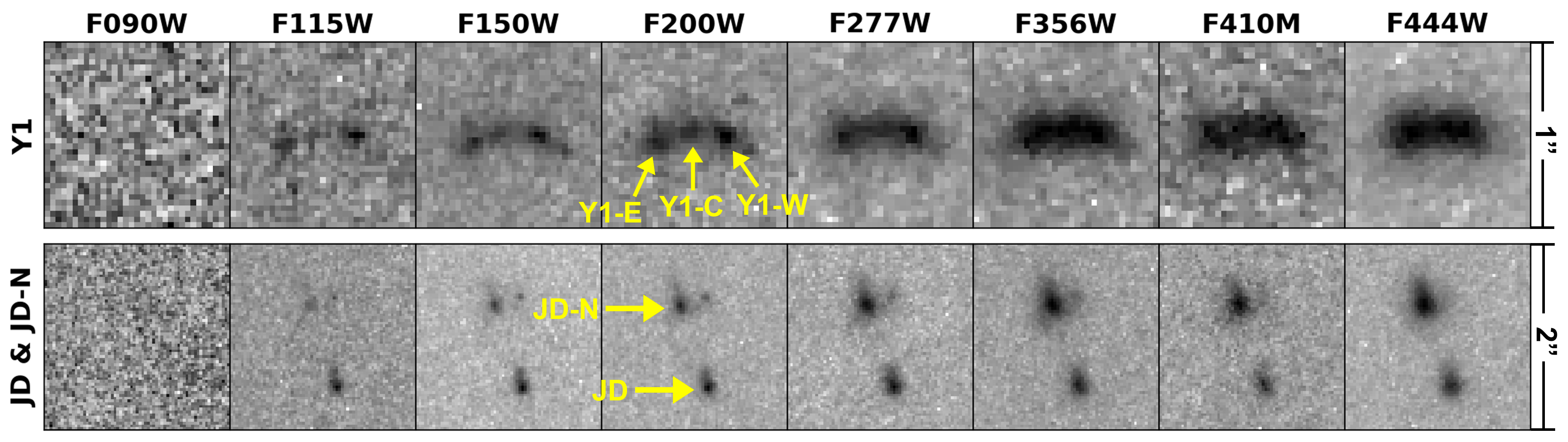
Figure 1: Cutouts of Y1 (top) and JD (bottom) in the eight NIRCam bands using the 30mas images. North is up and East is left. The size of the Y1 images is 1″$\times$1″, while that of the JD images is 2″$\times$2″. The three resolved Y1 components (Y1-E, Y1-C and Y1-W) are labeled in the F200W image. JD has a close companion, JD-N, whose colors also meet the requirements of a $J$-band dropout. Both objects are labeled in the F200W image.

2.1 NIRCam Imaging

MACS0416 is one of the targets observed by the JWST GTO program Prime Extragalactic Areas for Reionization and Lensing Science (PEARLS; PI: R. Windhorst; PID 1176; Windhorst et al. (2023)). It was imaged by NIRCam in eight filters, F090W, F115W, F150W, and F200W in the short wavelength channel (SW) and F277W, F356W, F410M, and F444W in the long wavelength channel (LW). The observations were carried out in three epochs: 2022 Oct 7 (Ep1), 2022 Dec 29 (Ep2), and 2023 Feb 10 (Ep3). The observations were described by Yan et al. (2023, their Table 1), who gave details of the data reduction. In Yan et al. (2023), the images were stacked on a per-epoch basis for the transient studies. For this work, we combined the data in all three epochs for JD, which reach the total integration times of 8761 seconds in F150W, F200W, F277W, and F356W, 10909 seconds in F115W and F410M, and 11338 seconds in F090W and F444W. In Ep3, Y1 is contaminated by a strong diffraction spike of a bright star, and therefore we only combined Ep1 and Ep2 data for the study of this object. The total integration times are 5841 seconds in F150W, F200W, F277W, and F356W, and 7559 seconds in F090W, F115W, F410M, and F444W, respectively. As Yan et al. (2023), we created stacks at scales of both 0$\farcs$06 (“60mas”) and 0$\farcs$03 (“30mas”), which have the magnitude zero point of 26.581 and 28.087, respectively. These images are all aligned to the HFF HST images.

2.2 NIRCam Wide-field Slitless Spectroscopy

MACS0416 was also observed by the NIRCam instrument in its wide-field slitless spectroscopy (WFSS) mode. This mode has two settings, Grism R and Grism C, which disperse light in either the direction of detector rows (“R”) or columns (“C”) in the LW channel, both having spectral resolution $R\approx 1600$ at $\sim$4 $\mu$m. The field was observed by the programs PID 2883 (“MAGNIF: Medium-band Astrophysics with the Grism of NIRCam in Frontier Fields,” PI: F. Sun) and PID 3538 (“Unveiling the properties of high-redshift low/intermediate-mass galaxies in Lensing fields with NIRCam Wide Field Slitless Spectroscopy,” PI: E. Iani).

The MAGNIF observations of MACS0416 were carried out on 2023 Aug 20 in Grism C using the F480M filter with total integration time of $\sim$3100 seconds. These observations covered only JD with Y1 $\sim$3″ outside the field. The observations of PID 3538 in this field were carried out on 2023 Dec 22–24 and 2024 Jan 17 in both Grisms R and C. Four filters were used, F300M, F335M, F410M, and F460M with total integration times in each band 1761 and 1546 seconds respectively for the two grisms.

To reduce the grism data, we retrieved the Level 1b “uncal” files from the Mikulski Archive for Space Telescopes (MAST) and ran them through the calwebb_detector1 routine of the JWST data reduction pipeline (version 1.13.4 under the context of jwst_1223.pmap) to obtain the “rate.fits” files. We then followed the procedures described by Sun et al. (2023) to further process the data. All single exposures were registered to the GAIA DR3 astrometry. There is a systematic offset between the HFF astrometry and that of GAIA in this field, which can be corrected by R.A.(GAIA) $=$ R.A.(HFF) $+$ 0$\farcs$21, and Decl.(GAIA) $=$ Decl.(HFF) $-$ 0$\farcs$08. This was taken into account when extracting the spectra.

3 Data Analysis

3.1 Overview

From their high-resolution (beam size 81.1$\times$112.2 mas) ALMA [O 3] 88 $\mu$m image of Y1, Tamura et al. (2023) resolved the system into three knots (“O1,” “O2,” and “O3”). Using this as a guide, these authors separated its HST WFC3 image into three components (“E,” “C,” and “W” from east to west) that coincide with the three [O 3] 88 $\mu$m knots. These three components are clearly distinguished in the NIRCam SW images (Figures 1 and 2), and the entire system extends $\sim$0$\farcs$73 along the long axis.

JD has a close companion object 0$\farcs$91 away to its northeast, which was also selected by Laporte et al. (2015) as a Y-band dropout (their “MACSJ0416.1_Y3”). As we will show below, its colors meet the requirements of a $J$-band dropout as well, and its redshift is nearly the same as that of JD. We refer to it as “JD-N” in this work to indicate its association with JD.

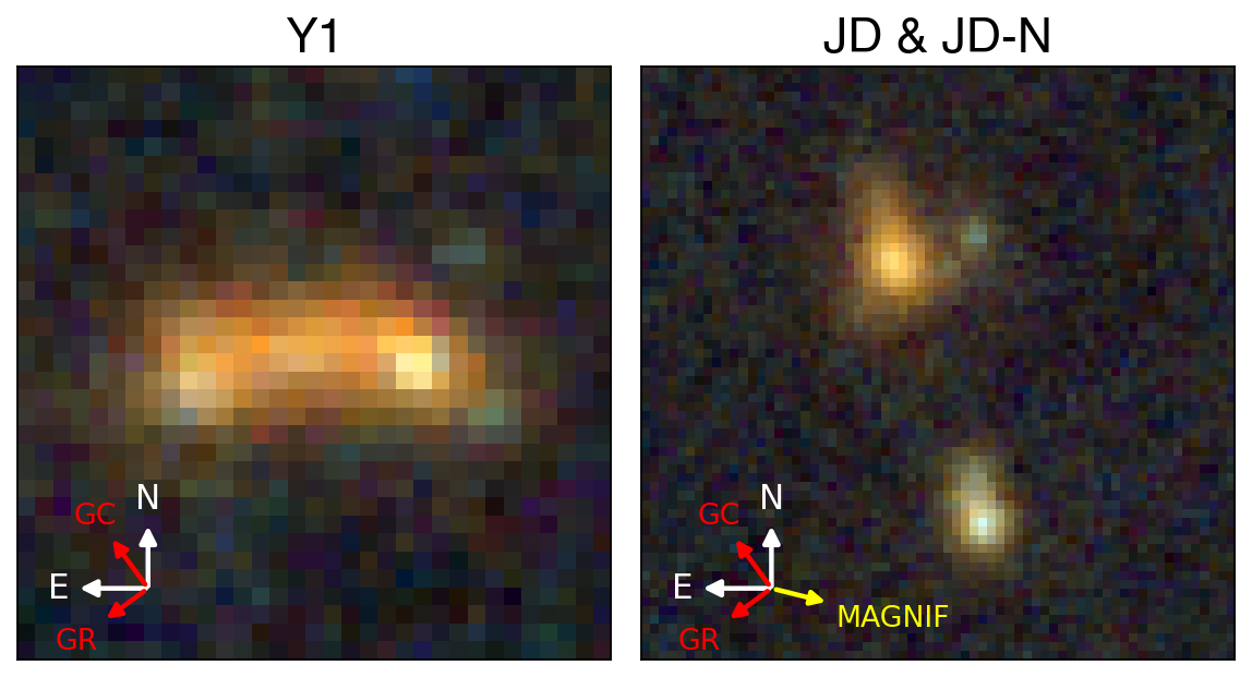
Figure 2: Color images of Y1 and JD, at the same scales as in Figure 1. The color scheme is F090W+F115W+F150W as blue, F200W+F277W as green, and F356W+F410M+F444W as red. In each image, the red arrows show the NIRCam grism WFSS dispersion direction in the PID 3538 observation in Grism C (GC) and Grism R (GR), respectively; the yellow arrow in the JD image shows the dispersion direction of GC utilized by the MAGNIF observations.

3.2 Photometry and SEDs

To construct the SEDs of our targets, we used the photometry on the 60mas images. These images were convolved to match their point spread functions (PSFs) to that of the F444W image, which has the coarsest spatial resolution (PSF full width at half-maximum, or FWHM, 0$\farcs$145). WebbPSFs (Perrin et al., 2014, 2015) were used in the convolution. Matched-aperture photometry was done by running SExtractor (Bertin & Arnouts, 1996) in the dual-image mode with F444W as the detection band, and we adopted the MAG_ISO magnitudes.

We obtained SEDs for Y1’s three components using the 30mas images. As they are severely blended, they cannot be separated automatically. Therefore, we manually defined the segmentation map for the three components based on the 30mas F200W image, where they are the most clearly detected and separated. With this segmentation map (illustrated in Figure 3), we used Photutils (Bradley et al., 2023) to extract the flux for each component in each band on the PSF-matched 60mas images.

Table 1 summarizes the photometry for all these sources. From their colors (large magnitude breaks between F115W and F150W and being ${\rm S/N}<2$ in F090W), JD and JD-N indeed qualify as $J$-band dropouts.

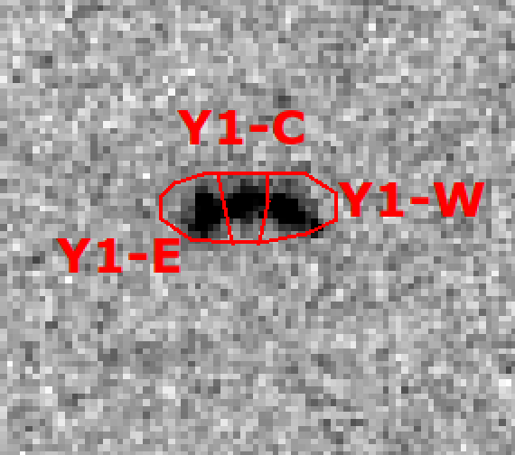
Figure 3: Illustration of the Y1 segmentation (in red polygons) that separate its three components for individual flux extraction in the imaging data. The background is the 30mas F200W image.

Table 1: NIRCam photometry (without correcting for lensing magnification)

	Y1	Y1-E	Y1-C	Y1-W	JD	JD-N
R.A. (deg)	64.0391682	64.0392323	64.0391780	64.0391192	64.0479851	64.0480694
Decl (deg)	-24.0931764	-24.0931976	-24.0931800	-24.0931886	-24.0816685	-24.0814279
F090W	$>$29.96	$>$29.96	$>$29.96	$>$29.96	30.41 $\pm$ 2.54	30.29 $\pm$ 2.78
F115W	26.89 $\pm$ 0.15	28.39 $\pm$ 0.09	28.68 $\pm$ 0.11	28.17 $\pm$ 0.08	27.66 $\pm$ 0.21	27.71 $\pm$ 0.26
F150W	26.14 $\pm$ 0.07	27.56 $\pm$ 0.04	27.69 $\pm$ 0.04	27.37 $\pm$ 0.04	26.65 $\pm$ 0.08	26.52 $\pm$ 0.09
F200W	26.07 $\pm$ 0.06	27.51 $\pm$ 0.04	27.54 $\pm$ 0.03	27.29 $\pm$ 0.03	26.85 $\pm$ 0.08	26.43 $\pm$ 0.07
F277W	25.96 $\pm$ 0.02	27.53 $\pm$ 0.01	27.43 $\pm$ 0.01	27.26 $\pm$ 0.01	26.97 $\pm$ 0.03	26.30 $\pm$ 0.02
F356W	25.58 $\pm$ 0.01	27.27 $\pm$ 0.01	27.15 $\pm$ 0.01	27.06 $\pm$ 0.01	26.91 $\pm$ 0.03	25.94 $\pm$ 0.01
F410M	25.90 $\pm$ 0.03	27.57 $\pm$ 0.02	27.41 $\pm$ 0.02	27.28 $\pm$ 0.02	27.06 $\pm$ 0.05	25.96 $\pm$ 0.03
F444W	24.84 $\pm$ 0.01	26.58 $\pm$ 0.01	26.30 $\pm$ 0.01	26.34 $\pm$ 0.01	26.22 $\pm$ 0.02	25.32 $\pm$ 0.01

3.3 Spectroscopic Identifications

Figure 2 shows the color composites of these two systems, where the WFSS dispersion directions are indicated. The NIRCam WFSS mode is very suitable for the detection of emission lines, which is the main focus here. To optimize the line detection, we subtracted a continuum estimated (following Kashino et al. 2023) by running a median filter $1\times 51$ pixels in size with a 9-pixel “hole” at the center along each row or column.

As Y1 consists of three components, it would be ideal to extract the spectra for each component. In practice, however, the individual extraction could only split the signal into two parts, which largely coincide with Y1-E and Y1-W, respectively. This is due to both the faintness of Y1-C at 3–5 $\mu$m and the coarse resolution at these wavelengths. For simplicity, we refer to the separate extractions as Y1-E and Y1-W even though both could include some contribution from Y1-C. As shown in Figure 2, the PID 3538 Grism R dispersion direction is very close to the spatial extension of the Y1 system, causing severe spectral contamination between the two components. For this reason, we only used the Grism C data. The extracted 2D and 1D spectra are shown in Figure 4.

For both Y1-E and Y1-W, the [O 3] $\lambda\lambda$4959,5007 lines are clearly seen in the F460M data. The detection of the [O 2] $\lambda$3727 line in the F335M data is marginal in the 1D spectrum but convincing in the 2D spectrum. To determine the redshifts, we fitted a Gaussian profile to the [O 3] $\lambda$5007 line, which is the strongest, to obtain its observed central wavelengths. The redshifts thus derived are $z=8.309\pm 0.002$ for Y1-E and $z=8.312\pm 0.002$ for Y1-W. We also fitted Gaussians to the weaker lines, using the initial guesses of the line centers at where they should be under these redshifts. The results based on the best-fit central wavelengths thus obtained are all in excellent agreement with the redshifts based on the [O 3] $\lambda$5007 line.

For JD and JD-N, we extracted the spectra using the data from both MAGNIF and PID 3538. However, we discarded the Grism C data from the latter because its dispersion direction is almost parallel to the position angle of the two objects (Figure 2). The spectra are shown in Figure 4. JD-N shows two lines, one strong and the other marginal, in the F460M data from PID 3538 Grism R. Based on Gaussian fitting as above, these two lines coincide with the [O 3] $\lambda\lambda$4959,5007 doublet at $z=8.346\pm 0.002$. The MAGNIF F480M Grism C data reveal only one line, which should be [O 3] $\lambda$5007. The [O 3] $\lambda$4959 line falls outside the filter transmission range and is not detected. For JD, the data from both programs show only one strong line. Given its possible redshift range, the line must be [O 3] $\lambda$5007 at $z=8.341\pm 0.002$. The non-detection of the [O 3] $\lambda$4959 line in the MAGNIF data is again because it is outside of the filter transmission range. On the other hand, the non-detection of the $\lambda$4949 line in the PID 3538 is likely because of limited sensitivity: given the expected ratio of $\sim$1:3 of the [O 3] doublet, the [O 3] $\lambda$4959 line flux is comparable to the noise level of the data.

Table 2 summarizes the line measurements. The line widths were converted to velocities by $\Delta v=c\Delta\lambda/\lambda_{c}$, where $\lambda_{c}$ and $\Delta\lambda$ are the mean and FWHM of the Gaussian fit, respectively, and $c$ is the speed of light. The total line intensities were obtained by integrating the fitted Gaussian profile within a $4\times$FWHM wavelength range centered at $\lambda_{c}$. The associated errors were estimated using the non-smoothed 1D spectra. When calculating the observed equivalent widths (EW), the F410M magnitudes in Table 1 were used as the continuum flux density. To account for continuum contributions from Y1-C in the spectra of Y1-E and Y1-W, half the F410M flux density of Y1-C was added to the Y1-E and Y1-W continua. Not surprisingly, these objects all have very large [O 3] EW values, which can largely account for the brightening of their SEDs in F444W. For example, the measured [O 3] $\lambda$5007 EW of JD implies that this line alone increases the object’s F444W brightness (as compared to that in F410M) by $-0.83\pm 0.06$ mag, which is almost the same as the observed $m_{410}-m_{444}=-0.84\pm 0.05$ mag.

Table 2: Summary of NIRCam WFSS results

Target	Program	Grating	$z$	$I_{5007}$	$\Delta v_{5007}$	EW5007	$I_{4959}$	$\Delta v_{4959}$	EW4959	$I_{3727}$	$\Delta v_{3727}$	EW3727
Y1-E	3538	F335M+F460M/C	8.309±0.002	1.10±0.12	338±26	14879±1221	0.43±0.07	366±91	5727±733	0.18±0.08	541±171	1338±542
Y1-W	3538	F335M+F460M/C	8.312±0.002	1.11±0.10	310±32	12519±913	0.45±0.11	346±78	4967±848	0.24±0.10	424±71	1505±310
JD	MAGNIF	F480M/C	8.339±0.002	0.55±0.12	249±35	7394±1805	…	…	…	…	…	…
	3538	F460M/R	8.341±0.002	0.64±0.10	217±23	8635±1124	…	…	…	…	…	…
JD-N	MAGNIF	F480M/C	8.346±0.002	1.13±0.11	274±35	5479±423	…	…	…	…	…	…
	3538	F460M/R	8.346±0.002	1.09±0.12	316±20	5325±356	0.39±0.15	409±91	1870±442	…	…	…

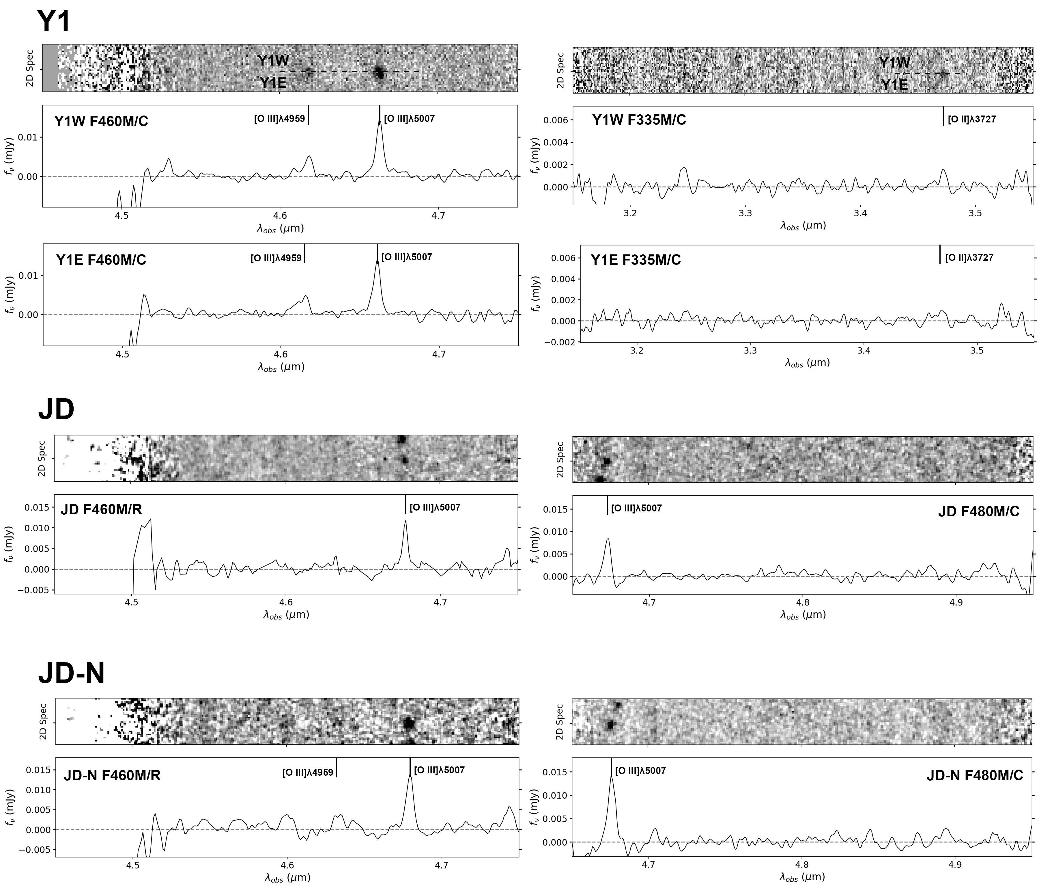
Figure 4: Extracted 2D and 1D spectra from the NIRCam WFSS observations. For each object, the top panel shows the 2D spectrum with background and continuum subtracted, and the bottom panel shows the resultant 1D spectrum and includes the object label. Identified emission lines are marked. The 2D spectra of JD and JD-N are displayed after smoothing with a Gaussian kernel with $\sigma=1$, while the 1D spectra are based on the unsmoothed 2D spectra, then smoothed using a Gaussian kernel with $\sigma=0.6$. The 2D spectra of Y1 are not smoothed to show the separation of the two components, but the 1D spectra are smoothed with $\sigma=0.6$. With only a few exposures in each setup, stacking has limited ability to remove outlying pixels, leaving some narrow spikes in the 1D spectra. Fortunately, the emission lines of interest are not contaminated by such spikes.

4 Discussion

4.1 Redshifts, environment, and magnification

The redshifts of Y1-E and Y1-W agree with each other within the uncertainties, and their rest-frame relative velocity is only $97\pm 64$ km s^-1. The average is $z=8.311\pm 0.003$, which is in very good agreement with the previously reported $z=8.3118\pm 0.0003$ based on [O 3] 88 $\mu$m (Tamura et al., 2019) and $z=8.31132\pm 0.00037$ based on [C 2] 157.5 $\mu$m (Bakx et al., 2020) for Y1. The apparent [O 3] 88 $\mu$m line flux measured by (Tamura et al., 2019) is 0.66 Jy km s^-1, which corresponds to $7.92\times 10^{-18}$ erg cm^-2 s^-1 at the observed frequency (364.377 GHz). Therefore, the line flux ratio of [O 3] $\lambda$5007 and 88 $\mu$m is 2.79.

For JD, our redshift of $z=8.341\pm 0.002$ disagrees with the previously reported $z=9.28$ by Laporte et al. (2021), which was based on their claimed detection of the [O 3] 88 $\mu$m line. That redshift would give no obvious identification for the emission line observed at 4.68 µm. We have reduced the same ALMA Band 7 data used by these authors but do not detect a line (Appendix A). At $z=8.346\pm 0.002$, the velocity offset from JD to JD-N is $160\pm 64$ km s^-1.

According to the lens model of Diego et al. (2023), the magnification factors for Y1 and JD/JD-N are $\mu=1.21$ and 2.26, respectively. Based on their magnitudes in F150W (sampling the rest-frame UV range of $\sim$1430–1790Å at these redshifts), their intrinsic absolute UV magnitudes after correcting the lensing magnifications are $M_{\rm UV}=-20.85$, $-19.66$ and $-19.80$ mag for Y1, JD, and JD-N, respectively. The observed size of Y1 as a whole is only marginally affected by the magnification, and its corresponding physical size along the long axis is $\sim$3.4 kpc. The separation of JD and JD-N, on the other hand, is affected significantly by lensing. Their separation in the source plane is $\sim$0$\farcs$51, which corresponds to 2.4 kpc. Therefore, JD and JD-N very likely form a interacting pair.

4.2 Stellar populations

To understand the stellar populations of these galaxies, we fitted their SEDs using the Bagpipes software (Carnall et al., 2018), which utilizes the stellar population synthesis models of Bruzual & Charlot (2003) with the Kroupa (2001) initial mass function. The fitting was done at fixed redshifts of 8.31 and 8.34 for Y1 and JD/JD-N, respectively. An exponentially declining star formation history (SFH) in the form of SFR $\propto e^{-t/\tau}$ was adopted. The option to include nebular emission lines was enabled, and we used the Calzetti dust-extinction law (Calzetti et al., 1994; Calzetti, 2001) with $A_{V}$ ranging from 0 to 2.0 mag. The metallicity was allowed in the range of $0\leq Z_{*}/Z_{\odot}\leq 2.5$, and the ionization parameter could vary in $-2.5<{\rm log}(U)<-0.5$. The results of the SED fitting are summarized in Table 3, and Figure 5 shows the 16th to 84th percentile range for the posterior spectra superposed on the SEDs. The “corner plots” showing the posterior for fitted parameters are given in Figure 6. Overall, Y1, JD, and JD-N have rather similar physical properties, and the three components of Y1 are also quite similar to each other.

The existence of the oxygen lines in these objects (as well as the [C 2] 157.7 $\mu$m line in Y1) indicates that they have already acquired a substantial amount of metals, and this is further supported by the metallicities dervied from the SED analysis ($Z/Z_{\odot}\approx 0.4$–0.6). Interestingly, all the objects are $\lesssim 11$ Myr old, which means that the only route for their metal enrichment was through core-collapse supernovae. Consistent with their young ages, the galaxies have low stellar masses of 0.8–6.4 $\times 10^{8}\leavevmode\nobreak\ {\rm M_{\odot}}$ (after correcting for lensing magnifications), which can be achieved by SFRs on the order of a few tens to $\sim$100 ${\rm M_{\odot}}$ yr^-1 as derived (see also Figure 6).

Table 3: Bagpipes posterior parameters of the fitted stellar populations

Object	$A_{V}$	Age/Myr	$Z/Z_{\sun}$	${\rm log}(U)$	${\rm log}(\mu M/\mathrm{M_{\sun}})$	$\mu$SFR/($\mathrm{M_{\odot}\ yr}^{-1}$)
Y1	$0.80^{+0.06}_{-0.11}$	$2.68^{+0.81}_{-1.09}$	$0.60^{+0.19}_{-0.30}$	$-2.04^{+0.09}_{-0.15}$	$8.89^{+0.06}_{-0.14}$	$291.69^{+299.73}_{-127.88}$
Y1-E	$0.85^{+0.08}_{-0.11}$	$2.86^{+1.08}_{-1.15}$	$0.60^{+0.21}_{-0.25}$	$-1.73^{+0.13}_{-0.22}$	$8.27^{+0.08}_{-0.14}$	$63.09^{+72.83}_{-27.12}$
Y1-C	$0.95^{+0.07}_{-0.08}$	$2.44^{+0.68}_{-0.96}$	$0.57^{+0.15}_{-0.17}$	$-1.62^{+0.12}_{-0.13}$	$8.37^{+0.07}_{-0.07}$	$107.42^{+65.41}_{-37.10}$
Y1-W	$0.95^{+0.09}_{-0.16}$	$3.32^{+1.24}_{-1.53}$	$0.58^{+0.30}_{-0.24}$	$-1.43^{+0.22}_{-0.21}$	$8.46^{+0.12}_{-0.16}$	$87.19^{+112.34}_{-44.32}$
JD	$0.41^{+0.13}_{-0.20}$	$3.57^{+1.09}_{-1.63}$	$0.44^{+0.35}_{-0.18}$	$-1.02^{+0.34}_{-0.35}$	$8.26^{+0.16}_{-0.19}$	$51.37^{+86.37}_{-25.17}$
JD-N	$0.94^{+0.10}_{-0.10}$	$11.47^{+2.20}_{-1.88}$	$0.36^{+0.13}_{-0.08}$	$-1.99^{+0.17}_{-0.12}$	$8.96^{+0.06}_{-0.08}$	$80.23^{+22.97}_{-13.55}$

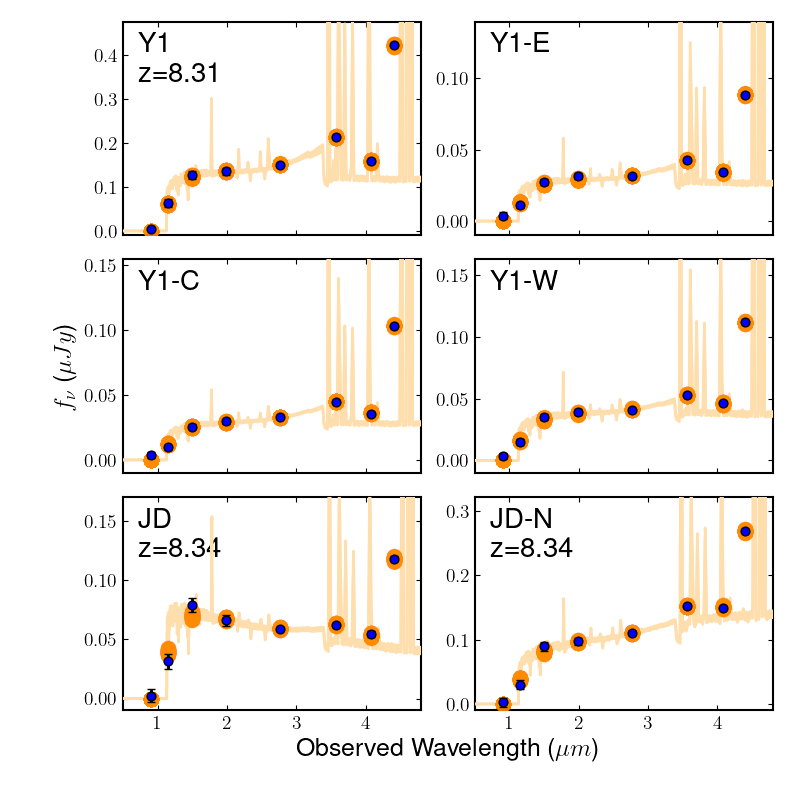
Figure 5: Illustration of the SED fitting with Bagpipes for each entry in Table 1. The blue points with error bars show the observed flux densities, and the orange points show the synthesized magnitudes from the 50th-percentile Bagpipes fit. The posterior spectra corresponding to the 16th and 84th percentile range are shown in yellow in each panel.

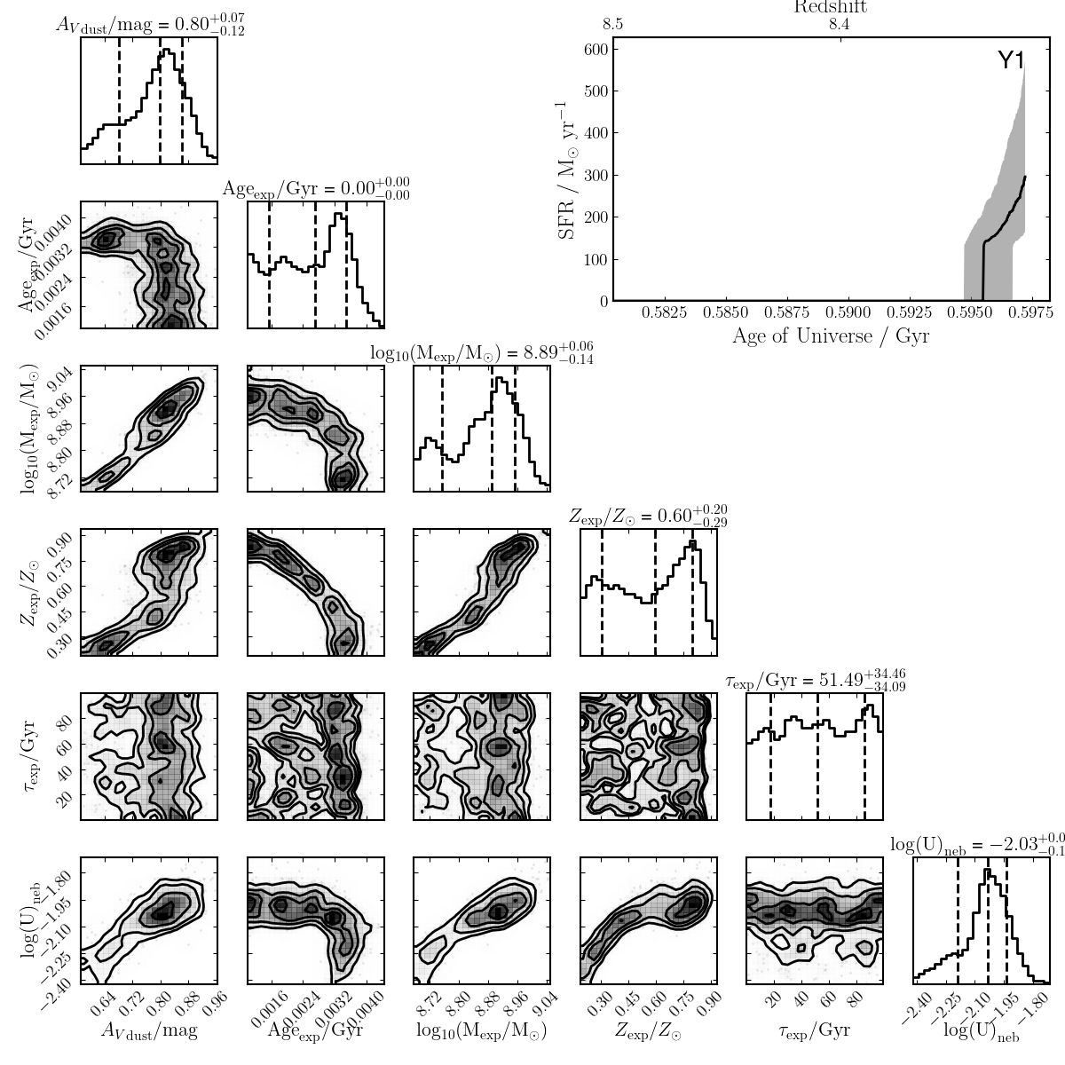
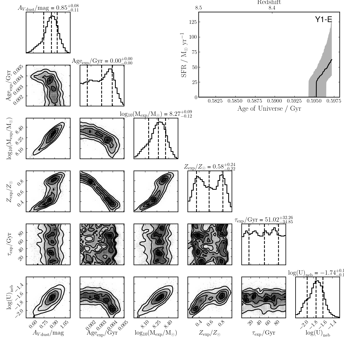
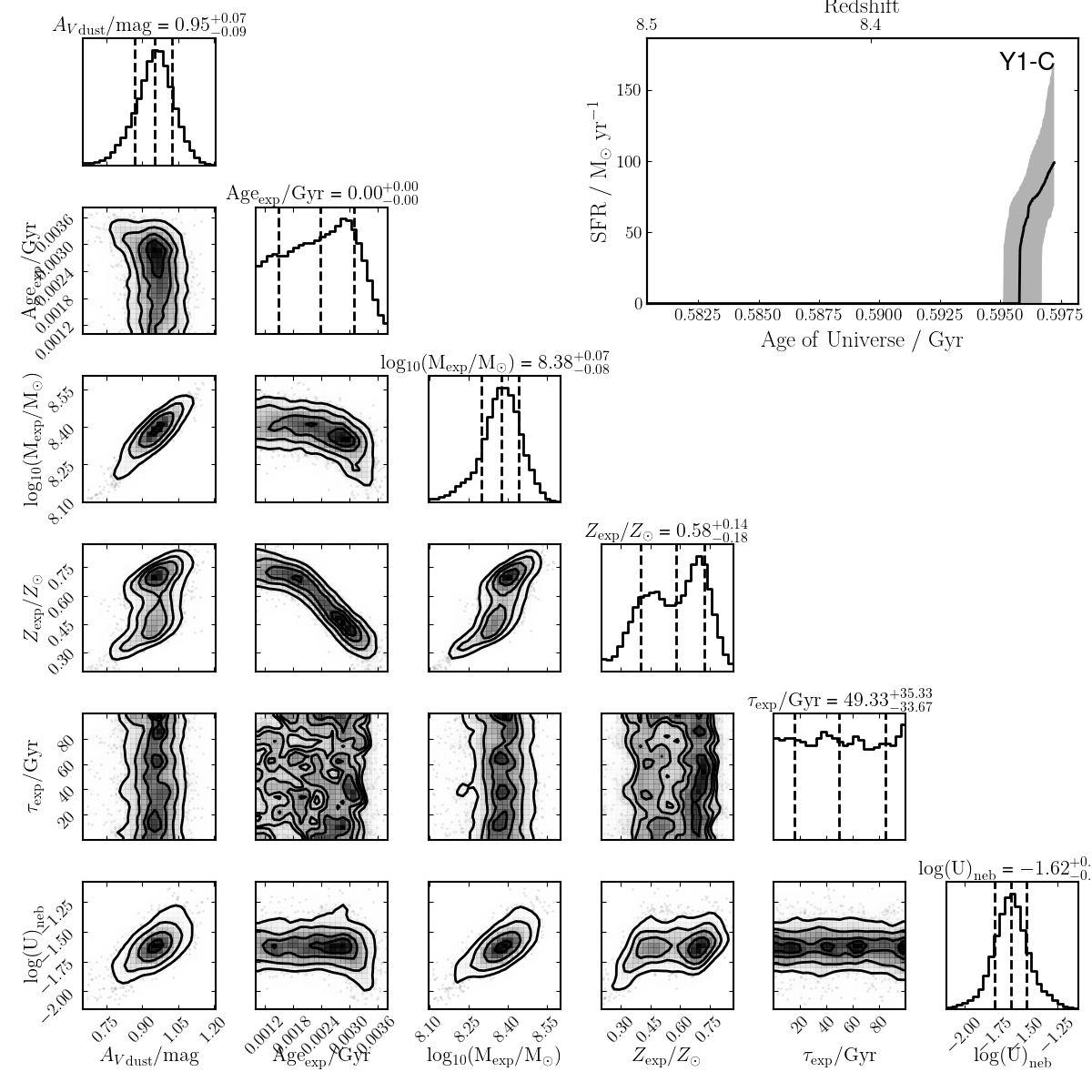
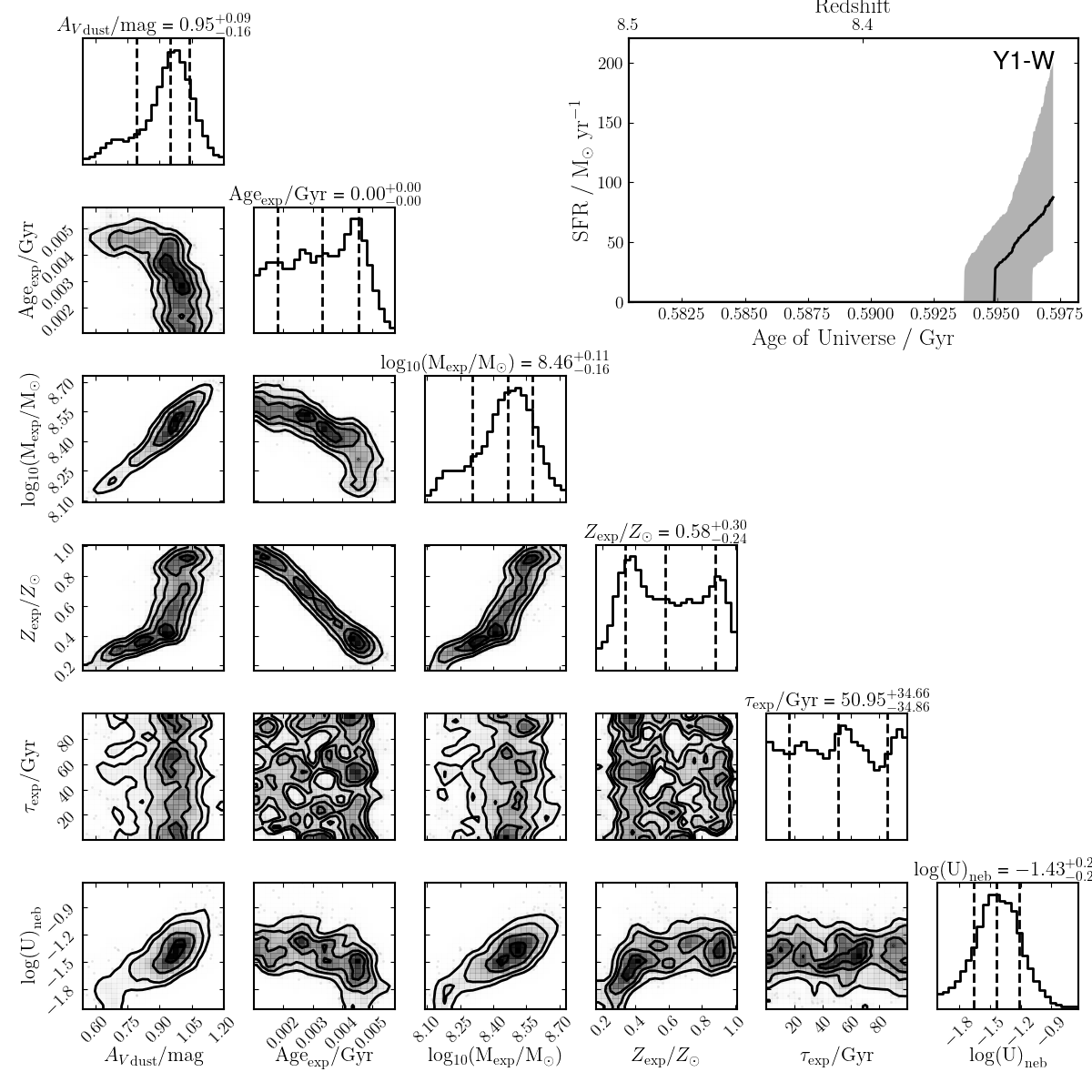
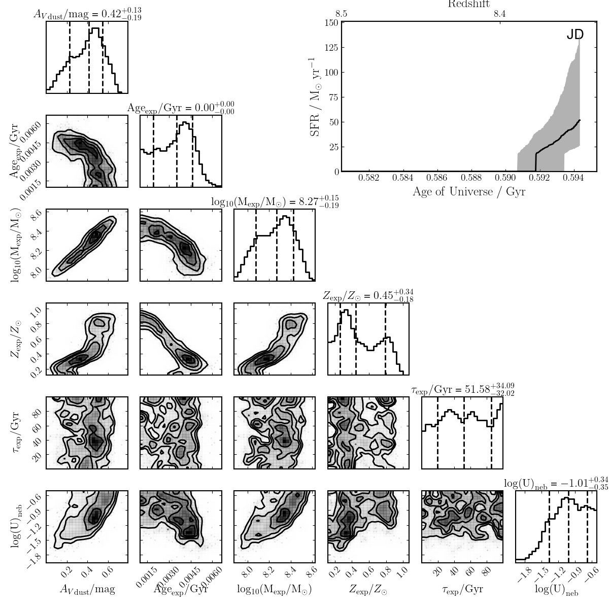
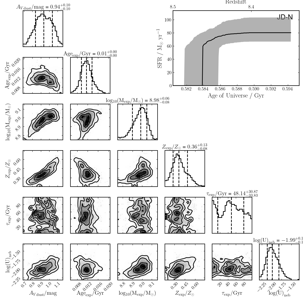
Figure 6: Corner plots showing the posterior distributions of the fitted parameters corresponding to the SED fitting illustrated in Figure 5. The inset in the upper right corner in each panel shows the SFH, where the shaded region corresponds to the 16th to 84th percentile range, and the black curve is the median value.

Table 4: Rest-frame UV slopes and $f_{\rm esc}$

Name	$\beta^{150,200}$	$f_{\rm esc}^{150,200}$	$\beta^{150,277}$	$f_{\rm esc}^{150,277}$	$\beta^{\rm PL}$	$f_{\rm esc}^{\rm PL}$
Y1	$-$1.769	0.019	$-$1.731	0.017	$-$1.417	0.007
Y1-E	$-$1.838	0.023	$-$1.955	0.032	$-$1.304	0.005
Y1-C	$-$1.515	0.009	$-$1.610	0.012	$-$1.200	0.004
Y1-W	$-$1.761	0.018	$-$1.834	0.022	$-$1.206	0.004
JD	$-$2.630	0.210	$-$2.479	0.138	$-$1.967	0.033
JD-N	$-$1.718	0.016	$-$1.673	0.014	$-$1.204	0.004

4.3 UV slopes and Lyman-continuum photon escape fractions

Using the photometry reported in Table 1, we calculated the rest-frame UV slope $\beta$ for these sources. The calculation was done using two different filter pairs, (F150W, F200W) and (F150W, F277W), which approximately correspond to using the rest-frame wavelength pairs of (1600Å, 2100Å) and (1600Å, 3000Å), respectively. As an alternative, we also used the best-fit template spectrum (corresponding to the 50th percentile of the posterior distribution) of the SED and fitted a power law between 1300Å and 1850Å in the rest-frame to obtain this slope. These results are listed in Table 4. The slopes derived using the best-fit template spectra ($\beta^{\rm PL}$) are all significantly flatter than those obtained using the photometry in the blue passband pairs ($\beta^{150,200}$ and $\beta^{150,277}$), which cautions that care must be taken when interpreting UV slopes obtained by different methods (e.g., Dunlop et al., 2013; Austin et al., 2024). The UV slopes are related to the Lyman continuum photon escape fractions ($f_{\rm esc}$), which are critical in understanding the sources of the cosmic hydrogen reionization. For each $\beta$ value, we calculated $f_{\rm esc}$ following Equation 11 of Chisholm et al. (2022),

$$f_{\rm esc}=(1.3\pm 0.6)\times 10^{-4}\cdot 10^{(-1.22\pm 0.1)\beta}\,.$$ (1)

The derived values are reported in Table 4.

Somewhat surprisingly, only JD has a blue slope of $\beta\lesssim-2.0$, and its inferred $f_{\rm esc}$ ranges from $\sim$3.3% to 21.0% depending on the exact $\beta$ value adopted. In terms of their stellar populations, the three objects are quite similar to each other, and the only major difference is that JD has only half as much reddening ($A_{\rm V}\sim 0.4$ mag) as Y1 and JD-N ($\sim$0.8–0.9 mag). This should be the main factor that affects their UV slopes and hence their $f_{\rm esc}$. This also suggests that a significant fraction of very young galaxies at high redshifts might not contribute to reionization because they formed a considerable amount of dust that dispersed throughout their bodies in only a few Myr.

5 Summary

New JWST data show that three $z\approx 8.3$ galaxies behind the lensing cluster MACS0416 are strong [O 3] $\lambda$5007 emitters. Their line equivalent widths can easily explain their apparent flux excess in F444W. Two galaxies, Y1 and JD, had prior spectroscopic redshifts through ALMA detections of the [O 3] 88 $\mu$m line and/or [C 2] 157.7 $\mu$m line for JD. We confirm the redshift 8.31 for Y1 but find $z=8.34$ for JD as opposed to the previously claimed $z=9.28$. Y1 is a merging system and is resolved into three components extending $\sim$3.4 kpc along the long axis. The three components all have very similar properties. The third object, JD-N, is a previously discovered candidate at $z\approx 8$ and is now confirmed to have the same redshift as JD; the two are only $\sim$0$\farcs$51 ($\sim$2.4 kpc) apart in the source plane and therefore very likely merging or at least interacting. These three objects are magnified by only a moderate amount and have intrinsic $M_{\rm UV}$ ranging from $-19.66$ to $-20.85$ mag. Our SED analysis show that they are all very young systems in the making, with ages $\lesssim$11 Myr, arguably the youngest galaxies ever reported at $z>6$. Their stellar masses are on the order of $10^{8}$ ${\rm M_{\odot}}$. They are actively forming stars, with SFRs of a few tens to a couple of hundred $\rm{M_{\odot}}$ yr^-1. However, only JD has a blue rest-frame UV slope ($\beta$ ranging from $-1.97$ to $-2.63$ depending on how it is derived), indicative of a high Lyman-continuum photon escape fraction ($f_{\rm esc}$ could be as high as 21%). In contrast, Y1 and JD-N have $\beta\lesssim-1.7$ – $-1.8$, implying $f_{\rm esc}\lesssim 3\%$ despite their higher SFRs than JD, due to their twice as high dust extinction. This suggests that even very young, very actively star-forming galaxies at high-$z$ could have negligible contribution to the ionizing background if they form dust throughout their bodies too quickly (over a few Myr time scale). Y1 and JD-N are examples that dust formation and pollution processes at $z>8$ could indeed be very fast.

Appendix A Null line detection in the ALMA data for JD

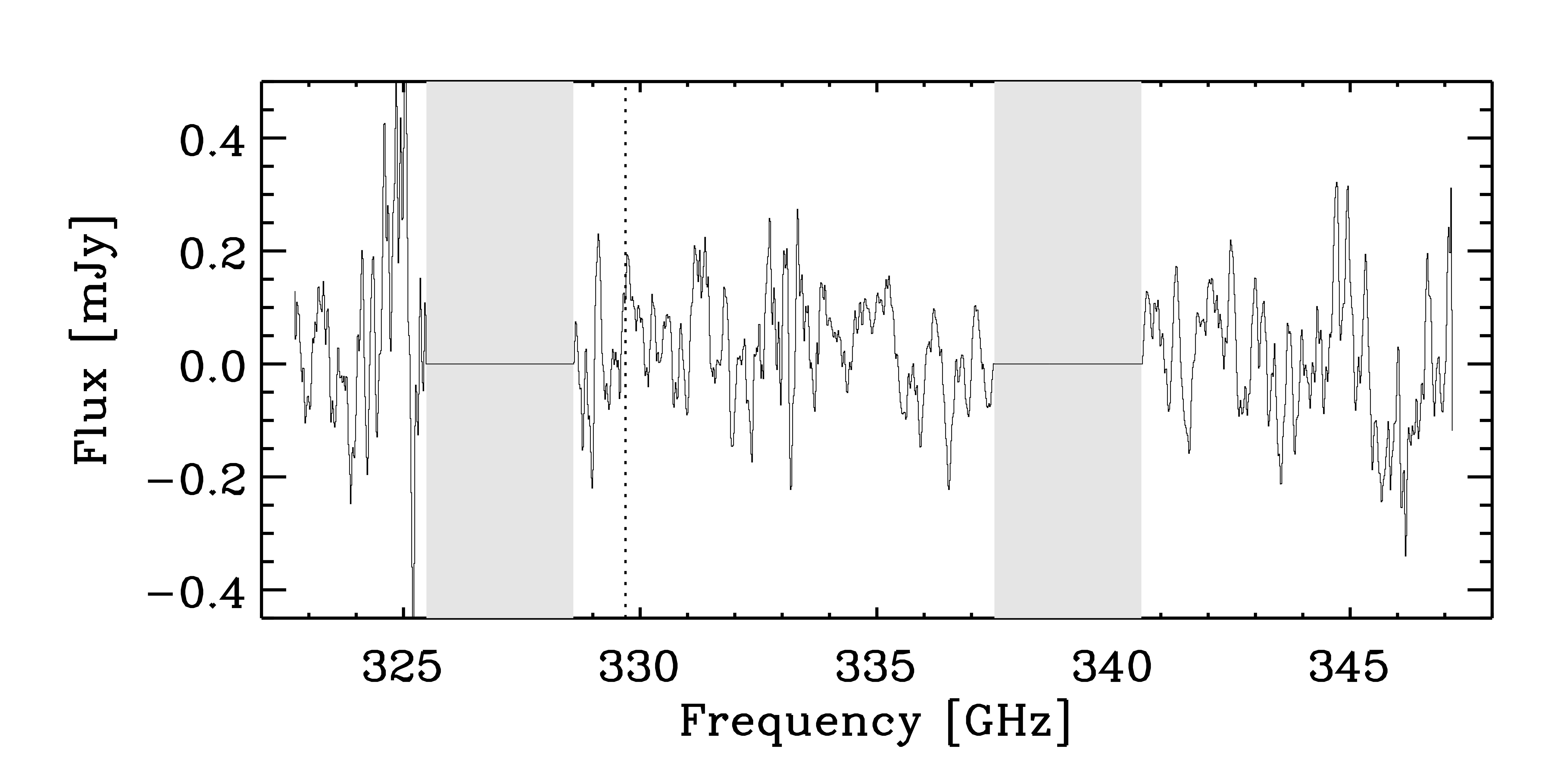
Figure A.1: Spectrum of JD from the ALMA Band 7 data based on our own reduction. The grey regions indicate frequency ranges not covered by the observations. The spectrum was extracted at the position shown in Figure 2 of Laporte et al. (2021) using an aperture of 1$\farcs$00$\farcs$35 in diameter. The dashed vertical line indicates 329.69 GHz, where Laporte et al. (2021) claimed a line detection.

We reduced the same ALMA band 7 data of JD (PID: 2019.1.00061.S, PI: R. Ellis) used by Laporte et al. (2021). We utilized the default ALMA data reduction script ScriptForPi.py to obtain the visibility file and performed tclean in the Common Astronomy Software Applications package (CASA). The cleaning was done using natural weighting and frequency bin 16 MHz. The final cube has an rms of 0.23 mJy beam^-1. We extracted the spectrum at the position shown by (Laporte et al., 2021, their Figure 2) with an aperture of 1$\farcs$0 in diameter, and the result is shown in Figure A.1. No emission line is detected at the frequency where Laporte et al. (2021) saw a detection.

Appendix B Age estimates using different SFHs

For a given stellar population synthesis model, the age estimate could be affected by the adopted SFH. The SED analysis presented in Section 4.2 uses an exponentially declining SFH, also known as the “$\tau$ model”. To test the robustness of the very young ages thus obtained, we also ran Bagpipes using some other SFHs offered with the package:

• Delayed $\tau$:

  $$\quad\mathrm{SFR}(t)\ \propto\ \begin{cases}\ \ \ (t-T_{0})\ \mathrm{exp}\bigg{(}-\dfrac{t-T_{0}}{\tau}\bigg{)}&\quad t>T_{0}\\ \ \ \ 0&\quad t<T_{0}.\end{cases}$$ (B1)

• Log-normal:

  $$\mathrm{SFR}(t)\ \propto\ \frac{1}{t}\ \mathrm{exp}\bigg{(}-\frac{\big{(}\mathrm{ln}(t)-T_{0}\big{)}^{2}}{2\tau^{2}}\bigg{)}$$ (B2)

• Double power law:

  $$\mathrm{SFR}(t)\ \propto\ \Bigg{[}\bigg{(}\frac{t}{\tau}\bigg{)}^{\alpha}+\bigg{(}\frac{t}{\tau}\bigg{)}^{-\beta}\Bigg{]}^{-1}$$ (B3)

Table B.1 compares the best-fit stellar mass and age parameters obtained using the $\tau$ model with those obtained using these alternative SFHs. For both the $\tau$ and the delayed $\tau$ models, the age parameter is among the direct outputs. This is not the case when using the log-normal or the double power law models, however, because there is no clear definition of age in either SFH. To obtain an estimate in these two cases, we derived an age proxy denoted as ${\rm Age_{N}}$, which is the time for the galaxy to gain 100% of its stellar mass starting from the time when it had N% of its total stellar mass. For the demonstration purpose here, $N$ was set to 10, 50, and 90. As shown by this comparison, these alternative SFHs resulted in comparable, young ages for all three objects.

Table B.1: Comparison of best-fit galaxy properties with different SFH

		Exponential	Delayed $\tau$	Log-norm	Double PL
Y1	${\rm log}(\mu M/\mathrm{M_{\sun}})$	$8.89^{+0.06}_{-0.14}$	$8.86^{+0.09}_{-0.11}$	$8.80^{+0.06}_{-0.07}$	$8.82^{+0.07}_{-0.01}$
	Age/Myr	$2.68^{+0.81}_{-1.09}$	$4.15^{+1.04}_{-2.19}$	…	…
	Age10/Myr	…	…	3.75	3.62
	Age50/Myr	…	…	1.29	1.70
	Age90/Myr	…	…	1.00	1.00
JD	${\rm log}(\mu M/\mathrm{M_{\sun}})$	$8.26^{+0.16}_{-0.19}$	$8.28^{+0.15}_{-0.16}$	$8.19^{+0.12}_{-0.13}$	$8.24^{+0.12}_{-0.11}$
	Age/Myr	$3.57^{+1.09}_{-1.63}$	$4.96^{+2.27}_{-2.53}$	…	…
	Age10/Myr	…	…	6.46	3.30
	Age50/Myr	…	…	2.16	1.43
	Age90/Myr	…	…	1.00	1.00
JD-N	${\rm log}(\mu M/\mathrm{M_{\sun}})$	$8.96^{+0.06}_{-0.08}$	$9.00^{+0.06}_{-0.07}$	$9.05^{+0.06}_{-0.08}$	$8.99^{+0.06}_{-0.08}$
	Age/Myr	$11.47^{+2.20}_{-1.88}$	$24.39^{+5.2}_{-5.77}$	…	…
	Age10/Myr	…	…	20.40	15.22
	Age50/Myr	…	…	6.28	5.72
	Age90/Myr	…	…	1.01	1.02

References

- Austin et al. (2024) Austin, D., Conselice, C. J., Adams, N. J., et al. 2024, arXiv e-prints, arXiv:2404.10751, doi: 10.48550/arXiv.2404.10751
- Bakx et al. (2020) Bakx, T. J. L. C., Tamura, Y., Hashimoto, T., et al. 2020, MNRAS, 493, 4294, doi: 10.1093/mnras/staa509
- Bertin & Arnouts (1996) Bertin, E., & Arnouts, S. 1996, A&AS, 117, 393, doi: 10.1051/aas:1996164
- Bouwens et al. (2006) Bouwens, R. J., Illingworth, G. D., Blakeslee, J. P., & Franx, M. 2006, ApJ, 653, 53, doi: 10.1086/498733
- Bouwens et al. (2010) Bouwens, R. J., Illingworth, G. D., Oesch, P. A., et al. 2010, ApJ, 708, L69, doi: 10.1088/2041-8205/708/2/L69
- Bradley et al. (2023) Bradley, L., Sipőcz, B., Robitaille, T., et al. 2023, astropy/photutils: 1.8.0, 1.8.0, Zenodo, doi: 10.5281/zenodo.7946442
- Bruzual & Charlot (2003) Bruzual, G., & Charlot, S. 2003, MNRAS, 344, 1000, doi: 10.1046/j.1365-8711.2003.06897.x
- Calzetti (2001) Calzetti, D. 2001, PASP, 113, 1449, doi: 10.1086/324269
- Calzetti et al. (1994) Calzetti, D., Kinney, A. L., & Storchi-Bergmann, T. 1994, ApJ, 429, 582, doi: 10.1086/174346
- Carnall et al. (2018) Carnall, A. C., McLure, R. J., Dunlop, J. S., & Davé, R. 2018, MNRAS, 480, 4379, doi: 10.1093/mnras/sty2169
- Chisholm et al. (2022) Chisholm, J., Saldana-Lopez, A., Flury, S., et al. 2022, MNRAS, 517, 5104, doi: 10.1093/mnras/stac2874
- Coe et al. (2015) Coe, D., Bradley, L., & Zitrin, A. 2015, ApJ, 800, 84, doi: 10.1088/0004-637X/800/2/84
- Coe et al. (2019) Coe, D., Salmon, B., Bradač, M., et al. 2019, ApJ, 884, 85, doi: 10.3847/1538-4357/ab412b
- Cullen et al. (2023) Cullen, F., McLure, R. J., McLeod, D. J., et al. 2023, MNRAS, 520, 14, doi: 10.1093/mnras/stad073
- Diego et al. (2023) Diego, J. M., Adams, N. J., Willner, S., et al. 2023, arXiv e-prints, arXiv:2312.11603, doi: 10.48550/arXiv.2312.11603
- Dunlop et al. (2012) Dunlop, J. S., McLure, R. J., Robertson, B. E., et al. 2012, MNRAS, 420, 901, doi: 10.1111/j.1365-2966.2011.20102.x
- Dunlop et al. (2013) Dunlop, J. S., Rogers, A. B., McLure, R. J., et al. 2013, MNRAS, 432, 3520, doi: 10.1093/mnras/stt702
- Finkelstein et al. (2012) Finkelstein, S. L., Papovich, C., Salmon, B., et al. 2012, ApJ, 756, 164, doi: 10.1088/0004-637X/756/2/164
- Flury et al. (2022) Flury, S. R., Jaskot, A. E., Ferguson, H. C., et al. 2022, ApJS, 260, 1, doi: 10.3847/1538-4365/ac5331
- Fujimoto et al. (2023) Fujimoto, S., Arrabal Haro, P., Dickinson, M., et al. 2023, ApJ, 949, L25, doi: 10.3847/2041-8213/acd2d9
- Grazian et al. (2016) Grazian, A., Giallongo, E., Gerbasi, R., et al. 2016, A&A, 585, A48, doi: 10.1051/0004-6361/201526396
- Griffiths et al. (2022) Griffiths, A., Conselice, C. J., Ferreira, L., et al. 2022, ApJ, 941, 181, doi: 10.3847/1538-4357/aca296
- Hathi et al. (2008) Hathi, N. P., Malhotra, S., & Rhoads, J. E. 2008, ApJ, 673, 686, doi: 10.1086/524836
- Infante et al. (2015) Infante, L., Zheng, W., Laporte, N., et al. 2015, ApJ, 815, 18, doi: 10.1088/0004-637X/815/1/18
- Izotov et al. (2016) Izotov, Y. I., Schaerer, D., Thuan, T. X., et al. 2016, MNRAS, 461, 3683, doi: 10.1093/mnras/stw1205
- Izotov et al. (2021) Izotov, Y. I., Worseck, G., Schaerer, D., et al. 2021, MNRAS, 503, 1734, doi: 10.1093/mnras/stab612
- Izotov et al. (2018) —. 2018, MNRAS, 478, 4851, doi: 10.1093/mnras/sty1378
- Kashino et al. (2023) Kashino, D., Lilly, S. J., Matthee, J., et al. 2023, ApJ, 950, 66, doi: 10.3847/1538-4357/acc588
- Kroupa (2001) Kroupa, P. 2001, MNRAS, 322, 231, doi: 10.1046/j.1365-8711.2001.04022.x
- Laporte et al. (2021) Laporte, N., Meyer, R. A., Ellis, R. S., et al. 2021, MNRAS, 505, 3336, doi: 10.1093/mnras/stab1239
- Laporte et al. (2015) Laporte, N., Streblyanska, A., Kim, S., et al. 2015, A&A, 575, A92, doi: 10.1051/0004-6361/201425040
- Laporte et al. (2016) Laporte, N., Infante, L., Troncoso Iribarren, P., et al. 2016, ApJ, 820, 98, doi: 10.3847/0004-637X/820/2/98
- Lotz et al. (2017) Lotz, J. M., Koekemoer, A., Coe, D., et al. 2017, ApJ, 837, 97, doi: 10.3847/1538-4357/837/1/97
- Morales et al. (2024) Morales, A. M., Finkelstein, S. L., Leung, G. C. K., et al. 2024, ApJ, 964, L24, doi: 10.3847/2041-8213/ad2de4
- Nanayakkara et al. (2023) Nanayakkara, T., Glazebrook, K., Jacobs, C., et al. 2023, ApJ, 947, L26, doi: 10.3847/2041-8213/acbfb9
- Perrin et al. (2015) Perrin, M. D., Long, J., Sivaramakrishnan, A., et al. 2015, WebbPSF: James Webb Space Telescope PSF Simulation Tool, Astrophysics Source Code Library, record ascl:1504.007. http://ascl.net/1504.007
- Perrin et al. (2014) Perrin, M. D., Sivaramakrishnan, A., Lajoie, C.-P., et al. 2014, in Society of Photo-Optical Instrumentation Engineers (SPIE) Conference Series, Vol. 9143, Space Telescopes and Instrumentation 2014: Optical, Infrared, and Millimeter Wave, ed. J. Oschmann, Jacobus M., M. Clampin, G. G. Fazio, & H. A. MacEwen, 91433X, doi: 10.1117/12.2056689
- Robertson (2022) Robertson, B. E. 2022, ARA&A, 60, 121, doi: 10.1146/annurev-astro-120221-044656
- Saldana-Lopez et al. (2022) Saldana-Lopez, A., Schaerer, D., Chisholm, J., et al. 2022, A&A, 663, A59, doi: 10.1051/0004-6361/202141864
- Saxena et al. (2024) Saxena, A., Bunker, A. J., Jones, G. C., et al. 2024, A&A, 684, A84, doi: 10.1051/0004-6361/202347132
- Siana et al. (2015) Siana, B., Shapley, A. E., Kulas, K. R., et al. 2015, ApJ, 804, 17, doi: 10.1088/0004-637X/804/1/17
- Steidel et al. (2018) Steidel, C. C., Bogosavljević, M., Shapley, A. E., et al. 2018, ApJ, 869, 123, doi: 10.3847/1538-4357/aaed28
- Steidel et al. (2001) Steidel, C. C., Pettini, M., & Adelberger, K. L. 2001, ApJ, 546, 665, doi: 10.1086/318323
- Sun et al. (2023) Sun, F., Egami, E., Pirzkal, N., et al. 2023, ApJ, 953, 53, doi: 10.3847/1538-4357/acd53c
- Tamura et al. (2019) Tamura, Y., Mawatari, K., Hashimoto, T., et al. 2019, ApJ, 874, 27, doi: 10.3847/1538-4357/ab0374
- Tamura et al. (2023) Tamura, Y., C. Bakx, T. J. L., Inoue, A. K., et al. 2023, ApJ, 952, 9, doi: 10.3847/1538-4357/acd637
- Tang et al. (2023) Tang, M., Stark, D. P., Chen, Z., et al. 2023, MNRAS, 526, 1657, doi: 10.1093/mnras/stad2763
- Topping et al. (2022) Topping, M. W., Stark, D. P., Endsley, R., et al. 2022, ApJ, 941, 153, doi: 10.3847/1538-4357/aca522
- Vanzella et al. (2012) Vanzella, E., Guo, Y., Giavalisco, M., et al. 2012, ApJ, 751, 70, doi: 10.1088/0004-637X/751/1/70
- Windhorst et al. (2023) Windhorst, R. A., Cohen, S. H., Jansen, R. A., et al. 2023, AJ, 165, 13, doi: 10.3847/1538-3881/aca163
- Yan & Windhorst (2004) Yan, H., & Windhorst, R. A. 2004, ApJ, 600, L1, doi: 10.1086/381573
- Yan et al. (2023) Yan, H., Ma, Z., Sun, B., et al. 2023, ApJS, 269, 43, doi: 10.3847/1538-4365/ad0298
- Zackrisson et al. (2013) Zackrisson, E., Inoue, A. K., & Jensen, H. 2013, ApJ, 777, 39, doi: 10.1088/0004-637X/777/1/39