Superradiance of rotating black holes surrounded by dark matter

Abstract

In rotating black hole background surrounded by dark matter, we investigated the super-radiant phenomenon of massive scalar field and its associated instability.Using the method of asymptotic matching, we computed the amplification factor of scalar wave scattering to assess the strength of super-radiance. We discussed the influence of dark matter density on amplification factor in this black hole background. Our result indicates that the presence of dark matter has suppressive influence on black hole super-radiance. We also computed the net extracted energy to further support this result. Finally, we analyzed the super-radiant instability caused by massive scalar field using the black hole bomb mechanism and found that the presence of dark matter has no influence on the super-radiant instability condition.

I Introduction

With the discovery of gravitational waves and the release of the images of super-massive black holes in M87 and Sagittarius A* (Sgr A*) LIGOScientific:2016aoc ; LIGOScientific:2019fpa ; EventHorizonTelescope:2019ths ; EventHorizonTelescope:2019dse ; EventHorizonTelescope:2022wkp ; EventHorizonTelescope:2022wok , the existence of black holes as real celestial objects in the universe has gradually been confirmed. The work by Penrose and Misner etal  Penrose:1969pc ; Penrose:1971uk ; Misner:1972kx suggested that black hole may be a huge source for energy supply in the future.Thus to truly utilize black holes, we need to continuously pay attention to its energy extraction problem . Among the current theories regarding black hole energy extraction, the superradiance, a common phenomenon in nature, can be used to efficiently extract energy from black hole, which has been extensively studied. The reader can consult the comprehensive review  Brito:2015oca for more discussions.

For rotating black holes, super-radiance is actually the field theory version of the Penrose process. The Penrose process describes particles being captured by a Kerr black hole’s ergo-sphere. When seen from distant observer, some portions of particles appear to gain negative energy, while other portions are ejected with higher energy than before because total energy is conserved. Thus effectively, we can extract energy from Kerr black hole Penrose:1969pc ; Penrose:1971uk . Based on this work, instead of particles, Misner considered waves and transformed the Penrose process into a super-radiant scattering process of waves Misner:1972kx . He derived the condition of frequency for super-radiance to occur. After that, Teukolsky proposed that as long as some general conditions are satisfied, any bosonic fields (such as electromagnetic waves and gravitational waves) can always undergo this process Teukolsky:1973ha .In essence, super-radiance is the phenomenon where waves are scattered and amplified by a dissipative rotating object. In fact, in any scattering scenario involving a dissipative rotating object, in-going waves have the possibility to undergo super-radiance, which is not limited to black hole system. In the case of horizon-less objects like stars, the presence of viscous material can also provide the necessary dissipation to trigger superradiance Richartz:2013unq ; Cardoso:2015zqa ; Glampedakis:2013jya .

The existence of superradiance can lead to various interesting phenomenons, such as the instability of black holes Witek:2012tr . If the amplified waves from the super-radiant process encounter a “ mirror ” during the outgoing process, the waves are reflected again, resulting in secondary superradiant amplification. This process continues iteratively, and if the superradiant mode is confined near the black hole, it undergoes exponential growth. This growth will disrupt the equilibrium, lead to instability and cause the radiation to jet outward like a bomb. This mechanism is well known as the “ black hole bomb ” Press:1972zz ; Cardoso:2004nk ; Cardoso:2013krh ; Herdeiro:2013pia ; Dolan:2015dha ; Dias:2018zjg . Certainly, the instability arising from superradiance presents interesting theoretical implications. For example, it can give rise to new black hole solutions that violate the no-hair theorem Herdeiro:2016tmi ; Herdeiro:2017phl ; Degollado:2018ypf ; Herdeiro:2020xmb ; Rahmani:2020vvv . Moreover, superradiance can also impose constraints on ultra-light bosonic particles beyond the standard model Brito:2014wla which makes it a promising natural laboratory for particle detection in high-energy physics.

With the development of astronomy, an increasing number of theoretical predictions related to black holes are going to be confirmed in astronomical observations in the future. Thus black hole may serve as a new ground for detecting new physics. Based on this point, it is of great importance for us to study black holes in more realistic backgrounds. One interesting direction will be the inclusion of dark matter and dark energy, which is ubiquitous in our universe. Although dark matter is challenging to be directly detected due to its lack of electromagnetic interactions, a wealth of observational data indirectly suggests that typical galaxies are filled with abundant dark matter Rubin:1980zd ; Persic:1995ru ; Bertone:2016nfn . Therefore, when studying astrophysical objects such as black holes in realistic astrophysical environments, it is essential to consider them as immersed in a sea of dark matter to achieve higher accuracy. In such a scenario, researchers have already discovered spherically symmetric solutions involving so called ”perfect fluid dark matter (PFDM)” Kiselev:2002dx ; Li:2012zx , which have been further extended to the rotating Toshmatov:2015npp ; Xu:2017bpz and charged rotating cases Das:2020yxw . Combining these black hole backgrounds with the investigations of super-radiance would be an intriguing research avenue. So in this work we will focus on exploring the superradiant amplification effects of rotating black holes immersed in dark matter using the massive scalar field.

The structure of this paper is as follows: In the Sec II, we provide a brief introduction to the solutions of rotating black holes in the presence of PFDM. In the Sec III, we first discuss the conditions for the occurrence of superradiance with a massive scalar field. Then, we use a semi-analytical method to calculate the superradiant amplification factor. Finally, we explore the extraction of energy from the PFDM rotating black hole using massless scalar field. In the Sec V, we analyze the instability of black hole superradiance in the presence of a massive scalar field by examining the effective potential. The Sec VI concludes the paper and includes a discussion. This research will help to provide clues for gaining a better understanding of the distribution and properties of dark matter in the universe,and exploring the interactions between black holes and dark matter. During this work, we use geometric units where $G=c=1$.

II Charged Rotating black hole with perfect fluid dark matter

In this section, we will briefly introduce the rotating black hole solution immersed in dark matter, which is the background throughout our work. The action of Einstein gravity minimally coupled to electro-magnetic field in the presence of dark matter is written as Das:2020yxw :

$$S=\int d^{4}x\sqrt{-g}\left[\dfrac{\bar{R}}{16\pi}-\dfrac{1}{4}F^{\mu\nu}F_{\mu\nu}+\mathscr{L}_{\text{DM}}+\mathscr{L}_{\text{DE}}\right],$$ (1)

where $g=det(g_{\mu\nu})$ is the determinant of the metric tensor, $\bar{R}$ is the Ricci scalar, $F_{\mu\nu}=\partial_{\mu}A_{\nu}-\partial_{\nu}A_{\mu}$ is the electromagnetic field strength, and $\mathscr{L}_{\text{DM}}$ denotes the dark matter Lagrangian,$\mathscr{L}_{\text{DE}}$ denotes the contribution of dark energy, which is taken to be phantom dark energy in Li:2012zx .We do not write explicit form of dark energy Lagrangian as we will not use it throughout the paper.

Varying this action with respect to metric, the Einstein equation is obtained as follows

$$\bar{R}_{\mu\nu}-\dfrac{1}{2}g_{\mu\nu}\bar{R} =8\pi\ (T_{\mu\nu}^{M}+T_{\mu\nu}^{DS})=8\pi\bar{T}_{\mu\nu},$$ (2)

where $T^{M}_{\mu\nu}$ represents the energy-momentum tensor of the electromagnetic field which reads

$$T^{M}_{\mu\nu}=F_{\mu\sigma}F_{\nu}~{}^{\sigma}-\dfrac{1}{4}g_{\mu\nu}F_{\sigma\tau}F^{\sigma\tau},$$ (3)

and $T^{DS}_{\mu\nu}$ is the energy-momentum tensor corresponding to the dark sector(dark matter plus dark energy). We choose the perfect fluid stress tensor for the dark matter

$$(T^{\mu}~{}_{\nu})^{DM}=\ {\rm diag}\left(-\rho_{DM},0,0,0\right),$$ (4)

considering the involvement of dark energy (phantom dark energy in Li:2012zx ), the final energy-momentum tensor for dark sector takes the following form

$$(T^{\mu}~{}_{\nu})^{DS}=\ {\rm diag}\left(-\rho,P_{r},P_{\theta},P_{\phi}\right),$$ (5)

where $\rho=\rho_{DM}+\rho_{DE}$ is the total energy density and $P_{i}$ is the pressure of dark energy. Strictly speaking,stress tensor $(T^{\mu}~{}_{\nu})^{DS}$ in Eq.(5) actually contains dark matter plus phantom dark energy which is not a perfect fluid nor a matter , while we still abbreviate this as dark matter throughout this paper to match the notation of previous work. Moreover, for further details about the properties of dark energy , the readers can consult Ref. Das:2020yxw .

By further requiring the stress tensor $(T^{\mu}~{}_{\nu})^{DS}$ having following condition:

$$\rho=-P_{r},\quad P_{\theta}=P_{\phi}=\frac{\rho}{2}$$ (6)

A static spherically symmetric solutions can be obtained (2) as

$$ds^{2}=-f(r)dt^{2}+\dfrac{1}{f(r)}dr^{2}+r^{2}(d\theta^{2}+\sin^{2}\theta d\phi^{2}),$$ (7)

with

$$f(r)=1-\dfrac{2M}{r}+\dfrac{Q^{2}}{r^{2}}+\dfrac{\lambda^{\prime}}{r}\ln\left(\dfrac{r}{|\lambda^{\prime}|}\right).$$ (8)

Here, $M$ is the mass parameter of the black hole, $Q$ is the charge of black hole and $\lambda^{\prime}$ is the PFDM parameter. From the Einstein equation, we can get

$$\rho=-\frac{\lambda^{\prime}}{8\pi r^{3}},$$ (9)

thus parameter $\lambda^{\prime}$ denotes the contribution of dark sector to the total energy density which is why we call $\lambda$ PFDM parameter. Invoking the dominant energy condition $\rho>0$, we can find that $\lambda^{\prime}<0$ and in the following, we will remove the absolute value symbol of $\lambda^{\prime}$ from the equation (10) and redefine $-\lambda^{\prime}$ as $\lambda$  Liang:2023jrj ,

$$f(r)=1-\dfrac{2M}{r}+\dfrac{Q^{2}}{r^{2}}-\dfrac{\lambda}{r}\ln\left(\dfrac{r}{\lambda}\right),$$ (10)

where $\lambda$ satisfies $\lambda>0$.

Realistic black holes in our universe always rotate, so the black hole with spin should be taken into account.Newman-Janis algorithm can be used to obtain the charged rotating black hole metric from the static spherical symmetric solution Toshmatov:2015npp ; Xu:2017bpz ,the resulting metric reads

$$ds^{2}= -\dfrac{1}{\rho^{2}}(\Delta-a^{2}\operatorname{sin}^{2}\theta)dt^{2}+\dfrac{\rho^{2}}{\Delta}dr^{2}+\rho^{2}d\theta^{2}-\dfrac{2a\operatorname{sin}^{2}\theta}{\rho^{2}}(2Mr-Q^{2}+\lambda r\ln\dfrac{r}{\lambda})dtd\phi$$

$$+(r^{2}+a^{2}+\dfrac{a^{2}\operatorname{sin}^{2}\theta}{\rho^{2}}(2Mr-Q^{2}+\lambda r\ln\dfrac{r}{\lambda}))\operatorname{sin}^{2}\theta d\phi^{2}$$ (11)

with

$$\Delta=r^{2}+a^{2}-2Mr+Q^{2}-\lambda r\ln({\dfrac{r}{\lambda}}),$$

$$\rho^{2}=r^{2}+a^{2}\operatorname{cos}^{2}\theta.$$ (12)

The positions of the event horizon($r_{h}$) and the Cauchy horizon($r_{c}$) are obtained from the solution of $\Delta=0$ , which can only be obtained numerically due to the presence of the logarithmic term.

By taking into account the neutralizing effects of the intergalactic medium, we can infer that black holes in reality should be electrically neutral. In this work, we only focus on the most realistic case. So we will set the electric charge of the black hole $Q=0$ in the following.The metric then reduces to the following form

$$ds^{2}= -\dfrac{1}{\rho^{2}}(\Delta-a^{2}\operatorname{sin}^{2}\theta)dt^{2}+\dfrac{\rho^{2}}{\Delta}dr^{2}+\rho^{2}d\theta^{2}-\dfrac{2a\operatorname{sin}^{2}\theta}{\rho^{2}}(2Mr+\lambda r\ln(\dfrac{r}{\lambda}))dtd\phi$$

$$+\operatorname{sin}^{2}\theta(r^{2}+a^{2}+\dfrac{a^{2}\operatorname{sin}^{2}\theta}{\rho^{2}}(2Mr+\lambda r\ln(\dfrac{r}{\lambda})))d\phi^{2},$$ (13)

with

$$\Delta=r^{2}+a^{2}-2Mr-\lambda r\ln({\dfrac{r}{\lambda}}),$$

$$\rho^{2}=r^{2}+a^{2}\operatorname{cos}^{2}\theta.$$ (14)

Note that in this case, the stress energy distribution will change to

$$\rho=-p_{r}=\frac{\lambda r}{8\pi(r^{2}+a^{2}\cos^{2}\theta)^{2}}$$ (15)

$$p_{\theta}=p_{\phi}=\frac{\lambda}{8\pi(r^{2}+a^{2}\cos^{2}\theta)^{2}}(r-\frac{r^{2}+a^{2}\cos^{2}\theta}{2r})$$ (16)

to maintain this rotating solution. It can be easily seen that the expression of energy and pressure for spherical symmetric case is recovered when $a=0$.

We plot the metric function for various parameters in Fig 1.From Fig  1,the black hole has two horizons and we can observe that different parameters $\lambda$ and $a$ lead to variations in the position of these two horizons. Compared to the standard Kerr black hole($\lambda/M=0$), the presence of dark matter causes the outer horizon of the black hole to be larger and the inner horizon to be smaller. The variations in the parameter $\lambda$ mainly affect the position of the outer horizon, while having smaller effect on the inner horizon. This is different from the effect caused by the black hole spin. As shown in right panel of Fig  1, the spin $a$ influences the position of both inner and outer horizons significantly.

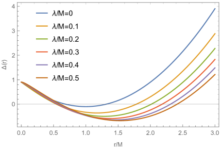
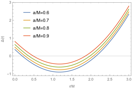
Figure 1: The horizon positions of rotating black holes with PFDM for different parameters, left panel: $a/M=0.95$, right panel: $\lambda/M=0.1$. The variations in the parameter $\lambda$ mainly affect the position of the outer horizon, while the rotation $a$ influences the position of both inner and outer horizons significantly.

III Dark matter influence on the superradiant amplification factor of massive scalar field

In this section, we consider the superradiance phenomenon of massive scalar field in a rotating black hole in the presence of PFDM. The equation of motion for a massive scalar field $\Phi$ is governed by the Klein-Gordon equation Bezerra:2013iha

$$\left(\nabla^{a}\nabla_{a}-\mu^{2}\right)\Phi=(\sqrt{-g})^{-1}\partial_{\mu}\left(\sqrt{-g}g^{\mu\nu}\partial_{\nu}\Phi\right)-\mu^{2}\Phi=0,$$ (17)

where $\mu$ is the mass of the scalar field. We can rewrite (17) more explicitly in the Boyer-Lindquist coordinates as

$$\left(-a^{2}\operatorname{sin}^{2}\theta+\frac{\left(a^{2}+r^{2}\right)^{2}}{\Delta}\right)\partial_{t}^{2}\Phi+\frac{2a\left(a^{2}+r^{2}-\Delta\right)}{\Delta}\partial_{t}\partial_{\phi}\Phi+\left(-\operatorname{csc}^{2}\theta+\frac{a^{2}}{\Delta}\right)\partial_{\phi}^{2}\Phi-\partial_{r}\left(\Delta\partial_{r}\Phi\right)-\frac{1}{\operatorname{sin}\theta}\partial_{\theta}\left(\operatorname{sin}\theta\partial_{\theta}\Phi\right)$$

$$+\mu^{2}\left(r^{2}+a^{2}\operatorname{cos}^{2}\theta\right)\Phi=0,$$ (18)

Since the background spacetime is stationary and axial-symmetric, we use following ansatz to separate the scalar perturbation Konoplya:2018arm ,

$$\Phi\left(x^{\mu}\right)=e^{-i\omega t}e^{im\phi}S_{lm}(\theta)R_{lm}(r),$$ (19)

Here, $S_{lm}(\theta)$ is spheroidal harmonics with $-m\leq l\leq m$ and $R_{lm}(r)$ is the radial part of the wave function. Substituting (19) to (18),Eq. (18) can be separated into

$$\frac{d}{dr}\left(\Delta\frac{d}{dr}R_{lm}(r)\right)+\left(\frac{\left((a^{2}+r^{2})\omega-am\right)^{2}}{\Delta}-(r^{2}\mu^{2}-2am\omega+a^{2}\omega^{2}+\Lambda_{lm})\right)R_{lm}(r)=0,$$ (20)

$$\frac{1}{\sin\theta}\frac{d}{d\theta}\left(\sin\theta\frac{dS_{lm}}{d\theta}\right)+\left(a^{2}\left(\omega^{2}-\mu^{2}\right)\cos^{2}\theta-\frac{m^{2}}{\sin^{2}\theta}+\Lambda_{lm}\right)S_{lm}(\theta)=0,$$ (21)

where $\Lambda_{lm}$ is the eigenvalues of the angular equation. In the non-rotating limit $a^{2}\omega^{2}\ll 1$, the eigenvalue $\Lambda_{lm}$ approaches $l(l+1)$ . The only interesting part is the Eq.(20). By changing variable $U(r)=\sqrt{a^{2}+r^{2}}R_{lm}$, and introduce the tortoise coordinate $dr_{*}=\frac{r^{2}+a^{2}}{\Delta}dr$ . Then, the radial function (20) takes the following Schrodinger-type equation

$$\frac{d^{2}U(r_{*})}{dr_{*}^{2}}+V(r)U(r_{*})=0,$$ (22)

with the effective potential $V(r)$ given by

$$V(r)= \left(\omega-\frac{am}{a^{2}+r^{2}}\right)^{2}-\frac{\Delta\left(l(l+1)+r^{2}\mu^{2}-2ma\omega+a^{2}\omega^{2}\right)}{\left(a^{2}+r^{2}\right)^{2}}$$

$$-\frac{\Delta^{2}}{\left(a^{2}+r^{2}\right)^{3}}+\frac{3r^{2}\Delta^{2}}{\left(a^{2}+r^{2}\right)^{4}}-\frac{\Delta\left(-2Mr+2r^{2}-\lambda r-\lambda r\ln\left(\frac{r}{\lambda}\right)\right)}{\left(a^{2}+r^{2}\right)^{4}}.$$ (23)

Before we proceed, we would like to mention the scattering of the scalar field under the effective potential. The asymptotic behaviors of the effective potential at the event horizon and spatial infinity are as follows

$$\lim_{r\rightarrow r_{h}}V(r)=\left(\omega-m\Omega_{h}\right)^{2}\equiv k_{h}^{2},\quad\Omega_{h}\equiv\frac{a}{r_{h}^{2}+a^{2}},$$ (24)

$$\lim_{r\rightarrow\infty}V(r)=\omega^{2}-\lim_{r\rightarrow\infty}\frac{r^{2}\mu^{2}\Delta}{(r^{2}+a^{2})^{2}}=\omega^{2}-\mu^{2}\equiv k_{\infty}^{2},$$ (25)

where $\Omega_{h}$ is the angular velocity of the event horizon.

Then, we have the following asymptotic behaviour of the solutions (boundary conditions) for Eq.(22)

$$U(r_{*})=Te^{-ik_{h}r_{*}},\quad r_{*}\rightarrow-\infty(r\rightarrow r_{h}),$$

$$U(r_{*})=Ie^{-ik_{\infty}r_{*}}+Re^{ik_{\infty}r_{*}},\quad r_{*}\rightarrow\infty(r\rightarrow\infty).$$ (26)

Thus the wave at horizon and asymptotic infinity becomes simple plane wave with different frequency. There is in-going wave at horizon with amplitude ${T}$, and at infinity, there are both in-going wave with an amplitude ${I}$ and a reflected outgoing wave with amplitude ${R}$. Now, by computing and equating the Wronskian quantity

$$W=(U\frac{dU^{*}}{dr_{*}}-U^{*}\frac{dU}{dR_{*}})$$ (27)

at the event horizon and spatial infinity we can get

$$\left|{R}\right|^{2}=\left|I\right|^{2}-\frac{\omega-m\Omega_{h}}{\sqrt{\omega^{2}-\mu^{2}}}\left|T\right|^{2}.$$ (28)

which implies that the amplitude of the reflected waves must be larger than the amplitude of the incident wave if the condition

$$\mu<\omega<m\Omega_{h},$$ (29)

is obeyed and therefore, the super-radiant scattering occurs ($|R|^{2}>|I|^{2}$) .

To access the magnitude of super-radiance, the amplification factor can be defined, which reads

$$Z_{lm}=\frac{|R|^{2}}{|I|^{2}}-1.$$ (30)

To concretely compute $Z_{lm}$ , we must solve radial equation (20). However, the radial equation (20) is not exactly solvable analytically, thus we will take advantage of a semi-analytical method which is called “analytical asymptotic matching” Starobinsky:1973aij . The procedure of this approach is that, we first find two approximate solutions each valid over a partial range and then match the two solutions in the overlapping region. After matching,a single approximate solution can be obtained. In this paper, we call these two regions “near-region” and “far-region” which respectively, denote the region around event horizon ($r-r_{h}\ll\omega^{-1}$) and far away from the event horizon ($r-r_{h}\gg M$). And the two solutions have to be in an “overlapping region” to match where $M\ll r-r_{h}\ll\omega^{-1}$.

By applying this method, we should introduce two assumptions: we should first take the low-frequency regime of the perturbation $a\omega\ll 1$ and we also assume BH’s size is smaller than the Compton wavelength of the scalar field $\Phi$ i.e., $M\omega\ll 1$ (or $\mu M\ll 1$) Detweiler:1980uk .

The radial equation (20) can be rewritten in the form

$$\Delta^{2}\frac{d^{2}R_{lm}(r)}{dr^{2}}+\Delta\frac{d\Delta}{dr}\frac{dR_{lm}(r)}{dr}+((\omega(a^{2}+r^{2})-am)^{2}-\Delta(r^{2}\mu^{2}-2am\omega+a^{2}\omega^{2}+l(l+1)))R_{lm}(r)=0,$$ (31)

In Kerr black hole, we know that $\Delta_{K}=r^{2}-2Mr+a^{2}=(r-r_{h})(r-r_{c})$.While in our PFDM case with two horizons, because of the log term, $\Delta$ in (31) can only be expressed as $\Delta=r^{2}-2Mr+a^{2}-\lambda r\ln({\frac{r}{\lambda}})=(r-r_{h})(r-r_{c})\sigma(r)$ where $\sigma(r)$ should be a monotonic function with no zeros. However, as plotted in Fig. 2, at least in our interested parameter region($\lambda$ region), we can observe that $\sigma(r)\approx 1$ from horizon to infinity , so in order to solve the Eq.(31) semi-analytically, we still approximate $\Delta$ as $(r-r_{h})(r-r_{c})$ in PFDM case without loss of much accuracy.Taking into account the correction caused by $\sigma(r)$ is interesting but difficult.It may need significant modification to the semi-analytical treatment of Teukolsky equation.But this correction is small compared to the shift of $r_{h}$ and $r_{c}$ caused by dark matter profile, so we only focus on the leading order correction caused by dark matter in this work.

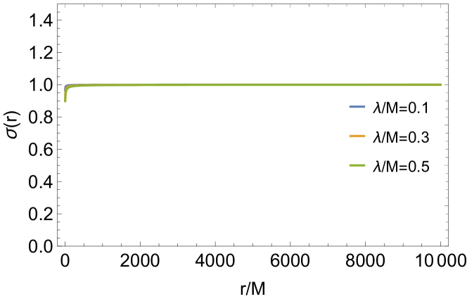
Figure 2: The numerical results of the proportional function $\sigma(r)$ with $a/M=0.95$ and $\lambda/M=0.1$, $\lambda/M=0.3$, $\lambda/M=0.5$.It can be seen that for all the range of $r$, $\sigma(r)$ approaches $1$ so we can approximate $\sigma$ to $1$ in the discussion.

By applying the change of variable $x=\frac{r-r_{h}}{r_{h}-r_{c}}$ and also using approximation $a\omega\ll 1$, the equation (31) can be rewritten as

$$x^{2}(1+x)^{2}\frac{d^{2}R_{lm}(x)}{dx^{2}}+x(x+1)(2x+1)\frac{dR_{lm}(x)}{dx}$$

$$+\left(k^{2}x^{4}-\left(\omega^{2}a^{2}+l(l+1)\right)x(x+1)-\mu^{2}\left(\left(r_{h}-r_{c}\right)x+{r}_{h}\right)^{2}x(x+1)+B^{2}\right)R_{lm}(x)=0,$$ (32)

where

$$x =\frac{r-{r}_{h}}{{r}_{h}-{r}_{c}},$$ (33)

$$k =\omega\left({r}_{h}-{r}_{c}\right),$$ (34)

$$B =\frac{{r}_{h}^{2}}{{r}_{h}-{r}_{c}}\left(\omega-m\Omega_{h}\right).$$ (35)

In the following, we will solve Eq.(32) in the near horizon limit and far-region limit and use asymptotic matching method to compute the reflection coefficient.

(i) Near-(horizon) region solution When approaching the event horizon, we have $kx\ll 1$ and $\mu^{2}((r_{h}-r_{c})x+r_{h})^{2}\approx\mu^{2}r_{h}^{2}\ll 1$, so equation (32) can be reduced to

$$x^{2}(x+1)^{2}\frac{d^{2}R_{lm}(x)}{dx^{2}}+x(x+1)(2x+1)\frac{dR_{lm}(x)}{dx}+\left(B^{2}-l(l+1)x(x+1)\right)R_{lm}(x)=0.$$ (36)

The general solution of equation (36) satisfying the boundary condition (26) is given by the hypergeometric functions

$$R_{lm}(x)=C\left(\frac{x+1}{x}\right)^{iB}\times\quad_{2}F_{1}(-l,l+1,1-2iB,-x),$$ (37)

where ${}_{2}F_{1}(-l,l+1,1-2iB,-x)$ is hypergeometric function. In order to match the solutions, it is essential to know that the large $x$ behavior of above solution is

$$R_{lm}(x) \sim Cx^{l}\frac{\Gamma(1-2iB)\Gamma(2l+1)}{\Gamma(1+l-2iB)\Gamma(l+1)}+Cx^{-l-1}\frac{\Gamma(1-2iB)\Gamma(-2l-1)}{\Gamma(-l)\Gamma(-l-2iB)}.$$ (38)

(ii) Far-region solution  In this region we consider $x\rightarrow\infty$, the equation (32) is approximately given by

$$\frac{d^{2}R_{lm}(x)}{dx^{2}}+\frac{2}{x}\frac{dR_{lm}(x)}{dx}+\left(D^{2}-\frac{l(l+1)}{x^{2}}\right)R_{lm}(x)=0,$$ (39)

where $D=(r_{h}-r_{c})\sqrt{\omega^{2}-\mu^{2}}$ . The general solution of equation (39) is

$$R_{lm}(x) =A_{1}\exp(-iDx)x^{l}U(l+1,2l+2,2iDx)+A_{2}\exp(-iDx)x^{-l-1}U(-l,-2l,2iDx),$$ (40)

where $U(l+1,2l+2,2iDx)$ and $U(-l,-2l,2iDx)$ are confluent hyper-geometric functions. To match the solution above with (38), it is essential to know the small $x$ behavior of the above solution Brito:2015oca

$$R_{lm}(x)\sim A_{1}x^{l}+A_{2}x^{-l-1}.$$ (41)

(iii) Solution in the overlapping region  Now, the two asymptotic solutions Eq.(38) and Eq.(41) can be matched since they have an overlapping region. At first step, we can get the following coefficient relations,

$$A_{1} =C\frac{\Gamma(1-2iB)\Gamma(2l+1)}{\Gamma(l+1)\Gamma(l+1-2iB)},$$

$$A_{2} =C\frac{\Gamma(1-2iB)\Gamma(-1-2l)}{\Gamma(-l-2iB)\Gamma(-l)}.$$ (42)

And we know the solution (26) takes the following form when $r\rightarrow\infty$,

$$R_{lm}\sim\frac{U_{\infty}\left(r_{*}\right)}{r}\sim{I}\frac{\exp\left(-ik_{\infty}r_{*}\right)}{r}+{R}\frac{\exp\left(ik_{\infty}r_{*}\right)}{r}.$$ (43)

Then, we need to connect the coefficients $A_{1}$ and $A_{2}$ with the coefficients $I$ and $R$ in the asymptotic solution (26). In order to do that, we expand (40) at infinity and match with (43). After some algebra, we obtain the analytical expression for $I$ and $R$

$${I}=A_{1}\frac{(-2i)^{-l-1}D^{-l}\Gamma(2l+2)}{k_{\infty}\Gamma(l+1)}+A_{2}\frac{(-2i)^{l}D^{l+1}\Gamma(-2l)}{k_{\infty}\Gamma(-l)},$$

$${R}=A_{1}\frac{(2i)^{-l-1}D^{-l}\Gamma(2l+2)}{k_{\infty}\Gamma(l+1)}+A_{2}\frac{(2i)^{l}D^{l+1}\Gamma(-2l)}{k_{\infty}\Gamma(-l)}.$$ (44)

Thus we can get the amplification factor for scalar wave (30) as follows

$$Z_{lm}(\omega)=-4BD^{2l+1}\frac{(l!)^{4}}{((2l)!)^{2}((2l+1)!!)^{2}}\times\prod_{k=1}^{l}\left(1+\frac{4B^{2}}{k^{2}}\right).$$ (45)

There will be superradiant phenomena when $Z_{lm}>0$ . In Fig. 3, we plot $Z_{11}$ for different angular momentum $a$ and PFDM parameter $\lambda$ .

From the left panel, we observe that the super-radiant amplification factor monotonically increases with the black hole angular momentum $a$. This indicates that the superradiant effect becomes more pronounced as the black hole rotates faster. In the right panel, roughly speaking, the superradiant amplification weakens gradually as the dark matter parameter increases.

Interestingly, from the right panel of Fig. 3, there is an intersection between the amplification factor of the Kerr black hole($\lambda/M=0$) and that of the PFDM rotating black hole. It means that in some frequency domain, as the dark matter density $\lambda$ increases, the super-radiance will first enhance and then decrease thus has the non-monotonous behavior. To certify this point more, we plot the peak amplification factor within the parameter range $\lambda/M=0$ to $\lambda/M=0.1$ in Fig. 4. From Fig. 4, we notice that as the amount of dark matter increases in the region between $0<\frac{\lambda}{M}<0.1$, the peak amplification factor initially increases and then gradually decreases. We do not have a direct physical understanding of this phenomenon up to now. It would be interesting to further investigate whether this behavior can be understood by considering correction caused by $\sigma(r)$ or there is some physical reason behind.

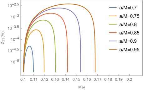
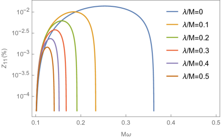
Figure 3: The amplification factor $Z_{11}$ for $l=m=1,\mu M=0.1$. We set parameters $\lambda/M=0.3$ in left panel, parameters $a/M=0.95$ in right panel. The left panel shows that the superradiant amplification increases monotonically with the black hole spin $a$. The right panel shows that the superradiant amplification effect decreases as the dark matter parameter $\lambda$ increases. Different plot lines in two figures have different frequency ranges, which are limited by the superradiance condition $\mu<\omega<m\Omega_{h}$.

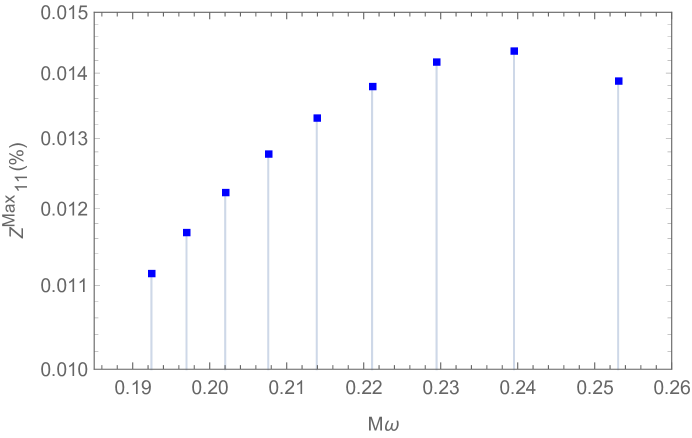
Figure 4: The peak amplification factor $Z^{Max}_{11}$ for $l=m=1,\mu M=0.1$. The squares in the figure represent dark matter parameters ranging from$\lambda/M=0$ to $\lambda/M=0.1$, from right to left. The figure depicts the trend of the peak amplification factor increasing and then decreasing with the increase in the PFDM parameter.

IV Energy extraction from black hole

In last section, we have demonstrated the effect of dark matter density $\lambda$ on the super-radiant amplification factor of scalar waves. While the amplification factor is the most direct quantity to characterize the strength of super-radiance, it is not so straightforward to observe. So in this section, in order to show the effect of dark matter on super-radiance more intuitively, we will investigate other physical quantity which is directly related to super-radiance. It has long been known that super-radiance can be used to extract energy from black hole. Thus in this section, we will further investigate the energy extraction behavior and find the effect of PFDM parameters on the net extracted energy from black hole.

Firstly, the outgoing energy $\dot{E}_{out}$ measured by an observer at infinity can be obtained by calculating the energy-momentum tensor of the field. For a monochromatic scalar field, the outgoing energy flux is as follows Brito:2015oca ; Wondrak:2018fza ,

$$\dot{E}_{out}=\frac{\omega k_{\infty}}{2}|R|^{2}.$$ (46)

we leave the derivation of this expression to Appendix A. In this section, we use the massless scalar waves($\mu=0$) to extract energy without loss of generality. The generalization to massive scalar waves will be straightforward.

It is easy to generalize this to non-monochrome case. In non-monochrome case, we need to integrate the flux contribution of each mode and take into account the Bose-Einstein distribution since we focus on scalar wave. Thus the total extracted energy becomes

$$\dot{E}_{tot}=\int\mathrm{d^{3}k}\frac{\omega k_{\infty}}{2}|R|^{2}n(\omega)=\int d\omega\frac{\omega k_{\infty}}{2}|R|^{2}\omega^{2}n(\omega).$$ (47)

Here, $n(\omega)$ represents the (normalized) distribution function

$$n(\omega)=\frac{1}{8\pi\zeta(3)T_{tem}^{3}\left(\exp\left[\omega/T_{tem}\right]-1\right)},$$ (48)

where $8\pi\zeta(3)T_{tem}^{3}$ is the normalization factor, $\zeta(x)$ is the Riemann zeta function with $\zeta(3)\approx 1.2$. $T_{tem}$ is the temperature of radiation. As $|R|^{2}$ in Eq.(47) does not depend on $T_{tem}$, the choice of temperature $T_{tem}$ will not affect the result qualitatively but only shift the specific value of extracted energy. However,physically, we should choose $T_{tem}\gg T_{H}$ to ignore the contribution of Hawking radiation.

By taking into account the energy of in-going waves, we can obtain the incident energy flux using the same method as obtaining (46). By subtracting the energy of in-going waves, we can determine the net energy extracted from the black hole via super-radiance as follows

$$\dot{E}_{\text{ptot}}=\int\mathrm{d^{3}k}\frac{\omega k_{\infty}}{2}\left(|R|^{2}-|I|^{2}\right)n(\omega)=\int d\omega\frac{\omega k_{\infty}}{2}(|R|^{2}-|I|^{2})\omega^{2}n(\omega).$$ (49)

Fig. 5 plots the relation between net extracted energy profile (the integrand in Eq.(49))and wave frequency. Total net extracted energy is the area of the region between the curve and x-axis. Combining with the data presented in Table 1, it can be observed that the net energy extraction from PFDM rotating black holes via super-radiance is smaller than that from Kerr black holes , and it decreases further with increasing the dark matter density. From Table 1, we can also observe that as the PFDM parameter increases, the corresponding ergo-sphere shrinks. This gives the reason why the extracted energy decrease as dark matter density $\lambda$ increases from the perspective of black hole structure.

Figure 5: The net extracted energy profile $\dot{E}_{itgp}$ at infinity for $l=m=1$ . The spin $a$ are set to $0.95M$. As seen from this panel, the net extracted energy decreases with increasing dark matter density and is smaller for dark matter black hole compared to Kerr black holes.We choose $T_{tem}=2.7K$ for this plot

$\lambda/M$	Infinite redshift surface	horizon($r_{h}$)	Ergo-sphere	Ratio	$\dot{E}_{p11}$
0	2	1.31225	0.68775	1.5241	$6.76136\times 10^{-5}$
0.1	2.31416	1.78136	0.532802	1.2991	$1.27471\times 10^{-5}$
0.3	2.65401	2.18148	0.472529	1.21661	$6.70288\times 10^{-6}$
0.5	2.87452	2.41299	0.461526	1.19127	$4.63462\times 10^{-6}$

Table 1: Under the condition $a/M=0.95$, the infinite redshift surface, event horizon, ergosphere and ratios corresponding to different parameters $\lambda$, as well as the net energy extraction in the $l=m=1$ mode. The difference between the infinite redshift surface radius and the event horizon radius represents the ergosphere range, while their ratio indicates the relative variation of the ergosphere. The table reflects that both the area of ergosphere and the pure energy extraction decrease as the dark matter parameter increases.

V superradiant instability analysis

It has long been known that superradiance can trigger the instability of black hole spacetime Witek:2012tr . So there is a natural question about whether this instability can be affected by the presence of dark matter. In this section, we will explore the influence of dark matter parameters on the stability of black holes using the black hole bomb model  Press:1972zz .

The black hole bomb model puts a mirror outside the black hole to confine and amplify waves through continuous reflections. The presence of mirror is equivalent to impose an effective potential well outside the black hole which is essential to trigger the super-radiant instability.

From equation (31) we have

$$\Delta\frac{d}{dr}\left(\Delta\frac{dR_{lm}(r)}{dr}\right)+\alpha R_{lm}(r)=0,$$ (50)

where

$$\alpha=(\omega(a^{2}+r^{2})-am)^{2}-\Delta(r^{2}\mu^{2}-2am\omega+a^{2}\omega^{2}+l(l+1)).$$ (51)

According to the black hole bomb mechanism, the solution of the radial equation (50) takes the following form

$$R_{lm}\sim\begin{cases}e^{-i(\omega-m\Omega_{h})r_{*}}&\text{ as }r\rightarrow r_{h}\left(r_{*}\rightarrow-\infty\right)\\ \frac{e^{-\sqrt{\mu^{2}-\omega^{2}r_{*}}}}{r}&\text{ as }r\rightarrow\infty\left(r_{*}\rightarrow\infty\right)\end{cases}$$ (52)

From the equation above, we can deduce the boundary conditions: at the black hole horizon, there exists only a purely ingoing wave, while under the condition $\omega^{2}<\mu^{2}$, at spatial infinity, there exists a decaying scalar wave.

Now, with the new radial function

$$\psi_{lm}\equiv\sqrt{\Delta}R_{lm},$$ (53)

the equation (50) becomes

$$(\frac{d^{2}}{d^{2}r}+\omega^{2}-V_{eff})\psi_{lm}=0,$$ (54)

where

$$\omega^{2}-V_{eff}=\frac{\alpha+\beta}{\Delta^{2}},$$ (55)

$$\beta=\frac{\left(2M-2r+\lambda+\lambda\ln\left(\frac{r}{\lambda}\right)\right)^{2}}{4}-\frac{\left(2-\frac{\lambda}{r}\right)\left(a^{2}-2Mr+r^{2}-r\lambda\ln\left(\frac{r}{\lambda}\right)\right)}{2}.$$

By discarding the terms $\mathscr{O}(1/r^{2})$, the effective potential can be approximated as follows

$$V_{a}=\mu^{2}+\frac{\left(\mu^{2}-2\omega^{2}\right)\left(2M+\lambda\ln\left(\frac{r}{\lambda}\right)\right)}{r}.$$ (56)

If the derivative of the effective potential is asymptotically positive, then there will exist a potential well that can confine the super-radiant waves and trigger instability. By taking the derivative, we can get the derivative form of equation (56) as follows

$$V_{a}^{\prime}=\frac{\left(2\omega^{2}-\mu^{2}\right)\left(2M-\lambda(1-\ln\left(\frac{r}{\lambda}\right))\right)}{r^{2}}.$$ (57)

By demanding $2M-\lambda(1-\ln\frac{r}{\lambda})>0$, or equivalently $r>\lambda e^{1-\frac{2M}{\lambda}}$. To satisfy condition $V_{a}^{\prime}>0$, we need to let

$$2\omega^{2}-\mu^{2}>0$$ (58)

and then we can obtain

$$\mu<\sqrt{2}\omega$$ (59)

Combining condition $\omega<m\Omega_{h}$, we can deduce

$$\mu<\sqrt{2}m\Omega_{h}.$$ (60)

From the above equation, we see that compared to Kerr black hole, the presence of dark matter has no influence on the superradiant instability condition of the black hole.

VI conclusion and disscuion

In this work, we investigated the super-radiant amplification effect of rotating black hole surrounded by dark matter.We consider the scattering of the massive scalar field to show this. Despite some non-monotonous behaviors for small $\lambda$, generally speaking, we found that as the dark matter parameter increases, the super-radiant amplification factor decreases which means the presence of dark matter will suppress the super-radiance. We computed the energy extraction behavior to further support our results and showed that the reason for this suppression is due to shrink of the ergo-sphere. Finally, we discussed the instability caused by superradiance within the context of the black hole bomb mechanism.We found that the presence of dark matter does not change the mass condition for black hole superradiant instability.

For future research, we will firstly try to find a clear explanation about the non-monotonous behavior we found in Fig.3.The other direction will be to consider the super-radiant behavior of black hole solution in the presence of quintessential dark energy profile such as Kiselev black hole Kiselev:2002dx and investigated the effect of dark energy on the black hole super-radiance. Finally, as the black hole super-radiance has huge potential to be detected in the future,it is interesting to see if the superradiant properties we found in this paper can be used to search the dark matter in universe.

Appendix A Details for the derivation of (46)

In this appendix, we give the detailed derivation of (46). The Lagrangian density $\mathscr{L}$ of a complex scalar field is

$$\mathscr{L}=\frac{1}{2}g^{\mu\nu}\partial_{(\mu}\Phi^{*}\partial_{\nu)}\Phi-\frac{1}{2}\mu^{2}|\Phi|^{2},$$ (61)

where $\partial_{(\mu}\Phi^{*}\partial_{\nu)}\Phi=\frac{1}{2}\left(\partial_{\mu}\Phi^{*}\partial_{\nu}\Phi+\partial_{\nu}\Phi^{*}\partial_{\mu}\Phi\right)$. The total energy fluxes at infinity per unit solid angle is given by Brito:2015oca

$$\frac{d^{2}E}{dtd\Omega}=\lim_{r\rightarrow+\infty}r^{2}T_{t}^{r},$$ (62)

where $T^{\mu}_{\nu}$ is the symmetric stress-energy tensor

$$T_{\nu}^{\mu}=g^{\mu\lambda}\partial_{(\lambda}\Phi^{*}\partial_{\nu)}\Phi-\delta_{\nu}^{\mu}\mathscr{L}.$$ (63)

From the previous context, we know that the scalar field is

$$\Phi\left(x^{\mu}\right)=e^{-i\omega t}e^{im\phi}S_{lm}(\theta)R_{lm}(r),$$ (64)

and the asymptotic solution at the infinity is

$$R_{lm}(r)=\frac{Ie^{-ik_{\infty}r}+Re^{ik_{\infty}r}}{r}.$$ (65)

Now, when we substitute (61), (64), and $g^{\mu\nu}$ into (63), we can get $T_{t}^{r}$ as follows

$$T_{t}^{r}=\frac{1}{2}g^{rt}(\partial_{t}\Phi^{*}\partial_{t}\Phi+\partial_{t}\Phi^{*}\partial_{t}\Phi)+\frac{1}{2}g^{rr}(\partial_{r}\Phi^{*}\partial_{t}\Phi+\partial_{t}\Phi^{*}\partial_{r}\Phi)$$

$$+\frac{1}{2}g^{r\theta}(\partial_{\theta}\Phi^{*}\partial_{t}\Phi+\partial_{t}\Phi^{*}\partial_{\theta}\Phi)+\frac{1}{2}g^{r\phi}(\partial_{\phi}\Phi^{*}\partial_{t}\Phi+\partial_{t}\Phi^{*}\partial_{\phi}\Phi).$$ (66)

Here, as we have deduced from the metric $g^{\mu\nu}$ that $g^{rt}$, $g^{r\theta}$, and $g^{r\phi}$ are all equal to zero, we can remove the corresponding three terms, thus ultimately obtaining the following form,

$$T_{t}^{r}=\frac{1}{2}g^{rt}(\partial_{t}\Phi^{*}\partial_{t}\Phi+\partial_{t}\Phi^{*}\partial_{t}\Phi).$$ (67)

We substitute (65) into the above equation and can obtain:

$$T_{t}^{r}=\frac{1}{2}g^{rr}(-i\omega e^{i\omega t}e^{-im\phi}S^{*}_{lm}(\theta)R^{*^{\prime}}_{lm}(r)e^{-i\omega t}e^{im\phi}S_{lm}(\theta)R_{lm}(r)$$

$$+i\omega e^{i\omega t}e^{-im\phi}S^{*}_{lm}(\theta)R^{*}_{lm}(r)e^{-i\omega t}e^{im\phi}S_{lm}(\theta)R^{{}^{\prime}}_{lm}(r)).$$ (68)

The terms $R^{*^{\prime}}_{lm}(r)$ and $R^{{}^{\prime}}_{lm}(r)$ denote the derivative with respect to $r$. Then we substitute (65) into (68) and after some calculations and simplification, we can obtain

$$\frac{dE_{out}}{dt}=\frac{\omega k_{\infty}}{2}|R|^{2}.$$ (69)

References

- (1) B. P. Abbott et al. (LIGO Scientific and Virgo), Observation of Gravitational Waves from a Binary Black Hole Merger, Phys. Rev. Lett. 116, no.6, 061102 (2016)
- (2) B. P. Abbott et al. (LIGO Scientific and Virgo), Tests of General Relativity with the Binary Black Hole Signals from the LIGO-Virgo Catalog GWTC-1, Phys. Rev. D. 100, no.10, 104036 (2019)
- (3) K. Akiyama et al. (Event Horizon Telescope), First M87 Event Horizon Telescope Results. IV. Imaging the Central Supermassive Black Hole, Astrophys. J. Lett. 875, no.1, L4 (2019)
- (4) K. Akiyama et al. (Event Horizon Telescope), First M87 Event Horizon Telescope Results. I. The Shadow of the Supermassive Black Hole, Astrophys. J. Lett. 875, L1 (2019)
- (5) K. Akiyama et al. (Event Horizon Telescope), First Sagittarius A* Event Horizon Telescope Results. I. The Shadow of the Supermassive Black Hole in the Center of the Milky Way, Astrophys. J. Lett. 930, no.2, L12 (2022)
- (6) K. Akiyama et al. (Event Horizon Telescope), First Sagittarius A* Event Horizon Telescope Results. III. Imaging of the Galactic Center Supermassive Black Hole, Astrophys. J. Lett. 930, no.2, L14 (2022)
- (7) R. Penrose, Gravitational collapse: The role of general relativity, Riv. Nuovo Cim. 1, 252-276 (1969)
- (8) R. Penrose and R. M. Floyd, Extraction of rotational energy from a black hole, Nature 229, 177-179 (1971)
- (9) C. W. Misner, Interpretation of gravitational-wave observations, Phys. Rev. Lett. 28, 994-997(1972)
- (10) R. Brito, V. Cardoso and P. Pani, Superradiance: New Frontiers in Black Hole Physics, Lect. Notes Phys. 906, pp.1-237 (2015) 2020,
- (11) S. A. Teukolsky, Perturbations of a rotating black hole. 1. Fundamental equations for gravitational electromagnetic and neutrino field perturbations, Astrophys. J. 185, 635-647 (1973)
- (12) M. Richartz and A. Saa, Superradiance without event horizons in General Relativity, Phys. Rev. D 88, 044008 (2013)
- (13) V. Cardoso, R. Brito and J. L. Rosa, Superradiance in stars, Phys. Rev. D 91, no.12, 124026 (2015)
- (14) K. Glampedakis, S. J. Kapadia and D. Kennefick, Superradiance-tidal friction correspondence, Phys. Rev. D 89, no.2, 024007 (2014)
- (15) H. Witek, V. Cardoso, A. Ishibashi and U. Sperhake, Superradiant instabilities in astrophysical systems, Phys. Rev. D 87, no.4, 043513 (2013)
- (16) H. Furuhashi and Y. Nambu, Instability of massive scalar fields in Kerr-Newman space-time, Prog. Theor. Phys. 112, 983-995 (2004)
- (17) V. Cardoso, O. J. C. Dias and S. Yoshida, Classical instability of Kerr-AdS black holes and the issue of final state, Phys. Rev. D 74, 044008 (2006)
- (18) S. R. Dolan, Instability of the massive Klein-Gordon field on the Kerr spacetime, Phys. Rev. D 76, 084001 (2007)
- (19) S. Hod, On the instability regime of the rotating Kerr spacetime to massive scalar perturbations, Phys. Lett. B 708, 320-323 (2012)
- (20) S. R. Dolan, Superradiant instabilities of rotating black holes in the time domain, Phys. Rev. D 87, no.12, 124026 (2013)
- (21) Z. Zhu, S. J. Zhang, C. E. Pellicer, B. Wang and E. Abdalla, Stability of Reissner-Nordström black hole in de Sitter background under charged scalar perturbation, Phys. Rev. D 90, no.4, 044042 (2014)
- (22) S. R. Green, S. Hollands, A. Ishibashi and R. M. Wald, Superradiant instabilities of asymptotically anti-de Sitter black holes, Class. Quant. Grav. 33, no.12, 125022 (2016)
- (23) Y. Huang, D. J. Liu, X. h. Zhai and X. z. Li, Instability for massive scalar fields in Kerr-Newman spacetime, Phys. Rev. D 98, no.2, 025021 (2018)
- (24) K. Destounis, Superradiant instability of charged scalar fields in higher-dimensional Reissner-Nordström-de Sitter black holes, Phys. Rev. D 100, no.4, 044054 (2019)
- (25) J. H. Huang, W. X. Chen, Z. Y. Huang and Z. F. Mai, Superradiant stability of the Kerr black holes, Phys. Lett. B 798, 135026 (2019)
- (26) R. Li, Y. Zhao, T. Zi and X. Chen, Superradiance and dynamical evolution of a charged scalar field in an asymptotically anti–de-Sitter dilatonic black hole, Phys. Rev. D 99, no.8, 084045 (2019)
- (27) J. H. Xu, Z. H. Zheng, M. J. Luo and J. H. Huang, Analytic study of superradiant stability of Kerr–Newman black holes under charged massive scalar perturbation, Eur. Phys. J. C 81, no.5, 402 (2021)
- (28) H. S. Vieira, V. B. Bezerra and C. R. Muniz, Instability of the charged massive scalar field on the Kerr–Newman black hole spacetime, Eur. Phys. J. C 82, no.10, 932 (2022)
- (29) W. H. Press and S. A. Teukolsky, Floating Orbits, Superradiant Scattering and the Black-hole Bomb, Nature 238, 211-212 (1972)
- (30) V. Cardoso, O. J. C. Dias, J. P. S. Lemos and S. Yoshida, The Black hole bomb and superradiant instabilities, Phys. Rev. D 70, 044039 (2004)
- (31) V. Cardoso, Black hole bombs and explosions: from astrophysics to particle physics, Gen. Rel. Grav. 45, 2079-2097 (2013)
- (32) C. A. R. Herdeiro, J. C. Degollado and H. F. Rúnarsson, Rapid growth of superradiant instabilities for charged black holes in a cavity, Phys. Rev. D 88, 063003 (2013)
- (33) S. R. Dolan, S. Ponglertsakul and E. Winstanley, Stability of black holes in Einstein-charged scalar field theory in a cavity, Phys. Rev. D 92, no.12, 124047 (2015)
- (34) O. J. C. Dias and R. Masachs, Charged black hole bombs in a Minkowski cavity, Class. Quant. Grav. 35, no.18, 184001 (2018)
- (35) C. Herdeiro, E. Radu and H. Rúnarsson, Kerr black holes with Proca hair, Class. Quant. Grav. 33, no.15, 154001 (2016)
- (36) C. A. R. Herdeiro and E. Radu, Dynamical Formation of Kerr Black Holes with Synchronized Hair: An Analytic Model, Phys. Rev. Lett. 119, no.26, 261101 (2017)
- (37) J. C. Degollado, C. A. R. Herdeiro and E. Radu, Effective stability against superradiance of Kerr black holes with synchronised hair, Phys. Lett. B 781, 651-655 (2018)
- (38) C. A. R. Herdeiro and E. Radu, Spherical electro-vacuum black holes with resonant, scalar -hair, Eur. Phys. J. C 80, no.5, 390 (2020)
- (39) A. Rahmani, M. Khodadi, M. Honardoost and H. R. Sepangi, Instability and no-hair paradigm in d-dimensional charged-AdS black holes, Nucl. Phys. B 960, 115185 (2020)
- (40) R. Brito, V. Cardoso and P. Pani, Black holes as particle detectors: evolution of superradiant instabilities, Class. Quant. Grav. 32, no.13, 134001 (2015)
- (41) V. C. Rubin, N. Thonnard and W. K. Ford, Jr., Rotational properties of 21 SC galaxies with a large range of luminosities and radii, from NGC 4605 /R = 4kpc/ to UGC 2885 /R = 122 kpc/, Astrophys. J. 238, 471 (1980)
- (42) M. Persic, P. Salucci and F. Stel, The Universal rotation curve of spiral galaxies: 1. The Dark matter connection, Mon. Not. Roy. Astron. Soc. 281, 27 (1996)
- (43) G. Bertone and D. Hooper, History of dark matter, Rev. Mod. Phys. 90, no.4, 045002 (2018)
- (44) V. V. Kiselev, Quintessence and black holes, Class. Quant. Grav. 20, 1187-1198 (2003).
- (45) M. H. Li and K. C. Yang, Galactic Dark Matter in the Phantom Field, Phys. Rev. D 86, 123015 (2012).
- (46) B. Toshmatov, Z. Stuchlík and B. Ahmedov, Rotating black hole solutions with quintessential energy, Eur. Phys. J. Plus 132, no.2, 98 (2017).
- (47) Z. Xu, J. Wang and X. Hou, Kerr–anti-de Sitter/de Sitter black hole in perfect fluid dark matter background, Class. Quant. Grav. 35, no.11, 115003 (2018).
- (48) A. Das, A. Saha and S. Gangopadhyay, Investigation of circular geodesics in a rotating charged black hole in the presence of perfect fluid dark matter, Class. Quant. Grav. 38, no.6, 065015 (2021)
- (49) X. Liang, Y. P. Hu, C. H. Wu and Y. S. An, Thermodynamics and evaporation of perfect fluid dark matter black hole in phantom background, arXiv:2308.00308 [gr-qc].
- (50) V. B. Bezerra, H. S. Vieira and A. A. Costa, The Klein-Gordon equation in the spacetime of a charged and rotating black hole, Class. Quant. Grav. 31, no.4, 045003 (2014)
- (51) R. A. Konoplya, Z. Stuchlík and A. Zhidenko, Axisymmetric black holes allowing for separation of variables in the Klein-Gordon and Hamilton-Jacobi equations, Phys. Rev. D 97, no.8, 084044 (2018)
- (52) A. A. Starobinsky, Amplification of waves reflected from a rotating ”black hole”., Sov. Phys. JETP 37, no.1, 28-32 (1973)
- (53) S. L. Detweiler, KLEIN-GORDON EQUATION AND ROTATING BLACK HOLES, Phys. Rev. D 22, 2323-2326 (1980)
- (54) M. F. Wondrak, P. Nicolini and J. W. Moffat, Superradiance in Modified Gravity (MOG), JCAP 12, 021 (2018)