Federated Representation Learning in the Under-Parameterized Regime

Abstract

Federated representation learning (FRL) is a popular personalized federated learning (FL) framework where clients work together to train a common representation while retaining their personalized heads. Existing studies, however, largely focus on the over-parameterized regime. In this paper, we make the initial efforts to investigate FRL in the under-parameterized regime, where the FL model is insufficient to express the variations in all ground-truth models. We propose a novel FRL algorithm FLUTE, and theoretically characterize its sample complexity and convergence rate for linear models in the under-parameterized regime. To the best of our knowledge, this is the first FRL algorithm with provable performance guarantees in this regime. FLUTE features a data-independent random initialization and a carefully designed objective function that aids the distillation of subspace spanned by the global optimal representation from the misaligned local representations. On the technical side, we bridge low-rank matrix approximation techniques with the FL analysis, which may be of broad interest. We also extend FLUTE beyond linear representations. Experimental results demonstrate that FLUTE outperforms state-of-the-art FRL solutions in both synthetic and real-world tasks.

1 Introduction

In the development of machine learning (ML), the role of representation learning has become increasingly essential. It transforms raw data into meaningful features, reveals hidden patterns and insights in data, and facilitates efficient learning of various ML tasks such as meta-learning (Tripuraneni et al., 2021), multi-task learning (Wang et al., 2016a), and few-shot learning (Du et al., 2020).

Recently, representation learning has been introduced to the federated learning (FL) framework to cope with the heterogeneous local datasets at participating clients (Liang et al., 2020). In the FL setting, it often assumes that all clients share a common representation, which works in conjunction with personalized local heads to realize personalized prediction while harnessing the collective training power (Arivazhagan et al., 2019; Collins et al., 2021; Zhong et al., 2022; Shen et al., 2023).

Existing theoretical analysis of representation learning usually assumes the adopted model is over-parameterized to almost fit the ground-truth model (Tripuraneni et al., 2021; Wang et al., 2016a). While this may be valid for expressive models like Deep Neural Networks (He et al., 2016; Liu et al., 2017) or Large Language Models (OpenAI, 2023; Touvron et al., 2023), it may be too restrictive for FL on resource-constrained devices, as adopting over-parameterized models in such a framework faces several significant challenges, as elaborated below.

• Computation limitation. In FL, edge devices like smartphones and Internet of Things (IoT) devices often have limited memory and lack computational power, which are not capable of either storing or training over-parameterized models (Wang et al., 2019; He et al., 2020; Kairouz et al., 2021).

• Communication overhead. In FL, the clients need to communicate updated model information with the server frequently. It thus becomes prohibitive to transmit a huge number of model updates for devices operating with limited communication energy and bandwidth.

• Privacy concern. Existing works show that excessively expressive models may “memorize” relevant information from local datasets, increasing the model’s susceptibility to reconstruction attacks  (Hitaj et al., 2017; Melis et al., 2019; Wang et al., 2018; Li et al., 2020) or membership inference (Tan et al., 2022).

Motivated by those concerns, in this work, we focus on federated representation learning (FRL) in the under-parameterized regime, where the parameterized model class is not rich enough to realize the ground-truth models across all clients. This is arguably a more realistic setting for edge devices supporting FL. Meanwhile, due to the inherent limitation of the expressiveness of the under-parameterized models, the algorithm design and theoretical guarantees in the over-parameterized regime do not naturally translate to this setting. We summarize our main contributions as follows.

• Algorithm design. A major challenge for FRL in the under-parameterized regime is the fact that the locally optimal representation may not be globally optimal. As a result, simply averaging the local representations may not converge to the global optimal solution. To cope with this challenge, we propose FLUTE, a novel FRL framework tailored for the under-parameterized setting. To the best of our knowledge, this is the first FRL framework that focuses on the under-parameterized regime. Our algorithm design features two primary innovations. First, we develop a new regularization term that generalizes the existing formulations in a non-trivial way. In particular, this new regularization term is designed to provably enhance the performance of FRL in the under-parameterized setting. Second, our algorithm contains a new and critical step of server-side updating by simultaneously optimizing both the representation layer and all local head layers. This represents a significant departure from existing approaches in FRL, particularly in over-parameterized settings where local heads are optimized solely on the client side. By leveraging information across these local heads, our approach could learn the ground-truth model more effectively.

• Theoretical guarantees. In terms of theoretical performance, we specialize FLUTE to the linear setting and analyze the sample complexity required for FLUTE to recover a near-optimal model, as well as characterizing its convergence rate. FLUTE achieves a sample complexity that scales in $\tilde{\mathcal{O}}\left(\frac{\max\{d,M\}}{M\epsilon^{2}}\right)$ for recovering an $\epsilon$-optimal model, where $d$ is the dimension of the input data and $M$ is the number of clients. This result indicates a linear sample complexity speedup in terms of $M$ in the high dimensional setting (i.e., $d\geq M$) compared with its single-agent counterpart (Hsu et al., 2012). Besides, it outperforms the sample complexity in the noiseless over-parameterized FRL setting (Collins et al., 2021) in terms of both $M$ and $d$. Moreover, we show that FLUTE converges to the optimal model exponentially fast when the number of samples is sufficiently large.

• Technical contributions. In the under-parameterized regime, we must analyze the convergence of both the representation and personalized heads toward their optimal estimations. This is in sharp contrast to the over-parameterized regime, where we only need to study the convergence of the representation column space to the ground truth (Collins et al., 2021; Zhong et al., 2022). Towards this end, we adopt a low-rank matrix approximation framework (Chen et al., 2023) of the ground-truth model. However, in contrast to conventional low-rank matrix approximation, in FRL, the global model is not accessible a priori but must be learned from distributed local datasets. Thus, the technical analysis needs to bound the unavoidable gradient discrepancy in the under-parameterized regime, as well as ensure that neither gradient discrepancy nor noise-induced errors accumulate over iterations. To address these technical challenges, we first provide new concentration results to ensure that the norm of the gradient discrepancy can be bounded when local datasets are sufficiently large. We then develop iteration-dependent upper bounds for sample complexity, which guarantee that the improvement in the estimation, i.e., the ’distance’ between our estimated model and the optimal low-rank model, can mitigate potential disturbances caused by gradient discrepancy and noise.

• Empirical evaluation. We conduct a series of experiments utilizing both synthetic datasets for linear FLUTE and real-world datasets, specifically CIFAR-10 and CIFAR-100 (Krizhevsky et al., 2009), for general FLUTE. The empirical results demonstrate the advantages of FLUTE, as evidenced by its superior performance over baselines, particularly in the scenarios where the level of under-parameterization is significant.

2 Related Work

Representation learning. Representation learning focuses on acquiring a representation across diverse tasks to effectively extract feature information (LeCun et al., 2015; Tripuraneni et al., 2021; Wang et al., 2016a; Finn et al., 2017). In the linear multi-task learning setting, Du et al. (2020) characterize the optimal solution of the empirical risk minimization (ERM) problem, demonstrating that the gap between the solution and the ground-truth representation is upper bounded by ${\mathcal{O}}\big{(}\sqrt{\frac{M+d}{MN}}\big{)}$, where $d$ is the dimension of data, $M$ is the number of clients and $N$ is the number of samples per task. Tripuraneni et al. (2021) give an upper bound $\mathcal{O}\big{(}\sqrt{\frac{d}{MN}}\big{)}$ using the Method-of-Moment estimator. Thekumparampil et al. (2021) also show the $\mathcal{O}\big{(}\sqrt{\frac{d}{MN}}\big{)}$ upper bound in their work. Duchi et al. (2022) consider data-dependent noise and show that the sample complexity required to recover the shared subspace of the linear models scales in $O\big{(}\log^{3}(Nd)\sqrt{\frac{d}{MN}}\big{)}$. These works, however, only focus on the over-parameterized regime in a centralized setting.

Federated representation learning. Recently, representation learning has been introduced to FL (Arivazhagan et al., 2019; Liang et al., 2020; Collins et al., 2021; Yu et al., 2020). Liang et al. (2020) propose an FRL framework named Fed-LG, where the distinct representations are stored locally and the common prediction head is forwarded to the server for aggregation. In contrast, Arivazhagan et al. (2019) propose FedPer, where a common representation is shared among clients, with personalized local heads kept at the client side. A similar setting is adopted by FedRep (Collins et al., 2021), where exponential convergence to the optimal representation in the linear setting is proved. These works focus on the over-parameterized regime, while the under-parameterized regime has largely been overlooked.

Low-rank matrix factorization. Under-parameterized representation learning problem considered in this work is closely related to low-rank matrix factorization, where the objective is to find two low-rank matrices whose product is closest to a given matrix $\mathbf{\Phi}$. Pitaval et al. (2015) prove the global convergence of gradient search with infinitesimal step size for this problem. Ge et al. (2017) demonstrate that no spurious minima exists in such a problem and all saddle points are strict. Based on a revised robust strict saddle property, Zhu et al. (2021b) show that the local search method such as gradient descent leads to a linear convergence rate with good initialization with a regularity condition on $\mathbf{\Phi}$. Chen et al. (2023) extend the analysis in Zhu et al. (2021b) to general $\mathbf{\Phi}$, and show that with a moderate random initialization, the gradient descent method will converge globally at a linear rate. In the over-parameterized regime, Ye & Du (2021) proves that the gradient descent method will converge to a global minimum at a polynomial rate with random initialization. We note, however, that these works assume the perfect knowledge of $\mathbf{\Phi}$, which is different from the data-based representation learning problem considered in this work.

3 Problem Formulation

Notations. We use $\mathop{\mbox{\rm diag}}(x_{1},\cdots,x_{d})$ to denote a $d$-dimension diagonal matrix with diagonal entries $x_{1},\cdots,x_{d}$. $\langle x,y\rangle$ denotes the inner product of $x$ and $y$, and $\|x\|$ denotes the Euclidean norm of vector $x$. We use $f\circ\psi$ to denote the composition of functions $f\mathrel{\mathop{\mathchar 58\relax}}\mathbb{R}^{k}\rightarrow\mathbb{R}^{m}$ and $\psi\mathrel{\mathop{\mathchar 58\relax}}\mathbb{R}^{d}\rightarrow\mathbb{R}^{k}$, i.e., $(f\circ\psi)(x)=f(\psi(x))$. $\mathbf{I}_{d}$ represents a $d\times d$ identify matrix, and $\mathbf{0}$ is a $d$-dimensional all-zero vector.

FL with common representation. We consider an FL system consisting of $M$ clients and one server. Client $i$ has a local dataset $\mathcal{D}_{i}$ that consists of $n_{i}$ training samples $(x,y)$ where $x\in\mathbb{R}^{d}$ and $y\in\mathbb{R}^{m}$. For simplicity, we assume $n_{i}=N$ for all client $i\in[M]$. For $(x_{i,j},y_{i,j})\in\mathcal{D}_{i}$, we assume $y_{i,j}=g_{i}(x_{i,j})+\xi_{i,j}$, where $x_{i,j}$ is randomly drawn according to a sub-Gaussian distribution $P_{X}$ with mean $\mathbf{0}$ and covariance matrix $\mathbf{I}_{d}$, $g_{i}\mathrel{\mathop{\mathchar 58\relax}}\mathbb{R}^{d}\rightarrow\mathbb{R}^{m}$ is a deterministic function, and $\xi_{i,j}\in\mathbb{R}^{m}$ is an independent and identically distributed (IID) centered sub-Gaussian noise vector with covariance matrix $\sigma^{2}\mathbf{I}_{d}$.

Federated representation learning (FRL) aims at learning both a common representation that suits all clients and an individual head that only fits client $i$. An FL framework adopting this principle was proposed by Arivazhagan et al. (2019), and we follow the same framework in this paper. More specifically, we assume that the local model of client $i$ can be decomposed into two parts: a common representation $\psi_{\mathbf{B}}\mathrel{\mathop{\mathchar 58\relax}}\mathbb{R}^{d}\rightarrow\mathbb{R}^{k}$ shared by all clients and a local head $f_{w_{i}}\mathrel{\mathop{\mathchar 58\relax}}\mathbb{R}^{k}\rightarrow\mathbb{R}^{m}$, where $\mathbf{B}$ and $w_{i}$ are the parameters of the corresponding functions. Then, the ERM problem considered in this FRL framework can be formulated as:

$$\min_{\mathbf{B},\{w_{i}\}}\frac{1}{M}\sum_{i\in[M]}\frac{1}{N}\sum_{(x,y)\in\mathcal{D}_{i}}\ell((f_{w_{i}}\circ\psi_{\mathbf{B}})(x),y).$$ (1)

This formulation leverages the common representation while accommodating data heterogeneity among clients, facilitating efficient personalized model training (Arivazhagan et al., 2019; Collins et al., 2021).

In this work, we focus on the under-parameterized setting in FRL, which is formally defined as follows.

Definition 3.1 (Under-Parameterization in FRL).

Given a common representation class $\Psi$ and a collection of local head classes $\{\mathcal{F}_{i}\}_{i=1}^{M}$, an FRL problem is under-parameterized if there does not exist a representation $\psi\in\Psi$, and a collection of functions $f_{1}\times f_{2}\ldots\times f_{M}\in\mathcal{F}_{1}\times\mathcal{F}_{2}\ldots\times\mathcal{F}_{M}$ such that $f_{i}\circ\psi=g_{i}$ for all $i\in[M]$.

The over-parameterization in FRL can be defined in a symmetric form. This definition aligns with the over-parameterized frameworks in matrix approximation, as detailed in Jiang et al. (2022); Ye & Du (2021), where over-parameterization is characterized by the rank of the representation being no-less than that of the ground-truth model. It also encompasses the definition in central statistical learning (Belkin et al., 2019; Oneto et al., 2023), where over-parameterization is defined as the predictor’s function class being sufficiently rich to approximate the global minimum.

While various algorithms have been developed and analyzed in the over-parameterized setting (Arivazhagan et al., 2019; Liang et al., 2020; Collins et al., 2021), to the best of our knowledge, under-parameterized FRL has not been studied in the literature before. This is, however, arguably a more practical setting in large-scale FRL supported by a massive number of resources-scarce IoT devices, as such IoT devices usually cannot support the storage, computation, and communication of models parameterized by a large number of parameters, while the task heterogeneity across massive devices imposes significant challenges on the model class to reconstruct $M$ different local models perfectly.

Low-dimensional linear representation.   We first focus on the linear setting in which all local models $g_{i}$ are linear, i.e., $y_{i,j}=\phi_{i}^{\top}x_{i,j}+\xi_{i,j}$ for $(x_{i,j},y_{i,j})\in\mathcal{D}_{i}$. Denote $\mathbf{\Phi}\mathrel{\mathop{\mathchar 58\relax}}=[\phi_{1},\cdots,\phi_{M}]\in\mathbb{R}^{d\times M}$ and assume its rank is $r$. Then, similar to the works of Collins et al. (2021); Arivazhagan et al. (2019), we consider a linear prediction model where $(f_{w_{i}}\circ\psi_{\mathbf{B}})(x)$ can be expressed as $x^{\top}\mathbf{B}w_{i}$. Here, $\mathbf{B}\in\mathbb{R}^{d\times k}$ is the common linear representation shared across clients, and $w_{i}\in\mathbb{R}^{k}$ is the local head maintained by client $i$. We denote $\mathbf{W}=[w_{1},\cdots,w_{M}]$. Then, if we further consider the $\ell_{2}$ loss function, the ERM problem becomes

$$\min_{\mathbf{B},\mathbf{W}}\frac{1}{M}\sum_{i\in[M]}\frac{1}{N}\sum_{(x,y)\in\mathcal{D}_{i}}\|x^{\top}\mathbf{B}w_{i}-y\|^{2}.$$ (2)

We note that the existing literature usually assumes that $r\leq k$, which falls in the over-parameterized regime (Zhu et al., 2021b). The over-parameterized assumption implies the existence of a pair of $\mathbf{B}$ and $\mathbf{W}$ that can accurately recover the ground-truth model $\mathbf{\Phi}$, i.e., $\mathbf{B}\mathbf{W}=\mathbf{\Phi}$. Thus, the learning goal in the over-parameterized regime is to identify such a pair using available training data (Du et al., 2020; Tripuraneni et al., 2021; Collins et al., 2021; Shen et al., 2023).

In contrast to the existing works, in the under-parameterized regime given in Definition 3.1, we have $r>k$, i.e., there does not exist matrices $\mathbf{B}\in\mathbb{R}^{d\times k}$ and $\mathbf{W}\in\mathbb{R}^{k\times M}$ such that $\mathbf{B}\mathbf{W}=\mathbf{\Phi}$. Our objective is to learn a common representation and local heads $(\mathbf{B},\mathbf{W})$ in the federated learning framework such that $\|\mathbf{B}\mathbf{W}-\mathbf{\Phi}\|_{F}^{2}$ reaches its minimum, although $\mathbf{\Phi}$ is not explicitly given but embedded in local datasets.

4 The FLUTE Algorithm

In this section, we present the FLUTE algorithm for the linear model. We will first highlight the unique challenges the under-parameterized setting brings, and then introduce our algorithm design.

4.1 Challenges

In order to understand the fundamental differences between the over- and under-parameterized regimes, we first assume $\mathbf{\Phi}$ is known beforehand, and consider solving the following optimization problem:

$$(\mathbf{B}^{*},\mathbf{W}^{*})=\mathop{\arg\min}_{\begin{subarray}{c}\mathbf{B}\in\mathbb{R}^{d\times k},\mathbf{W}\in\mathbb{R}^{k\times M}\end{subarray}}\|\mathbf{B}\mathbf{W}-\mathbf{\Phi}\|_{F}^{2}.$$ (3)

Denote the singular value decomposition (SVD) of $\mathbf{\Phi}$ as $\mathbf{U}\mathbf{\Lambda}\mathbf{V}^{\top}$, where $\mathbf{U}$ and $\mathbf{V}$ are two unitary matrices, and $\mathbf{\Lambda}$ is a diagonal matrix. When $k\geq r$, i.e., the model is over-parameterized, $\mathbf{B}^{*}$ and $\mathbf{W}^{*}$ can be explicitly constructed from the SVD of $\mathbf{\Phi}$, i.e., any $(\mathbf{B},\mathbf{W})$ satisfying $\mathbf{B}\mathbf{W}=\mathbf{U}\mathbf{\Lambda}\mathbf{V}^{\top}$ is an optimizer to Equation 3. When $k<r$, i.e., in the under-parameterized regime, we can no longer recover the full matrix $\mathbf{\Phi}$ with $\mathbf{B}^{*}$ and $\mathbf{W}^{*}$. Instead, existing result (Golub & Van Loan, 2013) states that we can only determine that the solution must satisfy $\mathbf{B}^{*}\mathbf{W}^{*}=\mathbf{U}_{k}\mathbf{\Lambda}_{k}\mathbf{V}^{\top}_{k}$, where $\mathbf{\Lambda}_{k}$ is a $k\times k$ diagonal matrix with the $k$ largest singular values of $\mathbf{\Phi}$ as the diagonal entries.

Compared with the over-parameterized setting, learning $\mathbf{B}^{*}$ and $\mathbf{W}^{*}$ from decentralized datasets is more challenging in the under-parameterized setting. Let $\mathbf{B}_{i}^{\diamond}$ be the locally optimized representation at client $i$, i.e., $(\mathbf{B}_{i}^{\diamond},w_{i}^{\diamond})=\operatorname*{arg\,min}\|\mathbf{B}_{i}w_{i}-\phi_{i}\|^{2}$. Then, in the over-parameterized setting, $\mathbf{B}_{i}^{\diamond}$ will always stay in the same column space as $\mathbf{B}^{*}$, i.e., $\text{span}(\mathbf{B}_{i}^{\diamond})\subseteq\text{span}(\mathbf{B}^{*})$, $\forall i\in[M]$. However, for the under-parameterized setting, it is possible that $\text{span}(\mathbf{B}_{i}^{\diamond})\not\subset\text{span}(\mathbf{B}^{*})$, $\exists i\in[M]$. How to aggregate the locally obtained $\mathbf{B}_{i}^{\diamond}$ to correctly span the column space of $\mathbf{B}^{*}$ thus becomes a unique challenge in the under-parameterized setting and requires novel techniques different from those in the existing over-parameterized literature.

Example 1.

Consider a scenario that $\mathbf{\Phi}\in\mathbb{R}^{d\times M}$ with $M<d$. We assume $\mathbf{\Phi}=\mathbf{U}\mathop{\mbox{\rm diag}}(\lambda_{1},\cdots,\lambda_{M}),$ where $\mathbf{U}\mathrel{\mathop{\mathchar 58\relax}}=[u_{1},\ldots,u_{M}]$ is a unitary matrix and $\lambda_{1}>\lambda_{2}>\cdots>\lambda_{M}>0$. Assume $k=1$. Then, we have $\mathbf{B}^{*}\mathbf{W}^{*}=u_{1}\lambda_{1}$. Assume each client $i$ can perfectly recover its local model $\phi_{i}=u_{i}\lambda_{i}$ with $\mathbf{B}_{i}=u_{i}\lambda_{i}/w_{i}$. Then, depending on the value of $w_{i}$’s, the aggregated representation $\mathbf{B}\mathrel{\mathop{\mathchar 58\relax}}=\frac{1}{M}\sum_{i}\mathbf{B}_{i}$ may exhibit different properties. For example, if $w_{i}=\lambda_{i}$, we have $\mathbf{B}=\frac{1}{M}\sum_{i}u_{i}$, which deviates significantly from the column space of $\mathbf{B}^{*}$. On the other hand, if $w_{i}=\sqrt{\lambda_{i}/M}$, then $\mathbf{B}_{i}=u_{i}\sqrt{M\lambda_{i}}$, while $\mathbf{B}=\sum_{i}u_{i}\sqrt{\lambda_{i}/M}$. Thus, $u_{1}$ will have a heavier weight in the aggregated representation, which will eventually help recover the column space of $\mathbf{B}^{*}$. Intuitively, to accurately recover the column space of $\mathbf{B}^{*}$, in the under-parameterized setting, it requires a more sophisticated algorithm design not just to estimate the column space of $\mathbf{\Phi}$, but also distill the most significant components of it from distributed datasets in each aggregation.

4.2 A New Loss Function

Motivated by the observation in Example 1, instead of considering the original problem in (2), we introduce two new regularization terms and consider the following ERM problem:

$$\vspace{-0.2in}\min_{\mathbf{B},\{w_{i}\}_{i=1}^{M}} \frac{1}{M}\sum_{i\in[M]}\frac{1}{N}\sum_{(x,y)\in\mathcal{D}_{i}}\|x^{\top}\mathbf{B}w_{i}-y\|^{2}\underbrace{-\gamma_{1}\|\mathbf{B}\mathbf{W}\|_{F}^{2}}_{\text{(I)}}+\underbrace{\gamma_{2}(\|\mathbf{B}^{\top}\mathbf{B}\|_{F}^{2}+\|\mathbf{W}\mathbf{W}^{\top}\|_{F}^{2})}_{\text{(II)}}.$$ (4)

In Equation 4, we introduce the regularization term (I) into the loss function, with the purpose of preserving the top-$k$ significant components of $\mathbf{B}\mathbf{W}$. By preserving the significant components in $\mathbf{B}$, the term (I) mitigates local over-fitting induced during local updates. However, minimizing term (I) alone would result in a uniform enlargement of all $k$ singular values of $\mathbf{B}\mathbf{W}$. To address this, we further incorporate the regularization term (II). This term is specifically formulated to promote the $k$ most significant components and suppress the less significant ones. By doing so, it aids the server in accurately distilling the correct subspace spanned by the optimal representation. We note that when $\gamma_{1}=2\lambda_{2}$, (I) and (II) together recover the conventional penalty term $\|\mathbf{B}^{\top}\mathbf{B}-\mathbf{W}\mathbf{W}^{\top}\|_{F}^{2}$, which has been previously adopted for low-rank matrix approximation (Chen et al., 2023; Zhu et al., 2021b; Wang et al., 2016b) and multi-task learning (Tripuraneni et al., 2021).

Algorithm 1 FLUTE Linear

1:  Input: Learning rates $\eta_{l}$ and $\eta_{r}$, regularization parameter $\lambda$, communication round $T$, constant $\alpha$

2:  Initialization: All entries of $\mathbf{B}^{0}$ and $\mathbf{W}^{0}$ are independently sampled form $\mathcal{N}(0,\alpha^{2})$.

3:  for $t\in[T]$ do

4:     Server sends $\mathbf{B}^{t-1}$ and ${w}_{i}^{t-1}$ to client $i$, $\forall i\in[M]$.

5:     for client $i\in[M]$ in parallel do

6:        Calculates $\nabla_{{w}_{i}^{t-1}}L_{i}\left({w}_{i}^{t-1},\mathbf{B}^{t-1}\right)$ and $\nabla_{\mathbf{B}^{t-1}}L_{i}\left({w}_{i}^{t-1},\mathbf{B}^{t-1}\right)$.

7:        Sends gradients to the server.

8:     end for

9:     Server updates according to Equations (5) to (6).

10:  end for

4.3 FLUTE for Linear Model

In order to solve the optimization problem given in (4), we introduce an algorithm named FLUTE (Ferated Learning in Under-parameTerized REgime), which is compactly described in Algorithm 1. Specifically, for each epoch, the algorithm consists of three major steps, namely, server broadcast, client update, and server update.

Server broadcast. At the beginning of epoch $t$, the server broadcasts the representation $\mathbf{B}^{t-1}$ to all clients, and $w_{i}^{t-1}$ (i.e., the $i$-th column of $\mathbf{W}^{t-1}$) to each individual client $i$.

Client update. Denoting the local loss function as

$$L_{i}=\frac{1}{N}\sum_{(x,y)\in\mathcal{D}_{i}}\|x^{\top}\mathbf{B}w_{i}-y\|^{2},$$

the client calculates the gradient of $L_{i}$ with respect to $w_{i}^{t-1}$ and $\mathbf{B}_{i}^{t-1}$, respectively, and uploads them to the server.

Server update. After receiving $\nabla_{\mathbf{w}_{i}^{t-1}}L_{i}$ and $\nabla_{\mathbf{B}^{t-1}}L_{i}$ from all clients, the server first aggregates them to update the global representation and local heads as follows:

$$\bar{\mathbf{B}}^{t} =\mathbf{B}^{t-1}-{\eta_{l}}\sum_{i\in[M]}\nabla_{\mathbf{B}^{t-1}}L_{i}\left({w}_{i}^{t-1},\mathbf{B}^{t-1}\right),$$ (5)

$${w}^{t}_{i} =w_{i}^{t-1}-\eta_{l}\nabla_{w_{i}^{t-1}}L_{i}\left({w}_{i}^{t-1},\mathbf{B}^{t-1}\right),\forall i\in[M],$$

after which it constructs matrix $\bar{\mathbf{W}}^{t}$ by setting $\bar{\mathbf{W}}^{t}\mathrel{\mathop{\mathchar 58\relax}}=[w_{1}^{t},\cdots,w_{M}^{t}]$. It then performs another step of gradient descent with respect to the regularization term in (4) to refine the global representation and local heads and obtain $\mathbf{B}^{t}$ and $\mathbf{W}^{t}$:

$${\mathbf{B}}^{t}=\bar{\mathbf{B}}^{t}+\gamma_{1}\eta_{r}\nabla_{\mathbf{B}^{t-1}}\|\mathbf{B}^{t-1}\mathbf{W}^{t-1}\|_{F}^{2}-\gamma_{2}\eta_{r}\nabla_{\mathbf{B}^{t-1}}(\|(\mathbf{B}^{t-1})^{\top}\mathbf{B}^{t-1}\|_{F}^{2}+\|\mathbf{W}^{t-1}(\mathbf{W}^{t-1})^{\top}\|_{F}^{2}),$$ (6)

$${\mathbf{W}}^{t}=\bar{\mathbf{W}}^{t}+\gamma_{1}\eta_{r}\nabla_{\mathbf{W}^{t-1}}\|\mathbf{B}^{t-1}\mathbf{W}^{t-1}\|_{F}^{2}-\gamma_{2}\eta_{r}\nabla_{\mathbf{W}^{t-1}}(\|(\mathbf{B}^{t-1})^{\top}\mathbf{B}^{t-1}\|_{F}^{2}+\|\mathbf{W}^{t-1}(\mathbf{W}^{t-1})^{\top}\|_{F}^{2}),$$ (7)

The procedure repeats until some stop criterion is satisfied.

Remark 4.1.

When $\alpha$ is small, the initialization of $\mathbf{B}^{0}$ and $\mathbf{W}^{0}$ would ensure that the largest singular value of $\mathbf{B}^{0}(\mathbf{W}^{0})^{T}$ is sufficiently small with high probability. As we will show in the next section, such initialization guarantees that FLUTE converges to the global minimum.

The major differences between FLUTE and existing FRL algorithms such as FedRep (Collins et al., 2021), FedRod (Chen & Chao, 2021), and FedCP (Zhang et al., 2023a) lie in the server-side model updating. While these existing algorithms typically involve transmitting only the shared representation layers of local models to the server, with local heads being optimized and utilized exclusively at the client side, FLUTE requires clients to transmit both the shared representation layers and the local heads to the server. The increased communication cost is fundamentally necessary due to the unique nature of FRL in the under-parameterized regime, as it allows for server-side optimization, not just aggregation, of the entire model. Furthermore, FLUTE introduces additional data-free penalty terms to the server-side updates. These terms are designed to guide the shared representation to converge toward the global minimum by leveraging the information in the local heads. This approach represents a significant paradigm shift in federated learning, aiming to enhance the overall global performance of the FRL model.

5 Theoretical Guarantees

Before introducing our main theorem, we denote ${\underline{d}}=\min\{d,M\}$ and ${\overline{d}}=\max\{d,M\}$. We also denote $\lambda_{1}\geq\lambda_{2}\geq\cdots\geq\lambda_{{\underline{d}}}$ as the ordered singular values of $\mathbf{\Phi}$ with $\Delta\mathrel{\mathop{\mathchar 58\relax}}=2(\lambda_{k}-\lambda_{k+1})$. Denote $E=\sum_{i}\lambda_{i}^{2}$. We assume $\Delta>0$ throughout the analysis.

5.1 Main Results

Theorem 5.1 (Sample complexity).

Set $\gamma_{1}=\frac{1}{4}$ and $\gamma_{2}=\frac{1}{8}$ in Equation 4. Let $0<\alpha\lesssim\frac{1}{10d}$, and $\eta\mathrel{\mathop{\mathchar 58\relax}}=\eta_{l}=\eta_{r}\lesssim\frac{\Delta^{2}}{228{\lambda_{1}}^{3}}$. Then, for any $\epsilon>0$ and $0\leq\delta\leq 1$, under Algorithm 1, there exists positive constants $c$ and $c^{\prime}$ such that when the number of samples per client satisfies

$$N\geq c\frac{\lambda^{4}_{1}k({\overline{d}}+\log\frac{1}{\delta}+\log\log\frac{1}{\epsilon})(\sqrt{k(\lambda_{1})^{2}+E}+\sqrt{k}\sigma)^{2}}{M\eta^{2}\Delta^{6}\epsilon^{2}},$$

and $t\geq\frac{\log(\epsilon\sqrt{M}\eta\Delta^{2}/{c^{\prime}\lambda_{1}^{2}\sqrt{k}})}{\log(1-\eta\Delta/{16})}$, with probability at least $1-\delta$,

$$\frac{1}{M}\sum_{i\in[M]}\|\mathbf{B}^{t}w^{t}_{i}-\mathbf{B}^{*}w_{i}^{*}\|\leq\epsilon.$$ (8)

Remark 5.2.

Theorem 5.1 indicates that the per-client sample complexity scales in $\tilde{\mathcal{O}}\left(\frac{\max\{d,M\}}{M\epsilon^{2}}\right)$. Compared with the single-client setting, which is essentially a noisy linear regression problem with sample complexity $\mathcal{O}(\frac{d}{\epsilon^{2}})$ (Hsu et al., 2012), FLUTE achieves a linear speedup in terms of $M$ in the high dimensional setting (i.e., $d>M$). When $d<M$, the sample complexity of FLUTE becomes independent with $M$, which is due to the fact that each client requires a minimum number of samples to have the local optimization problem non-ill-conditioned. Compared with the sample complexity $\mathcal{O}\left(\frac{d}{M}+\log(M)\right)$ of FRL in the noiseless over-parameterized setting (Collins et al., 2021), FLUTE achieves more favorable dependency on $M$.

Remark 5.3.

We note that the dependency on $\Delta$ and $\lambda_{1}$, especially $\Delta$, is unique for the under-parameterized FRL. For the special case when $\lambda_{k+1}^{*}=0$, the problem we consider essentially falls into the over-parameterized regime, and FLUTE can still be applied. Theorem 5.1 shows that the sample complexity scales in $\mathcal{O}(\frac{\max\{d,M\}}{M\epsilon^{2}}(\frac{\lambda_{1}^{*}}{\Delta})^{10})$. We note that under the assumption that $\mathbf{B}^{*}$ consists of orthonormal columns, the SOTA sample complexity in the over-parameterized regime scales in $\mathcal{O}(\frac{\max\{d,M\}}{M\epsilon^{2}}\kappa^{4})$ (Tripuraneni et al., 2021), where $\kappa={\sigma_{1}((\mathbf{W}^{*})^{\top}\mathbf{W}^{*})}/{\sigma_{r}((\mathbf{W}^{*})^{\top}\mathbf{W}^{*})}$. Under the same assumption on $\mathbf{B}^{*}$, we have $\lambda_{1}^{*}=\sqrt{\sigma_{1}((\mathbf{W}^{*})^{\top}\mathbf{W}^{*})}$, $\Delta=\sqrt{\sigma_{k}((\mathbf{W}^{*})^{\top}\mathbf{W}^{*})}$, and our sample complexity then becomes $\mathcal{O}(\frac{\max\{d,M\}}{M\epsilon^{2}}\kappa^{5})$. The additional order of $\kappa$ in the bound is due to an initial state-dependent quantity bounded by $\frac{\lambda_{1}^{*}}{\Delta}$. The detailed analysis can be found in LABEL:{sec:proof-s3}.

Remark 5.4.

The sample complexity in Theorem 5.1 requires that the size of each local dataset be sufficiently large. This is in stark contrast to the sample complexity result in existing works (Collins et al., 2021), which imposes a requirement on the total number of samples in the system instead of on each individual client/task. We need the size for each local dataset to be sufficiently large to ensure that every $\phi_{i}$ can be locally estimated with a small error so that the top $k$ components of the ground truth $\mathbf{\Phi}$ can be correctly recovered.

Theorem 5.5 (Convergence rate).

Set $\gamma_{1}$, $\gamma_{2}$ and $\eta$ as in Theorem 5.1. Denote $\kappa_{T}=(1-\frac{\eta\Delta}{16})^{T}$. Then, for a constant $T_{\mathcal{R}}$ (defined in Equation 17 in Appendix A) and any $T>T_{\mathcal{R}}$, there exist positive constants $c_{1}$ and $c_{2}$ such that for any $0\leq\delta\leq 1$, when number of samples per client satisfies

$$N\geq c_{1}\frac{(d+\log\frac{1}{\delta}+\log T)(\sqrt{k(\lambda_{1})^{2}+E}+\sqrt{k}\sigma)^{2}}{\kappa_{T}^{2}\Delta^{2}},$$

for all $T_{\mathcal{R}}<t\leq T$, with probability at least $1-\delta$, we have

$$\frac{1}{M}\sum_{i\in[M]}\|\mathbf{B}^{t}w^{t}_{i}-\mathbf{B}^{*}w_{i}^{*}\|\leq\frac{c_{2}\lambda_{1}^{2}\sqrt{k}}{\sqrt{M}\eta\Delta^{2}}\Big{(}1-\frac{\eta\Delta}{16}\Big{)}^{t}.$$ (9)

Remark 5.6.

Theorem 5.5 shows that when the number of samples per client $N$ is sufficiently large, FLUTE converges exponentially fast. We note that the required number of samples grows exponentially in the total number of iterations. Such an exponential increase in the required number of samples is essential to guarantee that the ‘noise’ level, which is the gradient estimation error, decays at least as fast as the decay rate of the representation estimation error, which is exponential. Similar phenomenon has been observed in the literature (Mitra et al., 2021; Zhang et al., 2023b). In our problem, there are essentially two parts of ‘noise’ in the learning process. One is the sub-exponential label noise $\xi_{i,j}$, and the other is the gradient discrepancy arising from the under-parameterized nature. This discrepancy persists even when $\mathbf{B}^{t}$ and $\mathbf{W}^{t}$ are nearly optimal, leading to an unavoidable gap between $\mathbf{B}^{t}\mathbf{W}^{t}$ and $\mathbf{\Phi}$. This gap behaves similarly to the sub-Gaussian noise in the convergence analysis, as elaborated in Section 5.2. Therefore, an exponential increase in the number of samples is required to cope with both parts of the noise and ensure the one-step improvement of the estimation error as iteration grows.

Remark 5.7.

We also note that both the sample complexity in Theorem 5.1 and the convergence rate in Theorem 5.5 are influenced by $\Delta$, the gap between $\lambda_{k}$ and $\lambda_{k+1}$. A smaller $\Delta$ signifies a growing challenge in correctly identifying the top-$k$ principal components of $\mathbf{\Phi}$, leading to increased sample complexity and slower convergence. This is due to the challenge of accurately distinguishing and recovering the $k$-th and $(k+1)$-th significant components from the dataset when $\Delta$ is small. Note that in order to successfully distinguish $\sigma_{k}$ and $\sigma_{k+1}$, we need to estimate them to be $\Delta/2$-accurate, i.e., $|\hat{\sigma}_{k}-\sigma_{k}|\leq\Delta/2$ and $|\hat{\sigma}_{k+1}-\sigma_{k+1}|\leq\Delta/2$. Hence, the required number of samples per client would grow significantly when $\Delta$ is small, and this is arguably inevitable.

5.2 Proof Sketch

In this subsection, we outline the major challenges and main steps in the proof of Theorem 5.5 while deferring the complete analysis to Appendix A. Theorem 5.1 can be proved once Theorem 5.5 is established.

Challenges of the analysis. The analytical frameworks proposed by Collins et al. (2021) and Zhong et al. (2022) for over-parameterized learning scenarios, as well as by Chen et al. (2023) for low-rank matrix approximation, cannot handle the unique challenges that arise in the under-parameterized FRL framework, as elaborated below.

The first major challenge we encounter is to bound the gradient discrepancy on the update of $\mathbf{B}^{t}$, denoted as $(\mathbf{B}^{t}\mathbf{W}^{t}-\mathbf{\Phi})(\mathbf{W}^{t})^{\top}-\sum_{i\in[M]}\frac{\mathbf{X}_{i}\mathbf{X}_{i}^{\top}}{N}\big{(}\mathbf{B}^{t}{w}_{i}^{t}-\phi_{i}\big{)}({w}_{i}^{t})^{\top}.$ Such difficulty is absent in the analyses in Collins et al. (2021) and Zhong et al. (2022) because, in the over-parameterized regime and with a fixed number of samples per client per iteration, the error caused by the gradient discrepancy decays at a rate comparable to that of the representation estimation error. Therefore, the gradient discrepancy will gradually converge to zero. However, for the under-parameterized setting, even with the optimal $(\mathbf{B}^{t},\mathbf{W}^{t})$, i.e., when $\mathbf{B}^{t}\mathbf{W}^{t}=\mathbf{B}^{*}\mathbf{W}^{*}$, gradient discrepancy can still be non-zero, as the optimal representation cannot recover all local models, i.e., $\mathbf{B}^{*}\mathbf{W}^{*}\neq\mathbf{\Phi}$. Instead, it only decreases when the number of samples $N$ increases. This phenomenon indicates that an increase in the number of samples is essential to ensure one-step improvements of the estimated representations toward the ground-truth representation as the iteration progresses.

Another main challenge is ensuring that neither the gradient discrepancy nor noise-induced errors accumulate over iterations. This is critical as error accumulation can lead to significant deviation from the optimal solution, resulting in poor convergence and degraded model performance. To achieve this, we need to ensure the improvement of the estimation can dominate the effect of potential disturbances.

To tackle these new challenges, we first prove two concentration lemmas (Lemma A.13 and Lemma A.14 in Section A.2.5) to ensure that the norm of the gradient discrepancy can be bounded when local datasets are sufficiently large. Next, to address the second challenge of avoiding the accumulation of gradient discrepancy and noise-induced errors over iterations, we develop iteration-dependent upper bounds for sample complexity (Lemma A.10 and Lemma A.11 in Section A.2.3). These bounds guarantee that the improvement in estimation, i.e., the ’distance’ improvement between our estimated model and the optimal low-rank model, can mitigate potential disturbances caused by gradient discrepancy and noise. We establish this by introducing a novel approach to derive an accuracy-dependent upper bound for the per-client sample complexity, ensuring the error caused by the gradient discrepancy decays as fast as the increase of the signal-to-noise ratio (SNR), formally introduced in Appendix A.

Main steps of the proof. First, we transform the asymmetric matrix factorization problem into a symmetric problem by appropriately padding $\mathbf{0}$ columns or rows to $\mathbf{B}^{t}$ and $\mathbf{W}^{t}$ and constructing the updating matrices $\mathbf{\Theta}^{t}$ (see Appendix A). Our goal is then to prove that $\mathbf{\Theta}^{t}(\mathbf{\Theta}^{t})^{\top}$ converges. We first show that, with a small random initialization, $\mathbf{\Theta}^{t}$ will enter a region containing the optima with high probability. Then, utilizing Lemma A.13 and Lemma A.14, we demonstrate that when $\mathbf{\Theta}^{t}$ enters the region $\mathcal{R}$, it will remain in this region with high probability despite gradient discrepancy and noise. Finally, utilizing Lemma A.10 and Lemma A.11, we show that when $N$ is sufficiently large, $\mathbf{\Theta}^{t}(\mathbf{\Theta}^{t})^{\top}$ converges at a linear rate with high probability under the influence of gradient discrepancy and noise, provided that the initialization condition satisfies $\mathbf{\Theta}^{0}\in\mathcal{R}$.

6 General FLUTE

In this section, we extend FLUTE designed for linear models to more general settings. Specifically, we use $\psi_{\mathbf{B}}$ to denote the representation, and assume linear local heads $f_{i}(z)=\mathbf{H}_{i}^{\top}z+b_{i}$, where $\mathbf{H}_{i}\in\mathbb{R}^{k\times m},b_{i}\in\mathbb{R}^{m}$. This is motivated by the neural network architecture where all layers before the last layer are abstracted as the representation layer, and the last layer is linear. Then, the objective function becomes

$$\min_{\mathbf{B},\{\mathbf{H}_{i}\},\{b_{i}\}}\frac{1}{M}\sum_{i\in[M]}\frac{1}{N}\sum_{(x,y)\in\mathcal{D}_{i}}\ell\big{(}\mathbf{H}_{i}^{\top}\psi_{\mathbf{B}}(x)+b_{i},y\big{)}+\lambda R(\{\mathbf{H}_{i}\},\mathbf{B}),$$ (10)

where $R(\{\mathbf{H}_{i}\},\mathbf{B})$ is the regularization term to encourage the alignment of local models with the global optimum structure.

The general FLUTE algorithm for solving problem (10) is provided in Algorithm 2 in Appendix B. Given the non-linearity of $\psi_{\mathbf{B}}$, the penalty introduced in linear FLUTE is not directly applicable to the general problem. We thus formulate and design new penalty terms, following the same principles that motivated the design in the linear setting. This is to mitigate the local over-fitting induced by local updates and to encourage a structure benefit to global optimization. As a concrete example, we present a design of the penalty term for the classification problem with CNN as a prediction model in Section 7.2.

7 Experimental Results

7.1 Synthetic Datasets

We generate a synthetic dataset as follows. First, we randomly generate $\phi_{i}$ according to a $d$-dimensional standard Gaussian distribution. For each $\phi_{i}$, we then randomly generate $N$ pairs of $(x,y)$, where $x$ is sampled from a standard Gaussian distribution, $\xi$ is sampled from a centered Gaussian distribution with variance $\sigma^{2}$, and $y=\phi_{i}^{\top}x+\xi$.

In Figure 1, we compare FLUTE with FedRep (Collins et al., 2021). We measure the quality of the learned representation $\mathbf{B}^{t}$ and $\mathbf{W}^{t}$ over the metric $\frac{1}{M}\sum_{i\in[M]}\|\mathbf{B}^{t}w_{i}^{t}-\phi_{i}\|$. We emphasize that FedRep requires empirical covariance estimated from the local datasets to be transmitted to the server for the initialization. Thus, it begins with a good estimate of the subspace spanned by $\mathbf{B}^{*}$. In contrast, FLUTE commences with a random initialization of both the representation and the heads. As a result, FedRep converges to a relatively small error within the few initial epochs, while FLUTE needs to go through more epochs to obtain a good estimate of the representation. However, as the learning progresses over more epochs, FLUTE eventually outperforms FedRep. To validate this hypothesis, we introduce FedRep(RI) in our experiments, which has the same initialization as FLUTE but is otherwise identical to FedRep. We see from Figure 1 that when FedRep is randomly initialized, FLUTE outperforms FedRep(RI) in much fewer iterations.

We also observe that the performance gain of FLUTE is more pronounced in highly under-parameterized scenarios, i.e., where $k$ is relatively small. As $k$ increases, the gap between the convergence rates of FLUTE and FedRep narrows. These results demonstrate that FLUTE achieves better performance in the under-parameterized regime. In the additional experimental results included in Appendix C, we also observe that when the number of participating clients $M$ increases, the average error of the model learned from FLUTE decreases, which is consistent with Theorem 5.5.

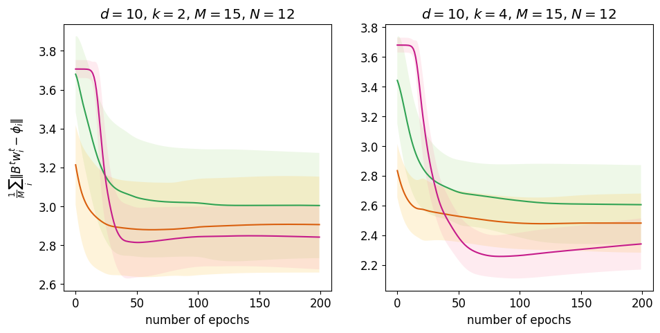
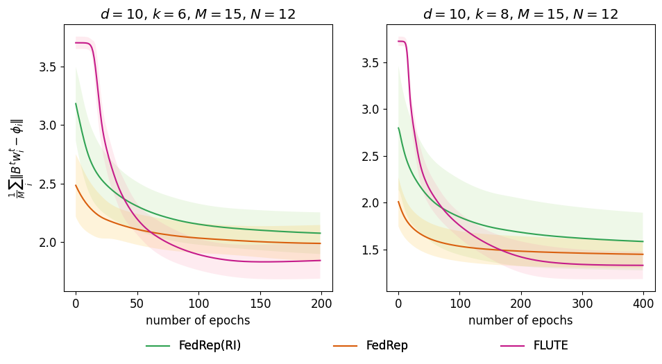
Figure 1: Experimental results with synthetic datasets.

7.2 Real World Datasets

Datasets and models. We now evaluate the performance of general FLUTE on multi-class classification tasks with real-world datasets CIFAR-10 and CIFAR-100 (Krizhevsky et al., 2009). For all experiments, we adopt a convolutional neural network (CNN) with two convolution layers, two fully connected layers with ReLU activation, and a final fully connected layer with a softmax activation function. A detailed description of the CNN structure is deferred to Appendix C of the Appendix.

Algorithms for comparison. We compare FLUTE with several baseline algorithms, including FedAvg (McMahan et al., 2017), Fed-LG (Liang et al., 2020), FedPer (Arivazhagan et al., 2019), FedRep (Collins et al., 2021), FedRod (Chen & Chao, 2021) and FedCP (Zhang et al., 2023a). Fed-LG is designed to learn a common head shared across clients while allowing for localized representations, while FedPer and FedRep both assume shared representation and personalized local heads. FedRod extends the model considered in FedRep by adding another head layer into the local model, and FedCP further equips a conditional policy network into the local model. We also consider variants of FLUTE and FedRep, denoted as FLUTE* and FedRep*, respectively, under which we vary the number of updates of the local heads in each communication round, as elaborated later.

Loss function and penalty. For algorithms other than FLUTE and FLUTE*, the local loss function is chosen as $\mathcal{L}_{i}=\frac{1}{N}\sum_{(x,y)\in\mathcal{D}_{i}}\mathcal{L}_{\text{CE}}(\mathbf{H}_{i}^{\top}\psi_{\mathbf{B}}(x)+b_{i},y)$, where $\mathcal{L}_{\text{CE}}$ is the cross entropy loss. The local loss function for FLUTE and FLUTE* are specialized as

$$\mathcal{L}_{i}(\mathbf{B},b,\mathbf{H})=\frac{1}{N}\sum_{(x,y)\in\mathcal{D}_{i}}\mathcal{L}_{\text{CE}}\big{(}\mathbf{H}_{i}^{\top}\psi_{\mathbf{B}}(x)+b_{i},y\big{)}+\quad\lambda_{1}\|\psi_{\mathbf{B}}(x)\|^{2}+\lambda_{2}\|\mathbf{H}_{i}\|_{F}^{2}+\lambda_{3}\mathcal{N}\mathcal{C}_{i}(\mathbf{H}_{i}),$$ (11)

where $y\in\mathbb{R}^{m}$ is a one-hot vector whose $k$-th entry is $1$ if the corresponding $x$ belongs to class $k$, $\lambda_{1}$, $\lambda_{2}$ and $\lambda_{3}$ are non-negative regularization parameters. $\mathcal{N}\mathcal{C}_{i}(\mathbf{H}_{i})$ is motivated by Papyan et al. (2020) and set as

$$\mathcal{N}\mathcal{C}_{i}(\mathbf{H}_{i})=\mathinner{\!\left\lVert\frac{\mathbf{H}^{\top}_{i}\mathbf{H}_{i}}{\|\mathbf{H}^{\top}_{i}\mathbf{H}_{i}\|_{F}}-\frac{1}{\sqrt{m-1}}\mathbf{u}_{i}\mathbf{u}_{i}^{\top}\odot\left(\mathbf{I}_{m}-\frac{1}{m}\mathbf{1}_{m}\mathbf{1}^{\top}_{m}\right)\right\rVert}_{F},$$

where $\mathbf{u}_{i}$ is an $m$-dimensional one-hot vector whose $c$-th entry is $1$ if $c\in\mathcal{C}_{i}$, and $\odot$ denotes the Hadamard product. We specialize the regularization term optimized on the server side as $R(\{\mathbf{H}_{i}\})=\sum_{i}\mathcal{N}\mathcal{C}_{i}(\mathbf{H}_{i})$. Note that for general FLUTE specified to a classification problem, we penalize $\|\psi_{\mathbf{B}}(x)\|$ instead of directly penalizing the parameter $\mathbf{B}$. Since $\|\psi_{\mathbf{B}}(x)\|^{2}$ depends on data, the regularization term is optimized partially on the client side and partially on the server side.

Compared with the objective function in Equation 4 for the linear case, the term $\lambda_{3}\mathcal{N}\mathcal{C}_{i}(\mathbf{H}_{i})$ replaces term (I) and $\lambda_{1}\|\psi_{\mathbf{B}}(x)\|^{2}+\lambda_{2}\|\mathbf{H}_{i}\|_{F}^{2}$ replaces term (II). The primary goal of introducing $\lambda_{3}\mathcal{N}\mathcal{C}_{i}(\mathbf{H}_{i})$ is to mitigate local over-fitting that occurs during local updates in the training process. As elaborated in Section B.3, such a regularization term promotes a beneficial structure for the global model, facilitating efficient learning performance. This term shares the same motivation as the term (I) in the linear scenario, which focuses on distilling significant components from the model to mitigate local over-fitting effects. For term (II), we only replace $\|\mathbf{B}^{\top}\mathbf{B}\|_{F}^{2}$ with $\|\psi_{\mathbf{B}}(x)\|^{2}$, since the representation is not linear in general.

Table 1: Average test accuracy on CIFAR-10 and CIFAR-100.

Dataset	CIFAR-10				CIFAR-100
Partition	50 $\times$ 2	50 $\times$ 5	100 $\times$ 2	100 $\times$ 5	100 $\times$ 5	100 $\times$ 10	100 $\times$ 20	100 $\times$ 40
FedAvg	34.460$\pm$1.083	47.217$\pm$0.395	41.584$\pm$0.433	51.876$\pm$0.675	20.212$\pm$0.574	31.533$\pm$0.519	34.659$\pm$0.482	32.902$\pm$0.195
FedAvg-FT	83.996$\pm$0.948	71.465$\pm$0.701	84.688$\pm$0.437	70.884$\pm$0.697	78.342$\pm$0.574	66.660$\pm$0.370	54.464$\pm$0.178	44.858$\pm$0.119
Fed-LG	82.724$\pm$2.137	61.820$\pm$0.409	83.019$\pm$0.431	62.957$\pm$0.895	72.526$\pm$0.692	53.526$\pm$0.151	34.445$\pm$0.375	22.702$\pm$0.315
FedPer	85.173$\pm$1.082	74.015$\pm$0.724	86.168$\pm$0.703	73.666$\pm$0.281	76.001$\pm$0.454	67.100$\pm$0.229	56.066$\pm$0.389	44.689$\pm$0.411
FedRep	86.133$\pm$0.775	71.737$\pm$0.296	86.685$\pm$0.766	73.808$\pm$0.561	78.621$\pm$0.159	68.530$\pm$0.255	56.360$\pm$0.245	43.061$\pm$0.476
FedRep*	87.320$\pm$1.485	75.766$\pm$0.220	87.177$\pm$0.489	75.296$\pm$0.505	78.892$\pm$0.410	68.630$\pm$0.705	56.654$\pm$0.609	42.025$\pm$0.404
FedRoD	79.476$\pm$2.966	68.728$\pm$1.750	83.296$\pm$1.545	72.116$\pm$0.788	74.299$\pm$0.338	66.462$\pm$0.284	57.280$\pm$0.105	48.120$\pm$0.186
FedCP	85.361$\pm$1.605	71.603$\pm$0.885	84.798$\pm$0.489	71.344$\pm$0.587	74.266$\pm$0.559	66.426$\pm$0.372	57.067$\pm$0.483	43.638$\pm$0.415
FLUTE	87.012$\pm$0.453	76.478$\pm$0.484	86.128$\pm$1.007	76.918$\pm$0.712	77.750$\pm$0.615	70.598$\pm$0.282	59.243$\pm$0.334	48.169$\pm$0.597
FLUTE*	87.713$\pm$1.365	76.543$\pm$0.921	88.567$\pm$0.457	78.255$\pm$0.688	79.560$\pm$0.627	70.844$\pm$0.419	59.714$\pm$0.448	48.170$\pm$0.440

Implementation and evaluation. We use $m$ to denote the number of classes assigned to each client. For CIFAR-10 dataset, we consider four $(N,m)$ pairs: $(50,2)$, $(50,5)$, $(100,2)$ and $(100,5)$; For CIFAR-100 dataset, we consider four $(N,m)$ pairs: $(100,5)$, $(100,10)$, $(100,20)$ and $(100,40)$.

For experiments conducted on the CIFAR-10 dataset, all algorithms are executed over 100 communication rounds. For LG-Fed, FedPer, FedRoD, FedCP and FLUTE, each client performs one round of local updates in each communication round. FedRep performs one epoch of local head update and an additional epoch for the local representation update. Compared with FedRep, FedRep* processes 10 epochs to update its local heads and one epoch to update its representation. For comparison, FLUTE* also runs 11 rounds of local updates, updating both representation and local head in the first round, followed by 10 rounds of only updating the local head.

The experiments on the CIFAR-100 dataset also use 100 communication rounds. The number of local updates for LG-Fed, FedPer, FedRoD, FedCP and FLUTE are set to 5. FedRep is configured to update the local representation and head for 5 epochs each, while FedRep* allocates 5 epochs for updating the local representation and 10 for updating the local head. FLUTE* runs 15 epochs of local updates, where the initial 5 epochs update both the representation and local head while the subsequent 10 epochs solely update the local head.

Averaged performance. The results are reported in Table 1. It is evident that FLUTE and FLUTE* consistently outperform other baseline algorithms in all experiments conducted on CIFAR-10 and CIFAR-100 datasets. This superior performance is attributed to the tailored design that encourages the locally learned models to move towards a global optimal solution rather than a local optimum. We also observe that the gain of FLUTE and FLUTE* becomes more prominent with larger $N$ and $m$. Intuitively, larger $N$ and $m$ implies more severe under-parameterization for the given CNN model, and our algorithms exhibit more advantage for such cases.

8 Conclusion

To the best of our knowledge, this paper represents the first effort in the study of federated representation learning in the under-parameterized regime, which is of great practical importance. We have proposed a novel FRL algorithm FLUTE that was inspired by asymmetric low-rank matrix approximation. FLUTE incorporates a novel regularization term in the loss function and solves the corresponding ERM problem in a federated manner. We proved the convergence of FLUTE and established the per-client sample complexity that is comparable to the over-parameterized result but with very different proof techniques. We also extended FLUTE to general (non-linear) settings which are of practical interest. FLUTE demonstrated superior performance over existing FRL solutions in both synthetic and real-world tasks, highlighting its advantages for efficient learning in the under-parameterized regime.

Notations. Throughout this paper, bold capital letters (e.g., $\mathbf{X}$) denote matrices, and calligraphic capital letters (e.g., $\mathcal{C}$) denote sets. We use $\text{tr}(\mathbf{X})$ to denote the trace of matrix $\mathbf{X}$, $\sigma_{\min}(\mathbf{X})$ and $\sigma_{\max}(\mathbf{X})$ to denote the minimum and maximum singular values of $\mathbf{X}$, respectively, and $\mathop{\mbox{\rm diag}}(x_{1},\cdots,x_{d})$ to denote a $d$-dimensional diagonal matrix with diagonal entries $x_{1},\cdots,x_{d}$. $|\mathcal{C}|$ denotes the cardinality of set $\mathcal{C}$, and $\{X_{i}\}_{i\in[N]}$ denotes the set $\{X_{1},\cdots,X_{N}\}$. We use $\langle x,y\rangle$ to denote the inner product of $x$ and $y$, and $\|x\|$ to denote the Euclidean norm of vector $x$. We use $f\circ\psi$ to denote the composition of functions $f\mathrel{\mathop{\mathchar 58\relax}}\mathbb{R}^{k}\rightarrow\mathbb{R}^{m}$ and $\psi\mathrel{\mathop{\mathchar 58\relax}}\mathbb{R}^{d}\rightarrow\mathbb{R}^{k}$, i.e., $(f\circ\psi)(x)=f(\psi(x))$. $a\lesssim b$ indicates $a\leq Cb$ for a positive constant $C$. $\mathbf{I}_{d}$ represents a $d\times d$ identity matrix, and $\mathbf{0}$ is a $d$-dimensional all-zero vector.

Denote ${\overline{d}}\mathrel{\mathop{\mathchar 58\relax}}=\max\{d,M\}$, ${\underline{d}}\mathrel{\mathop{\mathchar 58\relax}}=\min\{d,M\}$, and $\mathbf{\Phi}_{\star}\in\mathbb{R}^{{\overline{d}}\times{\overline{d}}}$ as the matrix constructed from $\mathbf{\Phi}\in\mathbb{R}^{d\times M}$ by padding all-zero columns or rows. Define its SVD as $\mathbf{\Phi}_{\star}=\mathbf{U}_{\star}\mathbf{\Lambda}_{\star}\mathbf{V}^{\top}_{\star}$. Denote $\tilde{\mathbf{\Lambda}}=\mathop{\mbox{\rm diag}}(2\mathbf{\Lambda}_{\star},-2\mathbf{\Lambda}_{\star})$ and let $\lambda_{1}^{*}\geq\lambda_{2}^{*}\geq\cdots\geq\lambda_{2{\overline{d}}}^{*}$ be the eigenvalues of $\tilde{\mathbf{\Lambda}}$, with $\Delta=\lambda_{k}^{*}-\lambda_{k+1}^{*}$. Note that the definition of $\Delta$ is consistent with the definition in Section 5. For clarity of presentation, we use $\sigma_{\xi}$ to denote the standard deviation of the noise $\xi$ instead of $\sigma$ that is used in the main paper.

Appendix A Analysis of the FLUTE Linear Algorithm

A.1 Preliminaries

We start with the updating rule of $\mathbf{B}^{t}$ and $\mathbf{W}^{t}$ in Algorithm 1.

For $\mathbf{B}^{t}$, from FLUTE we have the following updating rule:

$${\mathbf{B}}^{t+1} =\mathbf{B}^{t}-\frac{{\eta}}{N}\sum_{i\in[M]}\sum_{j\in[N]}x_{i,j}\big{(}x_{i,j}^{\top}\mathbf{B}^{t}{w}_{i}^{t}-y_{i,j}\big{)}({w}_{i}^{t})^{\top}-\frac{\eta}{2}\mathbf{B}^{t}\big{(}(\mathbf{B}^{t})^{\top}\mathbf{B}^{t}-\mathbf{W}^{t}(\mathbf{W}^{t})^{\top}\big{)}$$

$$=\mathbf{B}^{t}-\frac{{\eta}}{N}\sum_{i\in[M]}\mathbf{X}_{i}\mathbf{X}_{i}^{\top}\big{(}\mathbf{B}^{t}{w}_{i}^{t}-\phi_{i}\big{)}({w}_{i}^{t})^{\top}-\frac{\eta}{2}\mathbf{B}^{t}\big{(}(\mathbf{B}^{t})^{\top}\mathbf{B}^{t}-\mathbf{W}^{t}(\mathbf{W}^{t})^{\top}\big{)}.$$

Since data points $\{x_{i,j}\}$ are sampled from a standard Gaussian distribution, for large $N$, it holds that $\mathbf{X}_{i}\mathbf{X}_{i}^{\top}/N\approx\mathbf{I}$. Then, we introduce the following definition:

$$\mathbf{Q}^{t+1}\coloneqq\eta\sum_{i\in[M]}\big{(}\mathbf{B}^{t}{w}_{i}^{t}-\phi_{i}\big{)}({w}_{i}^{t})^{\top}-\eta\sum_{i\in[M]}\frac{\mathbf{X}_{i}\mathbf{X}_{i}^{\top}}{N}\big{(}\mathbf{B}^{t}{w}_{i}^{t}-\phi_{i}\big{)}({w}_{i}^{t})^{\top}+\eta\sum_{i\in[M]}\frac{\mathbf{X}_{i}\mathbf{E}_{i}({w}_{i}^{t})^{\top}}{N}.$$ (12)

With this definition, the updating rule of $\mathbf{B}^{t}$ can be rewritten as

$${\mathbf{B}}^{t+1}=\mathbf{B}^{t}-\eta\big{(}\mathbf{B}^{t}\mathbf{W}^{t}-\mathbf{\Phi}\big{)}(\mathbf{W}^{t})^{\top}-\frac{\eta}{2}\mathbf{B}^{t}\big{(}(\mathbf{B}^{t})^{\top}\mathbf{B}^{t}-\mathbf{W}^{t}(\mathbf{W}^{t})^{\top}\big{)}+\mathbf{Q}^{t+1}.$$

Now we consider the updating rule of $\mathbf{W}$. Observe that each of its columns satisfies

$$w_{i}^{t+1} =w_{i}^{t}-\frac{\eta}{N}\sum_{j\in[N]}(\mathbf{B}^{t})^{\top}x_{i,j}\big{(}(x_{i,j})^{\top}\mathbf{B}^{t}{w}_{i}^{t}-y_{i,j}\big{)}$$

$$=w_{i}^{t}-\frac{\eta}{N}(\mathbf{B}^{t})^{\top}\mathbf{X}_{i}\mathbf{X}_{i}^{\top}\big{(}\mathbf{B}^{t}{w}_{i}^{t}-\phi_{i}\big{)}.$$

We define $\tilde{\mathbf{Q}}^{t+1}\coloneqq[\tilde{q}_{1}^{t+1},\cdots,\tilde{q}_{M}^{t+1}]$, where each of its columns is given by

$$\tilde{q}_{i}^{t+1}\coloneqq\eta(\mathbf{B}^{t})^{\top}\big{(}\mathbf{B}^{t}w_{i}^{t}-\phi_{i}\big{)}-\frac{\eta}{N}(\mathbf{B}^{t})^{\top}\mathbf{X}_{i}\mathbf{X}_{i}^{\top}\big{(}\mathbf{B}^{t}w_{i}^{t}-\phi_{i}\big{)}+\frac{\eta}{N}(\mathbf{B}^{t})^{\top}\mathbf{X}_{i}\mathbf{E}_{i}.$$ (13)

Then, $\mathbf{W}^{t}$ is updated according to

$$\mathbf{W}^{t+1}=\mathbf{W}^{t}-\eta(\mathbf{B}^{t})^{\top}(\mathbf{B}^{t}\mathbf{W}^{t}-\mathbf{\Phi})+\frac{\eta}{2}\big{(}(\mathbf{B}^{t})^{\top}\mathbf{B}^{t}-\mathbf{W}^{t}(\mathbf{W}^{t})^{\top}\big{)}\mathbf{W}^{t}+\tilde{\mathbf{Q}}^{t+1}.$$

Recall the SVD of $\mathbf{\Phi}$ is denoted as $\mathbf{\Phi}=\mathbf{U}\mathbf{\Lambda}\mathbf{V}^{\top}$. Further denote $\tilde{\mathbf{B}}^{t}=\mathbf{U}^{\top}\mathbf{B}^{t}$ and $\tilde{\mathbf{W}}^{t}=\mathbf{W}^{t}\mathbf{V}$. Then, we have

$$\tilde{\mathbf{B}}^{t+1} =\tilde{\mathbf{B}}^{t}-\eta\big{(}\tilde{\mathbf{B}}^{t}\tilde{\mathbf{W}}^{t}-\mathbf{\Lambda}\big{)}\big{(}\tilde{\mathbf{W}}^{t}\big{)}^{\top}-\frac{\eta}{2}\tilde{\mathbf{B}}^{t}\big{(}(\tilde{\mathbf{B}}^{t})^{\top}\tilde{\mathbf{B}}^{t}-\tilde{\mathbf{W}}^{t-1}(\tilde{\mathbf{W}}^{t})^{\top}\big{)}+\mathbf{U}^{\top}\mathbf{Q}^{t+1},$$

$$\tilde{\mathbf{W}}^{t+1} =\tilde{\mathbf{W}}^{t}-\eta(\tilde{\mathbf{B}}^{t})^{\top}\big{(}\tilde{\mathbf{B}}^{t}\tilde{\mathbf{W}}^{t}-\mathbf{\Lambda}\big{)}-\frac{\eta}{2}\big{(}(\tilde{\mathbf{B}}^{t})^{\top}\tilde{\mathbf{B}}^{t}-\tilde{\mathbf{W}}^{t}(\tilde{\mathbf{W}}^{t})^{\top}\big{)}\tilde{\mathbf{W}}^{t}+\tilde{\mathbf{Q}}^{t+1}\mathbf{V}.$$

Similar to the definition of $\mathbf{\Phi}_{\star}$, we construct $\mathbf{B}^{t}_{\star}\in\mathbb{R}^{{\overline{d}}\times k}$ and $\mathbf{W}^{t}_{\star}\in\mathbb{R}^{k\times{\overline{d}}}$ by padding all-zero columns or rows to $\tilde{\mathbf{B}}^{t}$ and $\tilde{\mathbf{W}}$, respectively. Similarly, we obtain $\mathbf{Q}^{t}_{\star}\in\mathbb{R}^{{\overline{d}}\times k}$ and $\tilde{\mathbf{Q}}^{t}_{\star}\in\mathbb{R}^{k\times{\overline{d}}}$ by padding all-zero columns or rows to $\mathbf{Q}^{t}$ and $\tilde{\mathbf{Q}}^{t}$, respectively. Then, we define $\mathbf{\Theta}^{t}$ and $\mathbf{R}^{t}$ as

$$\mathbf{\Theta}^{t} =\bigg{[}\frac{(\mathbf{B}^{t}_{\star})^{\top}+\mathbf{W}_{\star}^{t}}{\sqrt{2}}\quad\frac{(\mathbf{B}^{t}_{\star})^{\top}-\mathbf{W}^{t}_{\star}}{\sqrt{2}}\bigg{]}^{\top},$$

$$\mathbf{R}^{t} =\bigg{[}\frac{(\mathbf{Q}^{t}_{\star})^{\top}\mathbf{U}_{\star}+\tilde{\mathbf{Q}}^{t}_{\star}\mathbf{V}_{\star}}{\sqrt{2}}\quad\frac{(\mathbf{Q}^{t}_{\star})^{\top}\mathbf{U}_{\star}-\tilde{\mathbf{Q}}^{t}_{\star}\mathbf{V}_{\star}}{\sqrt{2}}\bigg{]}^{\top}.$$

Then, the updating rule of $\mathbf{\Theta}^{t}$ can be described as

$$\mathbf{\Theta}^{t+1}=\mathbf{\Theta}^{t}+\frac{\eta}{2}\tilde{\mathbf{\Lambda}}\mathbf{\Theta}^{t}-\frac{\eta}{2}\mathbf{\Theta}^{t}(\mathbf{\Theta}^{t})^{\top}\mathbf{\Theta}^{t}+\mathbf{R}^{t+1}.$$ (14)

Let $\mathbf{\Theta}^{t}=[(\mathbf{\Theta}^{t}_{k})^{\top}(\mathbf{\Theta}^{t}_{\text{res}})^{\top}]^{\top}$ and $\mathbf{R}^{t}=[(\mathbf{R}^{t}_{k})^{\top}\quad(\mathbf{R}^{t}_{2{\overline{d}}-k})^{\top}]^{\top}$ where $\mathbf{\Theta}^{t}_{k}\in\mathbb{R}^{k\times k}$, $\mathbf{\Theta}^{t}_{\text{res}}\in\mathbb{R}^{(2{\overline{d}}-k)\times k}$, $\mathbf{R}^{t}_{k}\in\mathbb{R}^{k\times k}$ and $\mathbf{R}^{t}_{2{\overline{d}}-k}\in\mathbb{R}^{(2{\overline{d}}-k)\times k}$. Then, we decompose the updating rule of $\mathbf{\Theta}^{t}$ as

$$\mathbf{\Theta}^{t}_{k} =\mathbf{\Theta}^{t-1}_{k}+\frac{\eta}{2}\tilde{\mathbf{\Lambda}}_{k}\mathbf{\Theta}^{t-1}_{k}-\frac{\eta}{2}\mathbf{\Theta}^{t-1}_{k}(\mathbf{\Theta}^{t-1})^{\top}\mathbf{\Theta}^{t-1}+\mathbf{R}^{t}_{k},$$ (15)

$$\mathbf{\Theta}^{t}_{\text{res}} =\mathbf{\Theta}^{t-1}_{\text{res}}+\frac{\eta}{2}\tilde{\mathbf{\Lambda}}_{\text{res}}\mathbf{\Theta}^{t-1}_{\text{res}}-\frac{\eta}{2}\mathbf{\Theta}^{t-1}_{\text{res}}(\mathbf{\Theta}^{t-1})^{\top}\mathbf{\Theta}^{t-1}+\mathbf{R}^{t}_{2d-k}.$$ (16)

A.2 Proof of Theorem 5.5

First, we restate Theorem 5.5 as follows.

Theorem A.1 (Restatement of Theorem 5.5).

Set $\lambda$ and $\eta$ as in Theorem 5.1. Then for constant $T_{\mathcal{R}}$ and any $T>T_{\mathcal{R}}$, there exist positive constants $c_{1}$ and $c_{2}$ such that when the number of samples per client satisfies $N\geq c_{1}\frac{({\overline{d}}-\log\delta+\log T)(k\sqrt{(\lambda_{1}^{*})^{2}+E}+\sqrt{k}\sigma_{\xi})^{2}}{\kappa_{T}^{2}\Delta^{2}}$, for all $T_{\mathcal{R}}<t\leq T$ we have

$$\frac{1}{M}\sum_{i\in[M]}\|\mathbf{B}^{t}w^{t}_{i}-\mathbf{B}^{*}w_{i}^{*}\|\leq\frac{c_{2}\kappa\sqrt{k}}{\sqrt{M}}\Big{(}1-\frac{\eta\Delta}{16}\Big{)}^{t},$$

with probability at least $1-\delta$, where $\kappa_{T}=(1-\frac{\eta\Delta}{16})^{T}$.

Overview of the proof. The proof of Theorem 5.5 consists of three main steps.

• Step 1: We show that with a small random initialization, $\mathbf{\Theta}^{t}$ will enter a region containing the optima with high probability (see Section A.2.1).

• Step 2: We show that once $\mathbf{\Theta}^{t}$ enters this region, it will stay in it with high probability (see Section A.2.2).

• Step 3: We show that when $N$ is sufficiently large, with high probability it holds that $\|\mathbf{\Theta}^{t}(\mathbf{\Theta}^{t})^{\top}-\mathop{\mbox{\rm diag}}(\tilde{\mathbf{\Lambda}}_{k},\mathbf{0})\|$ converges to $0$ at a linear rate when the initialization satisfies $\mathbf{\Theta}^{0}\in\mathcal{R}$ (see Section A.2.3).

We then put pieces together and prove Theorem 5.5 in Section A.2.4. We introduce some auxiliary lemmas in Section A.2.5.

A.2.1 Step 1: Entering a Region with Small Random Initialization

We first introduce the following definitions, adapted from the proof in Chen et al. (2023). Recall that $\Delta=\lambda_{k}^{*}-\lambda_{k+1}^{*}$. We define

$$\mathcal{R} =\bigg{\{}\mathbf{\Theta}^{t}=\begin{bmatrix}\mathbf{\Theta}^{t}_{k}\\ \mathbf{\Theta}^{t}_{\text{res}}\end{bmatrix}\in\mathbb{R}^{2d\times k}\bigg{|}\sigma_{1}^{2}(\mathbf{\Theta}^{t})\leq 2\lambda_{1}^{*},\quad\sigma_{1}^{2}(\mathbf{\Theta}^{t}_{\text{res}})\leq\lambda^{*}_{k}-\Delta/2,\quad\sigma_{k}^{2}(\mathbf{\Theta}^{t}_{k})\geq\Delta/4\bigg{\}},$$

$$\mathcal{R}_{s} =\bigg{\{}\mathbf{\Theta}^{t}=\begin{bmatrix}\mathbf{\Theta}^{t}_{k}\\ \mathbf{\Theta}^{t}_{\text{res}}\end{bmatrix}\in\mathbb{R}^{2d\times k}\bigg{|}\sigma_{1}^{2}(\mathbf{\Theta}^{t})\leq 2\lambda_{1}^{*},\quad\sigma_{1}^{2}(\mathbf{\Theta}^{t}_{\text{res}})\leq\lambda^{*}_{k}-\Delta/2\bigg{\}}.$$

Then, we establish the following proposition.

Proposition A.2.

Assume $\eta\leq\frac{1}{6\lambda_{1}^{*}}$ and all entries of $\mathbf{B}^{0}$ and $\mathbf{W}^{0}$ are independently sampled from $\mathcal{N}(0,\alpha^{2})$ with a sufficiently small $\alpha$. Then, if

$$\sqrt{N}\geq\max\Bigg{\{}\frac{\sqrt{{\overline{d}}-\log\delta}}{\sqrt{c_{1}}},\frac{3456\sqrt{{\overline{d}}-\log\delta}\sqrt{\lambda_{1}^{*}}(\sqrt{k(\lambda_{1}^{*})^{2}+E}+\sqrt{k}\sigma_{\xi})}{\min\{\sigma_{1}(\mathbf{\Theta}_{\text{res}}^{0}),\sigma_{1}(\mathbf{\Theta}_{\text{res}}^{0})\}\Delta\sqrt{c_{1}}}\Bigg{\}},$$

with probability at least $1-ct\delta$ for some constant $c>0$, $\mathbf{\Theta}^{t}$ will enter region $\mathcal{R}$ for some $t\in[T_{\mathcal{R}}]$, where

$$T_{\mathcal{R}}=\frac{\log(\Delta/{(4\sigma_{k}^{2}(\mathbf{\Theta}_{k}^{0}))})}{2\log(1+\frac{\eta}{2}(\lambda_{k}^{*}-\Delta/2))}.$$ (17)

The proof of Proposition A.2 relies on Lemma A.4 and Lemma A.5, which will be introduced shortly. Before that, we state the following claim introduced in Chen et al. (2023):

Claim A.3.

$\sigma_{1}^{2}(\mathbf{\Theta}^{0})\leq\lambda_{1}^{*}$, $\sigma_{1}^{2}(\mathbf{\Theta}_{\text{res}}^{0})\leq\lambda_{k}^{*}-\Delta/2$, $\sigma_{k}^{2}(\mathbf{\Theta}_{k}^{0})\leq\Delta/4$ and $\sigma_{1}^{2}(\mathbf{\Theta}_{\text{res}}^{0})\leq c_{1}\cdot\sigma_{k}(\mathbf{\Theta}_{k}^{0})^{1+\kappa},$ where $c_{1}=\frac{\Delta^{1-\kappa/2}}{2^{3-\kappa}}$ and $\kappa=\frac{\log(1+\frac{\eta}{2}\lambda_{k+1}^{*}+\frac{\eta}{8}\Delta)}{\log(1+\frac{\eta}{2}(\lambda_{k}^{*}-\Delta/2))}<1$.

The following lemma shows that with a small random initialization, A.3 holds with high probability.

Lemma A.4.

Assume all entries of $\mathbf{B}^{0}$ and $\mathbf{W}^{0}$ are independently sampled from $\mathcal{N}(0,\alpha^{2})$. Then, for any $\delta\in[0,1]$, if $\alpha$ is sufficiently small, A.3 holds with probability at least $1-\delta$.

Proof of Lemma A.4.

Using Lemma A.19, we have $\sigma_{1}(\mathbf{\Theta}^{0})\leq\sqrt{\lambda_{1}^{*}}$ and $\sigma_{1}(\mathbf{\Theta}_{\text{res}}^{0})\leq\sqrt{\lambda_{k}^{*}-\Delta/2}$ hold with probability at least $1-2\exp(-(\frac{1}{\alpha^{2}}\sqrt{\lambda_{k}^{*}-\Delta/2}-2\sqrt{d})^{2}/2)$, and $\sigma_{k}(\mathbf{\Theta}_{k}^{0})\leq\sqrt{\Delta}/2$ holds with probability at least $1-2\exp(-(\sqrt{\Delta}/(2\alpha^{2})-2\sqrt{d})^{2}/2)$. Then for $\alpha$ small enough such that

$$\alpha\leq\min\Big{\{}\frac{\sqrt{\Delta}}{4\sqrt{d}+2\sqrt{2\log(2/\delta^{\prime})}},\;\frac{\sqrt{\lambda_{1}^{*}-\Delta/2}}{2\sqrt{d}+\sqrt{2\log(2/\delta^{\prime})}}\Big{\}},$$

$\sigma_{1}(\mathbf{\Theta}^{0})\leq\sqrt{\lambda_{1}^{*}}$, $\sigma_{1}(\mathbf{\Theta}_{\text{res}}^{0})\leq\sqrt{\lambda_{k}^{*}-\Delta/2}$ and $\sigma_{k}(\mathbf{\Theta}_{k}^{0})\leq\sqrt{\Delta}/2$ hold with probability at least $1-2\delta^{\prime}$ for any $\delta^{\prime}\in[0,1]$.

From Rudelson & Vershynin (2008), there exists a constant $K$ that only depends on $\delta^{\prime}$ such that with probability at least $1-\delta^{\prime}$, we have $\sigma_{k}(\mathbf{\Theta}_{k}^{0})\geq{\alpha^{2}}{K\sqrt{k}}$.

Thus, when $\alpha$ is sufficiently small such that $\alpha^{4-2(1+\kappa)}\leq\frac{c_{1}(K\sqrt{k})^{1+\kappa}}{8d+4\log(2/\delta^{\prime})}$, with probability at least $1-\delta^{\prime}$, we have

$$c_{1}\sigma_{k}(\mathbf{\Theta}_{k}^{0})^{1+\kappa}\geq c_{1}(\alpha^{2}K\sqrt{k})^{1+\kappa}\geq\alpha^{4}(2\sqrt{d}+\sqrt{2\log(2/\delta^{\prime})})^{2}.$$

Note that from Lemma A.19, with probability at least $1-\delta^{\prime}$ we have

$$\sigma_{1}^{2}(\mathbf{\Theta}_{\text{res}}^{0})\leq\alpha^{4}(2\sqrt{d}+\sqrt{2\log(2/{\delta^{\prime}})})^{2}.$$

Then we conclude that with probability at least $1-4\delta^{\prime}$, we have $\sigma_{1}(\mathbf{\Theta}^{0})\leq\sqrt{\lambda_{1}^{*}}$, $\sigma_{1}(\mathbf{\Theta}^{0}_{\text{res}})\leq\sqrt{\lambda_{1}^{*}-\Delta/2}$, $\sigma_{k}(\mathbf{\Theta}_{k}^{0})\leq\sqrt{\Delta}/2$ and $\sigma_{1}^{2}(\mathbf{\Theta}_{\text{res}}^{0})\leq c_{1}\cdot\sigma_{k}(\mathbf{\Theta}_{k}^{0})^{1+\kappa}$. Finally the lemma follows by setting $\delta=4\delta^{\prime}$. ∎

Next, we introduce the following lemma, which shows that when A.3 holds, $\mathbf{\Theta}^{t}$ will enter the region $\mathcal{R}$ in a short time period.

Lemma A.5.

Assume $\eta\leq\frac{1}{6\lambda_{1}^{*}}$ and A.3 holds. Then, if

$$\sqrt{N}\geq\max\Big{\{}\frac{\sqrt{{\overline{d}}-\log\delta}}{\sqrt{c_{1}}},\frac{3456\sqrt{{\overline{d}}-\log\delta}\sqrt{\lambda_{1}^{*}}(\sqrt{k(\lambda_{1}^{*})^{2}+E}+\sqrt{k}\sigma_{\xi})}{\min\{\sigma_{1}(\mathbf{\Theta}_{\text{res}}^{0}),\sigma_{1}(\mathbf{\Theta}_{\text{res}}^{0})\}\Delta\sqrt{c_{1}}}\Big{\}},$$ (18)

with probability at least $1-ct\delta$, we have $\sigma_{k}(\mathbf{\Theta}^{t}_{k})\geq\sqrt{\Delta}/2$ for some $t\in[0,\frac{\log(\Delta/{4\sigma_{k}^{2}(\mathbf{\Theta}_{k}^{0})})}{2\log(1+\frac{\eta}{2}(\lambda_{k}^{*}-\Delta/2))}]$.

Proof of Lemma A.5.

With A.3 holds, we have $\sigma_{1}^{2}(\mathbf{\Theta}^{0})\leq 2\lambda_{1}^{*}$, $\sigma_{1}^{2}(\mathbf{\Theta}_{\text{res}}^{0})\leq\lambda^{*}_{k}-\Delta/2$. Then, based on Lemma A.17, for $N$ satisfying inequality (18), we have

$$\sigma_{1}(\mathbf{\Theta}^{t}_{\text{res}})\leq\Big{(}1+\frac{\eta}{2}\lambda^{*}_{k+1}+\frac{\eta}{8}\Delta\Big{)}^{t}\sigma_{1}(\mathbf{\Theta}^{0}_{\text{res}}),$$

holds with probability at least $1-ct\delta$. Combining with A.3, we obtain

$$\Big{(}1+\frac{\eta}{2}\lambda_{k+1}^{*}+\frac{\eta}{8}\Delta\Big{)}^{T_{\mathcal{R}}}\sigma_{1}^{2}(\mathbf{\Theta}_{\text{res}}^{0})=\Big{(}\frac{\Delta}{4\sigma_{k}^{2}(\mathbf{\Theta}_{k}^{0})}\Big{)}^{\kappa/2}\sigma_{1}^{2}(\mathbf{\Theta}_{\text{res}}^{0})\leq\frac{\Delta}{8\sqrt{\lambda_{1}^{*}}}\sigma_{k}(\mathbf{\Theta}_{k}^{0}).$$

Then, for all $t\leq T_{\mathcal{R}}$, we have

$$\Big{(}1+\frac{\eta}{2}\lambda_{k+1}^{*}+\frac{\eta}{8}\Delta\Big{)}^{2t}\sigma_{1}^{2}(\mathbf{\Theta}_{\text{res}}^{0})\leq\Big{(}1+\frac{\eta}{2}\lambda_{k+1}^{*}+\frac{\eta}{8}\Delta\Big{)}^{t+T_{\mathcal{R}}}\sigma_{1}^{2}(\mathbf{\Theta}_{\text{res}}^{0})\leq\Big{(}1+\frac{\eta}{2}\lambda_{k}^{*}-\frac{\eta}{4}\Delta\Big{)}^{t}\frac{\Delta}{8\sqrt{\lambda_{1}^{*}}}\sigma_{k}(\mathbf{\Theta}_{k}^{0}).$$

Let $T^{\prime}=\min\{t>0|\sigma_{k}^{2}(\mathbf{\Theta}_{k}^{t})\geq\Delta/4\}$. We then aim to prove that

$$\sigma_{k}(\mathbf{\Theta}_{k}^{t})\geq\Big{(}1+\frac{\eta}{2}\lambda_{k}^{*}-\frac{\eta}{4}\Delta\Big{)}^{t}\sigma_{k}(\mathbf{\Theta}_{k}^{0}),\quad\forall t\leq\min\{T_{\mathcal{R}},T^{\prime}\}.$$ (19)

We prove it by induction.

Assume Equation 19 holds for some $\tau\leq t$, where $t\leq\min\{T_{\mathcal{R}},T^{\prime}\}$. Then we have

$$\sigma_{1}^{2}(\mathbf{\Theta}_{\text{res}}^{\tau})\leq\Big{(}1+\frac{\eta}{2}\lambda_{k+1}^{*}+\frac{\eta}{8}\Delta\Big{)}^{2\tau}\sigma_{1}^{2}(\mathbf{\Theta}^{0}_{\text{res}})\leq\frac{\Delta}{8\sqrt{\lambda_{1}^{*}}}\Big{(}1+\frac{\eta}{2}\lambda_{k+1}^{*}-\frac{\eta}{4}\Delta\Big{)}^{\tau}\sigma_{k}(\mathbf{\Theta}_{k}^{0})\leq\frac{\Delta}{8\sqrt{\lambda_{1}^{*}}}\sigma_{k}(\mathbf{\Theta}^{\tau}_{k}).$$

We consider the next time step $\tau+1$. Note that $\sigma_{k}(\mathbf{\Theta}^{\tau+1}_{k})$ can be lower bounded as

$$\sigma_{k}(\mathbf{\Theta}^{\tau+1}_{k}) \geq\sigma_{k}(\mathbf{\Theta}^{\tau}_{k}+\frac{\eta}{2}\tilde{\mathbf{\Lambda}}_{k}\mathbf{\Theta}^{\tau}_{k}-\frac{\eta}{2}\mathbf{\Theta}^{\tau}_{k}(\mathbf{\Theta}^{\tau})^{\top}\mathbf{\Theta}^{\tau})-\sigma_{1}(\mathbf{R}^{\tau+1}_{k})$$

$$\geq\sigma_{k}(\mathbf{\Theta}^{\tau}_{k}+\frac{\eta}{2}\tilde{\mathbf{\Lambda}}_{k}\mathbf{\Theta}^{\tau}_{k}-\frac{\eta}{2}\mathbf{\Theta}^{\tau}_{k}(\mathbf{\Theta}^{\tau}_{k})^{\top}\mathbf{\Theta}^{\tau}_{k})-\frac{\eta}{2}\sigma_{1}(\mathbf{\Theta}_{k}^{\tau}(\mathbf{\Theta}^{\tau}_{\text{res}})^{\top}\mathbf{\Theta}^{\tau}_{\text{res}})-\sigma_{1}(\mathbf{R}^{\tau+1}).$$

Applying Lemma D.4 in Jiang et al. (2022) gives

$$\sigma_{k}(\mathbf{\Theta}^{\tau}_{k}+\frac{\eta}{2}\tilde{\mathbf{\Lambda}}_{k}\mathbf{\Theta}^{\tau}_{k}-\frac{\eta}{2}\mathbf{\Theta}^{\tau}_{k}(\mathbf{\Theta}^{\tau}_{k})^{\top}\mathbf{\Theta}^{\tau}_{k})-\frac{\eta}{2}\sigma_{1}(\mathbf{\Theta}_{k}^{\tau}(\mathbf{\Theta}^{\tau}_{\text{res}})^{\top}\mathbf{\Theta}^{\tau}_{\text{res}})$$

$$\geq\big{(}1-\frac{(\eta)^{2}}{2}\sigma_{1}(\tilde{\mathbf{\Lambda}}_{k}(\mathbf{\Theta}^{\tau}_{k})^{\top}\mathbf{\Theta}^{\tau}_{k})\big{)}(1+\frac{\eta}{2}\lambda_{k}^{*})\sigma_{k}(\mathbf{\Theta}_{k}^{\tau})\big{(}1-\frac{\eta}{2}\sigma_{k}^{2}(\mathbf{\Theta}_{k}^{\tau})\big{)}-\frac{\eta}{2}\sigma_{1}(\mathbf{\Theta}_{k}^{\tau}(\mathbf{\Theta}^{\tau}_{\text{res}})^{\top}\mathbf{\Theta}^{\tau}_{\text{res}})$$

$$\geq\Big{(}1-\frac{(\eta)^{2}}{2}{\lambda_{1}^{*}}^{2}\Big{)}\Big{(}1+\frac{\eta\lambda_{k}^{*}}{2}\Big{)}\Big{(}1-\frac{\eta\Delta}{4}\Big{)}\sigma_{k}(\mathbf{\Theta}_{k}^{\tau})-\frac{\eta\Delta}{8}\sigma_{k}(\mathbf{\Theta}_{k}^{\tau}).$$

Then, for $\eta\leq\frac{\Delta^{2}}{18{\lambda_{1}^{*}}^{3}}$, we have

$$\sigma_{k}(\mathbf{\Theta}^{\tau}_{k}+\frac{\eta}{2}\tilde{\mathbf{\Lambda}}_{k}\mathbf{\Theta}^{\tau}_{k}-\frac{\eta}{2}\mathbf{\Theta}^{\tau}_{k}(\mathbf{\Theta}^{\tau}_{k})^{\top}\mathbf{\Theta}^{\tau}_{k})-\frac{\eta}{2}\sigma_{1}(\mathbf{\Theta}_{k}^{\tau}(\mathbf{\Theta}^{\tau}_{\text{res}})^{\top}\mathbf{\Theta}^{\tau}_{\text{res}})\geq\Big{(}1+\frac{\eta\lambda_{k}^{*}}{2}-\eta\Delta\frac{71}{288}\Big{)}\sigma_{k}(\mathbf{\Theta}_{k}^{\tau}).$$ (20)

According to Lemma A.13 and Lemma A.14, if

$$\sqrt{N}\geq\max\Big{\{}\frac{\sqrt{{\overline{d}}-\log\delta}}{\sqrt{c_{1}}},\frac{3456\sqrt{\lambda_{1}^{*}}(\sqrt{k(\lambda_{1}^{*})^{2}+E}+\sqrt{k}\sigma_{\xi})\sqrt{{\overline{d}}-\log\delta}}{\sigma_{k}(\mathbf{\Theta}_{k}^{0})\Delta\sqrt{c_{1}}}\Big{\}},$$

then, with probability at least $1-2\delta$, we have $\sigma_{1}(\mathbf{R}^{\tau+1})\leq\frac{1}{288}\eta\Delta\sigma_{k}(\mathbf{\Theta}_{k}^{0})$.

Combining with Equation 20 gives

$$\sigma_{k}(\mathbf{\Theta}^{\tau+1}_{k}) \geq\Big{(}1+\frac{\eta\lambda_{k}^{*}}{2}-\eta\Delta\frac{71}{288}\Big{)}\sigma_{k}(\mathbf{\Theta}_{k}^{\tau})-\frac{1}{288}\eta\Delta\sigma_{k}(\mathbf{\Theta}_{k}^{0})$$

$$\geq\Big{(}1+\frac{\eta\lambda_{k}^{*}}{2}-\eta\Delta\frac{71}{288}\Big{)}\Big{(}1+\frac{\eta}{2}\lambda_{k}^{*}-\frac{\eta}{4}\Delta\Big{)}^{\tau}\sigma_{k}(\mathbf{\Theta}_{k}^{0})-\frac{1}{288}\eta\Delta\sigma_{k}(\mathbf{\Theta}_{k}^{0})$$

$$\geq\Big{(}1+\frac{\eta\lambda_{k}^{*}}{2}-\eta\Delta\frac{71}{288}\Big{)}\Big{(}1+\frac{\eta}{2}\lambda_{k}^{*}-\frac{\eta}{4}\Delta\Big{)}^{\tau}\sigma_{k}(\mathbf{\Theta}_{k}^{0})-\frac{1}{288}\Big{(}1+\frac{\eta}{2}\lambda_{k}^{*}-\frac{\eta}{4}\Delta\Big{)}^{\tau}\eta\Delta\sigma_{k}(\mathbf{\Theta}_{k}^{0})$$

$$=\Big{(}1+\frac{\eta}{2}\lambda_{k}^{*}-\frac{\eta}{4}\Delta\Big{)}^{\tau+1}\sigma_{k}(\mathbf{\Theta}_{k}^{0}).$$

Then, we conclude that with probability at least $1-ct\delta$ for some constant $c$, we have

$$\sigma_{k}(\mathbf{\Theta}^{t}_{k})\geq\Big{(}1+\eta\lambda_{k}^{*}/2-\eta\Delta/4\Big{)}^{t}\sigma_{k}(\mathbf{\Theta}_{k}^{0}).$$

Here we claim $T_{\mathcal{R}}\leq T^{\prime}$ always holds, since if $T_{\mathcal{R}}>T^{\prime}$, we must have

$$\sigma_{k}(\mathbf{\Theta}^{T_{\mathcal{R}}}_{k})\geq\Big{(}1+\eta\lambda_{k}^{*}/2-\eta\Delta/4\Big{)}^{T_{\mathcal{R}}}\sigma_{k}(\mathbf{\Theta}_{k}^{0})\geq\sqrt{\Delta}/2,$$

which contradicts the definition of $T^{\prime}$. The proof is thus complete. ∎

A.2.2 Step 2: Trapped in the Absorbing Region

We start by introducing Lemma A.6, Lemma A.7 and Lemma A.8.

Lemma A.6.

Assume $\eta\leq\frac{2}{5\lambda_{1}^{*}}$ and $\mathbf{\Theta}^{0}\in\mathcal{R}_{s}$. Then, if $\sqrt{N}\geq\frac{12\sqrt{2}\sqrt{{\overline{d}}{k}-{k}\log\delta}}{\sqrt{c_{1}}}$ for constant $c_{1}$, with probability at least $1-2t\delta$, we have $\sigma_{1}(\mathbf{\Theta}^{\tau})\leq\sqrt{2\lambda_{1}^{*}}$ hold for all $\tau\leq t$.

Proof of Lemma A.6.

Assume that $\mathbf{\Theta}^{\tau-1}\in\mathcal{R}_{s}$. Then, utilizing Equation 14, we have

$$\sigma_{1}(\mathbf{\Theta}^{\tau})\leq\sigma_{1}(\mathbf{\Theta}^{\tau-1})\big{(}1+\frac{\eta}{2}\lambda_{1}^{*}-\frac{\eta}{2}\sigma_{1}^{2}(\mathbf{\Theta}^{\tau-1})\big{)}+\sigma_{1}(\mathbf{R}^{\tau}).$$

Note that $\sigma_{1}(\mathbf{\Theta}^{\tau-1})\big{(}1+\frac{\eta}{2}\lambda_{1}^{*}-\frac{\eta}{2}\sigma_{1}^{2}(\mathbf{\Theta}^{\tau-1})\big{)}$ reaches its maximum at $\sigma_{1}(\mathbf{\Theta}^{\tau-1})=\sqrt{\frac{2+\eta\lambda_{1}^{*}}{3\eta}}$. For $\eta\leq\frac{2}{5\lambda_{1}^{*}}$, we have $\sqrt{\frac{2+\eta\lambda_{1}^{*}}{3\eta}}\geq\sqrt{2\lambda_{1}^{*}}$. Thus, $\sigma_{1}(\mathbf{\Theta}^{\tau-1})\big{(}1+\frac{\eta}{2}\lambda_{1}^{*}-\frac{\eta}{2}\sigma_{1}^{2}(\mathbf{\Theta}^{\tau-1})\big{)}$ is monotonically increasing for $\sigma_{1}(\mathbf{\Theta}^{\tau-1})\in[0,\sqrt{2\lambda_{1}^{*}}]$. Then,

$$\sigma_{1}(\mathbf{\Theta}^{t}\tau)\leq\sqrt{2\lambda_{1}^{*}}\big{(}1-\frac{\eta}{2}\lambda_{1}^{*}\big{)}+\sigma_{1}(\mathbf{R}^{\tau}).$$

We prove $\sigma_{1}(\mathbf{\Theta}^{\tau})\leq\sqrt{2\lambda_{1}^{*}}$ by induction. First, since $\mathbf{\Theta}^{0}\in\mathcal{R}_{s}$, we have $\sigma_{1}(\mathbf{\Theta}^{0})\leq\sqrt{2\lambda_{1}^{*}}$. Then, assume $\sigma_{1}(\mathbf{\Theta}^{\tau})\leq\sqrt{2\lambda_{1}^{*}}$ holds for time step $0\leq\tau<t$. According to Lemma A.13 and Lemma A.14, if $\sigma_{1}(\mathbf{\Theta}^{\tau})\leq\sqrt{2\lambda_{1}^{*}}$, and $\sqrt{N}\geq\frac{12\sqrt{2}\sqrt{{\overline{d}}{k}-{k}\log\delta}}{\sqrt{c_{1}}}$, with probability at least $1-2\delta$, we have $\sigma_{1}(\mathbf{R}^{\tau+1})\leq\frac{\sqrt{2}}{2}\eta(\lambda_{1}^{*})^{\frac{3}{2}}$. Thus,

$$\sigma_{1}(\mathbf{\Theta}^{\tau+1})\leq\sqrt{2\lambda_{1}^{*}}\big{(}1-\frac{\eta}{2}\lambda_{1}^{*}\big{)}+\sigma_{1}(\mathbf{R}^{\tau+1})\leq\sqrt{2\lambda_{1}^{*}}.$$

Then, by induction, with probability at least $1-2t\delta$, we have $\sigma_{1}(\mathbf{\Theta}^{\tau})\leq\sqrt{2\lambda_{1}^{*}}$ for all $\tau\leq t$. Then the proof is complete. ∎

Lemma A.7.

Assume $\eta\leq\frac{1}{6\lambda_{1}^{*}}$ and $\mathbf{\Theta}^{0}\in\mathcal{R}_{s}$. Then, if

$$\sqrt{N}\geq\max\left\{\frac{\sqrt{{\overline{d}}-\log\delta}}{\sqrt{c_{1}}},\frac{48\sqrt{\lambda_{1}^{*}}(\sqrt{k(\lambda_{1}^{*})^{2}+E}+\sqrt{k}\sigma_{\xi})\sqrt{{\overline{d}}-\log\delta}}{\Delta\sqrt{c_{1}(\lambda_{k}^{*}-\Delta/2)}}\right\}$$

for constant $c_{1}$, with probability at least $1-2t\delta$, we have $\sigma_{1}(\mathbf{\Theta}_{\text{res}}^{\tau})\leq\sqrt{\lambda_{k}^{*}-\Delta/2}$ holds for all $\tau\leq t$.

Proof of Lemma A.7.

We prove it by induction. Note that $\sigma_{1}(\mathbf{\Theta}^{0}_{\text{res}})\leq\sqrt{\lambda_{k}^{*}-\Delta/2}$ since $\mathbf{\Theta}^{0}\in\mathcal{R}_{s}$. Assume $\sigma_{1}(\mathbf{\Theta}_{\text{res}}^{\tau-1})\leq\sqrt{\lambda_{k}^{*}-\Delta/2}$ holds for some $\tau$. We aim to show that the inequality holds for $\sigma_{1}(\mathbf{\Theta}_{\text{res}}^{\tau})$ as well.

Based on Lemma A.15, for $\eta\leq 1/6\lambda^{*}_{1}$ and $\sigma_{1}(\mathbf{\Theta}^{\tau})\leq\sqrt{2\lambda_{1}^{*}}$, we have

$$\sigma_{1}(\mathbf{\Theta}^{\tau}_{\text{res}}) \leq\Big{(}1+\frac{\eta}{2}\big{(}\lambda^{*}_{k+1}-\sigma_{1}^{2}(\mathbf{\Theta}^{\tau-1}_{\text{res}})-\sigma_{k}^{2}(\mathbf{\Theta}^{\tau-1}_{k})\big{)}\Big{)}\sigma_{1}(\mathbf{\Theta}^{\tau-1}_{\text{res}})+\sigma_{1}(\mathbf{R}^{\tau}_{2{\overline{d}}-k})$$

$$\leq\Big{(}1+\frac{\eta}{2}\big{(}\lambda^{*}_{k+1}-\sigma_{1}^{2}(\mathbf{\Theta}^{\tau-1}_{\text{res}})\big{)}\Big{)}\sigma_{1}(\mathbf{\Theta}^{\tau-1}_{\text{res}})+\sigma_{1}(\mathbf{R}^{\tau}_{2{\overline{d}}-k}).$$

Note that when $\sigma_{1}(\mathbf{\Theta}_{\text{res}}^{\tau-1})\geq 0$, $\Big{(}1+\frac{\eta}{2}\big{(}\lambda^{*}_{k+1}-\sigma_{1}^{2}(\mathbf{\Theta}^{\tau-1}_{\text{res}})\big{)}\Big{)}\sigma_{1}(\mathbf{\Theta}^{\tau-1}_{\text{res}})$ is maximized at $\sigma_{1}(\mathbf{\Theta}^{\tau-1}_{\text{res}})=\sqrt{\frac{2+\eta\lambda_{k+1}^{*}}{3\eta}}$. Since we assume $\eta\leq\frac{1}{6\lambda_{1}^{*}}\leq\frac{2}{3\lambda_{k}^{*}+\lambda_{k+1}^{*}}$, it holds that $\sqrt{\frac{2+\eta\lambda_{k+1}^{*}}{3\eta}}\geq\sqrt{\lambda_{k}^{*}-\Delta/2}$. Then, $\Big{(}1+\frac{\eta}{2}\big{(}\lambda^{*}_{k+1}-\sigma_{1}^{2}(\mathbf{\Theta}^{\tau-1}_{\text{res}})\big{)}\Big{)}\sigma_{1}(\mathbf{\Theta}^{\tau-1}_{\text{res}})$ is monotonically increasing for $0\leq\sigma_{1}(\mathbf{\Theta}^{\tau-1}_{\text{res}})\leq\sqrt{\lambda^{*}_{k}-\Delta/2}$. We thus have

$$\sigma_{1}(\mathbf{\Theta}^{\tau}_{\text{res}})\leq\sqrt{\lambda^{*}_{k}-\Delta/2}\big{(}1-\frac{\eta\Delta}{4}\big{)}+\sigma_{1}(\mathbf{R}^{\tau}).$$ (21)

According to Lemma A.13 and Lemma A.14, if $\sqrt{N}\geq\max\big{\{}\frac{\sqrt{{\overline{d}}-\log\delta}}{\sqrt{c_{1}}},\frac{48\sqrt{\lambda_{1}^{*}}(\sqrt{k(\lambda_{1}^{*})^{+}E}+\sqrt{k}\sigma_{\xi})\sqrt{{\overline{d}}-\log\delta}}{\Delta\sqrt{c_{1}(\lambda_{k}^{*}-\Delta/2)}}\big{\}}$, with probability at least $1-2\delta$, we have

$$\sigma_{1}(\mathbf{R}^{\tau})\leq\frac{\Delta\eta\sqrt{\lambda_{k}^{*}-\Delta/2}}{4}.$$ (22)

Then by combining (21) and (22), we have $\sigma_{1}(\mathbf{\Theta}^{\tau}_{\text{res}})\leq\sqrt{\lambda^{*}_{k}-\Delta/2}$. The proof is thus complete. ∎

Lemma A.8.

Assume $\eta\leq\frac{\Delta^{2}}{32{\lambda_{1}^{*}}^{3}}$, $\sigma_{k}(\mathbf{\Theta}_{k}^{0}){\geq}\sqrt{\Delta}/2$ and $\mathbf{\Theta}^{\tau}\in\mathcal{R}_{s}$ for all $0<\tau\leq t$. Then, if

$$\sqrt{N}\geq\max\bigg{\{}\frac{\sqrt{{\overline{d}}-\log\delta}}{\sqrt{c_{1}}},\quad\frac{6144\sqrt{\lambda_{1}^{*}}(\sqrt{k(\lambda_{1}^{*})^{2}+E}+\sqrt{k}\sigma_{\xi})\sqrt{{\overline{d}}-\log\delta}}{\Delta\sqrt{c_{1}}}\bigg{\}},$$

for some contact $c_{1}$, with probability at least $1-2t\delta$, we have $\sigma_{k}(\mathbf{\Theta}^{\tau}_{k})\geq\sqrt{\Delta}/2$ hold for all $0<\tau\leq t$.

Proof of Lemma A.8.

We prove it by induction. First note that $\sigma_{k}(\mathbf{\Theta}^{0}_{k})\geq\sqrt{\Delta}/2$ under the assumption of Lemma A.8. Assume that $\sigma_{k}(\mathbf{\Theta}^{\tau}_{k})\geq\sqrt{\Delta}/2$ holds for some $t$. We then show that $\sigma_{k}(\mathbf{\Theta}^{\tau+1}_{k})\geq\sqrt{\Delta}/2$ holds as well.

Since for all $\tau\leq t$ it holds that $\mathbf{\Theta}^{\tau}\in\mathcal{R}_{s}$ and $N$ satisfies the condition described in Lemma A.8, based on Lemmas A.13 and A.14, with probability at least $1-2t\delta$, it holds that $\sigma_{1}(\mathbf{R}^{\tau}_{k})\leq\frac{\eta\Delta^{2}}{512\sqrt{\lambda^{*}_{1}}}$ for all $0\leq\tau\leq t$. From the intermediate result of Lemma A.16, for $\eta\leq\frac{\Delta^{2}}{16{\lambda^{*}_{1}}^{3}}$, we have

$$\sigma_{k}^{2}({\mathbf{\Theta}}^{\tau+1}_{k}) \geq\Big{(}1+\eta\big{(}\lambda^{*}_{k}-\sigma_{1}^{2}(\mathbf{\Theta}^{\tau}_{\text{res}})-\sigma_{k}^{2}(\mathbf{\Theta}^{\tau}_{k})\big{)}\Big{)}\sigma_{k}^{2}(\mathbf{\Theta}^{\tau}_{k})-{\eta}^{2}{\lambda_{1}^{*}}^{3}-4\sqrt{\lambda_{1}^{*}}\sigma_{1}(\mathbf{R}_{k}^{\tau}).$$

Combining with the fact that

$$\sigma_{k}^{2}(\mathbf{\Theta}^{\tau+1}_{k})\geq\Big{(}1+\eta\big{(}\lambda^{*}_{k}-\sigma_{1}^{2}(\mathbf{\Theta}^{\tau}_{\text{res}})-\sigma_{k}^{2}(\mathbf{\Theta}^{\tau}_{k})\big{)}\Big{)}\sigma_{k}^{2}(\mathbf{\Theta}^{\tau}_{k})-{\eta}^{2}{\lambda_{1}^{*}}^{3}-\frac{\eta\Delta^{2}}{128},$$

we have

$$\sigma_{k}^{2}(\mathbf{\Theta}^{\tau+1}_{k}) \geq\Big{(}1+\eta\big{(}\Delta/2-\sigma_{k}^{2}(\mathbf{\Theta}^{\tau}_{k})\big{)}\Big{)}\sigma_{k}^{2}(\mathbf{\Theta}^{\tau}_{k})-{\eta}^{2}{\lambda_{1}^{*}}^{3}-\frac{\eta\Delta^{2}}{128}$$

$$\geq(1+\eta(\Delta/2-\Delta/4))\Delta/4-{\eta}^{2}{\lambda_{1}^{*}}^{3}-\frac{\eta\Delta^{2}}{128}$$

$$\geq\frac{\Delta}{4}+\eta\frac{\Delta^{2}}{16}-\eta\frac{\Delta^{2}}{32}-\frac{\eta\Delta^{2}}{128}$$

$$\geq\frac{\Delta}{4}.$$

The proof is thus complete. ∎

Combining Lemmas A.6 and A.7, we conclude that for $N$ sufficiently large, $\mathcal{R}_{s}$ is an absorbing region with high probability, i.e., starting from $\mathbf{\Theta}^{0}\in\mathcal{R}_{s}$, the subsequent $\mathbf{\Theta}^{t}$ will stay in $\mathcal{R}_{s}$ for all $t>0$ with high probability, which is summarized in the following proposition.

Proposition A.9.

Assume $\mathbf{\Theta}^{0}\in\mathcal{R}$. If $\sqrt{N}\geq c\frac{\sqrt{\lambda_{1}^{*}}(\sqrt{k(\lambda_{1}^{*})^{2}+E}+\sqrt{k}\sigma)\sqrt{{\overline{d}}-\log\delta}}{\Delta^{\frac{3}{2}}}$ for some constant $c$, then, with probability at least $1-t\delta$, we have $\mathbf{\Theta}^{\tau}\in\mathcal{R}$ for all $0\leq\tau\leq t$.

A.2.3 Step 3: Local Convergence of $\mathbf{\Theta}^{t}(\mathbf{\Theta}^{t})^{\top}$

We next show that when $N$ is sufficiently large, with high probability, $\|\mathbf{\Theta}^{t}(\mathbf{\Theta}^{t})^{\top}-\mathop{\mbox{\rm diag}}(\tilde{\mathbf{\Lambda}}_{k},\mathbf{0})\|$ converges to $0$ exponentially fast when $\mathbf{\Theta}^{0}\in\mathcal{R}$.

Firstly, we establish the following lemma that lower bounds the number of samples needed for the inverse SNR to converge exponentially fast with high probability.

Lemma A.10.

Denote $\sigma_{\text{ref}}^{t+1}=\sqrt{\lambda_{1}^{*}}\Big{(}1-\frac{\eta\Delta}{16}\Big{)}^{t+1}$. Assume $\eta\leq\Delta^{2}/(36\lambda^{*3}_{1})$, $\mathbf{\Theta}^{\tau}\in\mathcal{R}$ for all $0\leq\tau\leq t$, and

$$\sqrt{N}\geq c\cdot\max\bigg{\{}\sqrt{{\overline{d}}-\log\delta},\frac{\sqrt{{\overline{d}}-\log\delta}\sqrt{\lambda_{1}^{*}}(\sqrt{k(\lambda_{1}^{*})^{2}+E}+\sqrt{k}\sigma_{\xi})}{\sigma_{\text{ref}}^{t+1}\Delta},\frac{\sqrt{{\overline{d}}-\log\delta}{\lambda_{1}^{*}}(\sqrt{k(\lambda_{1}^{*})^{2}+E}+\sqrt{k}\sigma)}{\Delta^{2}}\bigg{\}}$$

for some constant $c$. Then, with probability at least $1-(t+1)\delta$, we have

$${\sigma_{1}(\mathbf{\Theta}_{\text{res}}^{t+1})}\leq\frac{2\sqrt{2}{\lambda_{1}^{*}}}{\sqrt{\Delta}}\Big{(}1-\frac{\eta\Delta}{16}\Big{)}^{t+1}.$$

Proof of Lemma A.10.

Based on Lemma A.20, we have $\sigma_{1}(\mathbf{R}^{\tau+1}_{2{\overline{d}}-k})\leq\sigma_{1}(\mathbf{R}^{\tau+1})$ and $\sigma_{1}(\mathbf{R}^{\tau+1}_{k})\leq\sigma_{1}(\mathbf{R}^{\tau+1})$. Then, it follows that

$$\sigma_{1}(\mathbf{R}^{\tau+1}_{2{\overline{d}}-k})\leq\sqrt{\sigma^{2}_{1}((\mathbf{Q}^{\tau+1}_{\star})^{\top}\mathbf{U}_{\star})+\sigma_{1}^{2}(\tilde{\mathbf{Q}}^{\tau+1}_{\star}\mathbf{V}_{\star})}\quad\text{and}\quad\sigma_{1}(\mathbf{R}^{\tau+1}_{k})\leq\sqrt{\sigma^{2}_{1}((\mathbf{Q}^{\tau+1}_{\star})^{\top}\mathbf{U}_{\star})+\sigma_{1}^{2}(\tilde{\mathbf{Q}}_{\star}^{\tau+1}\mathbf{V}_{\star})}.$$

Substitute the $\sigma$ in Lemmas A.13 and A.14 by $\sigma_{\text{ref}}^{t+1}$. Then, if

$$\sqrt{N}\geq\max\bigg{\{}\frac{\sqrt{{\overline{d}}-\log\delta}}{\sqrt{c_{1}}},\frac{192\sqrt{{\overline{d}}-\log\delta}\sqrt{\lambda_{1}^{*}}(\sqrt{k(\lambda_{1}^{*})^{2}+E}+\sqrt{k}\sigma_{\xi})}{\sigma_{\text{ref}}^{t+1}\Delta\sqrt{c_{1}}},\frac{6144\sqrt{{\overline{d}}-\log\delta}{\lambda_{1}^{*}}(\sqrt{k(\lambda_{1}^{*})^{2}+E}+\sqrt{k}\sigma_{\xi})}{\Delta^{2}\sqrt{c_{1}}}\bigg{\}},$$

with probability at least $1-2\delta$, we have

$$\sigma_{1}(\mathbf{R}^{\tau}_{2d-k})\leq\frac{\sigma_{\text{ref}}^{t+1}\eta\Delta}{16}\quad\text{and}\quad\sigma_{1}(\mathbf{R}^{\tau}_{k})\leq\frac{\eta\Delta^{2}}{512\sqrt{\lambda^{*}_{1}}}.$$ (23)

We prove the lemma by considering two cases. In the first case, we assume $\sigma_{1}(\mathbf{\Theta}^{\tau}_{\text{res}})\geq\sigma_{\text{ref}}^{t+1}$ for all $0\leq\tau\leq t$. In the second case, we assume there exists at least one time step in $[0,t]$ such that $\sigma_{1}(\mathbf{\Theta}^{\tau}_{\text{res}})<\sigma_{\text{ref}}^{t+1}$, and we denote the last time step satisfying this condition as $t^{\prime}$.

We start from the first case. Combining Equation 23 with Lemma A.15 gives

$$\sigma_{1}(\mathbf{\Theta}^{\tau+1}_{\text{res}}) \leq\Big{(}1+\frac{\eta}{2}\big{(}\lambda^{*}_{k+1}-\sigma_{1}^{2}(\mathbf{\Theta}^{\tau}_{\text{res}})-\sigma_{k}^{2}(\mathbf{\Theta}^{\tau}_{k})\big{)}\Big{)}\sigma_{1}(\mathbf{\Theta}^{\tau}_{\text{res}})+\frac{\sigma_{1}(\mathbf{\Theta}^{\tau}_{\text{res}})\eta\Delta}{16}$$ (24)

$$=\Big{(}1+\frac{\eta}{2}\big{(}\lambda^{*}_{k+1}+\Delta/8-\sigma_{1}^{2}(\mathbf{\Theta}^{\tau}_{\text{res}})-\sigma_{k}^{2}(\mathbf{\Theta}^{\tau}_{k})\big{)}\Big{)}\sigma_{1}(\mathbf{\Theta}^{\tau}_{\text{res}}),$$

where in Equation 24 we use the assumption that $\sigma_{\text{ref}}^{t+1}\leq\sigma_{1}(\mathbf{\Theta}_{\text{res}}^{\tau})$.

Then, using the fact that $\sigma_{1}^{2}(\mathbf{\Theta}^{\tau})\leq 2\lambda_{1}^{*}$ and $\eta\leq\frac{\Delta}{16{\lambda^{*}_{1}}^{2}}$ we obtain

$$\sigma_{1}^{2}(\mathbf{\Theta}^{\tau+1}_{\text{res}}) \leq\Big{(}1+\eta\big{(}\lambda^{*}_{k+1}+\Delta/8-\sigma_{1}^{2}(\mathbf{\Theta}^{\tau}_{\text{res}})-\sigma_{k}^{2}(\mathbf{\Theta}^{\tau}_{k})\big{)}+4{\eta}^{2}{\lambda_{1}^{*}}^{2}\Big{)}\sigma_{1}^{2}(\mathbf{\Theta}^{\tau}_{\text{res}})$$ (25)

$$\leq\Big{(}1+\eta\big{(}\lambda^{*}_{k+1}+\Delta/8-\sigma_{1}^{2}(\mathbf{\Theta}^{\tau}_{\text{res}})-\sigma_{k}^{2}(\mathbf{\Theta}^{\tau}_{k})\big{)}+\frac{\eta\Delta}{4}\Big{)}\sigma_{1}^{2}(\mathbf{\Theta}^{\tau}_{\text{res}})$$

$$\leq\Big{(}1-\eta\Delta/8+\eta\big{(}\lambda^{*}_{k}-\Delta/2-\sigma_{1}^{2}(\mathbf{\Theta}^{\tau}_{\text{res}})-\sigma_{k}^{2}(\mathbf{\Theta}^{\tau}_{k})\big{)}\Big{)}\sigma_{1}^{2}(\mathbf{\Theta}^{\tau}_{\text{res}}),$$ (26)

where Equation 25 holds since $\big{(}\lambda^{*}_{k+1}+\Delta/8-\sigma_{1}^{2}(\mathbf{\Theta}^{\tau}_{\text{res}})-\sigma_{k}^{2}(\mathbf{\Theta}^{\tau}_{k})\big{)}^{2}\leq 16{\lambda_{1}^{*}}^{2}$.

Next, combining Lemma A.16 and Equation 23 leads to

$$\sigma_{k}^{2}(\mathbf{\Theta}^{\tau+1}_{k}) \geq\sigma_{k}^{2}(\tilde{\mathbf{\Theta}}_{k}^{\tau+1})-4\sqrt{\lambda^{*}_{1}}\sigma_{1}(\mathbf{R}^{\tau+1}_{k})$$

$$\geq\sigma_{k}^{2}(\tilde{\mathbf{\Theta}}_{k}^{\tau+1})-\frac{\eta\Delta^{2}}{128}$$

$$\geq\sigma_{k}^{2}(\tilde{\mathbf{\Theta}}_{k}^{\tau+1})-\frac{\eta\Delta}{8}\sigma_{k}^{2}(\mathbf{\Theta}^{\tau}_{k})$$ (27)

$$\geq\Big{(}1+\eta\big{(}\lambda^{*}_{k}-\sigma_{1}^{2}(\mathbf{\Theta}^{\tau}_{\text{res}})-\sigma_{k}^{2}(\mathbf{\Theta}^{\tau}_{k})\big{)}-\frac{\eta\Delta}{4}\Big{)}\sigma_{k}^{2}(\mathbf{\Theta}^{\tau}_{k})-\frac{\eta\Delta}{8}\sigma_{k}^{2}(\mathbf{\Theta}^{\tau}_{k})$$

$$=\Big{(}1+\eta\Delta/8+\eta\big{(}\lambda^{*}_{k}-\Delta/2-\sigma_{1}^{2}(\mathbf{\Theta}^{\tau}_{\text{res}})-\sigma_{k}^{2}(\mathbf{\Theta}^{\tau}_{k})\big{)}\Big{)}\sigma_{k}^{2}(\mathbf{\Theta}^{\tau}_{k}),$$ (28)

where in Equation 27 we use the fact $\sigma_{k}(\mathbf{\Theta}^{\tau}_{k})\geq\frac{\Delta}{4}$.

Then, combining Equation 26 with Equation 28 we have

$$\frac{\sigma_{1}^{2}(\mathbf{\Theta}_{\text{res}}^{\tau+1})}{\sigma_{k}^{2}(\mathbf{\Theta}_{k}^{\tau+1})} \leq\frac{\Big{(}1-\eta\Delta/8+\eta\big{(}\lambda^{*}_{k}-\Delta/2-\sigma_{1}^{2}(\mathbf{\Theta}^{\tau}_{\text{res}})-\sigma_{k}^{2}(\mathbf{\Theta}^{\tau}_{k})\big{)}\Big{)}\sigma_{1}^{2}(\mathbf{\Theta}^{\tau}_{\text{res}})}{\Big{(}1+\eta\Delta/8+\eta\big{(}\lambda^{*}_{k}-\Delta/2-\sigma_{1}^{2}(\mathbf{\Theta}^{\tau}_{\text{res}})-\sigma_{k}^{2}(\mathbf{\Theta}^{\tau}_{k})\big{)}\Big{)}\sigma_{k}^{2}(\mathbf{\Theta}^{\tau}_{k})}$$

$$\leq\frac{3/2-\eta\Delta/8}{3/2+\eta\Delta/8}\cdot\frac{\sigma_{1}^{2}(\mathbf{\Theta}^{\tau}_{\text{res}})}{\sigma_{k}^{2}(\mathbf{\Theta}^{\tau}_{k})}$$ (29)

$$\leq\Big{(}1-\frac{\eta\Delta}{6}\Big{)}\frac{\sigma_{1}^{2}(\mathbf{\Theta}^{\tau}_{\text{res}})}{\sigma_{k}^{2}(\mathbf{\Theta}^{\tau}_{k})}$$

$$\leq\Big{(}1-\frac{\eta\Delta}{16}\Big{)}^{2}\frac{\sigma_{1}^{2}(\mathbf{\Theta}^{\tau}_{\text{res}})}{\sigma_{k}^{2}(\mathbf{\Theta}^{\tau}_{k})},$$ (30)

where Equation 29 holds when $-1/2\leq\eta\big{(}\lambda^{*}_{k}-\Delta/2-\sigma_{1}^{2}(\mathbf{\Theta}^{\tau}_{\text{res}})-\sigma_{k}^{2}(\mathbf{\Theta}^{\tau}_{k})\big{)}\leq 1/2$, which is valid when $\eta\leq\Delta^{2}/(36{\lambda_{1}^{*}}^{3})$, and Equation 30 holds since $(1-\eta\Delta/6)\leq(1-\eta\Delta/16)$ is valid for positive $\eta$.

Then, with probability at least $1-2(t+1)\delta$, we have

$${\sigma_{1}^{2}(\mathbf{\Theta}_{\text{res}}^{t+1})}\leq\Big{(}1-\frac{\eta\Delta}{16}\Big{)}^{2(t+1)}\frac{\sigma_{1}^{2}(\mathbf{\Theta}^{0}_{\text{res}})}{\sigma_{k}^{2}(\mathbf{\Theta}^{0}_{k})}{\sigma_{k}^{2}(\mathbf{\Theta}_{k}^{t+1})}\leq\frac{8{\lambda_{1}^{*}}^{2}}{\Delta}\Big{(}1-\frac{\eta\Delta}{16}\Big{)}^{2(t+1)}.$$

For the second case, note at time step $t^{\prime}$ we have $\sigma_{1}(\mathbf{\Theta}_{\text{res}}^{t^{\prime}})<\sigma_{\text{ref}}^{t+1}$, and for all $t^{\prime}<\tau\leq t$ we have $\sigma_{1}(\mathbf{\Theta}_{\text{res}}^{\tau})\geq\sigma_{\text{ref}}^{t+1}$. Similar to the previous analysis, we show that with probability at least $1-2(t+1-t^{\prime})\delta$, we have

$${\sigma_{1}^{2}(\mathbf{\Theta}_{\text{res}}^{t+1})} \leq\Big{(}1-\frac{\eta\Delta}{6}\Big{)}^{t+1-t^{\prime}}\frac{\big{(}\sigma_{\text{ref}}^{t+1}\big{)}^{2}}{\sigma_{k}^{2}(\mathbf{\Theta}^{t^{\prime}}_{k})}{\sigma_{k}^{2}(\mathbf{\Theta}_{k}^{t+1})}$$

$$\leq\frac{8\lambda_{1}^{*}}{\Delta}\big{(}\sigma_{\text{ref}}^{t+1}\big{)}^{2}\Big{(}1-\frac{\eta\Delta}{16}\Big{)}^{2(t+1-t^{\prime})}$$

$$\leq\frac{8{\lambda_{1}^{*}}^{2}}{\Delta}\Big{(}1-\frac{\eta\Delta}{16}\Big{)}^{2(2t+2-t^{\prime})}$$

$$\leq\frac{8{\lambda_{1}^{*}}^{2}}{\Delta}\Big{(}1-\frac{\eta\Delta}{16}\Big{)}^{2(t+1)}.$$

The proof is complete by combining the two cases. ∎

The following lemma characterizes the number of samples needed for $\mathbf{\Theta}_{k}$ to converge to $\tilde{\mathbf{\Lambda}}_{k}$, which is based on the convergence of the inverse SNR.

Lemma A.11.

Assume $\eta\leq\Delta^{2}/(36\lambda^{*3}_{1})$, $\mathbf{\Theta}^{t}\in\mathcal{R}$ for all $0\leq\tau\leq t$ and $N$ satisfies $\sqrt{N}\geq c\cdot\max\bigg{\{}\sqrt{{\overline{d}}-\log\delta},\frac{\sqrt{{\overline{d}}-\log\delta}{\lambda_{1}^{*}}(\sqrt{k(\lambda_{1}^{*})^{2}+E}+\sqrt{k}\sigma_{\xi})}{\sigma_{D}^{t+1}\Delta}\bigg{\}}$ for some constant $c$. Then, with probability at least $1-(t+1)\delta$, we have

$$\sigma_{1}(\mathbf{D}^{t+1})\leq\frac{200{\lambda_{1}^{*}}^{2}}{\eta\Delta^{2}}\Big{(}1-\frac{\eta\Delta}{16}\Big{)}^{t+1},$$

where $\sigma_{D}^{t+1}=\min\Big{\{}3\lambda_{1}^{*},(1-\frac{\eta\Delta}{16})^{t+1}\frac{{\lambda_{1}^{*}}^{2}}{\eta\Delta^{2}}\Big{\}}$.

Proof of Lemma A.11.

We denote $\mathbf{D}^{\tau}={\mathbf{\Theta}}_{k}^{\tau}({\mathbf{\Theta}}_{k}^{\tau})^{\top}-\tilde{\mathbf{\Lambda}}_{k}$. For $\tilde{\mathbf{\Theta}}^{\tau}_{k}$ defined in Lemma A.16, we have

$$\mathbf{D}^{\tau}=\tilde{\mathbf{\Theta}}_{k}^{\tau}(\tilde{\mathbf{\Theta}}_{k}^{\tau})^{\top}-\tilde{\mathbf{\Lambda}}_{k}+\tilde{\mathbf{\Theta}}_{k}^{\tau}(\mathbf{R}^{\tau}_{k})^{\top}+\mathbf{R}^{\tau}_{k}(\tilde{\mathbf{\Theta}}_{k}^{\tau})^{T}+\mathbf{R}^{\tau}_{k}(\mathbf{R}^{\tau}_{k})^{\top}.$$ (31)

Let $\sigma_{D}^{t+1}=\min\Big{\{}3\lambda_{1}^{*},(1-\frac{\eta\Delta}{16})^{t+1}\frac{{\lambda_{1}^{*}}^{2}}{\eta\Delta^{2}}\Big{\}}$. Then, if

$$\sqrt{N}\geq\max\bigg{\{}\frac{\sqrt{{\overline{d}}-\log\delta}}{\sqrt{c_{1}}},\frac{1152\sqrt{{\overline{d}}-\log\delta}{\lambda_{1}^{*}}(\sqrt{k(\lambda_{1}^{*})^{2}+E}+\sqrt{k}\sigma_{\xi})}{\sigma_{D}^{t+1}\Delta\sqrt{c_{1}}}\bigg{\}},$$ (32)

we have $\|\mathbf{R}^{\tau}_{k}\|\leq\frac{\sigma_{D}^{t+1}\eta\Delta}{96\sqrt{\lambda_{1}^{*}}}$. It follows that

$$\|\tilde{\mathbf{\Theta}}_{k}^{\tau}(\mathbf{R}_{k}^{\tau})^{\top}\|\leq\frac{\sigma_{D}^{t+1}\eta\Delta}{48},$$

and

$$\|\mathbf{R}^{\tau}_{k}(\mathbf{R}_{k}^{\tau})^{\top}\|\leq\Big{(}\frac{\sigma_{D}^{t+1}\eta\Delta}{96\sqrt{\lambda_{1}^{*}}}\Big{)}^{2}\leq\frac{\sigma_{D}^{t+1}\eta\Delta}{48},$$ (33)

where Equation 33 holds since $\frac{\sigma_{D}^{t+1}\eta\Delta}{96\sqrt{\lambda_{1}^{*}}}\leq 1$. Then, with probability at least $1-2\delta$, we have

$$\sigma_{1}\Big{(}\tilde{\mathbf{\Theta}}_{k}^{\tau}(\mathbf{R}^{\tau}_{k})^{\top}+\mathbf{R}^{\tau}_{k}(\tilde{\mathbf{\Theta}}_{k}^{\tau})^{\top}+\mathbf{R}^{\tau}_{k}(\mathbf{R}^{\tau}_{k})^{\top}\Big{)}\leq\frac{\eta\Delta}{16}\sigma_{D}^{t+1}.$$

We prove the lemma by considering two cases: In the first case, we assume $\sigma_{1}(\mathbf{D}^{\tau})\geq\sigma_{D}^{t+1}$ for all $0\leq\tau\leq t$; In the second case, we assume there is at least one time step in $[0,t]$ such that $\sigma_{1}(\mathbf{D}^{\tau})<\sigma_{D}^{t+1}$, and we denote the latest time step satisfies this condition as $t^{\prime}$.

We start from the first case. From Section A.3 in Chen et al. (2023), we have

$$\sigma_{1}(\mathbf{D}^{\tau}) \leq(1-\frac{\eta\Delta}{8})\sigma_{1}(\mathbf{D}^{\tau-1})+\sigma_{1}^{2}(\mathbf{\Theta}_{{\text{res}}}^{\tau-1})+{\frac{\eta\Delta}{16}}\sigma_{D}^{t+1}$$

$$\leq(1-\frac{\eta\Delta}{8})\sigma_{1}(\mathbf{D}^{\tau-1})+(1-\frac{\eta\Delta}{16})^{2(\tau-1)}\frac{8{{\lambda_{1}^{*}}^{2}}}{{\Delta}}+\frac{\eta\Delta}{16}\sigma_{1}(\mathbf{D}^{\tau-1})$$

$$\leq(1-\frac{\eta\Delta}{16})\sigma_{1}(\mathbf{D}^{\tau-1})+(1-\frac{\eta\Delta}{16})^{2(\tau-1)}\frac{8{\lambda_{1}^{*}}^{2}}{{\Delta}}.$$

Then, for $N$ satisfying Equation 32, with probability at least $1-2(t+1)\delta$, we have

$$\frac{\sigma_{1}(\mathbf{D}^{t+1})}{(1-\frac{\eta\Delta}{16})^{t+1}} \leq\sigma_{1}(\mathbf{D}^{0})+\sum_{i=0}^{t}\bigg{(}{1-\eta\Delta/16}\bigg{)}^{i}\frac{8{\lambda^{*}_{1}}^{2}}{(1-\eta\Delta/16){\Delta}}$$

$$\leq\sigma_{1}(\mathbf{D}^{0})+\frac{130{\lambda_{1}^{*}}^{2}}{\eta\Delta^{2}}$$

$$\leq\frac{200{\lambda_{1}^{*}}^{2}}{\eta\Delta^{2}},$$ (34)

where Equation 34 follows from the fact that $\lambda_{1}^{*}/\eta\Delta^{2}\geq 1$ and $\sigma_{1}(\mathbf{D}^{0})\leq 3\lambda_{1}^{*}\leq 3{\lambda_{1}^{*}}^{2}/\eta\Delta^{2}$. Therefore, we conclude that $\sigma_{1}(\mathbf{D}^{t+1})\leq(1-\eta\Delta/16)^{t+1}\cdot\frac{200{\lambda_{1}^{*}}^{2}}{\eta\Delta^{2}}$.

For the second case, note at time step $t^{\prime}$ we have $\sigma_{1}(\mathbf{D}^{t^{\prime}})<\sigma_{D}^{t+1}$, and for all $t^{\prime}<\tau\leq t$ we have $\sigma_{1}(\mathbf{D}^{{\tau}})\geq\sigma_{D}^{t+1}$. Similar to the previous analysis, we show that with probability at least $1-2(t+1-t^{\prime})\exp(-c_{2}(d+k))$, it has

$$\frac{\sigma_{1}(\mathbf{D}^{t+1})}{(1-\frac{\eta\Delta}{16})^{t+1-t^{\prime}}} \leq\sigma_{1}(\mathbf{D}^{t^{\prime}})+\sum_{i=0}^{t+1-t^{\prime}}\bigg{(}{1-\eta\Delta/16}\bigg{)}^{i}\frac{8{\lambda^{*}_{1}}^{2}}{(1-\eta\Delta/16)\Delta},$$

$$\leq\frac{{\lambda_{1}^{*}}^{2}}{\eta\Delta^{2}}(1-\frac{\eta\Delta}{16})^{t+1}+\frac{130{\lambda_{1}^{*}}^{2}}{\eta\Delta^{2}}$$

$$\leq\frac{200{\lambda_{1}^{*}}^{2}}{\eta\Delta^{2}}.$$

The proof is complete by combining the two cases. ∎

Then, we aim to show the local convergence property of $\mathbf{\Theta}^{t}$ stated in the following proposition.

Proposition A.12.

Assume $\mathbf{\Theta}^{0}\in\mathcal{R}^{0}$, $\eta\leq\Delta^{2}/(36\lambda^{*3}_{1})$ and $N$ satisfies

$$\sqrt{N}\geq\max\bigg{\{}\frac{\sqrt{{\overline{d}}-\log\delta}}{\sqrt{c_{1}}},\frac{1152\sqrt{{\overline{d}}-\log\delta}(\sqrt{k(\lambda_{1}^{*})^{2}+E}+\sqrt{k}\sigma_{\xi})}{\kappa^{t}\Delta\sqrt{c_{1}}},\frac{6144\sqrt{{\overline{d}}-\log\delta}{\lambda_{1}^{*}}(\sqrt{k(\lambda_{1}^{*})^{2}+E}+\sqrt{k}\sigma_{\xi})}{\Delta^{2}\sqrt{c_{1}}}\bigg{\}},$$ (35)

for constant $c_{1}$ and $\kappa^{t}=\big{(}1-\frac{\eta\Delta}{16}\big{)}^{t+1}$. Define $\kappa=\frac{{\lambda_{1}^{*}}^{2}}{\eta\Delta^{2}}$. Then, with probability at least $1-ct\delta$, we have

$$\|\mathbf{\Theta}^{t}(\mathbf{\Theta}^{t})^{\top}-\mathop{\mbox{\rm diag}}(\tilde{\mathbf{\Lambda}}_{k},\mathbf{0})\|_{F}\leq{400}\kappa\sqrt{k}\Big{(}1-\frac{\eta\Delta}{16}\Big{)}^{t}.$$

Proof.

First, by combining Lemmas A.6, A.7 and A.8, we conclude that if $N$ satisfies (35), $\mathbf{\Theta}^{\tau}\in\mathcal{R}^{\tau}$ holds for all $\tau\leq t$ with probability at least $1-ct\delta$.

Then, based on Lemma A.10, if $N$ satisfies Equation 35, with probability at least $1-2t\delta$, we have

$${\sigma_{1}(\mathbf{\Theta}_{\text{res}}^{t})}\leq\frac{2\sqrt{2}{\lambda_{1}^{*}}}{\sqrt{\Delta}}\Big{(}1-\frac{\eta\Delta}{16}\Big{)}^{t}.$$ (36)

Define $\mathbf{D}^{t}={\mathbf{\Theta}}_{k}^{t}({\mathbf{\Theta}}_{k}^{t})^{\top}-\tilde{\mathbf{\Lambda}}_{k}$. Based on Lemma A.11, we have

$$\sqrt{N}\geq\frac{1152\sqrt{{\overline{d}}-\log\delta}(\sqrt{k(\lambda_{1}^{*})^{2}+E}+\sqrt{k}\sigma_{\xi})}{\kappa^{t}\Delta\sqrt{c_{1}}}\geq\frac{1152\sqrt{{\overline{d}}-\log\delta}{\lambda_{1}^{*}}(\sqrt{k(\lambda_{1}^{*})^{2}+E}+\sqrt{k}\sigma_{\xi})}{\sigma_{D}^{t+1}\Delta\sqrt{c_{1}}}.$$

Under the same conditions in Equation 35, it holds that

$$\sigma_{1}(\mathbf{D}^{t})\leq\frac{200{\lambda_{1}^{*}}^{2}}{\eta\Delta^{2}}\Big{(}1-\frac{\eta\Delta}{16}\Big{)}^{t}.$$ (37)

By combining Equation 36 and Equation 37, we have

$$\|\mathbf{\Theta}^{t}(\mathbf{\Theta}^{t})^{\top}-\mathop{\mbox{\rm diag}}(\tilde{\mathbf{\Lambda}}_{k},\mathbf{0})\|_{F} \leq\sqrt{k}\|\mathbf{D}^{t}\|+2\sqrt{k\lambda_{1}^{*}}\|\mathbf{\Theta}_{\text{res}}^{t}\|$$ (38)

$$\leq{400}\max\Big{\{}\frac{\sqrt{k}{\lambda_{1}^{*}}^{\frac{3}{2}}}{\sqrt{\Delta}},\frac{\sqrt{k}{\lambda_{1}^{*}}^{2}}{\eta\Delta^{2}}\Big{\}}\Big{(}1-\frac{\eta\Delta}{16}\Big{)}^{t}.$$

Note that the randomness in $\{\mathbf{\Theta}^{t}\}_{t}$ comes from $\{\mathbf{R}^{t}\}_{t}$. If $N$ satisfies Equation 35, we have Equation 36 Equation 37 and the event $\mathbf{\Theta}^{\tau}\in\mathcal{R}^{\tau},\forall 0<\tau\leq t$ holds with probability at least $1-ct\delta$. Noting that $\max\Big{\{}\frac{\sqrt{k}{\lambda_{1}^{*}}^{\frac{3}{2}}}{\sqrt{\Delta}},\frac{\sqrt{k}{\lambda_{1}^{*}}^{2}}{\eta\Delta^{2}}\Big{\}}=\frac{\sqrt{k}{\lambda_{1}^{*}}^{2}}{\eta\Delta^{2}}$, the proof is complete. ∎

A.2.4 Putting All Together

Combining Propositions A.2, A.9 and A.12, it is straightforward to show that if $t>T_{\mathcal{R}}$, $N$ satisfies $N\geq c_{2}\frac{({\overline{d}}-\log\delta+\log T)(\sqrt{k(\lambda_{1}^{*})^{2}+E}+\sqrt{k}\sigma_{\xi})^{2}}{\kappa_{T}^{2}\Delta^{2}}$ for some constant $c_{2}$, and $\mathbf{\Theta}^{0}$ satisfies the small random initialization condition stated in Proposition A.2, then it holds that $\|\mathbf{\Theta}^{t}(\mathbf{\Theta}^{t})^{\top}-\mathop{\mbox{\rm diag}}(\tilde{\mathbf{\Lambda}}_{k},\mathbf{0})\|_{F}\leq c_{4}\kappa\sqrt{k}\Big{(}1-\frac{\eta\Delta}{16}\Big{)}^{t}$ for all $t$ satisfies $T_{\mathcal{R}}<t<T$ with probability at least $1-\delta$, where $\kappa_{T}=(1-\frac{\eta\Delta}{16})^{T}$ and constant $c_{4}={400}\Big{(}1-\frac{\eta\Delta}{16}\Big{)}^{-T_{\mathcal{R}}}$.

Applying Lemma A.18, with probability at least $1-\delta$, we have

$$\|\tilde{\mathbf{B}}^{t}\tilde{\mathbf{W}}^{t}-\mathop{\mbox{\rm diag}}(\mathbf{\Lambda}_{k},\mathbf{0})\|_{F}\leq c_{4}\kappa\sqrt{k}\Big{(}1-\frac{\eta\Delta}{16}\Big{)}^{t}.$$

Note that $\|\mathbf{B}^{t}\mathbf{W}^{t}-\mathbf{B}^{*}\mathbf{W}^{*}\|_{F}=\|\tilde{\mathbf{B}}^{t}\tilde{\mathbf{W}}^{t}-\mathop{\mbox{\rm diag}}(\mathbf{\Lambda}_{k},\mathbf{0})\|_{F}$. Combing with the fact that $\sum_{i\in[M]}\|\mathbf{B}^{t}w_{i}^{t}-\mathbf{B}^{*}w_{i}^{*}\|^{2}=\|\mathbf{B}^{t}\mathbf{W}^{t}-\mathbf{B}^{*}\mathbf{W}^{*}\|_{F}^{2}$, we have

$$\sum_{i\in[M]}\|\mathbf{B}^{t}w_{i}^{t}-\mathbf{B}^{*}w_{i}^{*}\|^{2}\leq c_{4}^{2}\kappa^{2}k\Big{(}1-\frac{\eta\Delta}{16}\Big{)}^{2t}.$$

Then, applying the Cauchy-Schwarz inequality gives

$$\Big{(}\sum_{i\in[M]}\|\mathbf{B}^{t}w_{i}^{t}-\mathbf{B}^{*}w_{i}^{*}\|\Big{)}^{2}\leq c_{4}^{2}M\kappa^{2}k\Big{(}1-\frac{\eta\Delta}{16}\Big{)}^{2t},$$

which immediately implies that

$$\frac{1}{M}\sum_{i\in[M]}\|\mathbf{B}^{t}w_{i}^{t}-\mathbf{B}^{*}w_{i}^{*}\|\leq c_{4}\kappa\sqrt{\frac{k}{M}}\Big{(}1-\frac{\eta\Delta}{16}\Big{)}^{t}.$$

A.2.5 Auxiliary Lemmas

Lemma A.13 (Concentration of $\|\mathbf{U}^{\top}_{\star}\mathbf{Q}^{\tau+1}_{\star}\|$).

For any $T\geq 0$, assume $\mathbf{\Theta}^{\tau}\in\mathcal{R}_{s}$ holds for all $0<\tau\leq t$. Then, we have the following results for any $0\leq\tau\leq t$ and $c_{2}\geq 0$ with probability at least $1-2\delta$:

• If $\sqrt{N}\geq\max\big{\{}\frac{\sqrt{{\overline{d}}-\log\delta}}{\sqrt{c_{1}}},\frac{192\sqrt{{\overline{d}}-\log\delta}\sqrt{\lambda_{1}^{*}}(\sqrt{k(\lambda_{1}^{*})^{2}+E}+\sqrt{k}\sigma_{\xi})}{\sigma\Delta\sqrt{c_{1}}}\big{\}}$, then it holds that

  $$\|\mathbf{U}^{\top}_{\star}\mathbf{Q}^{\tau+1}_{\star}\|\leq\frac{\sigma\eta\Delta}{16\sqrt{2}}.$$ (39)

• If $\sqrt{N}\geq\max\big{\{}\frac{\sqrt{{\overline{d}}-\log\delta}}{\sqrt{c_{1}}},\frac{6144\sqrt{{\overline{d}}-\log\delta}\lambda_{1}^{*}(\sqrt{k(\lambda_{1}^{*})^{2}+E}+\sqrt{k}\sigma_{\xi})}{\Delta^{2}\sqrt{c_{1}}}\big{\}}$, then it holds that

  $$\|\mathbf{U}^{\top}_{\star}\mathbf{Q}^{\tau+1}_{\star}\|\leq\frac{\eta\Delta^{2}}{512\sqrt{2}\sqrt{\lambda^{*}_{1}}}.$$ (40)

Proof of Lemma A.13.

Recall that $\mathbf{Q}^{\tau+1}_{\star}$ is defined as

$$\mathbf{Q}^{\tau+1}_{\star}=\eta\sum_{i\in[M]}\big{(}\mathbf{B}^{\tau}_{\star}{w}_{i}^{\tau}-\phi_{\star i}\big{)}({w}_{i}^{\tau})^{\top}-\eta\sum_{i\in[M]}\frac{\mathbf{X}_{\star i}\mathbf{X}_{\star i}^{\top}}{N}\big{(}\mathbf{B}^{\tau}_{\star}{w}_{i}^{\tau}-\phi_{\star i}\big{)}({w}_{i}^{\tau})^{\top}+\eta\sum_{i\in[M]}\frac{\mathbf{X}_{\star i}\mathbf{E}_{i}({w}_{i}^{\tau})^{\top}}{N},$$ (41)

where $\phi_{\star i}$ and $\mathbf{X}_{\star i}$ are padded versions of $\phi_{i}$ and $\mathbf{X}_{i}$, respectively. To upper bound the norm of $\mathbf{Q}_{\star}^{\tau+1}$, we decompose it into two parts:

$$\frac{1}{\eta}\|\mathbf{Q}^{\tau+1}_{\star}\| \leq\underbrace{\mathinner{\!\left\lVert\sum_{i\in[M]}\big{(}\mathbf{B}^{\tau}_{\star}{w}_{i}^{\tau}-\phi_{\star i}\big{)}({w}_{i}^{\tau})^{\top}-\sum_{i\in[M]}\frac{\mathbf{X}_{\star i}\mathbf{X}_{\star i}^{\top}}{N}\big{(}\mathbf{B}^{\tau}_{\star}{w}_{i}^{\tau}-\phi_{\star i}\big{)}({w}_{i}^{\tau})^{\top}\right\rVert}}_{\mathcal{A}_{1}^{\tau+1}}+\underbrace{\mathinner{\!\left\lVert\sum_{i\in[M]}\frac{\mathbf{X}_{\star i}\mathbf{E}_{i}({w}_{i}^{\tau})^{\top}}{N}\right\rVert}}_{\mathcal{A}_{2}^{\tau+1}}.$$

For $\mathcal{A}_{1}^{\tau+1}$,by applying Lemma 5.4 in Vershynin (2010), there exists a $\frac{1}{4}$-net $\mathcal{N}_{k}$ on the unit sphere $S^{k-1}$ and a $\frac{1}{4}$-net $\mathcal{N}_{d}$ on the unit sphere $S^{d-1}$ such that

$$\mathcal{A}_{1}^{\tau+1}\leq 2\max_{u\in\mathcal{N}_{d},v\in\mathcal{N}_{k}}\left|\sum_{i\in[M]}\frac{1}{N}\sum_{j\in[N]}u^{\top}\big{(}\mathbf{B}^{\tau}{w}_{i}^{\tau}-\phi_{i}\big{)}({w}_{i}^{\tau})^{\top}v-\sum_{i\in[M]}\frac{1}{N}\sum_{j\in[N]}u^{\top}x_{i,j}x_{i,j}^{\top}\big{(}\mathbf{B}^{\tau}{w}_{i}^{\tau}-\phi_{i}\big{)}({w}_{i}^{\tau})^{\top}v\right|.$$

Denote $c^{\tau}_{i}=\|{\mathbf{B}}^{\tau}w_{i}^{\tau}-\phi_{i}\|$ and $c_{w}^{\tau}=\max_{i}\{\|w_{i}^{\tau}\|\}$. Observe that $u^{\top}x_{i,j}x_{i,j}^{\top}\big{(}\mathbf{B}^{\tau}{w}_{i}^{\tau}-\phi_{i}\big{)}({w}_{i}^{\tau})^{\top}v-u^{\top}(\mathbf{B}^{\tau}w_{i}^{\tau}-\phi_{i})(w_{i}^{\tau})^{\top}v$ is a sub-exponential random variable with sub-exponential norm $c^{\prime}c^{\tau}_{i}c^{\tau}_{w}$ for some constant $c^{\prime}$, where $c^{\prime}$ depends on the distribution of $x$. Then, based on the tail bound for sub-exponential random variables, there exists a constant $c_{2}^{\prime}>0$ such that for any $s\geq 0$,

$$\mathbb{P}\left\{\frac{1}{N}\left(\sum_{i\in[M]}\sum_{j\in[N]}u^{\top}\big{(}\mathbf{B}^{\tau}{w}_{i}^{\tau}-\phi_{i}\big{)}({w}_{i}^{\tau})^{\top}v-\sum_{i\in[M]}\sum_{j\in[N]}u^{\top}x_{i,j}x_{i,j}^{\top}\big{(}\mathbf{B}^{\tau}{w}_{i}^{\tau}-\phi_{i}\big{)}({w}_{i}^{\tau})^{\top}v\right)\geq s\right\}$$

$$\leq\text{exp}\Bigg{(}-Nc_{2}^{\prime}\text{min}\Bigg{(}\frac{s^{2}}{\sum_{i\in[M]}(c^{\tau}_{i}c^{\tau}_{w})^{2}},\frac{s}{\max_{i}\{c_{i}^{\tau}c^{\tau}_{w}\}}\Bigg{)}\Bigg{)}.$$

Taking the union bound over all $u\in\mathcal{N}_{d}$ and $v\in\mathcal{N}_{k}$, with probability at least $1-9^{d+k}\text{exp}\Big{(}-Nc_{2}^{\prime}\text{min}\Big{\{}\frac{s^{2}}{\sum_{i\in[M]}(c^{\tau}_{i}c^{\tau}_{w})^{2}},\frac{s}{\max_{i}\{c^{\tau}c^{\tau}_{w}\}}\Big{\}}\Big{)}$, we have

$$\mathinner{\!\left\lVert\sum_{i\in[M]}\big{(}\mathbf{B}^{\tau}{w}_{i}^{\tau}-\phi_{i}\big{)}({w}_{i}^{\tau})^{\top}-\sum_{i\in[M]}\frac{\mathbf{X}_{i}\mathbf{X}_{i}^{\top}}{N}\big{(}\mathbf{B}^{\tau}{w}_{i}^{\tau}-\phi_{i}\big{)}({w}_{i}^{\tau})^{\top}\right\rVert}\leq 2s.$$

Since $\sigma_{1}^{2}(\mathbf{\Theta}^{\tau})\leq 2\lambda_{1}^{*}$, we have

$$\|(\tilde{\mathbf{B}}^{\tau})^{\top}\tilde{\mathbf{B}}^{\tau}+\tilde{\mathbf{W}}^{\tau}(\tilde{\mathbf{W}}^{\tau})^{\top}\|=\sigma_{1}^{2}(\mathbf{\Theta}^{\tau})\leq 2\lambda_{1}^{*}.$$

Note that $(\tilde{\mathbf{B}}^{\tau})^{\top}\tilde{\mathbf{B}}^{\tau}$ and $\tilde{\mathbf{W}}^{\tau}(\tilde{\mathbf{W}}^{\tau})^{\top}$ are PSD matrices. It follows that

$$\|\tilde{\mathbf{B}}^{\tau}\|\leq\sqrt{2\lambda_{1}^{*}}\quad\text{and}\quad\|\tilde{\mathbf{W}}^{\tau}\|\leq\sqrt{2\lambda_{1}^{*}},$$

which implies that $\|\mathbf{B}^{\tau}\|\leq\sqrt{2\lambda_{1}^{*}}$ and $\|\mathbf{W}^{\tau}\|\leq\sqrt{2\lambda_{1}^{*}}$. Since $c^{\tau}_{i}=\|{\mathbf{B}}^{\tau}w_{i}^{\tau}-\phi_{i}\|$ and $c_{w}^{\tau}=\max_{i}\{\|w_{i}^{\tau}\|\}$, we have $\sum_{i\in[M]}(c_{i}^{\tau}c_{w}^{\tau})^{2}\leq{2\lambda_{1}^{*}}\|\mathbf{B}^{\tau}\mathbf{W}^{\tau}-\mathbf{\Phi}\|_{F}^{2}\leq 4\lambda_{1}^{*}(k(\lambda_{1}^{*})^{2}+E)$ and $\max_{i}\{c_{i}^{\tau}c_{w}^{\tau}\}\leq 3\sqrt{2}(\lambda_{1}^{*})^{\frac{3}{2}}$, where $E=\sum_{i}(\lambda_{i})^{2}$. Let $s=\sqrt{18\lambda_{1}^{*}(k(\lambda_{1}^{*})^{2}+E)}\cdot\sqrt{\log(1/\delta)/d+6}\cdot\sqrt{d}/\sqrt{Nc_{2}^{\prime}}$. Then, if $N$ is sufficiently large such that $(\sqrt{\log(1/\delta)/d+2})\sqrt{d}/\sqrt{Nc_{2}^{\prime}}\leq 1$, we have

$$\frac{s}{3\sqrt{2}(\lambda_{1}^{*})^{\frac{3}{2}}}\geq\frac{s}{\sqrt{18\lambda_{1}^{*}(k(\lambda_{1}^{*})^{2}+E)}}\geq\frac{s^{2}}{18\lambda_{1}^{*}(k(\lambda_{1}^{*})^{2}+E)}.$$

Then, with probability at least $1-\delta$, we have

$$\mathinner{\!\left\lVert\sum_{i\in[M]}\big{(}\mathbf{B}^{\tau}{w}_{i}^{\tau}-\phi_{i}\big{)}({w}_{i}^{\tau})^{\top}-\sum_{i\in[M]}\frac{\mathbf{X}_{i}\mathbf{X}_{i}^{\top}}{N}\big{(}\mathbf{B}^{\tau}{w}_{i}^{\tau}-\phi_{i}\big{)}({w}_{i}^{\tau})^{\top}\right\rVert}\leq 2\sqrt{18\lambda_{1}^{*}(k(\lambda_{1}^{*})^{2}+E)}\cdot\sqrt{\log(1/\delta)/d+6}\cdot\sqrt{\frac{d}{Nc}}.$$

Therefore, with probability at least $1-\delta$, we have

$$\mathcal{A}^{\tau+1}_{1}\leq\sqrt{\lambda_{1}^{*}\big{(}k(\lambda_{1}^{*})^{2}+E\big{)}}\frac{6\sqrt{2}\sqrt{d-\log\delta}}{\sqrt{Nc_{2}}},$$

where $c_{2}=\frac{c_{2}^{\prime}}{6}$.

Next, we consider $\mathcal{A}_{2}^{\tau+1}$. Similar to the above analysis, note that $u^{\top}x_{i,j}\xi_{i,j}(w_{i}^{\tau})^{\top}v$ is a centered sub-exponential random variable with sub-exponential norm $c^{\prime\prime}\sigma_{\xi}\|w_{i}^{\tau}\|$ for some constant $c^{\prime\prime}$. Based on the tail bound for sub-exponential random variables, there exists a constant $c_{3}^{\prime}>0$ such that for any $s\geq 0$,

$$\mathbb{P}\left\{\sum_{i\in[M]}u^{\top}\frac{\mathbf{X}_{\star i}\mathbf{E}_{\star i}({w}_{i}^{\tau})^{\top}}{N}v\geq s\right\}\leq\text{exp}\Bigg{(}-Nc_{3}^{\prime}\text{min}\Bigg{(}\frac{s^{2}}{\sigma^{2}_{\xi}\|\mathbf{W}^{\tau}\|_{F}^{2}},\frac{s}{\sigma_{\xi}\sqrt{2\lambda_{1}^{*}}}\Bigg{)}\Bigg{)}.$$

Combining with the fact $\|\mathbf{W}^{\tau}\|_{F}^{2}\leq 2k\lambda_{1}^{*}$ and taking the union bound over all $u\in\mathcal{N}_{d}$ and $v\in\mathcal{N}_{k}$, we have that inequality $\mathinner{\!\left\lVert\sum_{i\in[M]}\frac{\mathbf{X}_{\star i}\mathbf{E}_{\star i}^{\tau}({w}_{i}^{\tau})^{\top}}{N}\right\rVert}\leq 2s$ holds with probability at least $1-9^{d+k}\text{exp}\Big{(}-Nc\text{min}\Big{\{}\frac{s^{2}}{2\sigma^{2}_{\xi}k\lambda_{1}^{*}},\frac{s}{\sigma_{\xi}\sqrt{2\lambda_{1}^{*}}}\Big{\}}\Big{)}$. Then, let $s=\sqrt{2\sigma^{2}k\lambda_{1}^{*}}\cdot\sqrt{\log(1/\delta)/d+6}\cdot\sqrt{d}/\sqrt{Nc}$. If $N$ is sufficiently large such that $(\sqrt{\log(1/\delta)/d+2})\sqrt{d}/\sqrt{Nc_{3}^{\prime}}\leq 1$ we have $\min\{\frac{s^{2}}{2\sigma^{2}_{\xi}k\lambda_{1}^{*}},\frac{s}{\sigma_{\xi}\sqrt{2\lambda_{1}^{*}}}\}=\frac{s^{2}}{2\sigma^{2}_{\xi}k\lambda_{1}^{*}}$. Therefore, with a probability at least $1-\delta$, we have

$$\mathcal{A}_{2}^{\tau+1}\leq 2\sqrt{2\sigma^{2}_{\xi}k\lambda_{1}^{*}}\cdot\sqrt{\log(1/\delta)/d+6}\sqrt{\frac{d}{Nc_{3}^{\prime}}}\leq(\lambda_{1}^{*})^{\frac{1}{2}}\sigma_{\xi}\frac{6\sqrt{2}\sqrt{dk-k\log\delta}}{\sqrt{Nc_{3}}},$$

where $c_{3}=\frac{c_{3}^{\prime}}{24}$. Combining the upper bounds of $\mathcal{A}^{\tau+1}_{1}$ and $\mathcal{A}^{\tau+1}_{2}$, we conclude that following inequality holds with probability at least $1-\delta$:

$$\|\mathbf{U}^{\top}_{\star}\mathbf{Q}^{\tau+1}_{\star}\|\leq\|\mathbf{Q}^{\tau+1}_{\star}\| \leq\eta(\mathcal{A}^{\tau+1}_{1}+\mathcal{A}^{\tau+1}_{2})$$

$$\leq\eta(\lambda_{1}^{*})^{\frac{1}{2}}\sqrt{k(\lambda_{1}^{*})^{2}+E}\frac{6\sqrt{2}\sqrt{d-\log(\delta/2)}}{\sqrt{Nc_{2}}}+\eta(\lambda_{1}^{*})^{\frac{1}{2}}\sigma_{\xi}\frac{6\sqrt{2}\sqrt{dk-k\log(\delta/2)}}{\sqrt{Nc_{3}}}$$

$$\leq\eta\sqrt{\lambda_{1}^{*}}\left(\sqrt{k(\lambda_{1}^{*})^{2}+E}+\sqrt{k}\sigma_{\xi}\right)\frac{6\sqrt{2}\sqrt{d-\log\delta}}{\sqrt{Nc_{1}}},$$

where $c_{1}=\frac{1}{2}\min\{c_{2},c_{3}\}$. Thus, for any $\sigma\geq 0$, if $\sqrt{N}\geq\frac{192\sqrt{d-\log\delta}\sqrt{\lambda_{1}^{*}}(\sqrt{k(\lambda_{1}^{*})^{2}+E}+\sqrt{k}\sigma_{\xi})}{\sigma\Delta\sqrt{c_{1}}}$, with probability at least $1-\delta$ it holds

$$\|\mathbf{U}^{\top}_{\star}\mathbf{Q}^{\tau+1}_{\star}\|\leq\frac{\sigma\eta\Delta}{16\sqrt{2}}.$$

Similarly, if $\sqrt{N}\geq\frac{6144\sqrt{d-\log\delta}\lambda_{1}^{*}(\sqrt{k(\lambda_{1}^{*})^{2}+E}+\sqrt{k}\sigma_{\xi})}{\Delta^{2}\sqrt{c_{1}}}$, with probability at least $1-\delta$,

$$\|\mathbf{U}^{\top}_{\star}\mathbf{Q}^{\tau+1}_{\star}\|\leq\frac{\eta\Delta^{2}}{512\sqrt{2}\sqrt{\lambda^{*}_{1}}}.$$

∎

Lemma A.14 (Concentration of $\|\tilde{\mathbf{Q}}^{\tau+1}_{\star}\mathbf{V}_{\star}\|$).

For any $t\geq 0$, assume $\mathbf{\Theta}^{\tau}\in\mathcal{R}_{s}$ holds for all $0<\tau\leq t$. Then, we have the following results for any $0\leq\tau\leq t$ and $c_{2}\geq 0$ with probability at least $1-2\delta$:

• If $\sqrt{N}\geq\max\big{\{}\frac{\sqrt{{\overline{d}}-\log\delta}}{\sqrt{c_{1}}},\frac{192\sqrt{{\overline{d}}-\log\delta}\sqrt{\lambda_{1}^{*}}(\sqrt{k(\lambda_{1}^{*})^{2}+E}+\sqrt{k}\sigma_{\xi})}{\sigma\Delta\sqrt{c_{1}}}\big{\}}$, then it holds that

  $$\|\tilde{\mathbf{Q}}^{\tau+1}_{\star}\mathbf{V}_{\star}\|\leq\frac{\sigma\eta\Delta}{16\sqrt{2}}.$$

• If $\sqrt{N}\geq\max\big{\{}\frac{\sqrt{{\overline{d}}-\log\delta}}{\sqrt{c_{1}}},\frac{6144\sqrt{{\overline{d}}-\log\delta}\lambda_{1}^{*}(\sqrt{k(\lambda_{1}^{*})^{2}+E}+\sqrt{k}\sigma_{\xi})}{\Delta^{2}\sqrt{c_{1}}}\big{\}}$, then it holds that

  $$\|\tilde{\mathbf{Q}}^{\tau+1}_{\star}\mathbf{V}_{\star}\|\leq\frac{\eta\Delta^{2}}{512\sqrt{2}\sqrt{\lambda^{*}_{1}}}.$$

Proof of Lemma A.14.

This proof resembles the proof of Lemma A.13. According to Lemma 5.4 in Vershynin (2010), there exists a $\frac{1}{4}$-net $\mathcal{N}_{k}$ on the unit sphere $S^{k-1}$ and a $\frac{1}{4}$-net $\mathcal{N}_{M}$ on the unit sphere $S^{M-1}$ so that

$$\frac{1}{\eta}\|\tilde{\mathbf{Q}}^{\tau+1}_{\star}\| \leq 2\max_{u\in\mathcal{N}_{M},v\in\mathcal{N}_{k}}\left|\sum_{i\in[M]}v^{\top}\tilde{q}_{i}^{\tau+1}u_{i}+v^{\top}\frac{1}{N}\sum_{i\in[M]}(\mathbf{B}^{\tau})^{\top}\mathbf{X}_{i}\mathbf{E}_{i}u_{i}\right|$$

$$\leq\underbrace{2\max_{u\in\mathcal{N}_{M},v\in\mathcal{N}_{k}}\left|\frac{1}{N}\left(\sum_{i\in[M]}\sum_{j\in[N]}v^{\top}(\mathbf{B}^{\tau})^{\top}\big{(}\mathbf{B}^{\tau}w_{i}^{\tau}-\phi_{i}\big{)}u_{i}-\sum_{i\in[M]}\sum_{j\in[N]}v^{\top}(\mathbf{B}^{\tau})^{\top}x_{i,j}x_{i,j}^{\top}\big{(}\mathbf{B}^{\tau}w_{i}^{\tau}-\phi_{i}\big{)}u_{i}\right)\right|}_{\mathcal{A}^{\tau+1}_{3}}$$

$$+\underbrace{2\max_{u\in\mathcal{N}_{M},v\in\mathcal{N}_{k}}\left|v^{\top}\frac{1}{N}\sum_{i\in[M]}(\mathbf{B}^{\tau})^{\top}\mathbf{X}_{i}\mathbf{E}_{i}u_{i}\right|}_{\mathcal{A}^{\tau+1}_{4}}.$$

Let $c^{\tau}_{B}=\|\mathbf{B}^{\tau}\|$ and recall that $c^{\tau}_{i}=\|\mathbf{B}^{\tau}w_{i}^{\tau}-\phi_{i}\|$. Based on the tail bound for sub-exponential random variables, there exists a constant $c>0$ such that for any $s\geq 0$,

$$\mathbb{P}\left\{\frac{1}{N}\left(\sum_{i\in[M]}\sum_{j\in[N]}v^{\top}(\mathbf{B}^{\tau})^{\top}\big{(}\mathbf{B}^{\tau}w_{i}^{\tau}-\phi_{i}\big{)}u_{i}-\sum_{i\in[M]}\sum_{j\in[N]}v^{\top}(\mathbf{B}^{\tau})^{\top}x_{i,j}x_{i,j}^{\top}\big{(}\mathbf{B}^{\tau}w_{i}^{\tau}-\phi_{i}\big{)}u_{i}\right)\geq s\right\}$$

$$\leq\text{exp}\Bigg{(}-Nc\text{min}\Bigg{(}\frac{s^{2}}{\sum_{i\in[M]}(c^{\tau}_{i}c^{\tau}_{B})^{2}},\frac{s}{\max_{i}\{c_{i}^{\tau}c^{\tau}_{B}\}}\Bigg{)}\Bigg{)}.$$

Taking the union bound over all $u\in\mathcal{N}_{M}$ and $v\in\mathcal{N}_{k}$, with probability at least $1-9^{M+k}\text{exp}\Big{(}-Nc\text{min}\Big{\{}\frac{s^{2}}{\sum_{i\in[M]}(c^{\tau}_{i}c^{\tau}_{B})^{2}},\frac{s}{\max_{i}\{c^{\tau}c^{\tau}_{B}\}}\Big{\}}\Big{)}$, we have $\mathcal{A}^{\tau+1}_{3}\leq 2s$. Let $s=(\lambda_{1}^{*})^{\frac{1}{2}}\sqrt{k(\lambda_{1}^{*})^{2}+E}\cdot\sqrt{\log(1/\delta)/{\overline{d}}+6}\cdot\sqrt{{\overline{d}}}/\sqrt{Nc}$. If $N$ is sufficiently large such that $(\sqrt{\log(1/\delta)/d+2})\sqrt{{\overline{d}}}/\sqrt{Nc}\leq 1$, there exits constant $c_{2}$ such that with probability at least $1-\delta$, we have

$$\mathcal{A}_{3}^{\tau+1}\leq\eta(\lambda_{1}^{*})^{\frac{1}{2}}\sqrt{k(\lambda_{1}^{*})^{2}+E}\frac{6\sqrt{2}\sqrt{{\overline{d}}-\log\delta}}{\sqrt{Nc_{2}}}.$$

For term $\mathcal{A}^{\tau+1}_{4}$, from the tail bound for sub-exponential random variables, there exists a constant $c>0$ such that for any $s\geq 0$,

$$\mathbb{P}\left\{\sum_{i\in[M]}v^{\top}\frac{(\mathbf{B}^{\tau})^{\top}\mathbf{X}_{i}\mathbf{E}_{i}}{N}u_{i}\geq s\right\} \leq\text{exp}\Bigg{(}-Nc\text{min}\Bigg{(}\frac{s^{2}}{\sigma^{2}_{\xi}\sum_{i\in[M]}\|u_{i}\mathbf{B}^{\tau}\|^{2}},\frac{s}{\sigma_{\xi}\sqrt{2\lambda_{1}^{*}}}\Bigg{)}\Bigg{)}$$

$$\leq\text{exp}\Bigg{(}-Nc\text{min}\Bigg{(}\frac{s^{2}}{2\sigma^{2}_{\xi}\lambda_{1}^{*}},\frac{s}{\sigma_{\xi}\sqrt{2\lambda_{1}^{*}}}\Bigg{)}\Bigg{)}.$$

Let $s=\sqrt{2\sigma^{2}_{\xi}k\lambda_{1}^{*}}\cdot\sqrt{\log(1/\delta)/{\overline{d}}+6}\cdot\sqrt{{\overline{d}}}/\sqrt{Nc}$. If $N$ is sufficiently large such that $(\sqrt{\log(1/\delta)/{\overline{d}}+2})\sqrt{{\overline{d}}}/\sqrt{Nc}\leq 1$, there exists constant $c_{3}$ such that with a probability at least $1-\delta$, we have

$$\mathcal{A}_{4}^{\tau+1}\leq(\lambda_{1}^{*})^{\frac{1}{2}}\sigma_{\xi}\frac{6\sqrt{2}\sqrt{{\overline{d}}k-k\log\delta}}{\sqrt{Nc_{3}}}.$$

Combining the upper bounds of $\mathcal{A}^{\tau+1}_{3}$ and $\mathcal{A}^{\tau+1}_{4}$, we conclude that following inequality holds with probability at least $1-\delta$:

$$\|\tilde{\mathbf{Q}}^{\tau+1}_{\star}\mathbf{V}_{\star}\|\leq\|\tilde{\mathbf{Q}}^{\tau+1}_{\star}\| \leq\eta(\mathcal{A}^{\tau+1}_{3}+\mathcal{A}^{\tau+1}_{4})$$

$$\leq\eta(\lambda_{1}^{*})^{\frac{1}{2}}\sqrt{k(\lambda_{1}^{*})^{2}+E}\frac{6\sqrt{2}\sqrt{{\overline{d}}-\log(\delta/2)}}{\sqrt{Nc_{2}}}+\eta(\lambda_{1}^{*})^{\frac{1}{2}}\sigma_{\xi}\frac{6\sqrt{2}\sqrt{{\overline{d}}k-k\log(\delta/2)}}{\sqrt{Nc_{3}}}$$

$$\leq\eta\sqrt{\lambda_{1}^{*}}\left(\sqrt{k(\lambda_{1}^{*})^{2}+E}+\sqrt{k}\sigma_{\xi}\right)\frac{6\sqrt{2}\sqrt{{\overline{d}}-\log\delta}}{\sqrt{Nc_{1}}},$$

where $c_{1}=\frac{1}{2}\min\{c_{2},c_{3}\}$. Thus, for any $\sigma\geq 0$, if $\sqrt{N}\geq\frac{192\sqrt{{\overline{d}}-\log\delta}\sqrt{\lambda_{1}^{*}}(\sqrt{k(\lambda_{1}^{*})^{2}+E}+\sqrt{k}\sigma_{\xi})}{\sigma\Delta\sqrt{c_{1}}}$, with probability at least $1-\delta$ it holds that

$$\|\tilde{\mathbf{Q}}^{\tau+1}_{\star}\mathbf{V}_{\star}\|\leq\frac{\sigma\eta\Delta}{16\sqrt{2}}.$$

Similarly, if $\sqrt{N}\geq\frac{6144\sqrt{{\overline{d}}-\log\delta}\lambda_{1}^{*}(\sqrt{k(\lambda_{1}^{*})^{2}+E}+\sqrt{k}\sigma_{\xi})}{\Delta^{2}\sqrt{c_{1}}}$, with probability at least $1-\delta$,

$$\|\tilde{\mathbf{Q}}^{\tau+1}_{\star}\mathbf{V}_{\star}\|\leq\frac{\eta\Delta^{2}}{512\sqrt{2}\sqrt{\lambda^{*}_{1}}}.$$

∎

Lemma A.15.

Suppose $\eta\leq 1/6\lambda^{*}_{1}$ and $\sigma_{1}(\mathbf{\Theta}^{\tau})\leq\sqrt{2\lambda_{1}^{*}}$. Then, it holds that

$$\sigma_{1}(\mathbf{\Theta}^{\tau+1}_{\text{res}})\leq\Big{(}1+\frac{\eta}{2}\big{(}\lambda^{*}_{k+1}-\sigma_{1}^{2}(\mathbf{\Theta}^{\tau}_{\text{res}})-\sigma_{k}^{2}(\mathbf{\Theta}^{\tau}_{k})\big{)}\Big{)}\sigma_{1}(\mathbf{\Theta}^{\tau}_{\text{res}})+\sigma_{1}(\mathbf{R}^{\tau}_{2{\overline{d}}-k}).$$

Proof of Lemma A.15.

According to Equation 16, we can rewrite $\mathbf{\Theta}^{\tau+1}_{\text{res}}$ as

$$\mathbf{\Theta}^{\tau+1}_{\text{res}} =\frac{1}{2}\mathbf{\Theta}^{\tau}_{\text{res}}-\frac{\eta}{2}\mathbf{\Theta}^{\tau}_{\text{res}}(\mathbf{\Theta}^{\tau}_{\text{res}})^{\top}\mathbf{\Theta}^{\tau-1}_{\text{res}}+\Big{(}\frac{1}{4}\mathbf{I}_{2{\overline{d}}-k}+\frac{\eta}{2}\tilde{\mathbf{\Lambda}}_{\text{res}}\Big{)}\mathbf{\Theta}^{\tau}_{\text{res}}+\mathbf{\Theta}_{\text{res}}^{\tau}\Big{(}\frac{1}{4}\mathbf{I}_{k}-\frac{\eta}{2}(\mathbf{\Theta}^{\tau}_{k})^{\top}\mathbf{\Theta}^{\tau}_{k}\Big{)}+\mathbf{R}^{\tau+1}_{2{\overline{d}}-k}.$$ (42)

From Lemma A.5 in Chen et al. (2023) we have the following inequalities:

$$\sigma_{1}\Big{(}\frac{1}{2}\mathbf{\Theta}^{\tau}_{\text{res}}-\frac{\eta}{2}\mathbf{\Theta}^{\tau}_{\text{res}}(\mathbf{\Theta}^{\tau}_{\text{res}})^{\top}\mathbf{\Theta}^{\tau}_{\text{res}}\Big{)}\leq\frac{1}{2}\sigma_{1}(\mathbf{\Theta}^{\tau}_{\text{res}})-\frac{\eta}{2}\sigma_{1}^{3}(\mathbf{\Theta}^{\tau}_{\text{res}}),$$ (43)

$$\sigma_{1}\Big{(}\Big{(}\frac{1}{4}\mathbf{I}_{2{\overline{d}}-k}+\frac{\eta}{2}\mathbf{\Lambda}_{\text{res}}\Big{)}\mathbf{\Theta}^{\tau}_{\text{res}}\Big{)}\leq\big{(}\frac{1}{4}+\frac{\eta\lambda^{*}_{k+1}}{2}\big{)}\sigma_{1}(\mathbf{\Theta}^{\tau}_{\text{res}}),$$ (44)

$$\sigma_{1}\Big{(}\mathbf{\Theta}^{\tau}_{\text{res}}\Big{(}\frac{1}{4}\mathbf{I}_{k}-\frac{\eta}{2}(\mathbf{\Theta}^{\tau}_{k})^{\top}\mathbf{\Theta}^{t}_{k}\Big{)}\Big{)}\leq\sigma_{1}(\mathbf{\Theta}^{\tau}_{\text{res}})\big{(}\frac{1}{4}-\frac{\eta}{2}\sigma_{k}^{2}(\mathbf{\Theta}^{\tau}_{k})\big{)}.$$ (45)

Substituting Equations 43, 44 and 45 into Equation 42 proves the lemma. ∎

Lemma A.16.

Suppose $\sigma_{1}(\mathbf{\Theta}^{t})\leq\sqrt{2\lambda_{1}^{*}}$ and $\eta\leq\frac{\Delta^{2}}{16{\lambda^{*}_{1}}^{3}}$. Then, it holds that

$$\sigma_{k}^{2}(\mathbf{\Theta}^{\tau+1}_{k})\geq\Big{(}1+\eta\big{(}\lambda^{*}_{k}-\sigma_{1}^{2}(\mathbf{\Theta}^{\tau}_{\text{res}})-\sigma_{k}^{2}(\mathbf{\Theta}^{\tau}_{k})\big{)}-\frac{\eta\Delta}{4}\Big{)}\sigma_{k}^{2}(\mathbf{\Theta}^{\tau}_{k})-4\sqrt{\lambda^{*}_{1}}\sigma_{1}(\mathbf{R}^{\tau}_{k}).$$

Proof of Lemma A.16.

Denote $\tilde{\mathbf{\Theta}}^{\tau+1}_{k}=\mathbf{\Theta}^{\tau}_{k}+\frac{\eta}{2}\tilde{\mathbf{\Lambda}}_{k}\mathbf{\Theta}^{\tau}_{k}-\frac{\eta}{2}\mathbf{\Theta}^{\tau}_{k}(\mathbf{\Theta}^{\tau})^{\top}\mathbf{\Theta}^{\tau}$. Based on Lemma A.6 and Lemma 2.3 in Chen et al. (2023), we have

$$\sigma_{k}^{2}(\tilde{\mathbf{\Theta}}^{\tau+1}_{k}) \geq\Big{(}1+\eta\big{(}\lambda^{*}_{k}-\sigma_{1}^{2}(\mathbf{\Theta}^{\tau}_{\text{res}})-\sigma_{k}^{2}(\mathbf{\Theta}^{\tau}_{k})\big{)}\Big{)}\sigma_{k}^{2}(\mathbf{\Theta}^{\tau}_{k})-{\eta}^{2}{\lambda_{1}^{*}}^{3}$$

$$\geq\Big{(}1+\eta\big{(}\lambda^{*}_{k}-\sigma_{1}^{2}(\mathbf{\Theta}^{\tau}_{\text{res}})-\sigma_{k}^{2}(\mathbf{\Theta}^{\tau}_{k})\big{)}-\frac{\eta\Delta}{4}\Big{)}\sigma_{k}^{2}(\mathbf{\Theta}^{\tau}_{k}).$$ (46)

Combining with $\eta\leq\frac{1}{16\lambda^{*}_{1}}$ gives

$$\sigma_{1}(\tilde{\mathbf{\Theta}}^{\tau+1}_{k}) \leq\sigma_{1}(\mathbf{\Theta}^{\tau}_{k})+\sigma_{1}\Big{(}\frac{\eta}{2}\tilde{\mathbf{\Lambda}}_{k}\mathbf{\Theta}^{\tau}_{k}\Big{)}+\sigma_{1}\Big{(}\frac{\eta}{2}\mathbf{\Theta}^{\tau}_{k}(\mathbf{\Theta}^{\tau})^{\top}\mathbf{\Theta}^{\tau}\Big{)}$$

$$\leq\sqrt{2\lambda_{1}^{*}}+\frac{1}{32}\sqrt{\lambda_{1}^{*}}+\frac{\sqrt{2}}{16}\sqrt{\lambda_{1}^{*}}$$

$$\leq 2\sqrt{\lambda_{1}^{*}}.$$

Thus, $\sigma_{{k}}(\tilde{\mathbf{\Theta}}^{\tau+1}_{k})\leq\sigma_{1}(\tilde{\mathbf{\Theta}}^{\tau+1}_{k})\leq 2\sqrt{\lambda^{*}_{1}}$. Combining with the fact that $\sigma_{k}(\mathbf{\Theta}^{\tau+1}_{k})\geq\sigma_{k}(\tilde{\mathbf{\Theta}}_{k}^{\tau+1})-\sigma_{1}(\mathbf{R}^{\tau+1}_{k})$, we have

$$\sigma_{k}^{2}(\mathbf{\Theta}^{\tau+1}_{k}) \geq\Big{(}\sigma_{k}(\tilde{\mathbf{\Theta}}_{k}^{\tau+1})-\sigma_{1}(\mathbf{R}^{\tau+1}_{k})\Big{)}^{2}$$

$$\geq\sigma_{k}^{2}(\tilde{\mathbf{\Theta}}_{k}^{\tau+1})-2\sigma_{k}(\tilde{\mathbf{\Theta}}_{k}^{\tau+1})\cdot\sigma_{1}(\mathbf{R}^{\tau+1}_{k})$$

$$\geq\sigma_{k}^{2}(\tilde{\mathbf{\Theta}}_{k}^{\tau})-4\sqrt{\lambda^{*}_{1}}\sigma_{1}(\mathbf{R}^{\tau}_{k}).$$ (47)

The lemma thus follows by substituting Equation 46 into Equation 47. ∎

Lemma A.17.

Assume $\eta\leq\frac{1}{6\lambda_{1}^{*}}$ and $\sigma_{1}(\mathbf{\Theta}^{0})\leq\sqrt{2{\lambda_{1}^{*}}}$ hold. Then, if

$$\sqrt{N}\geq\max\Big{\{}\frac{\sqrt{{\overline{d}}-\log\delta}}{\sqrt{c_{1}}},\frac{96\sqrt{\lambda_{1}^{*}}(\sqrt{k(\lambda_{1}^{*})^{2}+E}+\sqrt{k}\sigma_{\xi})\sqrt{{\overline{d}}-\log\delta}}{\sigma_{1}(\mathbf{\Theta}_{\text{res}}^{0})\Delta\sqrt{c_{1}}}\Big{\}},$$ (48)

with probability at least $1-ct\delta$ for some constant $c$, we have

$$\sigma_{1}(\mathbf{\Theta}^{\tau}_{\text{res}})\leq\Big{(}1+\frac{\eta}{2}\lambda^{*}_{k+1}+\frac{\eta}{8}\Delta\Big{)}^{\tau}\sigma_{1}(\mathbf{\Theta}^{0}_{\text{res}})$$

holds for all $\tau\leq t$.

Proof of Lemma A.17.

Suppose $\eta\leq 1/6\lambda^{*}_{1}$ and $\sigma_{1}(\mathbf{\Theta}^{\tau})\leq\sqrt{2\lambda_{1}^{*}}$. We have

$$\sigma_{1}(\mathbf{\Theta}^{\tau}_{\text{res}}) \leq\Big{(}1+\frac{\eta}{2}\big{(}\lambda^{*}_{k+1}-\sigma_{1}^{2}(\mathbf{\Theta}^{\tau-1}_{\text{res}})-\sigma_{k}^{2}(\mathbf{\Theta}^{\tau-1}_{k})\big{)}\Big{)}\sigma_{1}(\mathbf{\Theta}^{\tau-1}_{\text{res}})+\sigma_{1}(\mathbf{R}^{\tau}_{2{\overline{d}}-k})$$

$$\leq\Big{(}1+\frac{\eta}{2}\lambda^{*}_{k+1}\Big{)}\sigma_{1}(\mathbf{\Theta}^{\tau-1}_{\text{res}})+\sigma_{1}(\mathbf{R}^{\tau}).$$

Combining Lemma A.13 and Lemma A.14, when $N$ satisfies Equation 48, we have $\sigma_{1}(\mathbf{R}^{t})\leq\frac{\eta}{8}\Delta\sigma_{1}(\mathbf{\Theta}_{\text{res}}^{0})$. The lemma follows by induction. ∎

Lemma A.18.

If $\|\mathbf{\Theta}(\mathbf{\Theta})^{\top}-\mathop{\mbox{\rm diag}}(\tilde{\mathbf{\Lambda}}_{k},\mathbf{0})\|_{F}\leq\delta$ for some $\delta>0$, then $\|\mathbf{B}\mathbf{W}-\mathop{\mbox{\rm diag}}(\mathbf{\Lambda}_{k},\mathbf{0})\|_{F}\leq\delta$.

Proof of Lemma A.18.

Note that $\|\mathbf{\Theta}(\mathbf{\Theta})^{T}-\mathop{\mbox{\rm diag}}(\tilde{\mathbf{\Lambda}}_{k},\mathbf{0})\|_{F}\leq\delta$ implies that

$$\Big{\|}\Big{(}\frac{\mathbf{B}+\mathbf{W}^{\top}}{\sqrt{2}}\Big{)}\Big{(}\frac{\mathbf{B}+\mathbf{W}^{\top}}{\sqrt{2}}\Big{)}^{\top}-2\mathop{\mbox{\rm diag}}(\mathbf{\Lambda}_{k},\mathbf{0})\Big{\|}_{F}\leq\delta,$$

and

$$\Big{\|}\Big{(}\frac{\mathbf{B}-\mathbf{W}^{\top}}{\sqrt{2}}\Big{)}\Big{(}\frac{\mathbf{B}-\mathbf{W}^{\top}}{\sqrt{2}}\Big{)}^{\top}\Big{\|}_{F}\leq\delta.$$

Then,

$$\|\mathbf{B}\mathbf{W}+\mathbf{W}^{\top}\mathbf{B}^{\top}-2\mathop{\mbox{\rm diag}}(\mathbf{\Lambda}_{k},\mathbf{0})\|_{F}$$

$$=\Big{\|}\Big{(}\frac{\mathbf{B}+\mathbf{W}^{\top}}{\sqrt{2}}\Big{)}\Big{(}\frac{\mathbf{B}+\mathbf{W}^{\top}}{\sqrt{2}}\Big{)}^{\top}-2\mathop{\mbox{\rm diag}}(\mathbf{\Lambda}_{k},\mathbf{0})-\Big{(}\frac{\mathbf{B}-\mathbf{W}^{\top}}{\sqrt{2}}\Big{)}\Big{(}\frac{\mathbf{B}-\mathbf{W}^{\top}}{\sqrt{2}}\Big{)}^{\top}\Big{\|}_{F}$$

$$\leq\Big{\|}\Big{(}\frac{\mathbf{B}+\mathbf{W}^{\top}}{\sqrt{2}}\Big{)}\Big{(}\frac{\mathbf{B}+\mathbf{W}^{\top}}{\sqrt{2}}\Big{)}^{\top}-2\mathop{\mbox{\rm diag}}(\mathbf{\Lambda}_{k},\mathbf{0})\Big{\|}_{F}+\Big{\|}\Big{(}\frac{\mathbf{B}-\mathbf{W}^{\top}}{\sqrt{2}}\Big{)}\Big{(}\frac{\mathbf{B}-\mathbf{W}^{\top}}{\sqrt{2}}\Big{)}^{\top}\Big{\|}_{F}$$

$$\leq 2\delta.$$

Combining with the fact $\|\mathbf{B}\mathbf{W}+\mathbf{W}^{\top}\mathbf{B}^{\top}-2\mathop{\mbox{\rm diag}}(\mathbf{\Lambda}_{k},\mathbf{0})\|_{F}=2\|\mathbf{B}\mathbf{W}-\mathop{\mbox{\rm diag}}(\mathbf{\Lambda}_{k},\mathbf{0})\|_{F}$, the proof is complete. ∎

Lemma A.19 (Theorem 2.13 in Davidson & Szarek (2001)).

Let $N\geq n$ and $\mathbf{A}$ be an $N\times n$ matrix whose entries are IID standard Gaussian random variables. Then, for any $\epsilon\geq 0$, with probability at least $1-2\exp(-\epsilon^{2}/2)$, we have

$$\sqrt{N}-\sqrt{n}-\epsilon\leq\sigma_{\min}(\mathbf{A})\leq\sigma_{\max}(\mathbf{A})\leq\sqrt{N}+\sqrt{n}+\epsilon.$$

Lemma A.20 (Eigenvalue Interlacing Theorem (Hwang, 2004)).

For a symmetric matrix $\mathbf{A}\in\mathbb{R}^{d\times d}$, let $\mathbf{B}\in\mathbb{R}^{k\times k}$, $k<d$, be a principal matrix of $\mathbf{A}$. Denote the eigenvalues of $\mathbf{A}$ as $\lambda_{1}\geq\cdots\geq\lambda_{d}$ and the eigenvalues of $\mathbf{B}$ as $\mu_{1}\geq\cdots\geq\mu_{d}$. Then, for any $i\in[k]$, it holds that

$$\lambda_{i+d-k}\leq\mu_{i}\leq\lambda_{i}.$$

Appendix B General FLUTE

B.1 Details of General FLUTE

Algorithm 2 General FLUTE

1:  Input: Learning rates $\eta_{l}$ and $\eta_{r}$, regularization parameter $\lambda$, communication round $T$

2:  Initialization: Server initializes model parameters $\mathbf{B}^{0},\{b_{i}^{0}\},\{\mathbf{H}_{i}^{0}\}$

3:  for $t=\{0,\cdots,T-1\}$ do

4:     Server samples a batch of clients $\mathcal{I}^{t+1}$

5:     Server sends $\mathbf{B}^{t}$, and $\mathbf{H}_{i}^{t}$ to all client $i\in\mathcal{I}^{t+1}$

6:     for client $i\in[M]$ in parallel do

7:        if $i\in\mathcal{I}^{t+1}$ then

8:           $\mathbf{B}^{t,0}_{i}\leftarrow\mathbf{B}^{t}$, $b_{i}^{t,0}\leftarrow b_{i}^{t}$ and $\mathbf{H}_{i}^{t,0}\leftarrow\mathbf{H}_{i}$

9:           for $\tau=\{0,\cdots,\mathcal{T}-1\}$ do

10:              $\mathbf{H}_{i}^{t,\tau+1}\leftarrow\text{GRD}(\mathcal{L}_{i}(\mathbf{B}_{i}^{t,\tau},b_{i}^{t,\tau},\mathbf{H}_{i}^{t,\tau});\mathbf{H}_{i}^{t,\tau},\eta_{l})$

11:              $b_{i}^{t,\tau+1}\leftarrow\text{GRD}(\mathcal{L}_{i}(\mathbf{B}_{i}^{t,\tau},b_{i}^{t,\tau},\mathbf{H}_{i}^{t,\tau});b_{i}^{t,\tau},\eta_{l})$

12:              $\mathbf{B}_{i}^{t,\tau+1}\leftarrow\text{GRD}(\mathcal{L}_{i}(\mathbf{B}_{i}^{t,\tau},b_{i}^{t,\tau},\mathbf{H}_{i}^{t,\tau});\mathbf{B}^{t,\tau},\eta_{l})$

13:           end for

14:           $\mathbf{B}_{i}^{t+1}\leftarrow\mathbf{B}_{i}^{t,\mathcal{T}}$, $b_{i}^{t+1}\leftarrow b_{i}^{t,\mathcal{T}}$ and $\mathbf{H}_{i}^{t+1}\leftarrow\mathbf{H}_{i}^{t,\mathcal{T}}$

15:           Sends $\mathbf{B}^{t+1}_{i}$, $b_{i}^{t+1}$ and $\mathbf{H}_{i}^{t+1}$ to the server

16:        else

17:           $b_{i}^{t+1}\leftarrow b_{i}^{t}$

18:        end if

19:     end for

20:     Server updates:

21:      $\mathbf{B}^{t+1}=\frac{1}{rM}\sum_{i\in\mathcal{I}^{t+1}}\mathbf{B}_{i}^{t+1}$

22:      $\{\mathbf{H}_{i}^{t+1}\}_{i\in\mathcal{I}^{t+1}}\leftarrow\text{GRD}(R(\{\mathbf{H}_{i}^{t+1}\}_{i\in\mathcal{I}^{t+1}},\mathbf{B}^{t+1});\{\mathbf{H}_{i}^{t+1}\}_{i\in\mathcal{I}^{t+1}},\eta_{r})$

23:      $\mathbf{H}_{i}^{t+1}\leftarrow\mathbf{H}_{i}^{t},\forall i\notin\mathcal{I}^{t+1}$

24:  end for

The General FLUTE is presented in Algorithm 2, where $\text{GRD}(f;\theta,\alpha)$ denotes the update of variable $\theta$ using the gradient of the function $f$ with respect to $\theta$ and the step size $\alpha$. The local loss function $\mathcal{L}_{i}$ is defined as

$$\mathcal{L}_{i}(\mathbf{B},b,\mathbf{H})=\frac{1}{N}\sum_{(x,y)\in\mathcal{D}_{i}}\mathcal{L}\big{(}\mathbf{H}^{\top}f_{\mathbf{B}}(x)+b,y\big{)}.$$ (49)

In this work, we instantiate the general FLUTE by a federated multi-class classification problem. In this case, the local loss function is specialized as

$$\mathcal{L}_{i}(\mathbf{B},b,\mathbf{H})=\frac{1}{N}\sum_{(x,y)\in\mathcal{D}_{i}}\mathcal{L}_{\text{CE}}\big{(}\mathbf{H}_{i}^{\top}f_{\mathbf{B}}(x)+b_{i},y\big{)}+\lambda_{1}\|f_{\mathbf{B}}(x)\|_{2}^{2}+\lambda_{2}\|\mathbf{H}_{i}\|_{F}^{2}+\lambda_{3}\mathcal{N}\mathcal{C}_{i}(\mathbf{H}_{i}),$$ (50)

where $y\in\mathbb{R}^{m}$ is a one-hot vector whose $k$-th entry is $1$ if the corresponding $x$ belongs to class $k$ and $0$ otherwise, and $\lambda_{1}$, $\lambda_{2}$ and $\lambda_{3}$ are non-negative regularization parameters. $\mathcal{L}_{\text{CE}}(\cdot)$ is the cross-entropy loss, where for a one-hot vector $y$ whose $k$-th entry is $1$, we have:

$$\mathcal{L}_{\text{CE}}(\hat{y},y)=-\log\left(\frac{\exp(\hat{y}_{k})}{\sum_{i\in[c]}\exp(\hat{y}_{i})}\right).$$ (51)

$\mathcal{N}\mathcal{C}_{i}(\mathbf{H}_{i})$, inspired by the concept of neural collapse (Papyan et al., 2020), is defined as

$$\mathcal{N}\mathcal{C}_{i}(\mathbf{H}_{i})=\mathinner{\!\left\lVert\frac{\mathbf{H}^{\top}_{i}\mathbf{H}_{i}}{\|\mathbf{H}^{T}_{i}\mathbf{H}_{i}\|_{F}}-\frac{1}{\sqrt{m-1}}\mathbf{u}_{i}\mathbf{u}_{i}^{\top}\odot\left(\mathbf{I}_{m}-\frac{1}{m}\mathbf{1}_{m}\mathbf{1}^{\top}_{m}\right)\right\rVert}_{F},$$ (52)

where $\mathbf{u}_{i}$ is an $m$-dimensional one-hot vector whose $c$-th entry is $1$ if $c\in\mathcal{C}_{i}$ and $0$ otherwise. Also, we specialize the regularization term optimized on the server side as $R(\{\mathbf{H}_{i}\})=\sum_{i}\mathcal{N}\mathcal{C}_{i}(\mathbf{H}_{i})$.

B.2 Additional Definition

Definition B.1 ($k$-Simplex ETF, Definition 2.2 in Tirer & Bruna (2022)).

The standard simplex equiangular tight frame (ETF) is a collection of points in $\mathbb{R}^{k}$ specified by the columns of

$$\mathbf{M}=\sqrt{\frac{k}{k-1}}\left(\mathbf{I}_{k}-\frac{1}{k}\mathbf{1}_{k}\mathbf{1}_{k}^{\top}\right).$$ (53)

Consequently, the standard simplex EFT obeys

$$\mathbf{M}^{\top}\mathbf{M}=\mathbf{M}\mathbf{M}^{\top}=\frac{k}{k-1}\left(\mathbf{I}_{k}-\frac{1}{k}\mathbf{1}_{k}\mathbf{1}_{k}^{\top}\right).$$ (54)

In this work, we consider a (general) simplex ETF as a collection of points in $\mathbb{R}^{d}$, $d\geq k$ specified by the columns of $\tilde{\mathbf{M}}\propto\sqrt{\frac{k}{k-1}}\mathbf{P}\left(\mathbf{I}_{k}-\frac{1}{k}\mathbf{1}_{k}\mathbf{1}_{k}^{\top}\right)$, where $\mathbf{P}\in\mathbb{R}^{d\times k}$ is an orthonormal matrix. Consequently, $\tilde{\mathbf{M}}^{\top}\tilde{\mathbf{M}}\propto\mathbf{M}\mathbf{M}^{\top}=\frac{k}{k-1}\left(\mathbf{I}_{k}-\frac{1}{k}\mathbf{1}_{k}\mathbf{1}_{k}^{\top}\right)$.

B.3 More Discussion on General FLUTE

Firstly, we explain the concept of neural collapse.

Neural collapse.   Neural collapse (NC) was experimentally identified in Papyan et al. (2020), and they outlined four elements in the neural collapse phenomenon:

• (NC1) Features learned by the model (output of the representation layers) for samples within the same class tend to converge toward their average, essentially causing the within-class variance to diminish;

• (NC2) When adjusted for their overall average, the final means of different classes display a structure known as a simplex equiangular tight frame (ETF);

• (NC3) The weights of the final layer, which serves as the classifier, align with this simplex ETF structure;

• (NC4) Consequently, after this collapse occurs, classification decisions are made based on measuring the nearest class center in the feature space.

Next, we discuss some observations on the vanilla multi-classification problem, i.e., no additional regularization term and no client-side optimization, which is given as

$$\mathcal{L}_{i}(\mathbf{B},b,\mathbf{H})=\frac{1}{N}\sum_{(x,y)\in\mathcal{D}_{i}}\mathcal{L}_{\text{CE}}\big{(}\mathbf{H}_{i}^{\top}f_{\mathbf{B}}(x)+b_{i},y\big{)}+\lambda_{1}\|f_{\mathbf{B}}(x)\|_{2}^{2}+\lambda_{2}\|\mathbf{H}_{i}\|_{F}^{2}.$$ (55)

The first observation, which directly comes from Theorem 3.2 in Tirer & Bruna (2022), describes the phenomena of local neural collapse, which could happen when the model is locally trained for long epochs.

Observation B.2.

When $f_{\mathbf{B}}(\cdot)$ is sufficiently expressive such that $f_{\mathbf{B}}(x)$ can be viewed as a free variable. and the feature dimension $k$ is no smaller than the number of total classes $m$, locally learned $\mathbf{B}$ and $\mathbf{H}_{i}$ that optimize the objective function (55) must satisfy:

$$f_{\mathbf{B}^{*}}(x_{1})=f_{\mathbf{B}^{*}}(x_{2}),\quad\forall x_{1},x_{2}\in\mathcal{D}_{i}^{c},c\in\mathcal{C}_{i}$$ (56)

$$\frac{\langle f_{\mathbf{B}^{*}}(x),h_{i,c}^{*}\rangle}{\|f_{\mathbf{B}^{*}}(x)\|\cdot\|h_{i,c}^{*}\|}=1,\quad\forall x\in\mathcal{D}_{i}^{c},c\in\mathcal{C}_{i}$$ (57)

$$\frac{\mathbf{H}^{\top}_{i}\mathbf{H}_{i}}{\|\mathbf{H}^{\top}_{i}\mathbf{H}_{i}\|_{F}}=\frac{1}{\sqrt{m^{\prime}-1}}\mathbf{u}_{i}\mathbf{u}_{i}^{\top}\odot\left(\mathbf{I}_{m}-\frac{1}{m^{\prime}}\mathbf{1}_{m}\mathbf{1}^{\top}_{m}\right),$$ (58)

where $\mathbf{u}_{i}$ is a $m$-dimensional one-hot vector whose $c$-th entry is $1$ if $c\in\mathcal{C}_{i}$ and $0$ otherwise, and $m^{\prime}$ is the number of classes per client.

The above observation states that NC1, NC2, and NC3 happen locally, implying: 1) $h_{i,c}=\mathbf{0}$ if $c\notin\mathcal{C}_{i}$; and 2) the sub-matrix of $\mathbf{H}_{i}$ constructed by columns $h_{i,c}$ with $c\in\mathcal{C}_{i}$ will form a K-Simplex ETF (c.f. Definition B.1) up to some scaling and rotation. We conclude that if there exist $\mathbf{B}$ and $\mathbf{H}_{1},\cdots,\mathbf{H}_{M}$ such that they are the optimal models for all clients, then the data from the same class may be mapped to different points in the feature space by $f_{\mathbf{B}^{*}}$ when data are drawn from different clients. However, this condition usually cannot be satisfied in the under-parameterized regime, due to the less expressiveness of the under-parameterized model.

To further demonstrate the phenomenon in the under-parameterized regime, we assume that in the under-parameterized regime, a well-performed representation $f_{\mathbf{B}}$ should map data from the same class but different clients to the same feature mean:

Condition 1.

For client $i$ and $j$, if class $c\in\mathcal{C}_{i}$ and $c\in\mathcal{C}_{j}$, then $\frac{1}{|\mathcal{D}_{i}^{c}|}\sum_{x\mathrel{\mathop{\mathchar 58\relax}}(x,y)\in\mathcal{D}_{i}^{c}}f_{\mathbf{B}}(x)=\frac{1}{|\mathcal{D}_{j}^{c}|}\sum_{x\mathrel{\mathop{\mathchar 58\relax}}(x,y)\in\mathcal{D}_{j}^{c}}f_{\mathbf{B}}(x)$.

With this condition, we have the following observation that also comes from Theorem 3.1 in Zhu et al. (2021a), which describes the neural collapse in the under-parameterized regime.

Observation B.3.

When 1 holds and the feature dimension $k$ is no smaller than the number of total classes $m$, any global optimizer $\mathbf{B}^{*},\mathbf{H}_{1}^{*},\cdots,\mathbf{H}_{M}^{*}$ of (55) satisfies

$$f_{\mathbf{B}^{*}}(x_{1})=f_{\mathbf{B}^{*}}(x_{2}),\quad\forall x_{1},x_{2}\in\mathcal{D}_{i}^{c},i\in[M],c\in\mathcal{C}_{i},$$ (59)

$$\frac{\langle f_{\mathbf{B}^{*}}(x),h_{i,c}^{*}\rangle}{\|f_{\mathbf{B}^{*}}(x)\|\cdot\|h_{i,c}^{*}\|}=1,\quad\forall x\in\mathcal{D}_{i}^{c},i\in[M],c\in\mathcal{C}_{i},$$ (60)

$$\frac{\mathbf{H}^{\top}_{i}\mathbf{H}_{i}}{\|\mathbf{H}^{\top}_{i}\mathbf{H}_{i}\|_{F}}=\frac{1}{\sqrt{m-1}}\mathbf{u}_{i}\mathbf{u}_{i}^{\top}\odot\left(\mathbf{I}_{m}-\frac{1}{m}\mathbf{1}_{m}\mathbf{1}^{\top}_{m}\right),\quad\forall i\in[M],$$ (61)

where $\mathbf{u}_{i}$ is a $m$-dimensional one-hot vector whose $c$-th entry is $1$ if $c\in\mathcal{C}_{i}$ and $0$ otherwise.

Comparing these two observations, we conclude that in the under-parameterized case, the optimal models $h_{i,c}$ and $h_{j,c}$ are of the same direction when class $c$ is included in both $\mathcal{C}_{i}$ and $\mathcal{C}_{j}$. It implies that the globally optimized model performs differently compared with the locally learned model. In Figure 2, we present an example to illustrate how $\mathbf{H}$ performs differently when it is globally or locally optimized.

In Figure 2, we consider the scenario that the number of clients $M=3$, total number of data classes $m=3$, number of data classes per client $m^{\prime}=2$, client $1$ contains data of class $1$ and class $2$, client $2$ contains data of class $1$ and class $3$, and client $3$ contains data of class $2$ and class $3$. The first row of the three sub-figures shows the structure of normalized columns of $\mathbf{H}_{1}$, $\mathbf{H}_{2}$, and $\mathbf{H}_{3}$ when they are locally optimized, and the second row of the three sub-figures shows those optimize (55). We observe that under this setting, the locally optimized heads are in opposite directions, which perform differently compared with the global optimal heads.

Inspired by such observations, we add $\mathcal{NC}_{i}$ to the local loss function and also optimize $R(\{\mathbf{H}_{i}\})$, to ensure that the personalized heads also contribute to the global performance. This principle aligns with our motivation to design the linear FLUTE.

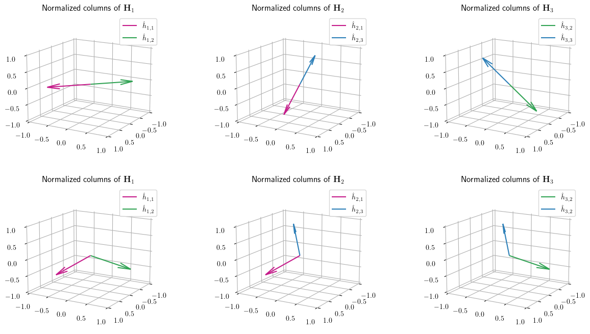
Figure 2: Behavior of locally optimized heads and globally optimized heads.

Appendix C Additional Experimental Results

C.1 Synthetic Datasets

Implementation Details.   In the experiments conducted on synthetic datasets shown in Figure 3, $\mathbf{\Lambda}\in\mathbb{R}^{\underline{d}\times\underline{d}}$ is generated by setting the $i$-th singular value to be $\frac{2\underline{d}}{i+1}$. We randomly generate $\mathbf{U}\in\mathbb{R}^{d\times\underline{d}}$ with $\underline{d}$ orthonormal columns and $\mathbf{V}\in\mathbb{R}^{\underline{d}\times M}$ with $\underline{d}$ orthonormal rows. The ground-truth model is then $\mathbf{\Phi}=\mathbf{U}\mathbf{\Lambda}\mathbf{V}^{\top}$, where each column $\phi_{i}$ represents the local ground-truth model for client $i$. Each client generates $N$ samples $(x,y)$ from $y=x^{\top}\phi_{i}+\xi_{i}$, where $x$ is sampled from a standard Gaussian distribution and every entry of $\xi_{i}$ is IID sampled from $\mathcal{N}(0,0.3)$. The learning rate is set to $\eta=0.03$, and for random initialization, we set $\alpha=\frac{1}{10d}$.

Parameter Settings.   For experiments on synthetic datasets shown in Figure 3, we set $d=10$. We select the value of $k$ from the set $\{2,4,6,8\}$, $M$ from the set $\{15,30\}$, and $N$ from the set $\{12,20\}$.

Experimental Results.   From the experiments in Figure 3, we observe that, with the dimensions $d$, $M$, and $N$ fixed, an increase in $k$ results in a diminishing discrepancy in convergence speeds between FLUTE and FedRep. This trend demonstrates FLUTE’s superior performance in under-parameterized settings. Furthermore, keeping $d$, $k$, and $N$ unchanged while increasing the number of clients $M$, we see a reduction in the average error of models generated by FLUTE. This observation aligns with our theoretical findings presented in Theorem 5.5.

Varying $\gamma_{1}$ and $\gamma_{2}$.   In Figure 4, we report the results of the following experiments where $d=10$, $k=6$, $M=10$, and $N$ selected from the set $\{8,9,10,11\}$. For comparison, we use three pairs of $\gamma_{1}$ and $\gamma_{2}$: $\gamma_{1}=2\gamma_{2}$, $\gamma_{1}=\gamma_{2}$, and $\gamma_{1}=\frac{2}{3}\gamma_{2}$. We do not set $\gamma_{1}>2\gamma_{2}$ because in this setting, $\|\mathbf{B}\mathbf{W}\|_{F}$ usually diverges. From the experimental results, we observe that when $N=8$, $9$, or $10$, $\gamma_{1}=\gamma_{2}$ shows the best performance among the three settings of $\gamma_{1}$ and $\gamma_{2}$.

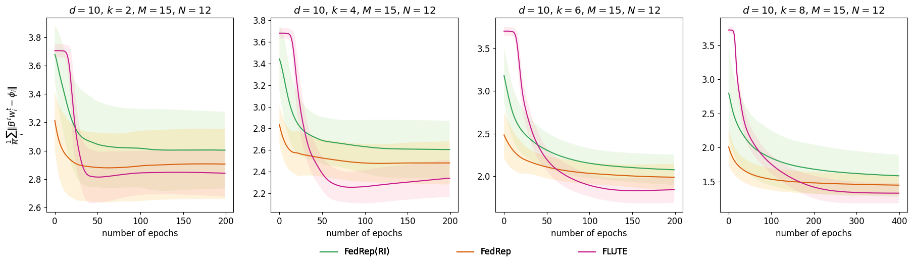
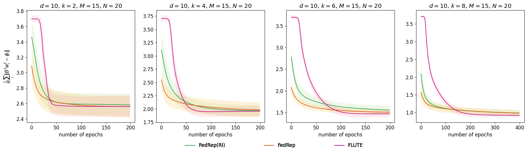
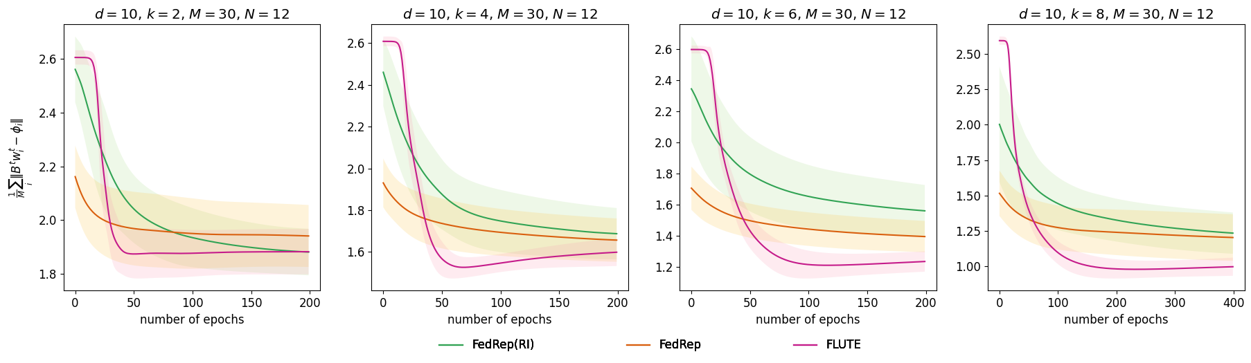
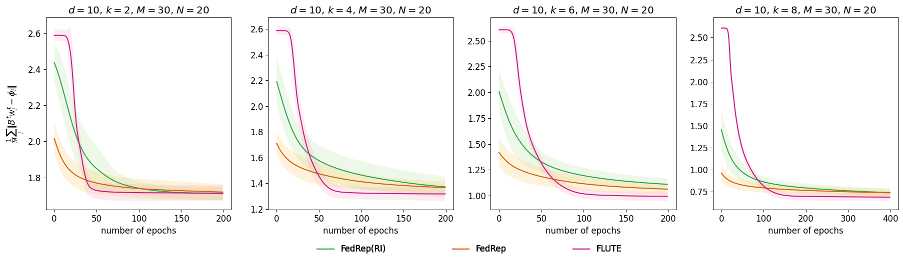
Figure 3: Experimental results with synthetic datasets.

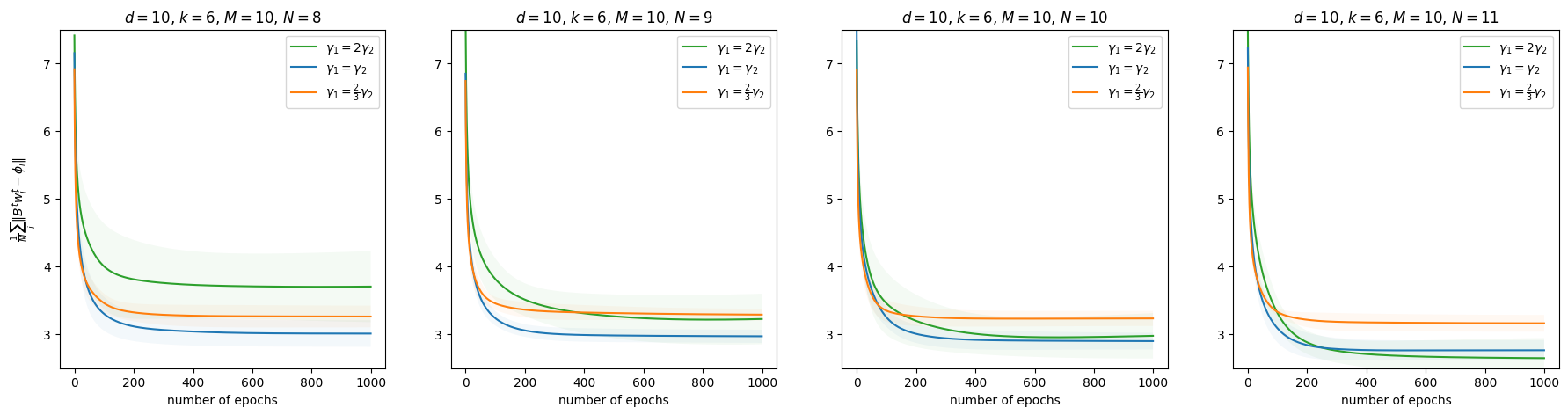
Figure 4: Experimental results with synthetic datasets.

C.2 Real-world Datasets

Implementation Details.   For our experiments on the CIFAR-10 dataset, we employ a 5-layer CNN architecture. It begins with a convolutional layer Conv2d(3, 64, 5), followed by a pooling layer MaxPool2d(2, 2). The second convolutional layer is Conv2d(64, 64, 5), which precedes three fully connected layers: Linear(64*5*5, 120), Linear(120, 64), and Linear(64, 10). In contrast, for the CIFAR-100 dataset, we also use a 5-layer CNN, but with some modifications to accommodate the higher complexity of the dataset. The initial layer is Conv2d(3, 64, 5), followed by pooling and dropout layers: MaxPool2d(2, 2) and nn.Dropout(0.6). The subsequent convolutional layer is Conv2d(64, 128, 5). This is succeeded by three fully connected layers: Linear(128*5*5, 256), Linear(256, 128), and Linear(128, 100).

Experimental Results.   In this section, we plot Figure 5 to Figure 12 to illustrate the detailed convergence behavior of the test accuracy of the trained models reported in Table 1 as a function of the training epochs. We augment the test accuracy results by introducing two different metrics. The first one is Global NC2, which is measured by

$$\frac{1}{M}\sum_{i\in[M]}\left\|\frac{\mathbf{H}^{\top}_{i}\mathbf{H}_{i}}{\|\mathbf{H}^{\top}_{i}\mathbf{H}_{i}\|_{F}}-\frac{1}{\sqrt{m-1}}\mathbf{u}_{i}\mathbf{u}_{i}^{\top}\odot\left(\mathbf{I}_{m}-\frac{1}{m}\mathbf{1}_{m}\mathbf{1}^{\top}_{m}\right)\right\|_{F}.$$

The second one is Averaged Local NC2, referred to as

$$\frac{1}{M}\sum_{i\in[M]}\left\|\frac{\mathbf{H}^{\top}_{i}\mathbf{H}_{i}}{\|\mathbf{H}^{\top}_{i}\mathbf{H}_{i}\|_{F}}-\frac{1}{\sqrt{m^{\prime}-1}}\mathbf{u}_{i}\mathbf{u}_{i}^{\top}\odot\left(\mathbf{I}_{m}-\frac{1}{m^{\prime}}\mathbf{1}_{m}\mathbf{1}^{\top}_{m}\right)\right\|_{F}.$$

These two metrics are inspired by B.3 and B.2, respectively. Global NC2 aims to measure the similarity between the learned models and the optimal under-parameterized global model. In contrast, Averaged Local NC2 assesses the similarity between the learned models and the optimal local models. Note that these two metrics are positively correlated, meaning that when one is small, the other is usually small as well. In some results, such as those shown in Figure 5 and Figure 7, the gaps between FedRep* and FLUTE* in terms of Averaged Local NC2 are significantly larger than those in terms of Global NC2, suggesting that the models learned by FLUTE* are closer to the global optimizer than those learned by FedRep*.

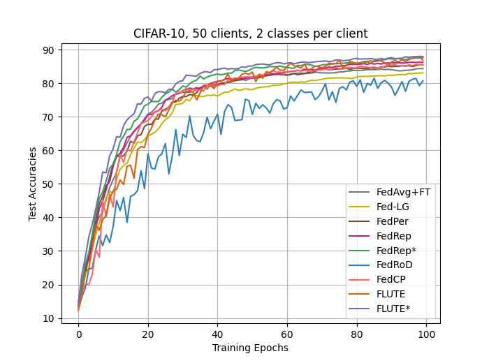
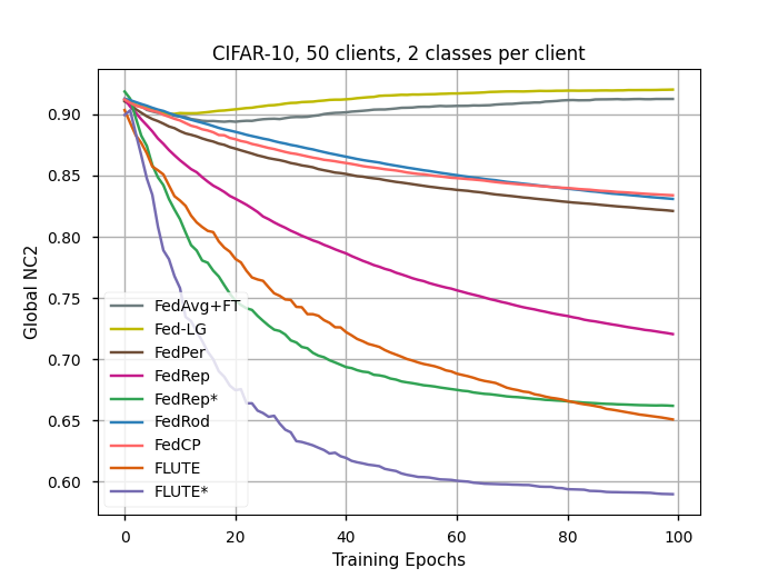
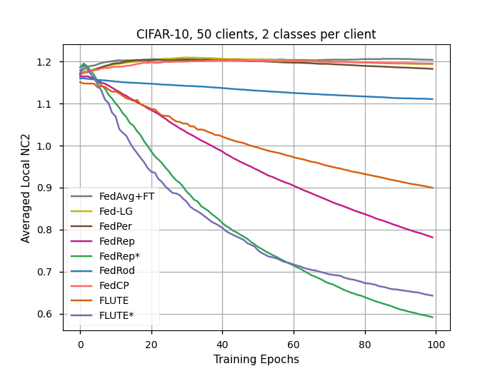
Figure 5: Experimental results for CIFAR10 when $M=50,m^{\prime}=2$.

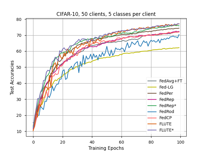
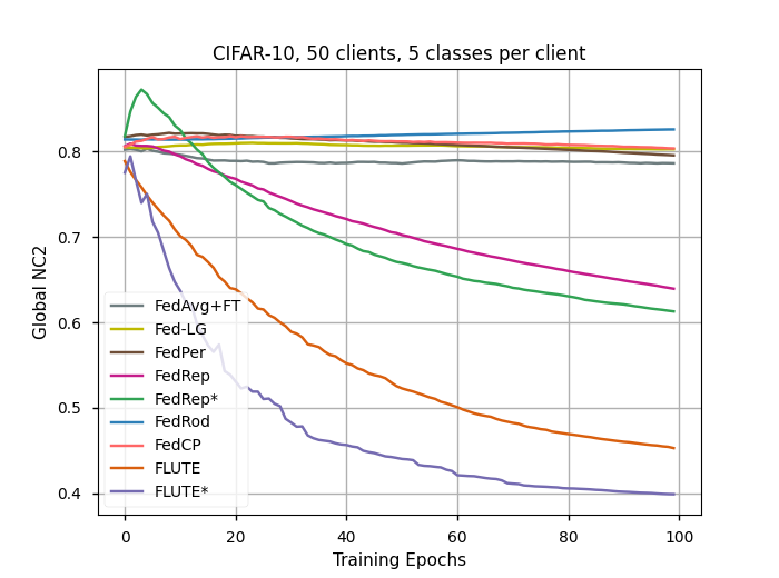
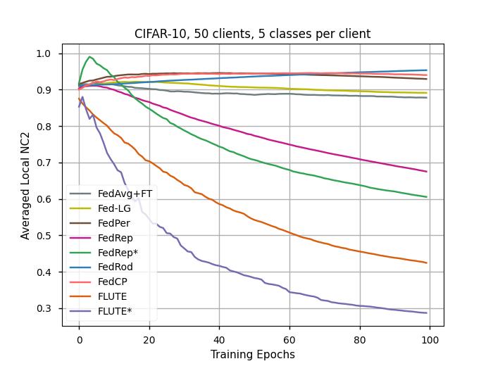
Figure 6: Experimental results for CIFAR10 when $M=50,m^{\prime}=5$.

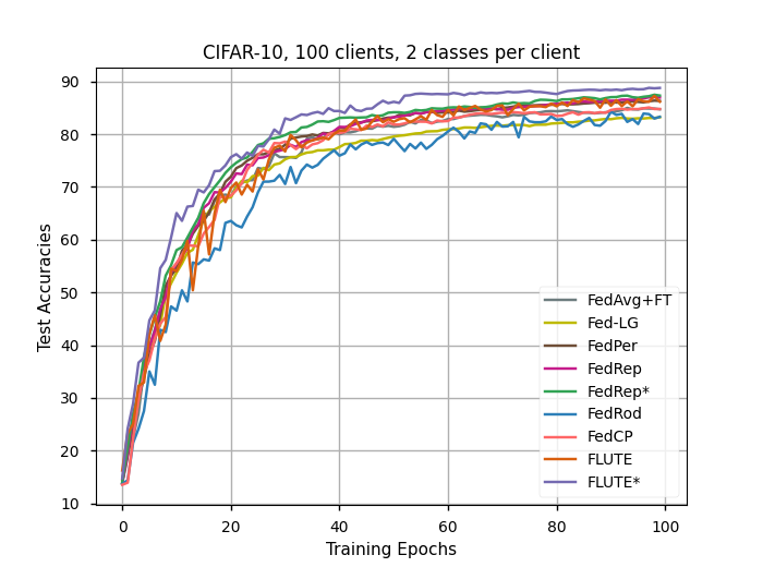
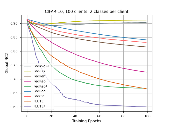
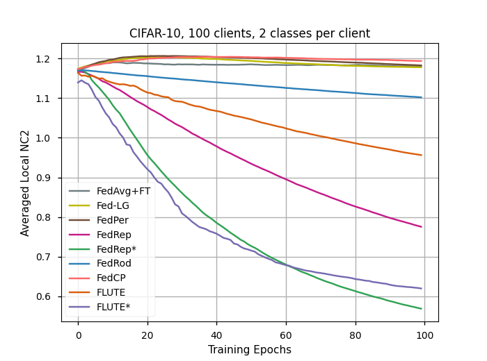
Figure 7: Experimental results for CIFAR10 when $M=100,m^{\prime}=2$.

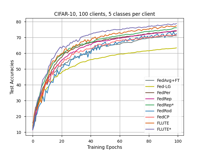
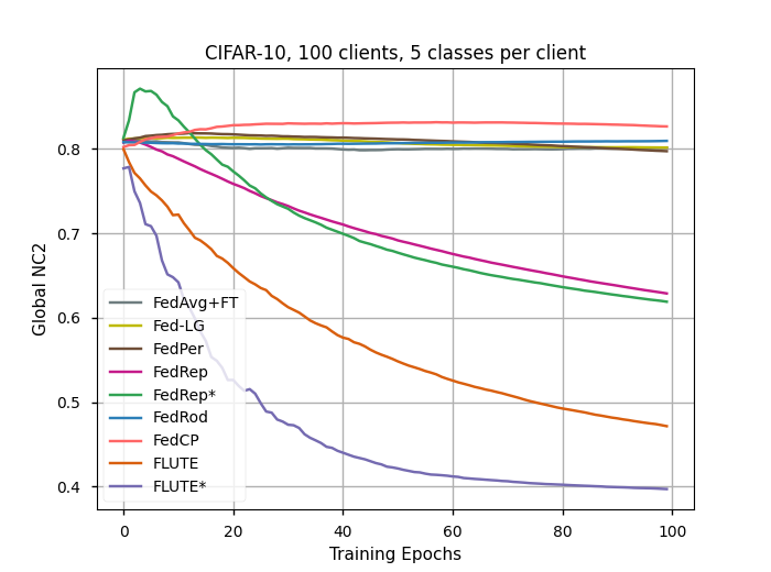
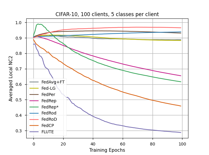
Figure 8: Experimental results for CIFAR10 when $M=50,m^{\prime}=5$.

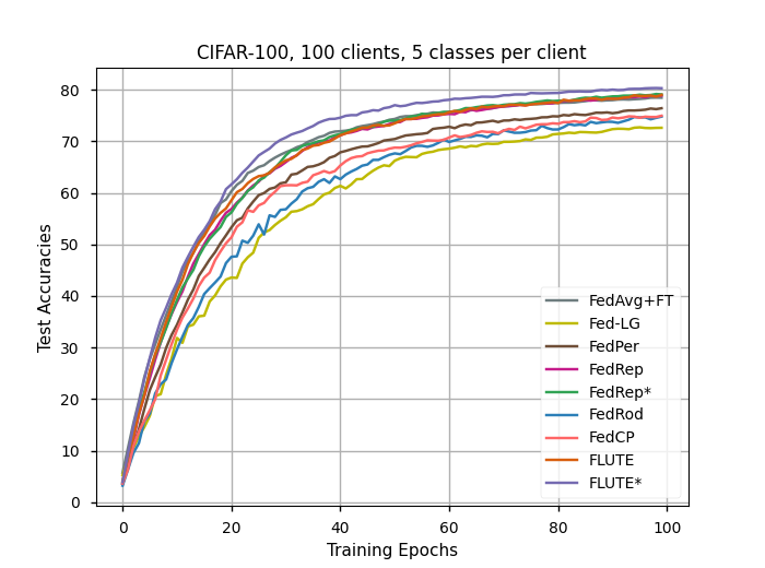
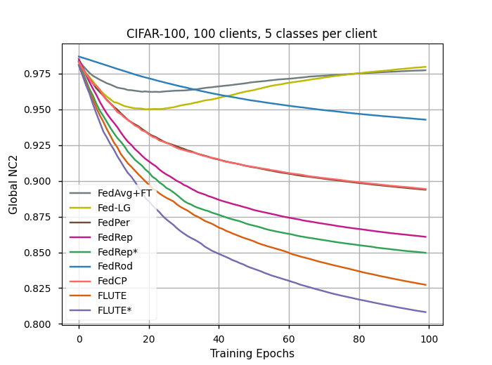
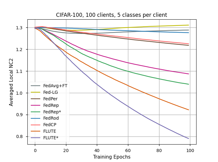
Figure 9: Experimental results for CIFAR100 when $M=100,m^{\prime}=5$.

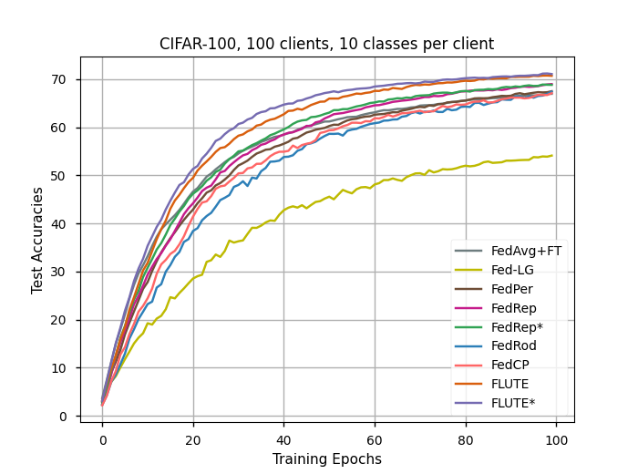
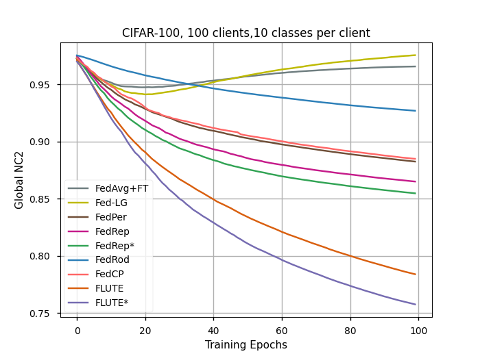
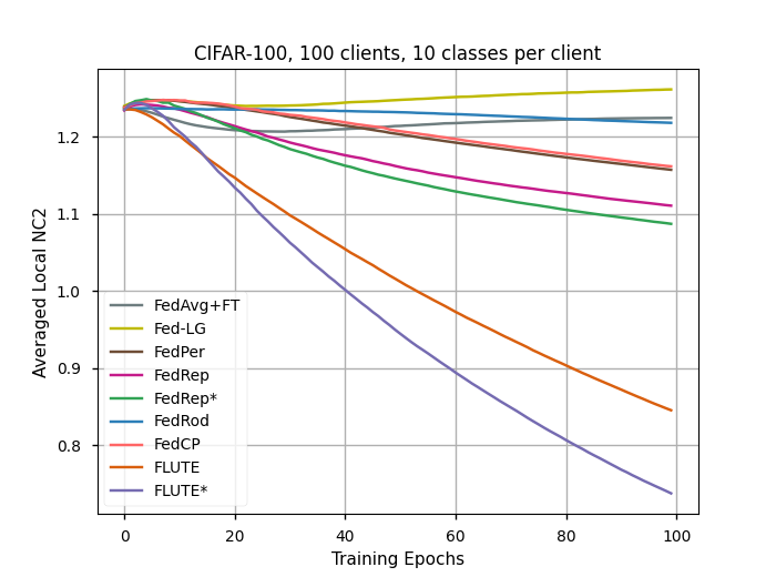
Figure 10: Experimental results for CIFAR100 when $M=100,m^{\prime}=10$.

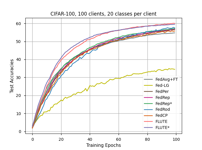
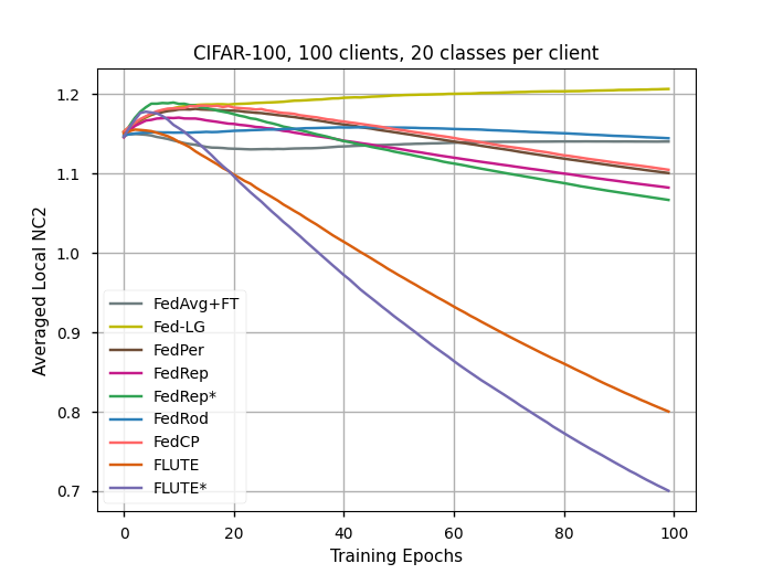
Figure 11: Experimental results for CIFAR100 when $M=100,m^{\prime}=20$.

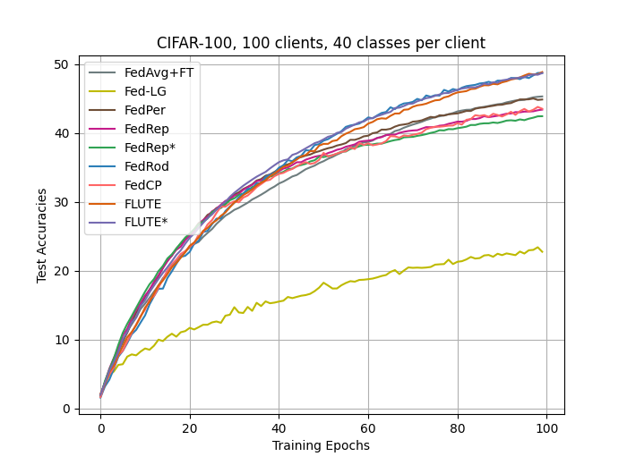
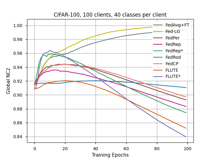
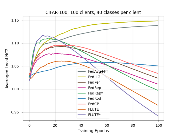
Figure 12: Experimental results for CIFAR100 when $M=100,m^{\prime}=40$.

References

• Arivazhagan et al. (2019) Arivazhagan, M. G., Aggarwal, V., Singh, A. K., and Choudhary, S. Federated learning with personalization layers. arXiv preprint arXiv:1912.00818, 2019.
• Belkin et al. (2019) Belkin, M., Hsu, D., Ma, S., and Mandal, S. Reconciling modern machine-learning practice and the classical bias–variance trade-off. Proceedings of the National Academy of Sciences, 116(32):15849––15854, July 2019.
• Chen et al. (2023) Chen, H., Chen, X., Elmasri, M., and Sun, Q. Fast global convergence of gradient descent for low-rank matrix approximation. arXiv preprint arXiv:2305.19206, 2023.
• Chen & Chao (2021) Chen, H.-Y. and Chao, W.-L. On bridging generic and personalized federated learning for image classification. arXiv preprint arXiv:2107.00778, 2021.
• Chen et al. (2021) Chen, L., Lin, S., Lu, X., Cao, D., Wu, H., Guo, C., Liu, C., and Wang, F.-Y. Deep neural network based vehicle and pedestrian detection for autonomous driving: A survey. IEEE Transactions on Intelligent Transportation Systems, 22(6):3234–3246, 2021.
• Chen et al. (2022) Chen, Y., Dai, X., Chen, D., Liu, M., Dong, X., Yuan, L., and Liu, Z. Mobile-Former: Bridging MobileNet and transformer. In Proceedings of the IEEE/CVF Conference on Computer Vision and Pattern Recognition, pp.  5270–5279, 2022.
• Collins et al. (2021) Collins, L., Hassani, H., Mokhtari, A., and Shakkottai, S. Exploiting shared representations for personalized federated learning. In International Conference on Machine Learning, pp.  2089–2099. PMLR, 2021.
• Davidson & Szarek (2001) Davidson, K. R. and Szarek, S. J. Local operator theory, random matrices and banach spaces. Handbook of the geometry of Banach spaces, 1(317-366):131, 2001.
• Du et al. (2020) Du, S. S., Hu, W., Kakade, S. M., Lee, J. D., and Lei, Q. Few-shot learning via learning the representation, provably. arXiv preprint arXiv:2002.09434, 2020.
• Duchi et al. (2022) Duchi, J., Feldman, V., Hu, L., and Talwar, K. Subspace recovery from heterogeneous data with non-isotropic noise, 2022.
• Finn et al. (2017) Finn, C., Abbeel, P., and Levine, S. Model-agnostic meta-learning for fast adaptation of deep networks. In International Conference on Machine Learning, pp.  1126–1135. PMLR, 2017.
• Ge et al. (2017) Ge, R., Jin, C., and Zheng, Y. No spurious local minima in nonconvex low rank problems: A unified geometric analysis, 2017.
• Golub & Van Loan (2013) Golub, G. H. and Van Loan, C. F. Matrix computations. JHU Press, 2013.
• He et al. (2020) He, C., Annavaram, M., and Avestimehr, S. Group knowledge transfer: Federated learning of large CNNs at the edge. Advances in Neural Information Processing Systems, 33:14068–14080, 2020.
• He et al. (2016) He, K., Zhang, X., Ren, S., and Sun, J. Deep residual learning for image recognition. In Proceedings of the IEEE Conference on Computer Vision and Pattern Recognition, pp.  770–778, 2016.
• Hitaj et al. (2017) Hitaj, B., Ateniese, G., and Perez-Cruz, F. Deep models under the gan: information leakage from collaborative deep learning. In Proceedings of the 2017 ACM SIGSAC Conference on Computer and Communications Security, pp.  603–618, 2017.
• Howard et al. (2019) Howard, A., Sandler, M., Chu, G., Chen, L.-C., Chen, B., Tan, M., Wang, W., Zhu, Y., Pang, R., Vasudevan, V., et al. Searching for mobilenetv3. In Proceedings of the IEEE/CVF International Conference on Computer Vision, pp.  1314–1324, 2019.
• Hsu et al. (2012) Hsu, D., Kakade, S. M., and Zhang, T. Random design analysis of ridge regression. In Conference on Learning Theory, pp.  9–1. JMLR Workshop and Conference Proceedings, 2012.
• Hwang (2004) Hwang, S.-G. Cauchy’s interlace theorem for eigenvalues of hermitian matrices. The American Mathematical Monthly, 111(2):157–159, 2004.
• Jiang et al. (2022) Jiang, L., Chen, Y., and Ding, L. Algorithmic regularization in model-free overparametrized asymmetric matrix factorization. arXiv preprint arXiv:2203.02839, 2022.
• Ju et al. (2023) Ju, R.-Y., Lin, T.-Y., Jian, J.-H., and Chiang, J.-S. Efficient convolutional neural networks on Raspberry Pi for image classification. Journal of Real-Time Image Processing, 20(2):21, 2023.
• Kairouz et al. (2021) Kairouz, P., McMahan, H. B., Avent, B., Bellet, A., Bennis, M., Bhagoji, A. N., Bonawitz, K., Charles, Z., Cormode, G., Cummings, R., et al. Advances and open problems in federated learning. Foundations and Trends® in Machine Learning, 14(1–2):1–210, 2021.
• Krizhevsky et al. (2009) Krizhevsky, A., Hinton, G., et al. Learning multiple layers of features from tiny images. 2009.
• LeCun et al. (2015) LeCun, Y., Bengio, Y., and Hinton, G. Deep learning. Nature, 521(7553):436–444, 2015.
• Li et al. (2020) Li, T., Sahu, A. K., Talwalkar, A., and Smith, V. Federated learning: Challenges, methods, and future directions. IEEE Signal Processing Magazine, 37(3):50–60, 2020.
• Liang et al. (2020) Liang, P. P., Liu, T., Ziyin, L., Allen, N. B., Auerbach, R. P., Brent, D., Salakhutdinov, R., and Morency, L.-P. Think locally, act globally: Federated learning with local and global representations. arXiv preprint arXiv:2001.01523, 2020.
• Liu et al. (2017) Liu, W., Wang, Z., Liu, X., Zeng, N., Liu, Y., and Alsaadi, F. E. A survey of deep neural network architectures and their applications. Neurocomputing, 234:11–26, 2017.
• McMahan et al. (2017) McMahan, B., Moore, E., Ramage, D., Hampson, S., and y Arcas, B. A. Communication-efficient learning of deep networks from decentralized data. In AISTATS, pp.  1273–1282. PMLR, 2017.
• Melis et al. (2019) Melis, L., Song, C., De Cristofaro, E., and Shmatikov, V. Exploiting unintended feature leakage in collaborative learning. In 2019 IEEE Symposium on Security and Privacy (SP), pp.  691–706, 2019.
• Mitra et al. (2021) Mitra, A., Jaafar, R., Pappas, G. J., and Hassani, H. Linear convergence in federated learning: Tackling client heterogeneity and sparse gradients. Advances in Neural Information Processing Systems, 34:14606–14619, 2021.
• Oneto et al. (2023) Oneto, L., Ridella, S., and Anguita, D. Do we really need a new theory to understand over-parameterization? Neurocomputing, 543:126227, 2023.
• OpenAI (2023) OpenAI. Gpt-4 technical report, 2023.
• Papyan et al. (2020) Papyan, V., Han, X. Y., and Donoho, D. L. Prevalence of neural collapse during the terminal phase of deep learning training. Proceedings of the National Academy of Sciences, 117(40):24652–24663, Sept. 2020.
• Pitaval et al. (2015) Pitaval, R.-A., Dai, W., and Tirkkonen, O. Convergence of gradient descent for low-rank matrix approximation. IEEE Transactions on Information Theory, 61(8):4451–4457, 2015.
• Rudelson & Vershynin (2008) Rudelson, M. and Vershynin, R. The littlewood-offord problem and invertibility of random matrices, 2008.
• Shen et al. (2023) Shen, Z., Ye, J., Kang, A., Hassani, H., and Shokri, R. Share your representation only: Guaranteed improvement of the privacy-utility tradeoff in federated learning, 2023.
• Tan et al. (2022) Tan, J., Mason, B., Javadi, H., and Baraniuk, R. Parameters or privacy: A provable tradeoff between overparameterization and membership inference. Advances in Neural Information Processing Systems, 35:17488–17500, 2022.
• Tan & Le (2019) Tan, M. and Le, Q. Efficientnet: Rethinking model scaling for convolutional neural networks. In International Conference on Machine Learning, pp.  6105–6114. PMLR, 2019.
• Thekumparampil et al. (2021) Thekumparampil, K. K., Jain, P., Netrapalli, P., and Oh, S. Sample efficient linear meta-learning by alternating minimization, 2021.
• Tirer & Bruna (2022) Tirer, T. and Bruna, J. Extended unconstrained features model for exploring deep neural collapse, 2022.
• Touvron et al. (2023) Touvron, H., Lavril, T., Izacard, G., Martinet, X., Lachaux, M.-A., Lacroix, T., Rozière, B., Goyal, N., Hambro, E., Azhar, F., Rodriguez, A., Joulin, A., Grave, E., and Lample, G. Llama: Open and efficient foundation language models, 2023.
• Tripuraneni et al. (2021) Tripuraneni, N., Jin, C., and Jordan, M. Provable meta-learning of linear representations. In International Conference on Machine Learning, pp.  10434–10443. PMLR, 2021.
• Vershynin (2010) Vershynin, R. Introduction to the non-asymptotic analysis of random matrices. arXiv preprint arXiv:1011.3027, 2010.
• Wang et al. (2016a) Wang, J., Kolar, M., and Srebro, N. Distributed multi-task learning with shared representation. arXiv preprint arXiv:1603.02185, 2016a.
• Wang et al. (2016b) Wang, L., Zhang, X., and Gu, Q. A unified computational and statistical framework for nonconvex low-rank matrix estimation, 2016b.
• Wang et al. (2019) Wang, S., Tuor, T., Salonidis, T., Leung, K. K., Makaya, C., He, T., and Chan, K. Adaptive federated learning in resource constrained edge computing systems. IEEE Journal on Selected Areas in Communications, 37(6):1205–1221, 2019.
• Wang et al. (2018) Wang, Z., Song, M., Zhang, Z., Song, Y., Wang, Q., and Qi, H. Beyond inferring class representatives: User-level privacy leakage from federated learning, 2018.
• Ye & Du (2021) Ye, T. and Du, S. S. Global convergence of gradient descent for asymmetric low-rank matrix factorization, 2021.
• Yu et al. (2020) Yu, T., Bagdasaryan, E., and Shmatikov, V. Salvaging federated learning by local adaptation. arXiv preprint arXiv:2002.04758, 2020.
• Zhang et al. (2023a) Zhang, J., Hua, Y., Wang, H., Song, T., Xue, Z., Ma, R., and Guan, H. Fedcp: Separating feature information for personalized federated learning via conditional policy. In Proceedings of the 29th ACM SIGKDD Conference on Knowledge Discovery and Data Mining, pp.  3249–3261, 2023a.
• Zhang et al. (2023b) Zhang, T. T. C. K., Toso, L. F., Anderson, J., and Matni, N. Meta-learning operators to optimality from multi-task non-iid data, 2023b.
• Zhong et al. (2022) Zhong, A., He, H., Ren, Z., Li, N., and Li, Q. Feddar: Federated domain-aware representation learning. arXiv preprint arXiv:2209.04007, 2022.
• Zhu et al. (2021a) Zhu, Z., Ding, T., Zhou, J., Li, X., You, C., Sulam, J., and Qu, Q. A geometric analysis of neural collapse with unconstrained features, 2021a.
• Zhu et al. (2021b) Zhu, Z., Li, Q., Tang, G., and Wakin, M. B. The global optimization geometry of low-rank matrix optimization, 2021b.