[a,b]Shoji Hashimoto
Towards understanding of the inclusive vs exclusive puzzle in the determinations
Abstract
Lattice calculation may play an important role to understand the cause of the long-standing puzzle among the determination of . The key element is the computation of the inclusive decay rate, for which the formalism is under development. The method has its own problem: the approximation of the phase-space factor and finite volume effect. I discuss the current status of such study and future prospects.
1 The puzzle
It has been more than a decade since the tension between the exclusive and inclusive determinations of and is recognized (see [1] for a review). Other than various experimental issues, the exclusive method relies on the lattice QCD calculation of the relevant form factors such as or , for which some potential problems are discussed in a companion talk [2], while the inclusive determination uses the perturbative QCD method supplemented by the operator product expansion (OPE) to calculate the semi-leptonic decay rate at the quark level, which corresponds to the sum over all possible final states. In OPE, one needs matrix elements of the operators sandwiched by the initial meson states; they can be determined in principle by fitting the experimental data of the integrated decay rate with various kinematical cuts. Theoretically, both the exclusive and inclusive methods are considered reliable and systematically improvable, so that the tension poses a tremendous challenge for the theorists (assuming that the systematic uncertainties in the experimental analysis is reliable).
Ideally, the puzzle can be solved if the decay rate was obtained both experimentally and theoretically in the entire phase space of the semi-leptonic decays, i.e. the invariant mass of the final hadronic state and its recoil momentum (apart from the angular distributions), and if the determinations of at each point of the phase space all agreed. But, theoretically the calculation of the differential decay rate is a formidable task even with the first-principles simulation of lattice QCD, especially for excited hadronic final states. More tractable is a non-perturbative lattice calculation of the integrated decay rate over some phase space, and it is the subject of this talk. The integral over the phase space reduces to the inclusive rate when the entire phase space is covered. There are many other observables such as those with kinematical cuts or some moments of and so on.
In the following sections, I briefly outline the formalism to compute such integrated rates in lattice QCD. Then, some discussions of potential systematic errors and future prospects follow.
2 Formalism for the inclusive rate
The differential rate of semi-leptonic decays can be written as using the structure function (or hadronic tensor) :
| (1) |
where the sum runs over all possible hadronic final states with momentum [3, 4]. The flavor-changing current induces the weak decay, and the momentum is transferred to the lepton pair and . The leptonic tensor is a known kinematical factor. Since the structure function is expressed as an imaginary part of the matrix element (sometimes called the Compton amplitude)
| (2) |
of a product of currents , one can use OPE to approximate by a series of local operators, such as , , , and so on. It leads to an expansion in terms of inverse quark mass , since the momentum flowing into the charm quark propagator is of order of . This forms a basis of the perturbative estimates of the inclusive decay rate. The matrix elements of the local operators sandwiched by the meson states could be determined by fitting the experimental data of various quantities. Some examples are shown, for instance, in [5], where the lepton energy and hadronic invariant mass moments are fitted against the lepton energy cut applied in the experimental analysis. Recent inclusive analysis includes the perturbative expansion to the order of and the heavy quark expansion to (see, for instance, [6]).
Another important problem in the semi-leptonic meson decays is the “missing component” of the fully inclusive rate. Namely, the sum of known exclusive decays such as , , etc. is less than the measurement of the total inclusive rate by about 15%. (See Table XIV of [1].) This needs to be understood within the experimental analysis, but theoretical information about the decay form factors to excited state mesons would also be helpful. Some discussions are found in the companion talk [2].
Concerning the “inclusive versus exclusive puzzle”, there is also a theoretical question about the validity of the quark-hadron duality. Since the inclusive decays are dominated by the -wave states and to about 2/3 of the total decay rate, there is not so much room left for the excited states. The duality is expected to work only when the hadronic states are sufficiently smeared, or summed, so that the details of the bound-state dynamics become irrelevant. Quantitative estimate of the duality violation effect is, however, very difficult.
3 Formalism for the lattice calculation
On the lattice one can compute matrix elements of some operators. For the calculation of semi-leptonic decay form factors of exclusive processes, the matrix element of the form is computed. Similarly the Compton amplitude (2) can be computed on the Euclidean lattice, but it corresponds to an unphysical kinematical setup. For example, the hadronic energy accessible from the Fourier transform of the Euclidean lattice data does not correspond to the physical states; a strategy to connect the lattice data to some physical observables was proposed in [7], but the following method allows more direct calculation of experimentally measured quantities.
An alternative approach is to view the Compton amplitude (2) as a spectral function. One can write the integrand of the matrix element as
| (3) |
for a given energy . The currents are Fourier transformed to the momentum space; the temporal direction remains in the coordinate space and the energy is specified by the with the QCD Hamiltonian . The inclusive rate can then be expressed as an integral of (3) over and with a weight factor (or a kernel function ) determined by the kinematical factor. Once this type of the spectral function was extracted from the lattice calculation, one can perform the integral over and , but the extraction of the spectral function from the Euclidean lattice calculation is known as a ill-posed inverse problem and only some approximate numerical solution can be obtained [8].
A concrete proposal to bypass this problem is given in [9]. One realizes that the integral over the energy appearing in the expression of the decay rate can be expressed as
| (4) |
On the other hand, the Euclidean correlation function calculated on the lattice yields
| (5) |
Therefore, if there is an approximation of the form
| (6) |
one can relate the integrated decay rate and the lattice correlators. Each term of the right hand side corresponds to the correlator of a fixed time separation between the two current insertions.
The approximation of the form (6) can be implemented in various ways. Essentially, the kernel can be considered as a kind of smearing of the spectral function, as can be seen in (4), a weighted integral over . Solving the spectral function is an ill-posed problem, but once it is smeared over some energy range, it may become much easier. The form of the smearing cannot be controlled in the original form of the Backus-Gilbert method [8], but it was realized that the smearing can be specified by including as a minimization in the Backus-Gilbert method [10]. Another class of the approximation using an orthogonal polynomial method was also proposed [11]. We mainly discuss on this Chebyshev polynomial method in the following.
4 Kernel approximation
The kernel to be approximated has the following form:
| (7) |
Here, the factor is introduced to keep a non-zero time separation between the two currents. The configuration of having two currents in the equal Euclidean time reflects the contributions from both and , each of which corresponds to different kinematical regions; to obtain the semi-leptonic decays one has to restrict in . The next factor comes from the leptonic tensor and = 0, 1 or 2. The Heaviside function is introduced to implement the kinematical upper limit of the integral. The lower limit can be set to zero or to any value below the energy of the lowest hadronic state.
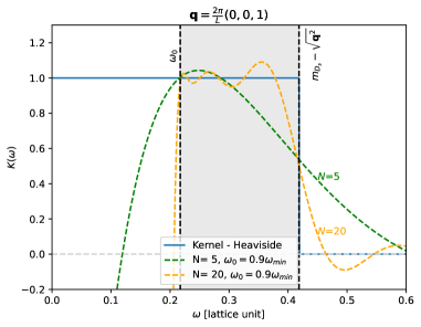
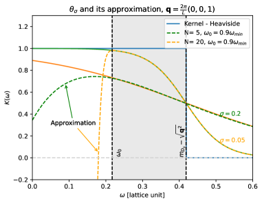
An example of the kernel function and its approximation are shown in Fig. 1. For clarity, we take the Heaviside function as a kernel and ignore the factor and set . The kernel function has a discontinuity at the kinematical upper limit (Fig. 1); we introduce a smoothing (or smearing) to ease the polynomial approximation by replacing the Heaviside function by a sigmoid function . The parameter represents the width of the smearing. In the end, we have to take the limit .
The Chebyshev approximation is one of orthogonal polynomial expansions. (For the definitions and various physics applications, see [12].) In our case, it is written as
| (8) |
where is the Chebyshev polynomial defined in the range . (In practice, we use the shifted Chebyshev polynomial so that is defined in .) The kernel operator is sandwiched by the meson state , and it is evaluated with the operators on the right hand side appearing by expansing the Chebyshev polynomials. Each term simply corresponds the (integer) time separation between the two currents.
The expansion in (8) is mathematically well-defined as forms a orthogonal basis; the coefficients can be easily calculated once the kernel function is given. Moreover, the expansion is known to give the “best” approximation in the sense that the maximum deviation in the range is minimal for a given order .
One important property of the Chebyshev polynomials is that the value is confined in the region . It then leads to a constraint , that comes from an obvious condition for the Hamiltonian eigenvalues. Combining with the expansion (8), this constraint gives a strict upper- and lower-limits of the estimate by taking as two extreme cases for the ignored terms . The systematic error due to the approximation can thus be estimated strictly as . (Remember that the ’s are calculated at low cost, and typically dumps exponentially for large .) This is an advantage over other methods such as that of [10].
5 Early calculations
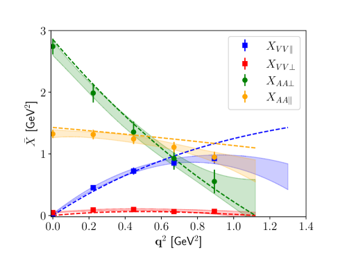
An early result for the differential decay rate (divided by ) from [9, 14] is shown in (2). Here the initial quark is lighter than its physical value (about 3 GeV), so that the kinematical upper-limit for is also made lower. The results for different channels are plotted separately as a function of the recoil momentum squared . The channels are those of vector or axial-vector current insertions, and of different orientation of the currents (parallel or perpendicular to ).
Also plotted by the dashed line is the expectation from the ground state (the -wave and mesons) contributions. They are obtained from the form factor calculations associated with the work [15, 16]. It turned out that the inclusive rate is saturated by the ground states, as anticipated due to the smaller phase-space compared to the physical setup because of the smaller -quark mass. By inspecting the individual matrix elements , we can identify the excited-state contributions, but their size is insignificant at the scale of this plot.
The results are compared with OPE in [14], where the perturbative calculation is performed to and the power corrections are included to . They are in good agreement, although the systematic error of the OPE calculation is large because the lattice calculation is done at smaller quark mass, where the power corrections are enhanced.
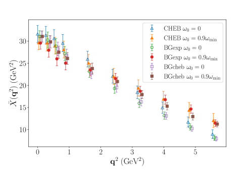
First calculation at the physical quark mass is performed by [17]. In Fig. 3 the differential decay rate (divided by ) is plotted for different choices of the kernel approximations, basically the Chebyshev approximation and Backus-Gilbert method. The results are in good agreement among the methods. Indeed, we confirmed that the resulting approximation curve of the kernel function is very similar between Chebyshev and Backus-Gilbert. A slight deviation among different setup is visible at large values of depending on the choice of , the lower limit of the approximation. It suggests that there is still some hidden uncertainty in the kernel approximation.
6 Systematic errors
This brings us to more detailed study of the systematic errors. In particular, the largest momentum point of in Fig. 2 (the blue point around = 0.9 GeV2) may suggest a problem: the inclusive rate is significantly lower than the ground state ( meson) contribution.
The same channel, but for the meson decays, is studied in [13]. Near the maximum the kernel function has a narrow support from the lowest energy state up to the upper limit . (The kinematical endpoint is defined by the limit where the lowest and the upper limit meet.) As one can imagine from Fig. 1 the kernel approximation gets harder in this limit. Roughly speaking, the polynomial of order allows the slope of the approximated kernel of about , which corresponds to the Heaviside-like change within the range of . When the support of the kernel becomes as small as this width, the approximation would become imprecise.
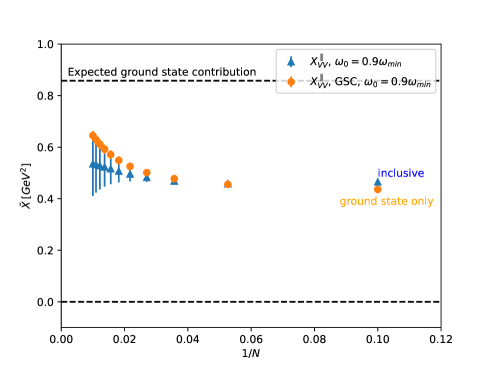
In order to control such systematic effect, we introduce a smeared Heaviside function with a width and set it to . Then, the Chebyshev approximation at the order follow the smeared kernel rather precisely. Even though the lattice data are not available for large time separation, thus large , one can obtain the upper and lower limit of the estimate for arbitrary by setting their Chebyshev matrix elements of unknown higher orders to as mentioned above. It is done in Fig. 4, and the estimate is shown as a function of . Towards the limit of , one can see that the error increases for the (differential) inclusive rate. Also plotted is its contribution from the ground state, for which the energy is precisely known and the distortion due to the kernel approximation can be traced. We find that the inclusive rate actually covers the ground-state contribution for each value of ; the limit of may be estimated by an extrapolation. One may think that the error in the limit is too large to be useful, but one can avoid the problem for this particular case because we know that the ground state saturates the decay rate.
Another potentially important source of the systematic error is the finite volume effect. The excited states consist of multi-hadron final states, and their spectrum becomes discrete in a finite box and a systematic error of is expected. The size of such error can be estimated by assuming the two-body spectrum and their amplitude [18].
7 Final remarks: towards understanding the puzzle
As outline above, there is a formulation to compute the inclusive decay rate using lattice QCD. It doesn’t require the reconstruction of the spectral function, and one can avoid the ill-posed inverse problem. The new method involves new problems, though. The kernel approximation is challenging when the hard energy cutoff has to be implemented like the case of the inclusive decay rate. A good news is that the systematic error can be rigorously estimated with the Chebyshev polynomial method.
Some initial lattice studies are encouraging. Comparison with the OPE-based approach has been made; the study should be extended to the calculations with the physical kinematics. Such consistency check would finally establish the consistency among the theories of inclusive decays, i.e. OPE and lattice. Eventually, the comparison should also be made for various moments, such as those of lepton energy and hadronic mass. Lattice calculation of them can be performed in parallel with the decay rate.
More detailed comparison among the OPE, lattice and experiments are possible. In addition to the total decay rate and moments, one can consider any weighted integrals of the differential decay rate. Each party (OPE, lattice, experiment) has its own advantages and weaknesses, and one can reach the optimal solution after compromises. For instance, the lattice calculation is harder and thus less precise for large recoil momenta, while the experiment is not able to cover too small momenta. The OPE method needs a sufficiently broad range of integral to avoid potential problems due to the quark-hadron duality. Close collaborations among different parties would be crucial to finally resolve the puzzle.
I thank the present and past members of the JLQCD collaboration, as well as other collaborators that led to the publications [14, 17]. A lot of materials in this presentation emerged from the discussions with them.
This work is partly supported by MEXT as “Program for Promoting Researches on the Supercomputer Fugaku” (JPMXP1020200105) and by JSPS KAKENHI, Grant-Number 22H00138. This work used computational resources of supercomputer Fugaku provided by the RIKEN Center for Computational Science through the HPCI System Research Projects (Project IDs: hp120281, hp230245), SX-Aurora TSUBASA at the High Energy Accelerator Research Organization (KEK) under its Particle, Nuclear and Astrophysics Simulation Program (Project IDs: 2019L003, 2020-006, 2021-007, 2022-006 and 2023-004).
References
- [1] J. Dingfelder and T. Mannel, Rev. Mod. Phys. 88 (2016) no.3, 035008 doi:10.1103/RevModPhys.88.035008
- [2] S. Hashimoto, “Next challenges in semi-leptonic decays,” PoS(EuroPLEx2023) 013; a talk at the EuroPLEx2023 workshop.
- [3] B. Blok, L. Koyrakh, M. A. Shifman and A. I. Vainshtein, Phys. Rev. D 49 (1994), 3356 [erratum: Phys. Rev. D 50 (1994), 3572] doi:10.1103/PhysRevD.50.3572 [arXiv:hep-ph/9307247 [hep-ph]].
- [4] A. V. Manohar and M. B. Wise, Phys. Rev. D 49 (1994), 1310-1329 doi:10.1103/PhysRevD.49.1310 [arXiv:hep-ph/9308246 [hep-ph]].
- [5] P. Gambino and C. Schwanda, Phys. Rev. D 89 (2014) no.1, 014022 doi:10.1103/PhysRevD.89.014022 [arXiv:1307.4551 [hep-ph]].
- [6] T. Mannel and A. A. Pivovarov, Phys. Rev. D 100 (2019) no.9, 093001 doi:10.1103/PhysRevD.100.093001 [arXiv:1907.09187 [hep-ph]].
- [7] S. Hashimoto, PTEP 2017 (2017) no.5, 053B03 doi:10.1093/ptep/ptx052 [arXiv:1703.01881 [hep-lat]].
- [8] M. T. Hansen, H. B. Meyer and D. Robaina, Phys. Rev. D 96 (2017) no.9, 094513 doi:10.1103/PhysRevD.96.094513 [arXiv:1704.08993 [hep-lat]].
- [9] P. Gambino and S. Hashimoto, Phys. Rev. Lett. 125 (2020) no.3, 032001 doi:10.1103/PhysRevLett.125.032001 [arXiv:2005.13730 [hep-lat]].
- [10] M. Hansen, A. Lupo and N. Tantalo, Phys. Rev. D 99 (2019) no.9, 094508 doi:10.1103/PhysRevD.99.094508 [arXiv:1903.06476 [hep-lat]].
- [11] G. Bailas, S. Hashimoto and T. Ishikawa, PTEP 2020 (2020) no.4, 043B07 doi:10.1093/ptep/ptaa044 [arXiv:2001.11779 [hep-lat]].
- [12] A. Weisse, G. Wellein, A. Alvermann and H. Fehske, Rev. Mod. Phys. 78 (2006), 275-306 doi:10.1103/RevModPhys.78.275 [arXiv:cond-mat/0504627 [cond-mat.other]].
- [13] R. Kellermann, A. Barone, S. Hashimoto, A. Jüttner and T. Kaneko, PoS LATTICE2022 (2023), 414 doi:10.22323/1.430.0414 [arXiv:2211.16830 [hep-lat]].
- [14] P. Gambino, S. Hashimoto, S. Mächler, M. Panero, F. Sanfilippo, S. Simula, A. Smecca and N. Tantalo, JHEP 07 (2022), 083 doi:10.1007/JHEP07(2022)083 [arXiv:2203.11762 [hep-lat]].
- [15] B. Colquhoun et al. [JLQCD], Phys. Rev. D 106 (2022) no.5, 054502 doi:10.1103/PhysRevD.106.054502 [arXiv:2203.04938 [hep-lat]].
- [16] Y. Aoki et al. [JLQCD], Phys. Rev. D 109 (2024) no.7, 074503 doi:10.1103/PhysRevD.109.074503 [arXiv:2306.05657 [hep-lat]].
- [17] A. Barone, S. Hashimoto, A. Jüttner, T. Kaneko and R. Kellermann, JHEP 07 (2023), 145 doi:10.1007/JHEP07(2023)145 [arXiv:2305.14092 [hep-lat]].
- [18] R. Kellermann, A. Barone, S. Hashimoto, A. Jüttner and T. Kaneko, PoS LATTICE2023 (2024), 272 doi:10.22323/1.453.0272 [arXiv:2312.16442 [hep-lat]].