On the Expressive Power of Spectral Invariant Graph Neural Networks
Abstract
Incorporating spectral information to enhance Graph Neural Networks (GNNs) has shown promising results but raises a fundamental challenge due to the inherent ambiguity of eigenvectors. Various architectures have been proposed to address this ambiguity, referred to as spectral invariant architectures. Notable examples include GNNs and Graph Transformers that use spectral distances, spectral projection matrices, or other invariant spectral features. However, the potential expressive power of these spectral invariant architectures remains largely unclear. The goal of this work is to gain a deep theoretical understanding of the expressive power obtainable when using spectral features. We first introduce a unified message-passing framework for designing spectral invariant GNNs, called Eigenspace Projection GNN (EPNN). A comprehensive analysis shows that EPNN essentially unifies all prior spectral invariant architectures, in that they are either strictly less expressive or equivalent to EPNN. A fine-grained expressiveness hierarchy among different architectures is also established. On the other hand, we prove that EPNN itself is bounded by a recently proposed class of Subgraph GNNs, implying that all these spectral invariant architectures are strictly less expressive than 3-WL. Finally, we discuss whether using spectral features can gain additional expressiveness when combined with more expressive GNNs.
1 Introduction
Recent works have demonstrated the promise of using spectral graph features, particularly the eigenvalues and eigenvectors of the graph Laplacian or functions thereof, as positional and structural encodings in Graph Neural Networks (GNNs) and Graph Transformers (GTs) (Dwivedi et al., 2020; Dwivedi & Bresson, 2021; Kreuzer et al., 2021; Rampasek et al., 2022; Kim et al., 2022). These spectral features encapsulate valuable information about graph connectivity, inter-node distances, node clustering patterns, and more. When using eigenvectors as inputs for machine learning models, a major challenge arises due to the inherent eigenespace symmetry (Lim et al., 2023) — eigenvectors are not unique. Specifically, for any eigenvector , is also a valid eigenvector. The ambiguity becomes worse in the case of repeated eigenvalues; here, any orthogonal transformation of the basis vectors in a particular eigenspace yields alternative but equivalent input representations.
To address the ambiguity problem, a major line of recent works leverages invariant features derived from eigenvectors and eigenvalues to design spectral invariant architectures. Popular choices for such features include eigenspace projection matrices111See Section 3 for a formal definition of projection matrices. (Lim et al., 2023; Huang et al., 2024), spectral node distances (e.g., those associated with random walks or graph diffusion) (Li et al., 2020; Zhang et al., 2023b; Feldman et al., 2023), or other invariant spectral characteristics (Wang et al., 2022). All of these features can be easily integrated into GNNs to enhance edge features or function as relative positional encoding of GTs. However, on the theoretical side, while the expressive power of GNNs has been studied extensively (Xu et al., 2019; Maron et al., 2019a; Morris et al., 2021; Geerts & Reutter, 2022; Zhang et al., 2024), there remains little understanding of the important category represented by spectral invariant GNNs/GTs.
Current work. The goal of this work is to gain deep insights into the expressive power of spectral invariant architectures and establish a complete expressiveness hierarchy. We begin by presenting Eigenspace Projection GNN (EPNN), a novel GNN framework that unifies the study of all the aforementioned spectral invariant methods. EPNN is very simple: it encodes all spectral information for a node pair as a set containing the values of all projection matrices on that node pair, along with the associated eigenvalues. It then computes and refines node representations using the spectral information as edge features within a standard message-passing framework on a fully connected graph.
Our first theoretical result establishes a tight expressiveness upper bound for EPNN, showing that it is strictly less expressive than an important class of Subgraph GNNs proposed in Zhang et al. (2023a), called PSWL. This observation is intriguing for two reasons. First, it connects spectral invariant GNNs and GTs with the seemingly unrelated research direction of Subgraph GNNs (Cotta et al., 2021; Bevilacqua et al., 2022; Frasca et al., 2022; Qian et al., 2022; Zhao et al., 2022) — a line of research studying expressive GNNs from a structural and permutation symmetry perspective. Second, combined with recent results (Frasca et al., 2022; Zhang et al., 2023a), it implies that EPNN is strictly bounded by 3-WL. As an implication, bounding previously proposed spectral invariant methods by EPNN would readily indicate that they are all strictly less expressive than 3-WL.
We then explore how EPNNs are related to GNNs/GTs that employ spectral distances as positional encoding (Ying et al., 2021; Mialon et al., 2021; Zhang et al., 2023b; Ma et al., 2023b; Wang et al., 2022; Li et al., 2020). We prove that under the general framework proposed in Zhang et al. (2023b), all commonly used spectral distances give rise to models with an expressive power bounded by EPNNs. This highlights an inherent expressiveness limitation of distance-based approaches in the literature. Moreover, our analysis underscores the crucial role of message-passing in enhancing the expressive power of spectral features.
Our next step aims to draw connections between EPNNs and two important spectral invariant architectures that utilize projection matrices, known as Basisnet (Lim et al., 2023) and SPE (Huang et al., 2024). This is achieved by a novel symmetry analysis for eigenspace projections, which yields a theoretically-inspired architecture called Spectral IGN. Surprisingly, we prove that Spectral IGN is as expressive as EPNN. On the other hand, SPE and BasisNet can be easily upper bounded by either Spectral IGN or its weaker variant.
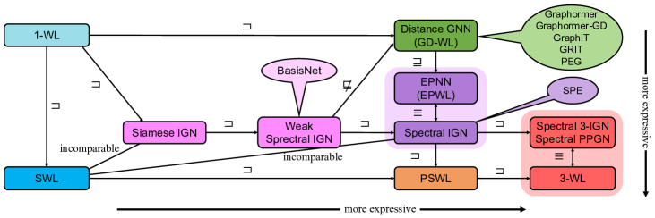
Finally, we discuss the potential of using spectral features to boost the expressive power of higher-order GNNs. We show using the projection matrices alone does not provide any additional expressive power advantage when combined with highly expressive GNNs such as PPGN and -IGN (Maron et al., 2019b, a). Nevertheless, we propose a possible solution towards further expressiveness gains: we hypothesize that stronger expressivity could be achieved through higher-order extensions of graph spectra, such as projection tensors. Overall, our theoretical results characterize an expressiveness hierarchy across basis invariant GNNs, distance-based GNNs, GTs with spectral encoding, subgraph-based GNNs, and higher-order GNNs. The resulting hierarchy is illustrated in Figure 1.
2 Related GNN Models
2.1 Spectrally-enhanced GNNs
In recent years, a multitude of research has emerged to develop spectrally-enhanced GNNs/GTs, integrating graph spectral information into either GNN node features or the subsequent message-passing process. These endeavors can be categorized into the following three groups.
Laplacian eigenvectors as absolute positional encoding. One way to design spectrally-enhanced GNNs involves encoding Laplacian eigenvectors. This approach treats each eigenvector as a 1-dimensional node feature and incorporates the top eigenvectors as a type of absolute positional encoding, which can be used to enhance any message-passing GNNs and GTs (Dwivedi et al., 2020; Dwivedi & Bresson, 2021; Kreuzer et al., 2021; Rampasek et al., 2022; Maskey et al., 2022; Dwivedi et al., 2022; Kim et al., 2022). However, one main drawback of using Laplacian eigenvectors arises from the ambiguity problem. Such ambiguity creates severe issues regarding training instability and poor generalization (Wang et al., 2022). While this problem can be partially mitigated through techniques like randomly flipping eigenvector signs or employing a canonization method (Ma et al., 2023a), it becomes much more complicated when eigenvalues have higher multiplicities.
Spectral invariant architectures. A better approach would be to design GNNs that are invariant w.r.t. the choice of eigenvectors. For example, SignNet (Lim et al., 2023) transforms each eigenvector to for some permutation equivariant function , which guarantees the invariance when all eigenvalues have a multiplicity of 1. In case of higher multiplicity, BasisNet (Lim et al., 2023) achieves spectral invariance for the first time by utilizing the projection matrix. Specifically, given an eigenvalue with multiplicity , the projection matrix defined as is invariant w.r.t. the choice of (unit) eigenvectors as long as they form an orthogonal basis of the eigenspace associated with . Therefore, BasisNet simply feeds the projection matrix into a permutation equivariant model (e.g., 2-IGN (Maron et al., 2019b)) to generate spectral invariant node features . The node features generated for different eigenspaces are concatenated together. While the authors proved that BasisNet can universally represent any graph functions when is universal (e.g., using -IGN), the empirical performance is generally unsatisfactory when employing a practical model (i.e., 2-IGN). Recently, Huang et al. (2024) further generalized BasisNet by proposing SPE, which performs a soft aggregation across different eigenspaces rather than a hard separation implemented in BasisNet. Specifically, let be an orthogonal basis of (unit) eigenvectors associated with eigenvalues , respectively; then, each 1-dimensional node feature generated by SPE has the form , where is a parameterized function associated with feature dimension . The authors demonstrated that SPE can enhance the stability and generalization of GNNs, yielding much better empirical performance compared with BasisNet.
Spectral distances as invariant relative positional encoding. In contrast to encoding Laplacian eigenvectors, an alternative approach to achieving spectral invariance involves utilizing (spectral) distances. Previous studies have identified various distances, spanning from the basic shortest path distance (Feng et al., 2022; Abboud et al., 2022) to more advanced ones such as PageRank distance, resistance distance, and distances associated with random walks and graph diffusion (Li et al., 2020; Zhang et al., 2023b; Mialon et al., 2021; Feldman et al., 2023). Notably, all of these distances have a deep relation to the graph Laplacian while being more interpretable than eigenvectors and not suffering from ambiguity problems. The work of PEG (Wang et al., 2022) designed an invariant relative positional encoding based on Laplacian eigenvectors, which can also be treated as a distance between nodes. Distances can be easily encoded in GNN models by either serving as edge features in message-passing aggregations (Wang et al., 2022; Velingker et al., 2023) or as relative positional encoding in Graph Transformers (Ying et al., 2021; Zhang et al., 2023a; Ma et al., 2023b).
2.2 Expressive GNNs
The expressive power of GNNs has been studied in depth in the recent few years. Early works (Xu et al., 2019; Morris et al., 2019) have pointed out a fundamental limitation of GNNs by establishing an equivalence between message-passing neural networks and the 1-WL graph isomorphism test (Weisfeiler & Lehman, 1968). To develop more expressive models, several studies leveraged high-dimensional variants of the WL test (Cai et al., 1992; Grohe, 2017). Representative models include -IGN (Maron et al., 2019b), PPGN (Maron et al., 2019a), and -GNN (Morris et al., 2019, 2020). However, these models suffer from severe computational costs and are generally not suitable in practice. Currently, one mainstream approach to designing simple, efficient, practical, and expressive architectures is the Subgraph GNNs (Cotta et al., 2021; Bevilacqua et al., 2022, 2023; You et al., 2021; Zhang & Li, 2021; Zhao et al., 2022; Kong et al., 2023). In particular, the expressive power of Subgraph GNNs as well as their relation to the WL tests are well-understood in recent studies (Frasca et al., 2022; Qian et al., 2022; Zhang et al., 2023a, 2024). These results will be used to analyze spectrally-enhanced GNNs in this paper.
2.3 Expressive power of spectral invariant GNNs
While spectrally-enhanced GNNs have been extensively studied in the literature, much less is known about their expressive power. Balcilar et al. (2021); Wang & Zhang (2022) delved into the expressive power of specific spectral filtering GNNs, but their expressive power is inherently limited by 1-WL. Another line of works studied the expressive power of the raw spectral invariants (e.g., projection matrices) in relation to the Weisfeiler-Lehman algorithms (Fürer, 1995, 2010; Rattan & Seppelt, 2023). However, their analysis does not consider any aggregation or refinement procedures over spectral invariants, and thus, it does not provide explicit insights into the expressive power of the corresponding GNNs. Lim et al. (2023) proposed a concrete spectral invariant GNN called BasisNet, but their expressiveness analysis still largely focuses on raw eigenvectors and projection matrices. To our knowledge, none of the prior works addresses the crucial problem of whether/how the design of GNN layers contributes to the model’s expressiveness. In this paper, we will answer this question by showing that a suitable aggregation procedure can strictly improve the expressive power beyond raw spectral features, and different aggregation schemes can lead to considerable variations in the models’ expressiveness.
3 Preliminaries
We use and to denote sets and multisets, respectively. Given a (multi)set , its cardinality is denoted as . In this paper, we consider finite, undirected, simple graphs with no isolated vertices. Let be a graph with vertex set and edge set , where each edge in is represented as a set of cardinality two. The neighbors of a vertex is denoted as , and the degree of is denoted as . Given vertex pair , denote by its atomic type, which encodes whether , , or and are not adjacent. Given vertex tuple , the rooted graph is a graph obtained from by marking vertices sequentially. We denote by the set of all graphs and by the set of all rooted graphs marking vertices. It follows that .
Graph invariant. Two (rooted) graphs are called isomorphic (denoted by ) if there is a bijection such that for all , and for all vertices , iff . A function defined on graphs is called a graph invariant if it is invariant under isomorphism, i.e., if . In the context of graph learning, any GNN that outputs a graph representation should be a graph invariant over ; similarly, any GNN that outputs a representation for each node/each pair of nodes should be a graph invariant over /, respectively.
Graph vectors and matrices. Any real-valued graph invariant defined over corresponds to a graph vector when restricting on a specific graph . Without ambiguity, we denote the elements in as for each , which is equal to . Similarly, any real-valued graph invariant defined over corresponds to a graph matrix when restricting on , where element equals to . For ease of reading, we will drop the subscript when there is no ambiguity of the graph used in context. One can generalize all basic linear algebras from classic vectors/matrices to those defined on graphs. For example, the matrix product is defined as . Several basic graph matrices include the adjacency matrix , degree matrix , Laplacian matrix , and normalized Laplacian matrix . Note that all these matrices are symmetric.
Graph spectra and projection. Let be any symmetric graph matrix (e.g., , , or ). The graph spectrum is the set of all eigenvalues of , which is a graph invariant over . In addition to eigenvalues, the spectral information of a graph also includes eigenvectors or eigenspaces, which contain much more fine-grained information. Unfortunately, eigenvectors have inherent ambiguity and cannot serve as a valid graph invariant over . Instead, we focus on the eigenspaces characterized by their projection matrices. Concretely, there is a unique projection matrix for each eigenvalue , which can be obtained via the eigen-decomposition , where is the number of different eigenvalues. It follows that these projection matrices are symmetric, idempotent (), “orthogonal” ( for all ), and sum to identity (). There is a close relation between projection matrix and any orthogonal basis of unit eigenvectors that spans the eigenspace associated with : specifically, . The projection matrices naturally define a graph invariant over :
We call the eigenspace projection invariant (associated with graph matrix ).
4 Eigenspace Projection Network
This section introduces a simple GNN design paradigm based on the invariant defined above, called Eigenspace Projection GNN (EPNN). The idea of EPNN is very simple: essentially encodes the relation between vertices and in graph and can thus be treated as a form of “edge feature”. In light of this, one can naturally define a message-passing GNN that updates the node representation of each vertex by iteratively aggregating the representations of other nodes along with edge features associated with . Formally, consider a -layer EPNN and denote by the node representation of computed by an EPNN after the -th layer. Then, we can write the update rule of each EPNN layer as follows:
| (1) | ||||
where all node representations are the same at initialization. Here, can be any parameterized function representing the -th layer. In practice, it can be implemented in various ways such as GIN-based aggregation (Xu et al., 2019) or Graph Transformers (Ying et al., 2021), and we highlight that it is particularly suited for Graph Transformers as the graph becomes fully connected with this edge feature. Finally, after the -th layer, a global pooling is performed over all vertices in the graph to obtain the graph representation .
EPNN is well-defined. First, the graph representation computed by an EPNN is permutation invariant w.r.t. vertices, as is a graph invariant over . Second, EPNN does not suffer from the eigenvector ambiguity problem, as is uniquely determined by graph . Later, we will show that EPNN can serve as a simple yet unified framework for studying the expressive power of spectral invariant GNNs.
4.1 Expressive power of EPNN
The central question we would like to study is: what is the expressive power of EPNN? To formally study this question, this subsection introduces EPWL (Eigenspace Projection Weisfeiler-Lehman), an abstract color refinement algorithm tailored specifically for graph isomorphism test. Compared with Equation 1, in EPWL the node representation is replaced by a color , and the aggregation function is replaced by a perfect hash function , as presented below:
| (2) |
Initially, all node colors are the same. For each iteration , the color mapping induces an equivalence relation over vertex set , and the relation gets refined with the increase of . Therefore, with a sufficiently large number of iterations , the relations get stable. The graph representation is then defined to be the multiset of stable colors. EPWL distinguishes two non-isomorphic graphs iff the computed graph representations are different. We have the following result (which can be easily proved following standard techniques, see e.g., Zhang et al. (2023a)):
Proposition 4.1.
The expressive power of EPNN is bounded by EPWL in terms of graph isomorphism test. Moreover, with sufficient layers and proper functions , EPNN can be as expressive as EPWL.
In subsequent analysis, we will bound the expressive power of EPWL by building relations to the standard Weisfeiler-Lehman hierarchy. First, it is easy to see that EPWL is lower bounded by the classic 1-WL defined below:
| (3) |
where is the 1-WL color of in graph after iterations. This result follows from the fact that the EPWL color mapping always induces a finer relation than the 1-WL color mapping , as is fully encoded in (see Lemma A.5). Besides, it is easy to give 1-WL indistinguishable graphs that can be distinguished via spectral information (see Figure 2). Putting these together, we arrive at the following conclusion:
Proposition 4.2.
For any graph matrix , the corresponding EPWL is strictly more expressive than 1-WL in distinguishing non-isomorphic graphs.
On the other hand, the question becomes more intriguing when studying the upper bound of EPWL. Below, we will approach the problem by building fundamental connections between EPWL and an important class of expressive GNNs known as Subgraph GNNs. The basic form of Subgraph GNN is very simple: given a graph , it treats as a set of rooted graphs (known as node marking), independently runs 1-WL for each , and finally merges their graph representations. We call the above algorithm SWL, and the refinement rule can be formally written as
| (4) | ||||
where is the SWL color of vertex in graph after iterations, and the initial color distinguishes the marked vertex in . Recently, Zhang et al. (2023a); Frasca et al. (2022) significantly generalized Subgraph GNNs by enabling interactions among different subgraphs and built a complete design space. Among them, Zhang et al. (2023a) proposed the PSWL algorithm, which adds a cross-graph aggregation to SWL as shown below:
| (5) | ||||
where is the PSWL color of after iterations. We now present our main result, which reveals a fundamental connection between PSWL and EPWL:
Theorem 4.3.
For any graph matrix , the expressive power of EPWL is strictly bounded by PSWL in distinguishing non-isomorphic graphs.
The proof of Theorem 4.3 is deferred to Section A.3, which is based on the recent graph theory result established by Rattan & Seppelt (2023). Specifically, given any graph and vertices , each projection element in is determined by the SWL stable color for any symmetric “equitable” matrix defined in Rattan & Seppelt (2023), and the eigenvalues are also determined by the SWL graph representation. Notably, all matrices studied in this paper (e.g., ) are equitable. Based on this result, one may guess that EPWL can be bounded by SWL. However, we show this is actually not the case when further taking the message-passing aggregation into account. The key technical contribution in our proof is to relate the refinement procedure in EPWL to the additional cross-graph aggregation in PSWL. To this end, we show the stable color is strictly finer than the stable color , thus concluding the proof.
Remark 4.4.
Based on Theorem 4.3, one can also bound the expressiveness of EPWL by other popular GNNs in literature, such as SSWL (Zhang et al., 2023a), Local 2-GNN (Morris et al., 2020; Zhang et al., 2024), (Frasca et al., 2022), ESAN (Bevilacqua et al., 2022), and GNN-AK (Zhao et al., 2022), as all these architectures are more expressive than PSWL (Zhang et al., 2023a). However, EPWL is incomparable to the vanilla SWL, where we give counterexamples in Section A.8.
The significance of Theorem 4.3 is twofold. First, it reveals a surprising relation between GNNs augmented with spectral information and the ones grounded in structural message-passing, which represents two seemingly unrelated research directions. Our result thus offers insights into how previously proposed expressive GNNs can encode spectral information. Second, Theorem 4.3 points out a fundamental limitation of EPNN. Indeed, combined with the result that PSWL is strictly bounded by 3-WL (Zhang et al., 2023a, 2024), we obtain the concluding corollary:
Corollary 4.5.
For any graph matrix , the expressive power of EPWL is strictly bounded by 3-WL.
5 Distance GNNs and Graph Transformers
In this section, we will show that EPNN unifies all distance-based spectral invariant GNNs. Here, we adopt the framework proposed in Zhang et al. (2023b), known as Generalized Distance (GD) GNNs. The aggregation formula of the corresponding GD-WL can be written as follows:
| (6) | ||||
where is the GD-WL color of vertex after iterations, and can be any valid distance metric. By choosing different distances, GD-WL incorporates various prior works listed below.
- •
-
•
Resistance distance (RD). It is defined to be the effective resistance between two nodes when treating the graph as an electrical network where each edge has a resistance of . Recently, Zhang et al. (2023b) showed that incorporating RD can significantly improve the expressive power of GNNs for biconnectivity problems such as identifying cut vertices/edges. Besides, RD has been extensively studied in other areas in the GNN community, such as alleviating oversquashing problems (Arnaiz-Rodríguez et al., 2022).
-
•
Distances based on random walk. The hitting-time distance (HTD) between two vertices and is defined as the expected number of steps in a random walk starting from and reaching for the first time, which is an asymmetric distance. Instead, the commute-time distance (CTD) is defined as the expected number of steps for a round-trip starting at to reach and then return to , which is a symmetrized version of HTD. These distances are fundamental in graph theory and have been used to develop/understand expressive GNNs (Velingker et al., 2023; Zhang et al., 2023a).
-
•
PageRank distance (PRD). Given weight sequence , the PageRank distance between vertices and is defined as , where is the random walk probability matrix. It is a generalization of the -step landing probability distance, which corresponds to setting and for all . Li et al. (2020) first proposed to use PRD-WL to boost the expressive power of GNNs.
-
•
Other distances. We also study the (normalized) diffusion distance (Coifman & Lafon, 2006) and the biharmonic distance (Lipman et al., 2010). Due to space limit, please refer to Section A.4 for more details.
Our main result is stated as follows:
Theorem 5.1.
For any distance listed above, the expressive power of GD-WL is upper bounded by EPWL with the normalized graph Laplacian matrix .
The proof of Theorem 4.3 is highly technical and is deferred to Section A.4, with several important remarks made as follows. For the case of SPD, the proof is based on the key finding that determines the shortest path distance between and for any graph and vertices . Unfortunately, this property does not transfer to other distances listed above. For general distances, the reason why EPWL is still more expressive lies in the entire message-passing process (or color refinement procedure). Concretely, the refinement continuously enriches the information embedded in node colors , so that the tuple eventually encompasses sufficient information to determine any distance (although alone may not determine it). Our proof thus emphasizes the critical role of message-passing aggregation in enhancing the expressiveness of spectral information. Note that this is also justified in the proof of Theorem 4.3, where the message-passing process boosts the expressive power of EPWL beyond SWL. Moreover, we emphasize that these distances listed above cannot be well-encoded when using weaker message-passing aggregations, as will be elucidated in Section 6.2.
Implications. Theorem 5.1 has a series of consequences. First, it implies that all the power of distance information is possessed by EPWL. As an example, we immediately have the following corollary based on the relation between distance and biconnectivity of a graph established in Zhang et al. (2023b), which significantly extends the classic result that Laplacian spectrum encodes graph connectivity (Brouwer & Haemers, 2011).
Corollary 5.2.
EPWL is fully expressive for encoding graph biconnectivity properties, such as identifying cut vertices and cut edges, determining the number of biconnected components, and distinguishing graphs with non-isomorphic block cut-vertex trees and block cut-edge trees.
Remark 5.3.
Corollary 5.2 offers a novel understanding of the work by Zhang et al. (2023b) on why ESAN can encode graph biconnectivity, thereby thoroughly unifying their analysis. Essentially, this is just because ESAN is more powerful than EPWL (Remark 4.4), and EPWL itself is already capable of encoding both SPD and RD.
Remark 5.4.
Combining Theorems 4.3 and 5.1 resolves an open question posed by Zhang et al. (2023a), confirming that PSWL can encode resistance distance.
As a second implication, combined with Corollary 4.5, Theorem 5.1 highlights a fundamental limitation of all distance-based GNNs as stated below:
Corollary 5.5.
For any distance defined above, the expressive power of GD-WL is strictly bounded by 3-WL.
Distances as positional encoding. Distances have also found extensive application as positional encoding in GNNs and GTs. For instance, Graphormer (Ying et al., 2021), Graphormer-GD (Zhang et al., 2023b), and GraphiT (Mialon et al., 2021) employ various distances as relative positional encoding in Transformer’s attention layers. Similarly, GRIT (Ma et al., 2023b) employs multi-dimensional PRD and a novel attention mechanism to further boost the performance of GTs. The positional encoding devised in PEG (Wang et al., 2022) can also be viewed as a function of a distance, with the architecture representing an instantiation of GD-WL. These architectures are analyzed in Section A.7, where we have the following concluding corollary:
Corollary 5.6.
The expressive power of Graphormer, Graphormer-GD, GraphiT, GRIT, and PEG are all bounded by EPWL and strictly less expressive than 3-WL.
6 Spectral Invariant Graph Network
To gain an in-depth understanding of the expressive power of EPNN, in this section we will switch our attention to a more principled perspective by studying how to model spectral invariant GNNs based on the symmetry of projection matrices. Consider a graph with vertex set . We can group all spectral information of into a 4-dimensional tensor , where encodes the -th eigenvalue and encodes the -th element of the projection matrix associated with . From this representation, one can easily figure out the symmetry group associated with , which is the product group of two permutation groups and representing two independent symmetries — eigenspace symmetry and graph symmetry. For any element , it acts on in the following way:
| (7) |
We would like to design a GNN model that is invariant under , i.e., for all . Interestingly, this setting precisely corresponds to a specific case of the DSS framework proposed in Maron et al. (2020); Bevilacqua et al. (2022). This offers a theoretically inspired approach to designing powerful invariant architectures, as we will detail below.
6.1 Spectral IGN
In the DSS framework, the neural network is formed by stacking a series of equivariant linear layers interleaved with elementwise non-linear activation , culminating in the final pooling layer:
| (8) |
where each is equivariant w.r.t. , i.e., for all ,
is an invariant pooling layer (e.g., average pooling or max pooling), and is a multi-layer perceptron. Here, the key question lies in designing linear layers equivariant to the product group . Maron et al. (2020) theoretically showed that can be decomposed in the following way:
| (9) |
where are two linear functions equivariant to the graph symmetry modeled by . This decomposition is significant as the design space of equivariant linear layers for graphs has been fully characterized in Maron et al. (2019b), known as 2-IGN. We thus call our model (Equations 8 and 9) Spectral IGN.
The central question we would like to study is: what is the expressive power of Spectral IGN? Surprisingly, we have the following main result:
Theorem 6.1.
The expressive power of Spectral IGN is bounded by EPWL. Moreover, with sufficient layers and proper network parameters, Spectral IGN is as expressive as EPWL in distinguishing non-isomorphic graphs.
The proof of Theorem 6.1 is given in Section A.5. It offers an interesting and alternative view for theoretically understanding the EPNN designing framework and justifying its expressiveness. Moreover, the connection to Spectral IGN allows us to bridge EPNN with important architectural variants as we will discuss in the next subsection.
Remark 6.2.
We remark that there is a variant of Spectral IGN, where the pooling layer is decomposed into two pooling layers via with and pooling layers for symmetry groups and , respectively. This variant has the same expressive power, and Theorem 6.1 still holds.
6.2 Siamese IGN
Let us consider an interesting variant of Spectral IGN, dubbed Siamese IGN (Maron et al., 2020), where the network processes each eigenspace () independently using a “Siamese” 2-IGN without aggregating over different eigenspaces. This corresponds to replacing Equation 9 by with a 2-IGN layer. Siamese IGN is interesting because it is a special type of Spectral IGN that is invariant to a strictly larger group formed by the wreath product (see Maron et al., 2020; Wang et al., 2020). Moreover, it is closely related to a prior architecture called BasisNet (Lim et al., 2023, see Section A.6 for a detailed description), as BasisNet also processes each eigenspace independently without interaction. To elaborate on this connection, consider a variant of Siamese IGN, dubbed Weak Spectral IGN, which is obtained from Siamese IGN by decomposing the pooling layer according to Remark 6.2. Note that unlike Siamese IGN, Weak Spectral IGN is no longer invariant to group . We have the following result:
Proposition 6.3.
Let the top graph encoder used in BasisNet be any 1-layer message-passing GNN. Then, the expressive power of BasisNet is bounded by Weak Spectral IGN.
On the other hand, a more fundamental question lies in the relation between Siamese IGN, Weak Spectral IGN, and Spectral IGN. Our main result states that there are strict expressivity gaps between them:
Theorem 6.4.
Siamese IGN is strictly less expressive than Weak Spectral IGN. Moreover, Weak Spectral IGN is strictly less expressive than Spectral IGN.
Discussions with BasisNet. Combined with previous results, one can prove that EPNN is strictly more expressive than BasisNet222This holds for any message-passing-based top graph encoder with arbitrary layers by following the construction in Theorem 6.4.. This result is particularly striking, as EPNN only stores node representations while BasisNet stores a representation for each 3-tuple , whose memory complexity scales like . Combined with Corollary 4.5, we conclude that the expressive power of BasisNet is also strictly bounded by 3-WL.
Discussions with SPE. We next turn to the SPE architecture (Huang et al., 2024). Surprisingly, while SPE was originally designed to improve the stability and generalization of spectral invariant GNNs (see Section 2.1), we found the soft aggregation across different eigenspaces simultaneously enhances the network’s expressive power. Indeed, we have:
Proposition 6.5.
When 2-IGN is used to generate node features in SPE and the top graph encoder is a message-passing GNN, the expressive power of the whole SPE architecture is as expressive as Spectral IGN.
Proposition 6.5 theoretically justifies the design of SPE. Combined with previous results, we conclude that SPE is strictly more expressive than BasisNet when using the same 2-IGN backbone, while being strictly bounded by 3-WL.
Delving more into the gap. We remark that the gap between Siamese IGN and Spectral IGN is not just theoretical; it also reveals significant limitations of the siamese design in practical aspects. Specifically, we identify that both Siamese IGN and Weak Spectral IGN cannot fully encode any graph distance listed in Section 5 (even the basic SPD), as stated in the following theorem:
Theorem 6.6.
For any distance listed in Section 5, there exist two non-isomorphic graphs which GD-WL can distinguish but Weak Spectral IGN (applied to matrix ) cannot.
On the other hand, we have proved that EPNN applied to matrix is more powerful than GD-WL. This contrast reveals the crucial role of allowing interaction between eigenspaces for enhancing model’s expressiveness.
6.3 Extending to higher-order spectral invariant GNNs
The DSS framework presented in Section 6.1 is quite general. In principle, any -equivariant graph layer can be used to build a GNN model invariant to . This can be achieved by making in Equation 9 two instantiations of . In this subsection, we will study higher-order spectral invariant GNNs where the used graph encoders are beyond 2-IGN. We consider two standard settings for choosing highly expressive graph encoders: the -IGN and the -order Folklore GNN (Maron et al., 2019b, a; Azizian et al., 2021). We call the resulting models Spectral -IGN and Spectral -FGNN, respectively. Unfortunately, our results are negative for all of these higher-order spectral invariant GNNs:
Proposition 6.7.
For all , Spectral -IGN is as expressive as -WL. Similarly, for all , Spectral -FGNN is as expressive as -FWL.
We give a proof in Section A.7. Combined with the results that -IGN is already as expressive as -WL and -FGNN is already as expressive as -FWL (Maron et al., 2019a; Azizian et al., 2021; Geerts & Reutter, 2022), we conclude that commonly-used spectral information does not help when combined with highly powerful GNN designs.
Discussions on higher-order spectral features. The above negative result further inspires us to think about the following question: is it still possible to use spectral information to enhance the expressive power of higher-order GNNs? Here, we offer some possible directions towards this goal. The crux here is to use higher-order spectral features. Specifically, all the spectral information considered in previous sections (e.g., distance or projection matrices) is at most 2-dimensional. Can we generalize these spectral features into multi-dimensional tensors? This is indeed possible: for example, a simple approach is to use symmetric powers of a graph (also called the token graph), which has been widely studied in literature (Audenaert et al., 2007; Alzaga et al., 2010; Barghi & Ponomarenko, 2009; Fabila-Monroy et al., 2012). The -th symmetric power of graph , denoted by , is the graph formed by vertex set and edge set . Here, each element in is a multiset of cardinality , and two multisets are connected if their symmetric difference is an edge. In this way, one can easily define higher-order spectral information based on (the eigenspace projection invariant associated with the -th token graph), e.g., by setting . The higher-order spectral information can then serve as initial features of any higher-order GNN that computes representations for each vertex tuple, such as -IGN.
Several works have pointed out the strong expressive power of higher-order spectral features. Audenaert et al. (2007) verified that the spectra of the 3rd symmetric power are already not less expressive than 3-WL. Moreover, Alzaga et al. (2010); Barghi & Ponomarenko (2009) upper bounds the expressive power of the spectra of the -th symmetric power by -FWL. These results imply that using higher-order projection tensors is a promising approach to further boosting the expressive power of higher-order GNNs. We leave the corresponding architectural design and expressiveness analysis as an open direction for future study.
7 Experiments
In this section, we empirically evaluate the expressive power of various GNN architectures studied in this paper. We adopt the BREC benchmark (Wang & Zhang, 2023), a comprehensive dataset for comparing the expressive power of GNNs. We focus on the following GNNs that are closely related to this paper: Graphormer (Ying et al., 2021) (a distance-based GNN that uses SPD, see Section 5); NGNN (Zhang & Li, 2021) (a variant of subgraph GNN, see Section 4.1); ESAN (Bevilacqua et al., 2022) (an advanced subgraph GNN that adds cross-graph aggregations, see Section 4.1); PPGN (Maron et al., 2019a) (a higher-order GNN, see Section 6.3); EPNN (this paper). We follow the same setup as in Wang & Zhang (2023) in both training and evaluation. For all baseline GNNs, the reported numbers are directly borrowed from Wang & Zhang (2023); For EPNN, we run the model 10 times with different seeds and report the average performance333Our code can be found in the following github repo:
https://github.com/LingxiaoShawn/EPNN-Experiments.
| Model | WL class | Basic | Reg | Ext | CFI | Total |
|---|---|---|---|---|---|---|
| Graphormer | SPD-WL | 26.7 | 10.0 | 41.0 | 10.0 | 19.8 |
| NGNN | SWL | 98.3 | 34.3 | 59.0 | 0 | 41.5 |
| ESAN | GSWL | 96.7 | 34.3 | 100.0 | 15.0 | 55.2 |
| PPGN | 3-WL | 100.0 | 35.7 | 100.0 | 23.0 | 58.2 |
| EPNN | EPWL | 100.0 | 35.7 | 100.0 | 5.0 | 53.8 |
The results are presented in Table 1. From these results, one can see that the empirical performance of EPNN matches its theoretical expressivity in our established hierarchy. Concretely, EPNN performs much better than Graphormer (SPD-WL) and NGNN (SWL), while underperforming ESAN (GS-WL) and PPGN (3-WL).
8 Conclusion
This paper investigates the expressive power of spectral invariant GNNs and related models. It establishes an expressiveness hierarchy between current models using a unifying framework we propose. We also draw a surprising connection to a recently proposed class of highly expressive GNNs, demonstrating that specific instances from this class (e.g., PSWL) upper bound all spectral invariant GNNs. This implies spectral invariant GNNs are strictly less expressive than the 3-WL test. Furthermore, we show spectral projection features and spectral distances do not provide additional expressivity benefits when combined with more powerful high-order architectures. We give a graphical illustration of all of these results in Figure 1.
Open questions. There are still several promising directions that are not fully explored in this paper. First, an interesting question lies in how the choice of graph matrix affects the expressive power of spectral invariant GNNs. We suspect that using (normalized) Laplacian matrix can be more beneficial than using the adjacency matrix, and the former is strictly more expressive. We have given implicit evidence showing that EPNN with matrix can encode all distances studied in this paper; however, we were unable to demonstrate the same result for other graph matrices. Besides, another important open question is the expressive power of higher-order spectral features, such as the one obtained by using token graphs. It is still unknown about a tight lower/upper bound of their expressive power in relation to higher-order WL tests. Moreover, investigating the refinements over higher-order spectral features and the corresponding GNNs could be a fantastic open direction.
Impact Statement
This paper presents work whose goal is to advance the field of Machine Learning. There are many potential societal consequences of our work, none of which we feel must be specifically highlighted here.
Acknowledgements
HM is the Robert J. Shillman Fellow and is supported by the Israel Science Foundation through a personal grant (ISF 264/23) and an equipment grant (ISF 532/23). BZ would like to thank Jingchu Gai for helpful discussions.
References
- Abboud et al. (2022) Abboud, R., Dimitrov, R., and Ceylan, I. I. Shortest path networks for graph property prediction. In The First Learning on Graphs Conference, 2022.
- Alzaga et al. (2010) Alzaga, A., Iglesias, R., and Pignol, R. Spectra of symmetric powers of graphs and the weisfeiler–lehman refinements. Journal of Combinatorial Theory, Series B, 100(6):671–682, 2010.
- Arnaiz-Rodríguez et al. (2022) Arnaiz-Rodríguez, A., Begga, A., Escolano, F., and Oliver, N. M. Diffwire: Inductive graph rewiring via the lovász bound. In The First Learning on Graphs Conference, 2022.
- Audenaert et al. (2007) Audenaert, K., Godsil, C., Royle, G., and Rudolph, T. Symmetric squares of graphs. Journal of Combinatorial Theory, Series B, 97(1):74–90, 2007. ISSN 0095-8956.
- Azizian et al. (2021) Azizian, W. et al. Expressive power of invariant and equivariant graph neural networks. In International Conference on Learning Representations, 2021.
- Balcilar et al. (2021) Balcilar, M., Renton, G., Héroux, P., Gaüzère, B., Adam, S., and Honeine, P. Analyzing the expressive power of graph neural networks in a spectral perspective. In International Conference on Learning Representations, 2021.
- Barghi & Ponomarenko (2009) Barghi, A. R. and Ponomarenko, I. Non-isomorphic graphs with cospectral symmetric powers. the electronic journal of combinatorics, pp. R120–R120, 2009.
- Bevilacqua et al. (2022) Bevilacqua, B., Frasca, F., Lim, D., Srinivasan, B., Cai, C., Balamurugan, G., Bronstein, M. M., and Maron, H. Equivariant subgraph aggregation networks. In International Conference on Learning Representations, 2022.
- Bevilacqua et al. (2023) Bevilacqua, B., Eliasof, M., Meirom, E., Ribeiro, B., and Maron, H. Efficient subgraph gnns by learning effective selection policies. arXiv preprint arXiv:2310.20082, 2023.
- Brouwer & Haemers (2011) Brouwer, A. E. and Haemers, W. H. Spectra of graphs. Springer Science & Business Media, 2011.
- Cai et al. (1992) Cai, J.-Y., Fürer, M., and Immerman, N. An optimal lower bound on the number of variables for graph identification. Combinatorica, 12(4):389–410, 1992.
- Coifman & Lafon (2006) Coifman, R. R. and Lafon, S. Diffusion maps. Applied and computational harmonic analysis, 21(1):5–30, 2006.
- Cotta et al. (2021) Cotta, L., Morris, C., and Ribeiro, B. Reconstruction for powerful graph representations. Advances in Neural Information Processing Systems, 34:1713–1726, 2021.
- Dwivedi & Bresson (2021) Dwivedi, V. P. and Bresson, X. A generalization of transformer networks to graphs. AAAI Workshop on Deep Learning on Graphs: Methods and Applications, 2021.
- Dwivedi et al. (2020) Dwivedi, V. P., Joshi, C. K., Luu, A. T., Laurent, T., Bengio, Y., and Bresson, X. Benchmarking graph neural networks. arXiv preprint arXiv:2003.00982, 2020.
- Dwivedi et al. (2022) Dwivedi, V. P., Luu, A. T., Laurent, T., Bengio, Y., and Bresson, X. Graph neural networks with learnable structural and positional representations. In International Conference on Learning Representations, 2022.
- Fabila-Monroy et al. (2012) Fabila-Monroy, R., Flores-Peñaloza, D., Huemer, C., Hurtado, F., Urrutia, J., and Wood, D. R. Token graphs. Graphs and Combinatorics, 2012.
- Feldman et al. (2023) Feldman, O., Boyarski, A., Feldman, S., Kogan, D., Mendelson, A., and Baskin, C. Weisfeiler and leman go infinite: Spectral and combinatorial pre-colorings. Transactions on Machine Learning Research, 2023. ISSN 2835-8856.
- Feng et al. (2022) Feng, J., Chen, Y., Li, F., Sarkar, A., and Zhang, M. How powerful are k-hop message passing graph neural networks. In Advances in Neural Information Processing Systems, volume 35, pp. 4776–4790, 2022.
- Frasca et al. (2022) Frasca, F., Bevilacqua, B., Bronstein, M. M., and Maron, H. Understanding and extending subgraph gnns by rethinking their symmetries. In Advances in Neural Information Processing Systems, 2022.
- Fürer (1995) Fürer, M. Graph isomorphism testing without numerics for graphs of bounded eigenvalue multiplicity. In Proceedings of the sixth annual ACM-SIAM symposium on Discrete algorithms, pp. 624–631, 1995.
- Fürer (2001) Fürer, M. Weisfeiler-lehman refinement requires at least a linear number of iterations. In International Colloquium on Automata, Languages, and Programming, pp. 322–333. Springer, 2001.
- Fürer (2010) Fürer, M. On the power of combinatorial and spectral invariants. Linear algebra and its applications, 432(9):2373–2380, 2010.
- Geerts & Reutter (2022) Geerts, F. and Reutter, J. L. Expressiveness and approximation properties of graph neural networks. In International Conference on Learning Representations, 2022.
- Grohe (2017) Grohe, M. Descriptive complexity, canonisation, and definable graph structure theory, volume 47. Cambridge University Press, 2017.
- Huang et al. (2024) Huang, Y., Lu, W., Robinson, J., Yang, Y., Zhang, M., Jegelka, S., and Li, P. On the stability of expressive positional encodings for graph neural networks. In International Conference on Learning Representations, 2024.
- Kim et al. (2022) Kim, J., Nguyen, D., Min, S., Cho, S., Lee, M., Lee, H., and Hong, S. Pure transformers are powerful graph learners. In Advances in Neural Information Processing Systems, volume 35, pp. 14582–14595, 2022.
- Klein & Randic (1993) Klein, D. J. and Randic, M. Resistance distance. Journal of Mathematical Chemistry, 12:81–95, 1993.
- Kong et al. (2023) Kong, L., Feng, J., Liu, H., Tao, D., Chen, Y., and Zhang, M. Mag-gnn: Reinforcement learning boosted graph neural network. arXiv preprint arXiv:2310.19142, 2023.
- Kreuzer et al. (2021) Kreuzer, D., Beaini, D., Hamilton, W., Létourneau, V., and Tossou, P. Rethinking graph transformers with spectral attention. Advances in Neural Information Processing Systems, 34:21618–21629, 2021.
- Li et al. (2020) Li, P., Wang, Y., Wang, H., and Leskovec, J. Distance encoding: design provably more powerful neural networks for graph representation learning. In Proceedings of the 34th International Conference on Neural Information Processing Systems, pp. 4465–4478, 2020.
- Lim et al. (2023) Lim, D., Robinson, J. D., Zhao, L., Smidt, T., Sra, S., Maron, H., and Jegelka, S. Sign and basis invariant networks for spectral graph representation learning. In The Eleventh International Conference on Learning Representations, 2023.
- Lipman et al. (2010) Lipman, Y., Rustamov, R. M., and Funkhouser, T. A. Biharmonic distance. ACM Transactions on Graphics (TOG), 29(3):1–11, 2010.
- Ma et al. (2023a) Ma, G., Wang, Y., and Wang, Y. Laplacian canonization: A minimalist approach to sign and basis invariant spectral embedding. In Thirty-seventh Conference on Neural Information Processing Systems, 2023a.
- Ma et al. (2023b) Ma, L., Lin, C., Lim, D., Romero-Soriano, A., Dokania, P. K., Coates, M., Torr, P., and Lim, S.-N. Graph inductive biases in transformers without message passing. In Proceedings of the 40th International Conference on Machine Learning, volume 202, pp. 23321–23337. PMLR, 2023b.
- Maron et al. (2019a) Maron, H., Ben-Hamu, H., Serviansky, H., and Lipman, Y. Provably powerful graph networks. In Advances in neural information processing systems, volume 32, 2019a.
- Maron et al. (2019b) Maron, H., Ben-Hamu, H., Shamir, N., and Lipman, Y. Invariant and equivariant graph networks. In International Conference on Learning Representations, 2019b.
- Maron et al. (2020) Maron, H., Litany, O., Chechik, G., and Fetaya, E. On learning sets of symmetric elements. In International conference on machine learning, pp. 6734–6744. PMLR, 2020.
- Maskey et al. (2022) Maskey, S., Parviz, A., Thiessen, M., Stärk, H., Sadikaj, Y., and Maron, H. Generalized laplacian positional encoding for graph representation learning. In NeurIPS 2022 Workshop on Symmetry and Geometry in Neural Representations, 2022.
- Mialon et al. (2021) Mialon, G., Chen, D., Selosse, M., and Mairal, J. Graphit: Encoding graph structure in transformers. arXiv preprint arXiv:2106.05667, 2021.
- Morris et al. (2019) Morris, C., Ritzert, M., Fey, M., Hamilton, W. L., Lenssen, J. E., Rattan, G., and Grohe, M. Weisfeiler and leman go neural: Higher-order graph neural networks. In Proceedings of the AAAI conference on artificial intelligence, volume 33, pp. 4602–4609, 2019.
- Morris et al. (2020) Morris, C., Rattan, G., and Mutzel, P. Weisfeiler and leman go sparse: Towards scalable higher-order graph embeddings. In Advances in Neural Information Processing Systems, volume 33, pp. 21824–21840, 2020.
- Morris et al. (2021) Morris, C., Lipman, Y., Maron, H., Rieck, B., Kriege, N. M., Grohe, M., Fey, M., and Borgwardt, K. Weisfeiler and leman go machine learning: The story so far. arXiv preprint arXiv:2112.09992, 2021.
- Qian et al. (2022) Qian, C., Rattan, G., Geerts, F., Niepert, M., and Morris, C. Ordered subgraph aggregation networks. In Advances in Neural Information Processing Systems, volume 35, pp. 21030–21045, 2022.
- Rampasek et al. (2022) Rampasek, L., Galkin, M., Dwivedi, V. P., Luu, A. T., Wolf, G., and Beaini, D. Recipe for a general, powerful, scalable graph transformer. In Advances in Neural Information Processing Systems, 2022.
- Rattan & Seppelt (2023) Rattan, G. and Seppelt, T. Weisfeiler-leman and graph spectra. In Proceedings of the 2023 Annual ACM-SIAM Symposium on Discrete Algorithms (SODA), pp. 2268–2285. SIAM, 2023.
- Velingker et al. (2023) Velingker, A., Sinop, A. K., Ktena, I., Veličković, P., and Gollapudi, S. Affinity-aware graph networks. In Advances in Neural Information Processing Systems, volume 36, 2023.
- Wang et al. (2022) Wang, H., Yin, H., Zhang, M., and Li, P. Equivariant and stable positional encoding for more powerful graph neural networks. In International Conference on Learning Representations, 2022.
- Wang et al. (2020) Wang, R., Albooyeh, M., and Ravanbakhsh, S. Equivariant maps for hierarchical structures. In Proceedings of the 34th International Conference on Neural Information Processing Systems, pp. 13806–13817, 2020.
- Wang & Zhang (2022) Wang, X. and Zhang, M. How powerful are spectral graph neural networks. In International Conference on Machine Learning, pp. 23341–23362. PMLR, 2022.
- Wang & Zhang (2023) Wang, Y. and Zhang, M. Towards better evaluation of gnn expressiveness with brec dataset. arXiv preprint arXiv:2304.07702, 2023.
- Wei et al. (2021) Wei, Y., Li, R.-h., and Yang, W. Biharmonic distance of graphs. arXiv preprint arXiv:2110.02656, 2021.
- Weisfeiler & Lehman (1968) Weisfeiler, B. and Lehman, A. The reduction of a graph to canonical form and the algebra which appears therein. NTI, Series, 2(9):12–16, 1968.
- Xu et al. (2019) Xu, K., Hu, W., Leskovec, J., and Jegelka, S. How powerful are graph neural networks? In International Conference on Learning Representations, 2019.
- Ying et al. (2021) Ying, C., Cai, T., Luo, S., Zheng, S., Ke, G., He, D., Shen, Y., and Liu, T.-Y. Do transformers really perform badly for graph representation? Advances in Neural Information Processing Systems, 34, 2021.
- You et al. (2021) You, J., Gomes-Selman, J. M., Ying, R., and Leskovec, J. Identity-aware graph neural networks. In Proceedings of the AAAI conference on artificial intelligence, volume 35, pp. 10737–10745, 2021.
- Zhang et al. (2023a) Zhang, B., Feng, G., Du, Y., He, D., and Wang, L. A complete expressiveness hierarchy for subgraph gnns via subgraph weisfeiler-lehman tests. arXiv preprint arXiv:2302.07090, 2023a.
- Zhang et al. (2023b) Zhang, B., Luo, S., Wang, L., and He, D. Rethinking the expressive power of gnns via graph biconnectivity. In The Eleventh International Conference on Learning Representations, 2023b.
- Zhang et al. (2024) Zhang, B., Gai, J., Du, Y., Ye, Q., He, D., and Wang, L. Beyond weisfeiler-lehman: A quantitative framework for GNN expressiveness. In The Twelfth International Conference on Learning Representations, 2024.
- Zhang & Li (2021) Zhang, M. and Li, P. Nested graph neural networks. Advances in Neural Information Processing Systems, 34:15734–15747, 2021.
- Zhao et al. (2022) Zhao, L., Jin, W., Akoglu, L., and Shah, N. From stars to subgraphs: Uplifting any gnn with local structure awareness. In International Conference on Learning Representations, 2022.
Appendix A Proofs
This section presents all the missing proofs in this paper. First, Section A.1 defines basic concepts and introduces our proof technique that will be frequently used in subsequent analysis. Then, Section A.2 gives several basic results and proves Proposition 4.2. The formal proofs of our main theorems, including Theorems 4.3, 5.1, 6.1 and 6.3, are presented in Sections A.3, A.4, A.5 and A.6, respectively. Discussion with other architectures, such as GRIT, PEG, Spectral PPGN, and Spectral -IGN are presented in Section A.7. Finally, Section A.8 reveals the gaps between each pair of architectures in our paper, leading to the proofs of Theorems 6.4 and 6.6.
A.1 Preliminary
We first introduce some basic terminologies and concepts for general color refinement algorithms.
Color mapping. Any graph invariant over is called a -dimensional color mapping. We use to denote the family of all -dimensional color mappings. For a color mapping , our interest lies not in the specific values of the function (say for some ), but in the equivalence relations among different values. Formally, each color mapping defines an equivalence relation between rooted graphs , marking vertices, where iff . For any graph , the equivalence relation induces a partition over the set .
Given two color mappings , we say is equivalent to , denoted as , if for all graphs and vertices , . One can see that “” forms an equivalence relation over . We say is finer than , denoted as , if for all graphs , and vertices , . One can see that “” forms a partial relation on . We say is strictly finer than , denoted as , if and .
Color refinement. A function that maps from one color mapping to another is called a color transformation. Throughout this paper, we assume that all color transformations are order-preserving, i.e., for all , if . An order-preserving color transformation is further called a color refinement if for all . For any color refinement , we denote by the -th function power of , i.e., the function composition with occurrences of . Note that if is a color refinement, so is for all .
Given two color transformations , we say is as expressive as , denoted by , if for all . We say is more expressive than , denoted by , if for all . We say is strictly more expressive than , denoted by , if is more expressive than and not as expressive as . As will be clear in our subsequent proofs, the expressive power of GNNs is compared through an examination of their color transformations.
For any color refinement , we define the corresponding stable refinement as follows. For any , define the color mapping such that iff where is the minimum integer satisfying and . Note that is well-defined since always exists (one can see that and holds for all when is a color refinement), and it is easy to see that is a color refinement. We call stable because holds for all , i.e., .
A color refinement algorithm is formed by the composition of a stable refinement with a color transformation , called the pooling transformation. It can be formally written as . Below, we will derive several useful properties for general color refinement algorithms. These properties will be frequently used to compare the expressive power of different algorithms.
Proposition A.1.
Let , be color transformations. If and , then .
Proof.
Since , holds for all . Since is order-preserving, holds for all . Finally, since , holds for all . Combining the above inequalities yields the desired result. ∎
Proposition A.2.
Let and be color refinements, and let and be color transformations. If , then .
Proof.
If , then by definition of stable refinement, . Since is a refinement, according to Proposition A.1. We thus obtain the desired result. ∎
Corollary A.3.
Let be color refinements. Then, implies that .
Proof.
Since , by Proposition A.1. Namely, . On the other hand, since is a color refinement. Combined the two directions yields the desired result. ∎
The above two propositions will play a crucial role in our subsequent proofs. Below, we give a simple example to illustrate how these results can be used to give a proof that a GNN model is more expressive than another model . Suppose are color refinements corresponding to one GNN layer of and , respectively, and let be the color transformation corresponding to the final pooling layer in and . Then, the color refinement algorithms associated with and can be represented by and , respectively. Concretely, denote by the initial color mapping in the two algorithms, e.g., the constant mapping where is the same for all . It follows that the graph representation of a graph computed by the two algorithms is and , respectively. Then, The statement “ is more expressive than ” means that for all graphs .
To prove that is more expressive than , it suffices to prove that is as expressive as . Indeed, this is actually a simple consequence of Propositions A.1 and A.2. If is as expressive as , then is more expressive than (Proposition A.2), and thus is more expressive than (Proposition A.1), yielding the desired result.
A.2 Basic results
This subsection proves several basic results for EPWL. We begin by proving that EPWL is strictly more expressive than 1-WL (Proposition 4.2). We will first restate Proposition 4.2 using the color refinement terminologies defined in Section A.1. We need the following color transformations:
-
•
EPWL color refinement. Define such that for any color mapping and rooted graph ,
(10) -
•
1-WL color refinement. Define such that for any color mapping and rooted graph ,
(11) -
•
Global pooling. Define such that for any color mapping and graph ,
(12)
Equipped with the above color transformations, Proposition 4.2 is equivalent to the following:
Proposition A.4.
For any graph matrix , .
Based on Propositions A.1 and A.2, it suffices to prove that .
Lemma A.5.
For any graph matrix , . Here, the atomic type operator is regarded as a 2-dimensional color mapping. This readily implies that .
Proof.
It suffices to prove that, for any two graphs and vertices , , if , then (a) ; (b) .
Item (a) simply follows from the fact that iff (by definition of eigen-decomposition). Item (b) simply follows from the fact that iff and (which holds for all matrices ). ∎
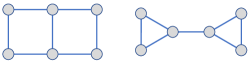
Strict sepatation. It is easy to give a pair of counterexample graphs that are indistinguishable by 1-WL but can be distinguished via EPWL. We give such a pair of graphs in Figure 2. One can check that the two graphs has difference set of eigenvalues no matter what graph matrix is used in EPWL.
We next show that EPWL is more expressive than spectral positional encoding using Laplacian eigenvectors. We will prove the following result:
Proposition A.6.
Given any graph matrix and any initial color mapping , let be the EPWL color mapping after the first iteration. Then, for any graphs and vertices , if , then .
Proof.
Let and vertices satisfy that . Then,
| (13) |
Note that for any and , if , then (Lemma A.5). Therefore, Equation 13 implies that . ∎
A.3 Proof of Theorem 4.3
This subsection aims to prove Theorem 4.3. We will first restate Theorem 4.3 using the color refinement terminologies defined in Section A.1. We need the following color transformations:
-
•
EPWL color refinement. Define such that for any color mapping and rooted graph ,
(14) -
•
SWL color refinement. Define such that for any color mapping and rooted graph ,
(15) -
•
PSWL color refinement. Define such that for any color mapping and rooted graph ,
(16) -
•
Global refinement. Define such that for any color mapping and rooted graph ,
(17) (18) -
•
Diagonal refinement. Define such that for any color mapping and rooted graph ,
(19) (20) -
•
Node marking refinement. Define such that for any color mapping and rooted graph ,
(21) -
•
Lift transformation. Define such that for any color mapping and rooted graph ,
(22) -
•
Subgraph pooling. Define such that for any color mapping and rooted graph ,
(23) -
•
Global pooling. Define such that for any color mapping and graph ,
(24)
Note that , , and . Equipped with the above color transformations, Theorem 4.3 is equivalent to the following:
Theorem A.7.
For any graph matrix , .
We will decompose the proof into a set of lemmas. First, we leverage a recent breakthrough in graph theory established by Rattan & Seppelt (2023). We restate their result in our context as follows.
Definition A.8.
Define a family of graph matrices as follows, called equitable matrices:
-
a)
Base matrices: the identify matrix , all-one matrix , adjacency matrix , degree matrix are all equitable;
-
b)
Algebraic property: for any equitable matrices , , where can be any constant.
-
c)
Spectral property: for any and , let be the projection onto the eigenspace spanned by the eigenvectors of with eigenvalue ( if is not an eigenvalue of ). Then, .
Based on Definition A.8, we readily have the following proposition:
Proposition A.9.
The Laplacian matrix and the normalized Laplacian matrix are equitable.
Rattan & Seppelt (2023) proved the following main result:
Theorem A.10.
For any , , where is the constant color mapping.
Corollary A.11.
For any symmetric equitable matrix and initial color mapping , .
Proof.
For any symmetric equitable matrix and any , holds by Definition A.8(c). Therefore, Theorem A.10 implies that , i.e., . Next, note that iff is an eigenvalue of . Therefore, the graph invariant over defined by satisfies that . Since (based on the facts and and Corollary A.3), we have . By considering all , we obtain that . Finally, noting that is order-preserving and , we have for all . ∎
We are now ready to prove Theorem A.7.
Proof of Theorem A.7.
Note that is a color refinement, and thus . To prove that , it suffices to prove that according to Proposition A.1. Moreover, based on Proposition A.2, it suffices to prove that .
Let be any initial color mapping and let . Pick any graphs and vertices such that , i.e.,
| (25) |
Invoking Corollary A.11 obtains that
| (26) |
Since , based on Corollary A.3 we have , i.e., . Therefore,
| (27) |
Since , we similarly have . Therefore,
| (28) |
Combining with Equations 25 and 28, we have . Finally, noting that is arbitrary, we conclude that . ∎
A.4 Proof of Theorem 5.1
This subsection aims to prove Theorem 5.1. We will first restate Theorem 5.1 using the color refinement terminologies defined in Section A.1. Similarly to Section A.3, we define the following color transformations:
-
•
EPWL color refinement. Define such that for any color mapping and rooted graph ,
(29) -
•
GD-WL color refinement. Define such that for any color mapping and rooted graph ,
(30) -
•
Global pooling. Define such that for any color mapping and graph ,
(31)
Theorem 5.1 is equivalent to the following:
Theorem A.12.
For any graph distance matrix listed in Section 5, .
In this subsection, let be the constant color mapping and let . Define a color mapping such that for all graph and vertices . The following proposition will play a central role in our subsequent proofs:
Proposition A.13.
For any graph matrix , if , then .
Proof.
Based on Propositions A.1 and A.2, it suffices to prove that . Pick any and let . Since , we have
for all graphs and vertices . Moreover, since and , we have
for all graphs and vertices . Therefore, . Finally, by noting that and is arbitrary, we obtain that , as desired. ∎
We next present several basic facts about EP-WL stable colors .
Proposition A.14.
For any graphs and vertices , if , then
-
a)
;
-
b)
.
Proof.
Since (Lemma A.5), we have . Item (a) follows from the fact that the 1-WL stable color can encode the vertex degree, i.e., . To prove item (b), note that , where is defined in Proposition A.6. Therefore, item (b) readily follows from Proposition A.6. ∎
Below, we will separately consider each of the distances listed in Section 5.
Lemma A.15.
Let be the shortest path distance matrix. Then, .
Proof.
We will prove a stronger result that . Note that there is a relation between and the normalized adjacency matrix , which can be expressed as follows:
| (32) |
The above relation can be interpreted as follows: where ranges over all walks of length from to , and for a walk , which is always positive.
Based on the property of eigen-decomposition, we have
| (33) |
This implies that can be purely determined by , i.e., . ∎
Lemma A.16.
Let be the resistance distance matrix. Then, .
Proof.
We first consider the case of connected graphs. We leverage a celebrated result established in Klein & Randic (1993), which builds connections between resistance distance and graph Laplacian. Specifically, for any connected graph and vertices ,
| (34) |
where denotes the matrix Moore–Penrose inversion. Substituting into Equation 34, we obtain
| (35) |
Moreover, we have where is the eigen-decomposition of . Combining all these relations, one can see that is purely determined by the tuple . Based on Proposition A.14, determines and , and determines and . Consequently, .
We next consider the general case where the graph is disconnected. In this case, is a block diagonal matrix. It is straightforward to see that
| (36) |
Since we have proved that can encode the shortest path distance (Lemma A.15), can encode whether and are in the same connected component. So we still have . ∎
Lemma A.17.
Let be the hitting-time distance matrix. Then, .
Proof.
Without loss of generality, we only consider connected graphs as in Lemma A.16. According to the definition of hitting-time distance, for any connected graph and vertices , we have the following recursive relation:
| (37) |
Now define a new graph matrix
| (38) |
where is the diagonal matrix obtained from by zeroing out all non-diagonal elements of . It follows that .
We first calculate . Left-multiplying Equation 38 by yields that
where we use the fact that . Therefore, , namely, .
We next compute the full matrix . Based on Equation 38, we have
| (39) |
Left-multiplying Equation 39 by leads to the fundamental equation
| (40) |
When the graph is connected, the eigenspace of associated with eigenvalue only has one dimension, and any eigenvector satisfying has the form for some . This implies that all solutions to Equation 40 has the form
| (41) |
where is a diagonal matrix and . Noting that , we have . Since for any diagonal matrix and , we final obtain
| (42) | ||||
Below, we will prove that . Noting that , we have
| (43) |
Equivalently, for any graph and vertices ,
| (44) | ||||
From the above equation, one can see that is fully determined by the following tuple:
According to the eigen-decomposition, where is the eigen-decomposition of . Therefore, . Besides, based on Proposition A.14 we have that is determined by , is determined by , and is determined by . It follows that is determined by , because by we have for all graphs and vertices ,
We next prove that is determined by . Again by using , we have for all graphs and vertices ,
Using the same analysis and noting that for any symmetric matrix , we can prove that is determined by . Combining all these relations leads to the conclusion that . ∎
Corollary A.18.
Let be the commute-time distance matrix. Then, .
Proof.
This is a simple consequence of Lemma A.17. Denoting by the hitting-time distance matrix, we have . Since , (because for any graph and vertices ). Therefore, . ∎
Lemma A.19.
Let be the PageRank distance matrix associated with weight sequence . Then, .
Proof.
By definition of PageRank distance, . Let be the eigen-decomposition of . Then, . Therefore,
| (45) |
Plugging the above equation into the definition of PageRank distance, we have for any graph and vertices ,
| (46) |
One can see that is purely determined by the tuple . Based on Proposition A.14, determines and determines . Consequently, . ∎
We next study the (normalized) diffusion distance. Consider the continuous graph diffusion process defined as follows. Given time , let be the probability “mass” of particles at position . The particles will move following the differential equation given below:
| (47) |
where is the transition matrix. For example, when , the differential equation essentially characterizes a random walk diffusion process. In this paper, we consider the normalized diffusion distance, which corresponds to . Given hyperparameter , denote by be the probability “mass” vector at time with the initial configuration and for all . Then, the diffusion distance matrix is defined as
| (48) |
Lemma A.20.
Let be the normalized diffusion distance defined above. Then, .
Proof.
Since Equation 47 is a linear differential equation, we can solve it and obtain . Therefore,
| (49) |
where is the matrix exponential of . Equivalently,
| (50) |
Let be the eigen-decomposition of . Then, . Therefore,
| (51) |
This implies that is purely determined by the tuple . We conclude that by using Proposition A.14. ∎
We finally study the biharmonic distance.
Lemma A.21.
Let be the biharmonic distance defined in Lipman et al. (2010). Then, .
Proof.
Without loss of generality, we only consider connected graphs. According to Wei et al. (2021), the biharmonic distance for a connected graph can be equivalently written as
| (52) |
The subsequent proof is almost the same as in Lemma A.16 and we omit it for clarity. ∎
A.5 Proof of Theorem 6.1
This section aims to prove Theorem 6.1. Below, we will decompose the proof into three parts. First, we will describe the color refinement algorithm corresponding to Spectral IGN, which is equivalent to Spectral IGN in terms of distinguishing non-isomorphic graphs. Then, we will prove that this color refinement algorithm is more expressive than EPWL using the color refinement terminologies defined in Section A.1. Finally, we will prove the other direction, i.e., EPWL is more expressive than the color refinement algorithm of Spectral IGN, thus concluding the proof of Theorem 6.1.
Color refinement algorithm for Spectral IGN. To define the algorithm, we first need to extend several concepts defined in Section A.1 to incorporate eigenvalues. Formally, let be the graph spectrum invariant representing the set of eigenvalues for graph matrix , i.e., for . Define
| (53) |
We can then define color mappings over . Formally, a function defined over domain is called a color mapping if holds for all satisfying and . Without ambiguity, we will use the notation to refer to for . Define to be the family of all color mappings over . We can similarly define equivalence relation “” and partial relation “” between color mappings in . In addition, the color transformation can also be extended in a similar manner.
Throughout this section, we use the notation to represent the initial color mapping in Spectral IGN, which is defined as for all , where is the projection matrix associated with eigenvalue . We then define the following color transformations:
-
•
2-IGN color refinement. Define such that for any color mapping and ,
(54) Here, the function satisfies that if and otherwise (0 is a special element that differs from all ). One can see that Equation 54 has 15 aggregations inside the hash function, which matches the number of orthogonal bases for a 2-IGN layer (Maron et al., 2019b).
-
•
Spectral pooling. Define such that for any color mapping and ,
(55) -
•
Spectral IGN color refinement. Define such that for any color mapping and ,
(56) -
•
Spectral IGN final pooling. Define such that for any color mapping and ,
(57) -
•
Joint pooling. Define such that for any color mapping and ,
(58) -
•
2-dimensional Pooling. Define such that for any color mapping and ,
(59) -
•
EPWL color refinement. Define such that for any color mapping and ,
(60) -
•
Global pooling. Define such that for any color mapping and graph ,
(61)
We now related the expressive power of Spectral IGN to the corresponding color refinement algorithm. The proof is straightforward following standard techniques, see e.g., Zhang et al. (2023a).
Proposition A.22.
The expressive power of Spectral IGN is bounded by the color mapping in distinguishing non-isomorphic graphs. Moreover, with sufficient layers and proper network parameters, Spectral IGN can be as expressive as the above color mapping in distinguishing non-isomorphic graphs.
Equivalently, the pooling can be decomposed into three pooling transformations , as stated below:
Lemma A.23.
.
Proof.
First, it is clear that . Thus, it suffices to prove that . Pick any initial color mapping and let . Note that . We will prove that . Pick any graphs . We have
where the second, third, and fourth steps in the above derivation are based on Equations 54, 55 and 56. We have obtained the desired result. ∎
In the subsequent proof, we will show that , where is the constant mapping.
Lemma A.24.
Let be the constant mapping. Then, .
Proof.
Define an auxiliary color transformation such that for any color mapping and rooted graph ,
| (62) |
We first prove that . Pick any color mapping and graphs ,
Based on the equivalence, it suffices to prove that . Since is order-preserving by definition, it suffices to prove that .
We will prove the following stronger result: for all , . The proof is based on induction. For the base case of , since is a constant mapping, the result clearly holds. Now assume that the result holds for and consider the case of . Denote , , and note that . Pick any graphs and vertices , . Based on the induction hypothesis, implies that and . We have
where in the first step we use the definition of Spectral IGN (Equation 56) and spectral pooling (Equation 55); in the third step we use the definition of 2-IGN (Equation 54); in the fourth step we use the induction hypothesis and the fact that . This concludes the induction step. ∎
Lemma A.25.
Define an auxiliary color transformation such that for any color mapping and rooted graph ,
| (63) |
Then, .
Proof.
We will prove the following stronger result: for any , . The proof is based on induction. For the base case of , since , the result clearly holds. Now assume that the result holds for and consider the case of . Denote and . Pick any graphs and vertices , . Based on the induction hypothesis, implies that . We have
where in the second step we use the definition of and also Lemmas A.5 and A.6; in the third step we use the definition of again; in the fourth step we use the induction hypothesis and the fact that for all and ; in the last step we use the definition of 2-IGN (Equation 54).
We next prove that . This is because
where in the first step we use the following observations: , which implies that ; and thus . We thus conclude the induction step. ∎
Lemma A.26.
Let be the constant mapping. Then, .
Proof.
Based on Lemma A.25, it suffices to prove that , where is defined in Lemma A.25. Denote . Let be any graphs such that . By definition of ,
| (64) |
Since ,
| (65) |
Equivalently,
| (66) |
This implies that , concluding the proof. ∎
Combining Propositions A.22, A.23, A.24 and A.26, we conclude the proof of Theorem 6.1.
A.6 Proof of Propositions 6.3 and 6.5
This sections aims to prove Propositions 6.3 and 6.5. We will first give a brief introduction of BasisNet. The BasisNet architecture is composed of two parts: an eigenspace encoder and a top graph encoder . Here, we consider the standard setting where is a messgage-passing GNN that takes node features as inputs and outputs a graph representation invariant to node permutation. We assume that the expressive power of is bounded by the classic 1-WL test.
We next describe the design of the eigenspace encoder . Given graph matrix and graph , let be the eigen-decomposition of , where are eigenvalues of . For each eigenspace, BasisNet processes the projection matrix using a 2-IGN , where is the multiplicity of eigenvalue . The output of is then defined as
| (67) |
where denotes the concatenation. When the number of eigenspaces is less than the output dimension , zero-padding is applied. Note that BasisNet processes different projections using different IGNs if their multiplicities differ.
Color refinement algorithms for Siamese IGN and BasisNet. Similar to Spectral IGN, we can write the corresponding color refinement algorithms for the two GNN architectures. We first define the initial color mapping as follows: for all , where is the projection matrix associated with eigenvalue and is the multiplicity of eigenvalue . Here, we encode the multiplicity in because BasisNet uses different IGNs for different eigenvalue multiplicities. We then define several color transformations:
-
•
Siamese IGN color refinement. Define such that for any color mapping and ,
(68) where is defined in Equation 54.
-
•
BasisNet pooling. Define such that for any color mapping and ,
(69) One can see that Equation 69 has 5 aggregations inside the hash function, which matches the number of orthogonal bases in Maron et al. (2019b).
-
•
Spectral pooling. Define such that for any color mapping and ,
(70) Similarly, define such that for any color mapping and ,
(71) -
•
Joint pooling. This has been defined in Equation 58.
-
•
Diagonal pooling. Define such that for any color mapping and rooted graph ,
(72) -
•
1-WL refinement. This has been defined in Equation 11.
-
•
Global pooling. This has been defined in Equation 61.
We are ready to define the color mappings corresponding to the whole algorithms:
-
•
Weak Spectral IGN: the color mapping is defined as .
-
•
BasisNet: the color mapping is defined as .
Similar to the previous analysis, we can prove that the above two color mappings upper bound the expressive power of the corresponding GNN models. Below, it suffices to prove the following key lemma:
Lemma A.27.
For any graph matrix , .
Proof.
The proof will be decomposed into a series of steps. We first prove that . It suffices to prove that . Pick any graphs , eigenvalues , and vertices , . Then, by definition of , implies that
| (73) |
Therefore, , where denotes the matrix trace. Noting that is exactly the multiplicity of eigenvalue for graph matrix , we have .
We then prove that . Pick any initial color mapping and let . Note that . We will prove that . Pick any graphs . We have
where the second step is based on Lemma A.5, and the third step is based on the definition of . This proves that .
We next prove that . Pick any graphs and vertices , . We have
where the second step is based on the definition of . This proves that .
We conclude the proof by combining the above relations with Propositions A.1 and A.2. ∎
We next turn to the proof of Proposition 6.5, which is almost the same as the case of BasisNet. Below, we will define the equivalent color refinement algorithm for SPE. The initial color mapping associated with SPE is simply . Then, the architecture refines by using color transformation defined in Equation 54. The remaining procedure is the same as BasisNet. Combined these together, the color mapping corresponding to the whole algorithm can be written as . Then, it suffices to prove the following two equivalence relations: ; . The proof procedure is alomst the same as in Sections A.5 and A.6 and we omit it here.
A.7 Discussions with other architectures
Graphormer (Ying et al., 2021), Graphormer-GD (Zhang et al., 2023b), and GraphiT (Mialon et al., 2021). Zhang et al. (2023b) has shown that the expressive power of these architectures is inherently bounded by GD-WL with different distances. Here, Graphormer uses SPD, Graphormer-GD uses both SPD and RD, while the distance used in GraphiT has the form , where is the projection matrix associated with eigenvalue for graph matrix , and is a general function. Therefore, based on Theorem 5.1 and the proof, it is straightforward to see that all these architectures are bounded by EPWL.
PEG (Wang et al., 2022). Given graph , PEG maintains a feature vector for each node in each layer , and the feature is updated by the following formula:
| (74) |
where and are arbitrary functions, is a parameterized weight matrix, and is the positional encoding corresponding to the top eigenvectors at node . Here, we assume that the number is chosen such that is unique for all graphs of interest (i.e., no ambiguity problem).
We will show that the expressive power of PEG is bounded by EPWL. To obtain this result, note that . Since is unique, the span of top eigenvectors must be equivalent to the direct sum of the eigenspaces corresponding to top eigenvalues for some . It follows that where is the projection onto the eigenspace corresponding to eigenvalue . Therefore, the expressive power of PEG is bounded by the color refinement algorithm with the initial color mapping and the color transformation defined below:
| (75) |
We will prove that . Based on Propositions A.1 and A.2, it suffices to prove that . Denote and note that . Pick any graphs and vertices , . We have
where in the first and second steps we use Proposition A.14. This concludes the proof that the expressive power of PEG is bounded by EPWL.
GIRT (Ma et al., 2023b). Given graph , GIRT maintains a feature vector for both vertices and vertex pairs. Denote by the feature of node in layer , and denote by the feature of node pair in layer . The features are updated by the following formula:
| (76) | |||
| (77) | |||
| (78) |
where the initial feature is defined as
One can easily write the corresponding color refinement algorithm that upper bounds of the expressive power of GIRT. Formally, it can be expressed as , where is defined in Equation 72, the initial color mapping is simply the multi-dimensional PageRank distance, and is the color refinement defined below:
| (79) |
We will prove that . Define color transformation such that for any color mapping and rooted graph ,
| (80) |
Note that by Proposition A.14. Also, due to Lemma A.16. Therefore, it suffices to prove that . Based on Proposition A.2, it suffices to prove that . Denote , where is any initial color mapping. Pick any graphs and vertices , such that . We have:
-
•
If , then .
-
•
If , then .
Here, in the above derivations we use Proposition A.14. We have concluded the proof that the expressive power of GIRT is bounded by EPWL.
Spectral PPGN and Spectral -IGN. Based on Maron et al. (2019a), PPGN can mimic the 2-FWL test (Cai et al., 1992), and Spectral -IGN can mimic the -WL test (Grohe, 2017). Let and be the color refinements associated with -WL and -FWL, respectively, and let be the initial color mapping in -WL and -FWL. The color refinement algorithms corresponding to -WL and -FWL can then be described as and , respectively, where is defined in Equation 84. Maron et al. (2019a) proved that with sufficiently layers, the features of vertex -tuples computed by -IGN is finer than , and the features of vertex pairs computed by PPGN is finer than . Later, Azizian et al. (2021) proved that the features of vertex pairs computed by PPGN is also bounded by (and thus as fine as) (see Lemma 12 in their paper). Finally, Geerts & Reutter (2022) proved that the features of vertex -tuples computed by -IGN is bounded by (and thus as fine as) (see Lemma E.1 in their paper).
We now define the color refinement algorithms for Spectral PPGN and Spectral -IGN, which are as expressive as the corresponding GNN architectures based on the results of Maron et al. (2019a); Azizian et al. (2021); Geerts & Reutter (2022). First define the following color transformations:
-
•
Spectral -IGN color refinement. Define such that for any color mapping and ,
(81) -
•
Spectral PPGN color refinement. Define such that for any color mapping and ,
(82) -
•
Spectral pooling. Define such that for any color mapping and ,
(83) -
•
Joint pooling. Define such that for any color mapping and ,
(84)
Define the initial color mapping such that for any graph , vertices , and ,
| (85) |
where is the projection onto eigenspace associated with eigenvalue for graph matrix . The color refinement algorithm for Spectral PPGN is then defined as . Similarly, the color refinement algorithm for Spectral -IGN is then defined as . We aim to prove that following two results:
Proposition A.28.
.
Proposition A.29.
.
We will only prove Proposition A.28, as the proof of Proposition A.29 is almost the same.
Proof of Proposition A.28.
We first prove that . Since (Lemma A.5), it suffices to prove that . Based on Proposition A.2, it suffices to prove that . Denote , where is any initial color mapping. Pick any graphs and vertices , such that . We have:
where in the second step we use the definition of and the fact that .
We next prove that . Based on Zhang et al. (2023a), we have and , where , are defined in Section A.3. On the other hand, we have proved in Corollary A.11 that . Therefore, . This finally implies that .
It thus suffices to prove that . We will prove the following stronger result: for any , . The proof is based on induction. For the base case of , the result clearly holds. Now assume that the result holds for and consider the case of . Denote . Pick any graphs and vertices , . We have
Combining the last two steps implies that . We thus conclude the induction step. ∎
A.8 Counterexamples
In this subsection, we aim to reveal the expressivity gaps between different GNN models. This is achieved by constructing a pair of counterexample graphs such that one GNN can distinguish while the other cannot. Here, we will leverage an important theoretical tool to construct counterexamples, known as Fürer graphs Fürer (2001). An in-depth introduction of Fürer graphs can be found in Zhang et al. (2023a).
Definition A.30 (Fürer graphs).
Given any connected graph , the Fürer graph is constructed as follows:
Here, holds when either ( and ) or ( and ) holds. For each , denote the set
| (86) |
which is called the meta vertices of associated to . Note that .
We next define an operation called “twist”:
Definition A.31 (Twisted Fürer graphs).
Let be the Fürer graph of , and let be an edge of . The twisted Fürer graph of for edge , is constructed as follows: , where
and is the symmetric difference operator, i.e., . For an edge set , we further define
| (87) |
Note that Equation 87 is well-defined as the resulting graph does not depend on the order of edges for twisting.
The following result is well-known (see e.g., Zhang et al., 2023a, Corollary I.5 and Lemma I.7)):
Theorem A.32.
For any graph and any set , iff .
Below, we will prove Proposition A.33 using Fürer graphs. Note that it can be easily checked via a computer program whether a pair of graphs can be distinguished by a given color refinement algorithm. However, an in-depth understanding of why a given color refinement algorithm can/cannot distinguish these (twisted) Fürer graphs is beyond the scope of this paper and is left for future work.
Proposition A.33.
The following hold:
-
a)
There exists a pair of graphs such that SWL cannot distinguish them but Siamese IGN, Spectral IGN, and EPWL with any graph matrix can distinguish them;
-
b)
For any , there exists a pair of graphs such that Weak Spectral IGN cannot distinguish them but Spectral IGN can distinguish them;
-
c)
There exists a pair of graphs such that Weak Spectral IGN cannot distinguish them with any , but GD-WL with any distance listed in Section 5 can distinguish them;
-
d)
There exists a pair of graphs such that Spectral IGN and EPWL with any graph matrix cannot distinguish them, but SWL can distinguish them;
-
e)
There exists a pair of graphs such that Siamese IGN with any graph matrix cannot distinguish them, but Weak Spectral IGN with any graph matrix can distinguish them.
| (a) | (b) | (c) | (d) | (e) |
Proof.
For Proposition A.33(a,b,c,d,e), the counterexample graphs are the Fürer graph and twisted Fürer graph for base graph defined in Figure 3(a,b,c,d,e), respectively. ∎