Coarse-To-Fine Tensor Trains for Compact Visual Representations

Abstract

The ability to learn compact, high-quality, and easy-to-optimize representations for visual data is paramount to many applications such as novel view synthesis and 3D reconstruction. Recent work has shown substantial success in using tensor networks to design such compact and high-quality representations. However, the ability to optimize tensor-based representations, and in particular, the highly compact tensor train representation, is still lacking. This has prevented practitioners from deploying the full potential of tensor networks for visual data. To this end, we propose ‘Prolongation Upsampling Tensor Train (PuTT)’, a novel method for learning tensor train representations in a coarse-to-fine manner. Our method involves the prolonging or ‘upsampling’ of a learned tensor train representation, creating a sequence of ‘coarse-to-fine’ tensor trains that are incrementally refined. We evaluate our representation along three axes: (1). compression, (2). denoising capability, and (3). image completion capability. To assess these axes, we consider the tasks of image fitting, 3D fitting, and novel view synthesis, where our method shows an improved performance compared to state-of-the-art tensor-based methods.

https://github.com/sebulo/PuTT

1 Introduction

Building a compact, easy-to-fit, and high-quality visual data representation is paramount for many computer vision and graphics applications, such as novel view synthesis, 3D fitting, and generation (Xie et al., 2022). To this end, recent research within neural field representations (Chen et al., 2022; Obukhov et al., 2022; Müller et al., 2022) has directed its focus towards the sparsity and efficiency of tensor networks, hinting at the potential gains in the compactness and quality of such representations. In particular, TensoRF (Chen et al., 2022) applied low-rank tensor decomposition of radiance fields to achieve substantial efficiency gains. This approach was further extended by TT-NF (Obukhov et al., 2022), which utilized a tensor train representation to improve compression. Indeed, tensor trains, as well as more complex tensor networks (Orús, 2014; Vidal, 2007), are known to allow substantial improvements in compression.

However, despite encouraging progress, the full realization of tensor networks for compact and efficient representations is still lacking. The main obstacles of current tensor-based representations are: (1). Optimization using current gradient-based schemes often gets stuck in local minima and falls short of the ultimate compression limit of the tensor train format. In particular, TensoRF (Chen et al., 2022) can only handle small tensors and does not enjoy the significant parameter efficiency of tensor trains. TT-NF (Obukhov et al., 2022) highlights the capacity of tensor trains to model larger tensors using significantly fewer parameters compared to TensoRF, offering, in principle, a more scalable approach. However, TT-NF lacks efficient optimization strategies aligned to TensoRF. TT-NF often reaches a local minimum in optimization and cannot model the full potential of tensor trains, resulting in poorer performance. (2). They often struggle with noisy and incomplete data.

Toward resolving these obstacles, we propose a novel, coarse-to-fine, tensor-train-based representation called ‘Prolongation Upsampling Tensor Train (PuTT)’ and an associated gradient-based optimization strategy. Our strategy involves the prolonging or ‘upsampling’ of a learned tensor train representation in a coarse-to-fine manner, creating a sequence of ‘coarse-to-fine’ tensor trains that are incrementally refined. The coarse-to-fine operations are performed directly in the tensor train format, circumventing the need to process individual data points, as is customary in linear interpolation. This allows for efficient sampling and for PuTT to be applied to extremely fine grids and to fit high-resolution data at limited additional memory and computational cost.

Central to PuTT is its unique capability to learn Quantized Tensor Trains (QTT) (Oseledets, 2009), a tensor format designed for efficient representation through hierarchical structuring. It does so through a hierarchical refinement process, reminiscent of the multigrid method for solving partial differential equations (Bramble, 2019). Our iterative coarse-to-fine representation and optimization strategy enables significant parameter efficiency of tensor trains on the one hand and their efficient optimization on the other. The empirical findings indicate that our strategy effectively mitigates the impact of local minima during training, thereby enabling a parametrized learning model to approach the theoretical limit allowed within the TT format; as obtained by the TT-SVD decomposition (Oseledets, 2011). Unlike TT-SVD, our strategy employs learning from samples, and benefits from the associated versatility.

Visual data is known to have a natural hierarchical structure, as evidenced by the success of wavelet-based methods in image and video compression (Antonini et al., 1990). To this end, the adoption of QTT in PuTT is motivated by its suitability for handling the multi-resolution nature and dependencies within subregions of data, akin to those in visual data. Compared to other tensor decompositions like CP and Tucker, which scale linearly with dimension (d) and side length (L), QTT offers a more modest scaling in side length $\mathcal{O}(d\log(L)R^{2})$, where $R$ is the rank and captures the correlation in the data across dimensions and resolution scale. This scalability positions QTT as an effective choice for large-scale tensors, surpassing CP, VM, and Tucker in space efficiency, which is especially beneficial as dimensions and resolutions increase. We evaluate our representation along three axes: (1). compression, (2). denoising capability, and (3). ability to learn from incomplete or missing data. To value these axes, we consider the tasks of image fitting, 3D fitting, and novel view synthesis, where our method shows improved qualitative and quantitative performance compared to state-of-the-art tensor-based baselines.

2 Related Work

Coarse-to-Fine Representations  Coarse-to-fine, or multi-scale, visual representations were developed for several purposes, such as compression or reducing transmission time (Szeliski, 2022). Early works include multi-resolution pyramids such as Laplacian and Gaussian pyramids (Adelson et al., 1984), half-octave pyramids (Crowley & Stern, 1984) and wavelets (Mallat, 1989). Recently, coarse-to-fine representations were used to build neural fields (Yang et al., 2022; Lindell et al., 2022). Similarly, Instant-NGP (Müller et al., 2022) uses a learned mutual-resolution grid representation as a fast and compact representation for novel view synthesis. Similarly to our method, this representation is learned using SGD. Our method, however, considers a more general and compact learned multi-scale representation, whereby the hierarchy levels are tensor trains.

Compact Visual Representations  Visual representations can be divided between explicit, implicit, and hybrid representations. Explicit representations, such as image grids, 3D meshes, point clouds and voxel grids are interpretable and expressive but expensive to store and scale. Implicit representations (Sitzmann et al., 2019; Lombardi et al., 2019) were used for applications such as novel view synthesis (Müller et al., 2022), generative modeling (Niemeyer & Geiger, 2021; Chan et al., 2021, 2022), and surface reconstruction (Oechsle et al., 2021). While compact, they are known to be slow. To this end, hybrid representations were developed. For instance, DVGO (Sun et al., 2022) optimize voxel grids of features. This leads to significantly lower memory and capacity requirements. Instant-NGP (Müller et al., 2022) combines an explicit multi-resolution hashable feature grid with small MLP mapping features to color and opacity values. While our approach also employs a multiresolution structure, it is centered around a factorization of a quantized hierarchical structure in each layer. Hashing is an orthogonal technique; combining it with our method is left for future work.

Tensor network representations  Large-scale tensor networks have seen extensive applications in quantum physics (White, 1992b), including quantum computation (Pan & Zhang, 2022), and can be used to simulate strongly correlated systems (Orús, 2019). To learn visual representations, TensoRF (Chen et al., 2022) significantly improved compression by using CP and VM decomposition for NeRFs. CP decomposition was later extended by (Liu et al., 2020b). Instead, our method can handle a much more expressive representation of tensor trains. Our method extends the potential of tensor trains for larger tensors, as noted in TT-NF (Obukhov et al., 2022), by incorporating a coarse-to-fine approach that ensures efficient optimization similar to TensoRF and enhances denoising and image completion capabilities. This strategy helps to fully utilize the expressive strength of tensor-train representations.

3 Notation

Graphical notation  Tensor Network Notation (TNN) provides a powerful tool for visualizing the interactions between tensors in a tensor network. In these visualizations (diagrams), each tensor is represented as a node, with a number of legs corresponding to its dimensions. For example: (i). A matrix $W\in\mathbb{R}^{m\times n}$ is as a node with two legs: . (ii). A vector $x\in\mathbb{R}^{n}$ is a node with a single leg: . (iii). Vector-matrix multiplication $Wx$ is depicted by contracting (summing over) legs of the connected tensors: . (iv). Larger tensors $T\in\mathbb{R}^{m\times n\times r}$ have more legs: .

Such diagrams, composed of nodes and their interconnections, effectively depict what is known as a “tensor network”. We focus on four classes of tensor networks: the CP, Tucker, and tensor train decompositions. In 3D, we also consider the VM construction (Chen et al., 2022). For discussion and details on these tensor networks, see the appendix.

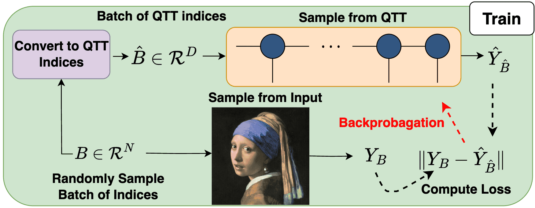
Figure 1: Training one level of hierarchy. Initially, a batch $B$ serves two purposes: (1). sample data points $Y_{B}$ from the target input, (2). it is transformed into QTT indices $\hat{B}$. Subsequently, corresponding values $\hat{Y}_{\hat{B}}$ are sampled from the QTT. The reconstruction loss between $Y_{B}$ and $\hat{Y}_{\hat{B}}$ is used and backpropagated.

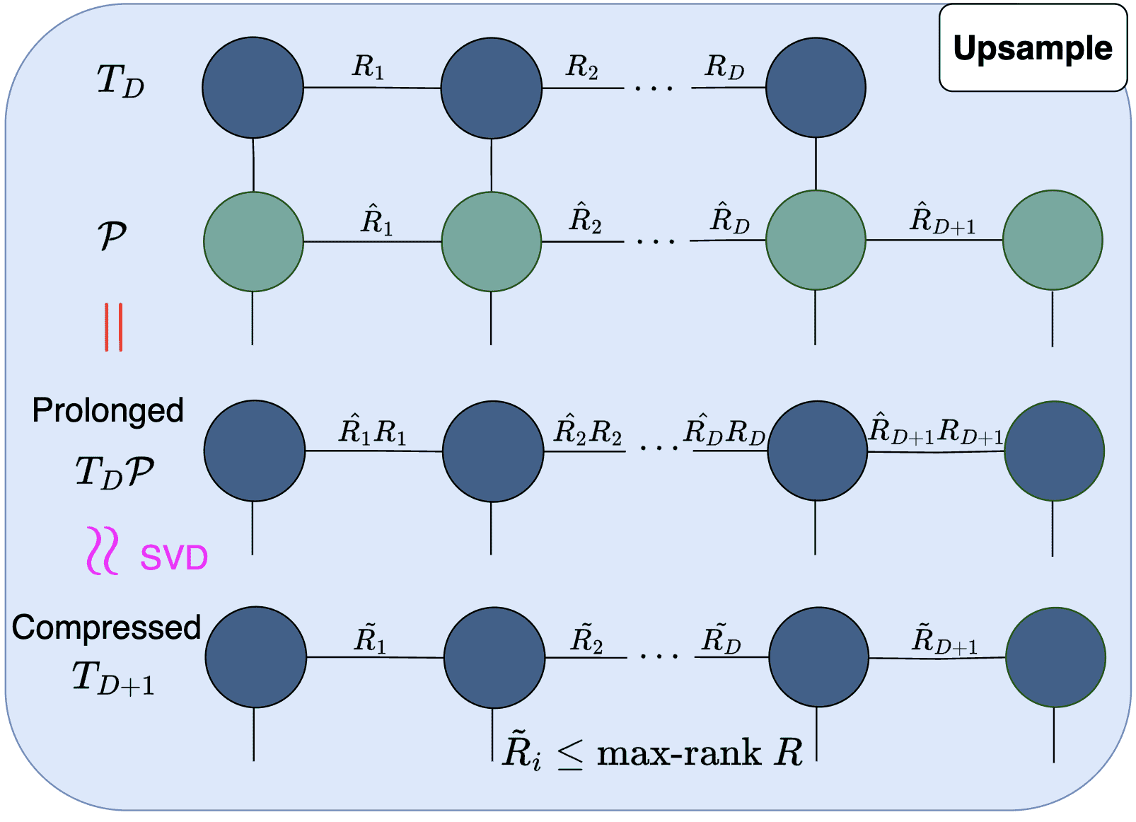
Figure 2: Illustration of QTT upsampling process. Beginning with a QTT $T_{D}$ of length $D$, upsampling is achieved through the prolongation MPO $\mathcal{P}$. This involves connecting the $D+1$ cores of $\mathcal{P}$ to the corresponding cores of $T_{D}$ and then contracting their shared indices. The result is a new QTT, $T_{D+1}$, of length $D+1$, where ranks are increased to $R_{i}\hat{R}_{i}$. To manage this rank growth, TT-SVD (Oseledets, 2011) is employed for rank truncation. This process yields $T_{D+1}$ with controlled ranks $\tilde{R}_{i}\leq R_{max}$.

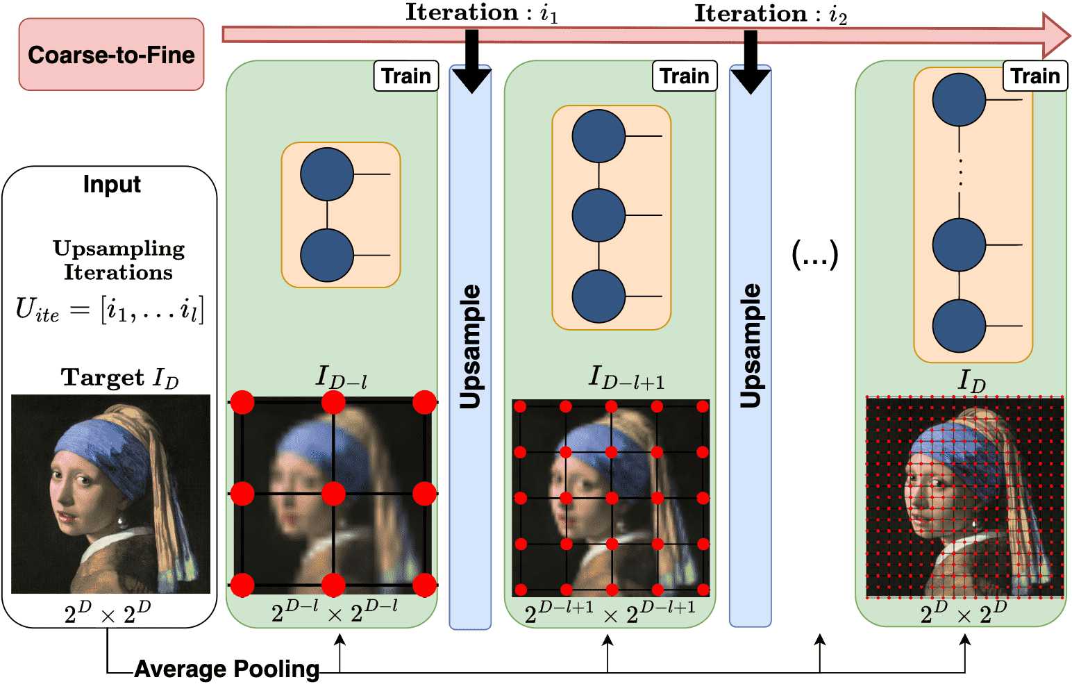
Figure 3: Full coarse-to-fine learning, integrating ‘Train’ and ‘Upsample’ phases of Fig.1 and Fig.2. We start with input $I_{D}$, which is downscaled to $I_{D-l}$ (resolution $2^{d-l}\times 2^{d-l}$). A QTT is then randomly initialized for $I_{D-l}$. After training this QTT (as per Fig.1) up to iteration $i_{1}$, we proceed with upsampling (as illustrated in Fig. 2), producing $T_{D-l+1}$ of length $D-l+1$. This represents a grid at resolution $2^{d-l+1}\times 2^{d-l+1}$ and requires sampling from a newly downsampled target $I_{D-l+1}$ of the same resolution.

Tensor Train (Oseledets, 2011) or a Matrix Product State (MPS) (Klümper et al., 1993; Perez-Garcia et al., 2007), is a decomposition of a tensor with $N$ indices into a chain-like network of $N$ order-$3$ tensors: This structure can be graphically represented in Tensor Network Notation: . Given a tensor $T\in\mathbb{R}^{n_{1}\times n_{2}\times\cdots n_{d}}$, the entries of the tensor are:

$$T_{j_{1}\cdots j_{d}}=A^{j_{1}}A^{j_{2}}\cdots A^{j_{d}},$$ (1)

where $\{A^{j_{k}}\}_{j_{k}=1}^{n_{k}}$ are $R_{j_{k}}\times R_{j_{k+1}}$ matrices for each $j_{k}$; i.e. are $R_{k}\times n_{k}\times R_{k+1}$ tensors. The ranks $R_{k}$ are referred to as the bond dimensions of the tensor train. We distinguish the physical indices $j_{k}$ from the virtual indices $r_{k}$. The bond dimensions $R_{k}$ can be understood as a rank truncation along the cut $n_{1},...,n_{k-1}$ and $n_{k},...,n_{d}$, only keeping the $R$ largest singular values.

In the context of tensor trains, the rank measures the complexity or information content of the tensor. The largest rank among all virtual indices is considered the rank of the tensor train. This rank dictates the ultimate expressivity of the tensor train by determining the number of variational parameters. A tensor $T$ can be represented exactly with a maximal bond dimension $R=\max_{k}\min\{n_{1}\cdots n_{k-1},n_{k}\cdots n_{D}\}$, which scales exponentially in $D$. Tensor trains are used as a parameterized variational class, where we upper bound the bond dimension at some maximal value $R_{\rm max}$. The maximum bond dimension governs the model’s expressivity.

QTT   Compressing visual data along physical dimensions (e.g., image height or width) is natural, as in the CP and Tucker decompositions (Chen et al., 2022). However, significantly more compact representations are possible by compression along the ‘scaling dimension’. For that, we consider the quantized tensor train (QTT) construction (Khoromskij, 2011). The QTT format builds upon mode quantization, which decomposes the scaling dimension in powers of two. As an illustrative example (Obukhov et al., 2022), consider a 3D tensor representing a (regular) function on a $16\times 16\times 16$ lattice. Through mode quantization, this tensor can be recast as a 12-dimensional hypercube: $({\color[rgb]{1,0,0}2_{1}}\times{\color[rgb]{1,0,0}2_{2}}\times{\color[rgb]{1,0,0}2_{3}}\times{\color[rgb]{1,0,0}2_{4}})\times({\color[rgb]{0,1,0}2_{1}}\times{\color[rgb]{0,1,0}2_{2}}\times{\color[rgb]{0,1,0}2_{3}}\times{\color[rgb]{0,1,0}2_{4}})\times({\color[rgb]{0,0,1}2_{1}}\times{\color[rgb]{0,0,1}2_{2}}\times{\color[rgb]{0,0,1}2_{3}}\times{\color[rgb]{0,0,1}2_{4}})$: . In this notation, the subscript indicates levels of hierarchy, and parentheses are used for visual convenience. QTT assumes a particular reordering, where each hierarchical level is grouped as: $({\color[rgb]{1,0,0}2_{1}}\times{\color[rgb]{0,1,0}2_{1}}\times{\color[rgb]{0,0,1}2_{1}})\cdot({\color[rgb]{1,0,0}2_{2}}\times{\color[rgb]{0,1,0}2_{2}}\times{\color[rgb]{0,0,1}2_{2}})\cdot({\color[rgb]{1,0,0}2_{3}}\times{\color[rgb]{0,1,0}2_{3}}\times{\color[rgb]{0,0,1}2_{3}})\cdot({\color[rgb]{1,0,0}2_{4}}\times{\color[rgb]{0,1,0}2_{4}}\times{\color[rgb]{0,0,1}2_{4}})$: . This ordering is far more expressive for hierarchical data, as it avoids bottlenecks connecting low-frequency data in one dimension (say $x$) to high-frequency data in another dimension (say $y$).

Matrix Product operators  A matrix product operator (MPO) is a tensor network that describes a factorization of a tensor with $d$ input and $d$ output indices into a sequence of smaller tensors (Hubig et al., 2017; McCulloch, 2008), with each core having two physical and two virtual indices: . Tensor trains and MPOs differ fundamentally in their applications: Tensor trains serve as compressed representations of large vectors in high-dimensional spaces, while MPOs, denoting matrix-vector operations, act on tensor trains. This distinction enables MPOs to effectively handle large operators within these high-dimensional spaces in a compressed form (Stoudenmire, 2021).

In the appendix, we provide additional details and visualizations of tensor networks. In Sec. D.1, Fig. 16 visualizes the multi-resolution hierarchy of the QTT, illustrating its coarse-to-fine structure. In Sec. D.2, we detail the structure of the specific MPO used for upsampling and the complexity of the prolongation operations.

4 Method

Prolongation operators  While QTT allows for substantial memory savings for equal representational power, it suffers from instabilities in training. Indeed, as observed in (Obukhov et al., 2022; Novikov et al., 2021), without explicit regularization, the QTT representation often fails to improve upon the CP and Tucker representations in practice, getting easily stuck in local minima. To this end, we introduce a global upsampling strategy inspired by the multigrid method for partial differential equations (Bramble, 2019; Lubasch et al., 2018), illustrated in Figs. 1-3 and below.

We use a specific Matrix Product Operator (MPO) – the prolongation operator $\mathcal{P}$ – which performs linear interpolation globally in QTT. Given a vector $v_{n}\in\mathbb{R}^{2^{n}}$ (e.g., a waveform), $\mathcal{P}_{n}$ is a matrix that maps $v_{n}$ to $v_{n+1}\in\mathbb{R}^{2^{n+1}}$, where $v_{n+1}$ is a linear interpolant of $v_{n}$ to a lattice of twice the resolution. $\mathcal{P}_{n}$ is similar to the Haar wavelet transform. Crucially, the matrix $\mathcal{P}_{n}$ is an MPO with a fixed bond dimension of 3. Therefore, it can be applied to a QTT via local tensor operations. The resulting QTT will have (three times) larger bond dimension. If the maximal bond dimension exceeds the desired threshold ($R_{\rm max}$), then the QTT can be compressed down to $R_{\rm max}$ via a local singular value decomposition. For two or three-dimensional visual data, we interpolate in each dimension by applying $\mathcal{P}_{n}\otimes\mathcal{P}_{n}\otimes\mathcal{P}_{n}$.
Fig. 2 demonstrates the application of $\mathcal{P}$ in upsampling a QTT $T_{D}$ of length $D$ to a prolonged QTT, $T_{D+1}$, of length $D+1$. This is achieved by linking $D$ input cores of $\mathcal{P}$ to the corresponding cores of $T$ and contracting the shared indices. As a result, the ranks of $\mathcal{P}T_{D}$ increase, necessitating a rank reduction through TT-SVD (Oseledets, 2011). This reduction is critical since the ranks expand exponentially in the number of upsampling steps. The outcome is a compressed QTT, $T_{D+1}$, with controlled ranks $\tilde{R}_{i}\leq R_{\rm max}$, ensuring an efficient representation of the upsampled object.

4.1 Learning tensor trains (PuTT)

We now outline our Prolongation Upsampling Tensor Train (PuTT) methodology. Training starts at a chosen (coarse) resolution and progressively learns a QTT with finer and finer resolution. Consider a target vector $I_{D}$ representing a visual object of size $(2^{d})^{D}$, where $d$ is the dimension (i.e. $d=2$ for images). We want to learn the best QTT approximation of $I_{D}$, $T_{D}$ with $D$ legs of dimension $2^{d}$ each. We start with a down-sampled object $I_{D-l}$ and learn $T_{D-l}$, where $l$ is the number of upsampling steps. For instance, for an image of resolution $512^{2}$ and three upsampling steps, we start learning $I_{6}$ and upsample three times to reach $I_{9}$.

In our experiments, we learn the QTTs at each resolution via back-propagation, by optimizing the mean squared error. After obtaining a satisfactory approximation of $I_{D-l}$ in QTT format, which we call $T_{D-l}$, we apply the upsampling MPO $\mathcal{P}_{D-l+1}$ to $T_{D-l}$, yielding a QTT with $D-l+1$ ‘physical’ legs $\mathcal{P}_{D-l+1}T_{D-l}$. If the maximal bond dimension exceeds $R_{\rm max}$, then we perform a TT-SVD contraction to keep all ranks below the max $R_{\rm max}$. We then proceed to learn $I_{D-l+1}$ starting from $\mathcal{P}_{D-l+1}T_{D-l}$. Initiating learning with an upsampled prior stabilizes convergence to the correct local or global minimum. The learning proceeds iteratively until we reach the full scale $I_{D}$ and a QTT approximation $T_{D}$. Throughout the learning, we adopt a trapezoid structure (Oseledets, 2011) for the tensor train ranks, where ranks increase to a maximum (forming the trapezoid’s ascending edge), remain constant (trapezoid’s top), and then decrease (its descending edge). The upsampling step of the algorithm is illustrated in Fig. 2, and the full coarse-to-fine learning scheme is illustrated in Fig. 3.

Fig. 1 outlines our training process in a single hierarchy level. Initially, we sample a batch of indices $B$, which serves two purposes: 1. Conversion to a batch of QTT indices $\tilde{B}\in\mathcal{R}^{D}$, mapping cartesian points to QTT points for retrieving values $\hat{Y}_{\hat{B}}$ from the QTT, 2. Using $B$ to sample target input values from $I_{D}$, obtaining $Y_{B}$. These values, $Y_{B}$ and $\hat{Y}_{\hat{B}}$, are used to calculate a mean squared error loss, which is then backpropagated to update the QTT weights.

4.2 Novel View Synthesis

Applying PuTT to novel view synthesis involves modeling a function that maps any 3D location $x$ and viewing direction $d$ to a volume density $\sigma$ and a view-dependent color $c$, supporting differential ray marching for volume rendering (Mildenhall et al., 2020). We use two voxel grids: $\mathcal{G}_{\sigma}$ for volume density and $\mathcal{G}_{c}$ for view-dependent color, similar to TensoRF (Chen et al., 2022). $\mathcal{G}_{\sigma}$ is a single-channel grid encoding $\sigma$ values, while $\mathcal{G}_{c}$ is a multi-dimensional grid holding appearance features. These features are transformed into color values using a shading function $\mathcal{S}$, such as a small MLP or Spherical Harmonics. The continuous grid-based Radiance Field is expressed as:

$$\sigma,c=\mathcal{G}_{\sigma}(x),\mathcal{S}(\mathcal{G}_{c}(x),d)$$

where $\mathcal{G}_{\sigma}(x)$ and $\mathcal{G}_{c}(x)$ are interpolated using trilinear interpolation within the 3D voxel grid.

The tensor representation, $\mathcal{G}_{\sigma}\in\mathbb{R}^{X\times Y\times Z}$, is a 3-order tensor for volume density, and $\mathcal{G}_{c}\in\mathbb{R}^{X\times Y\times Z\times P}$ is a 4-order tensor for color with an additional feature vector dimension $P$. We factorize these grids into QTT-format tensors $T_{\sigma}$ and $T_{c}$, each with $D$ cores and eight physical indices per core, using the QTT-Block structure (Obukhov et al., 2022) for $\mathcal{G}_{c}$ to handle the additional feature dimension $P$.

Fig. 4 outlines our reconstruction and rendering pipeline. Points sampled along a ray are transformed into QTT indices and used to sample from $T_{\sigma}$ and $T_{c}$. The interpolated values are then used for differentiable volume rendering, enabling training via backpropagation.

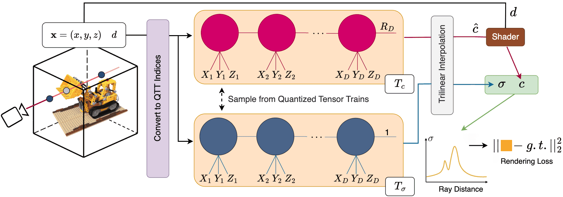
Figure 4: Novel view synthesis with PuTT. This illustration shows the process using two QTTs, $T_{\sigma}$ and $T_{c}$, for computing volume density ($\sigma$) and view-dependent color ($c$) through differential ray marching. For each 3D location $x=(x,y,z)$ and viewing direction $d$, $x$ is converted to QTT indices. These indices query the density voxel grid $T_{\sigma}$ and the color voxel grid $T_{c}$. The process uses trilinear interpolation to obtain continuous $\sigma$ values and appearance feature vectors $\hat{c}$. These vectors are processed through a shading module to generate raw color values $c$, which, along with $\sigma$, are used in differential volumetric rendering. The rendering loss is computed by comparing the generated color values against ground truth (g.t.) values.

5 Results

PuTT
PSNR 26.3, SSIM 0.72

TT No Upsampling
PSNR 25.7, SSIM 0.70

Tucker Upsampling
PSNR 21.8, SSIM 0.54

CP Upsampling
PSNR 21.6, SSIM 0.54

Figure 5: Qualitative comparison to baselines on 16k images.

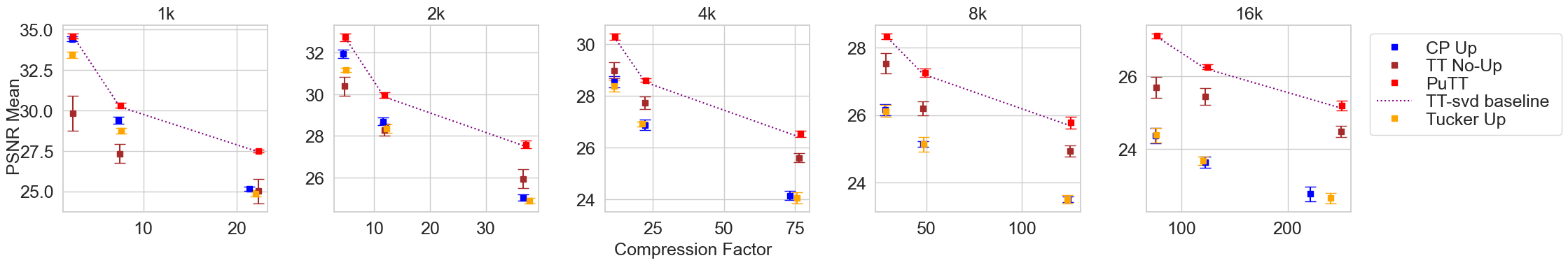
Figure 6: PSNR (y-axis) vs compression ratio (x-axis) for 2D fitting. “up = upsampling”.

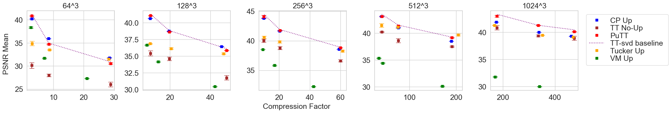
Figure 7: (a) PSNR (y-axis) in comparison to compression ratio (x-axis) for 3D fitting.

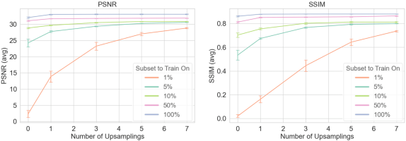
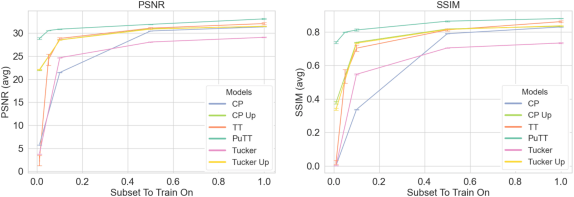
(a)	(b)

Figure 8: PSNR and SSIM vs number of upsampling steps for five different percentages of training data available (a) or vs different amounts of available training data available for three different models with or without upsampling (b). ”Up” refers to upsampling.

	Input	PuTT (Ours)	CP	Tucker	TT w/o up.	CP w/o up.	Tucker w/o up.
0.1 Noise
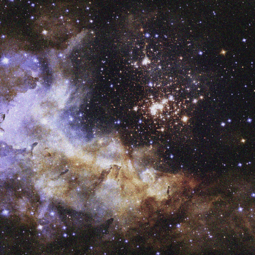
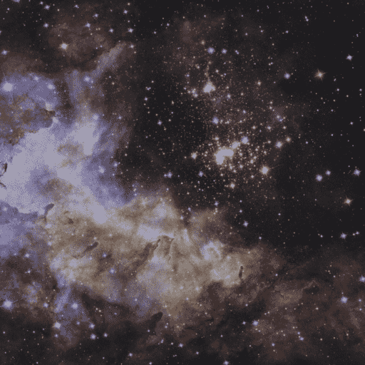
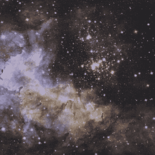
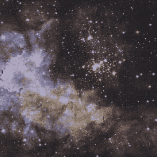
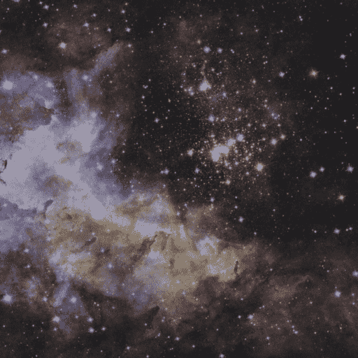
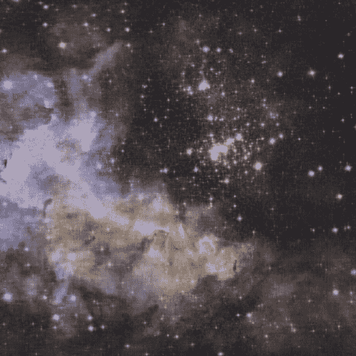
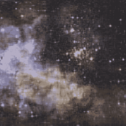
0.5 Noise
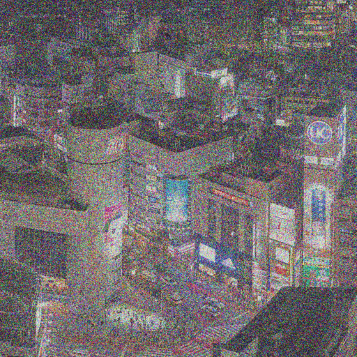
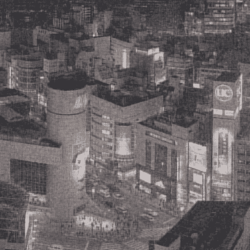
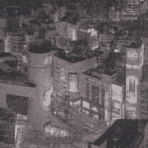
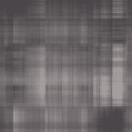
1.0 Noise

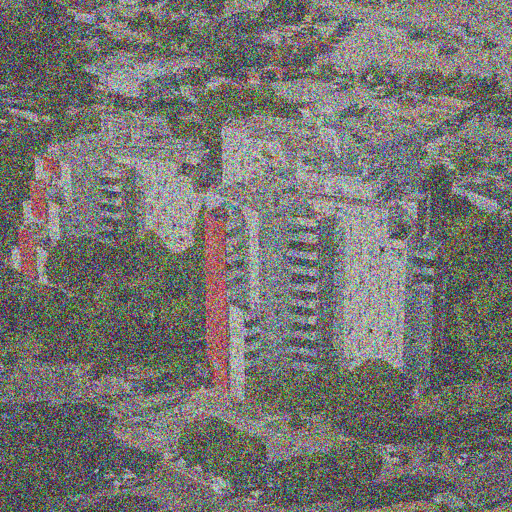
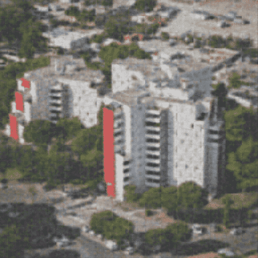
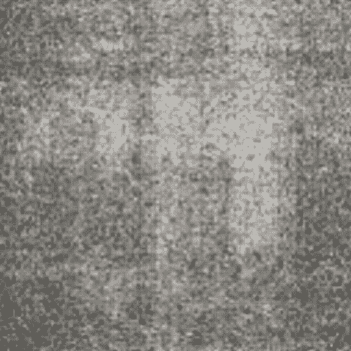
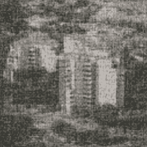
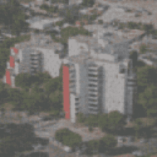
Figure 9: Visual comparison of training with noise levels $0.1$ (Top), $0.5$ (Middle),, and $1.0$ (Bottom). “W/o up = without upsampling”.

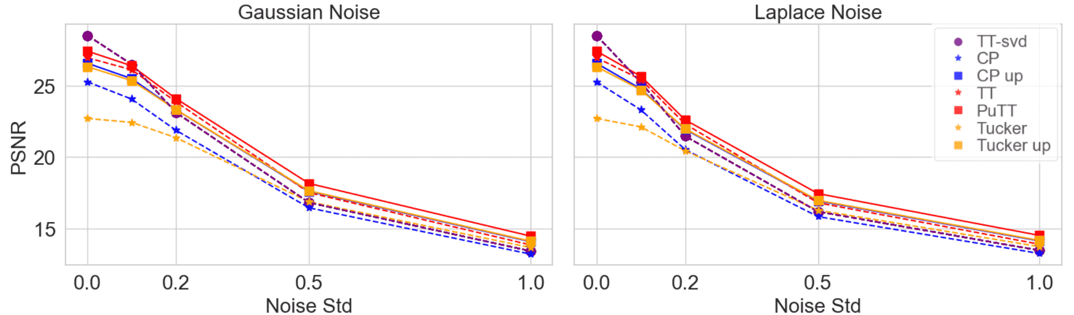
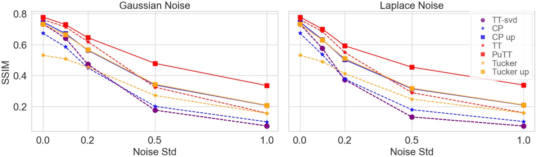
(a)	(b)

Figure 10: PSNR (a) and SSIM (b) when varying the amount of Gaussian or Laplacian noise for PuTT and baselines. “up = upsampling”.

We demonstrate the applicability of PuTT along three axes: (1). Compression, showing that PuTT can be optimized to achieve the expressive power and compactness of tensor trains, (2). Learning from missing data, showing that PuTT can learn to interpolate missing data effectively, (3). Denoising, showing that PuTT can better recover the original signal given noisy inputs. We evaluate these axes with respect to the applications of 2D fitting, 3D fitting, and novel view synthesis. Lastly, we conduct an ablation study to underscore the impact of individual components. In the appendix and supplementary webpage, we provide additional results accompanying existing figures and discuss the limitations.

Baseline Methods   We compare our method to state-of-the-art tensor-based methods: CP, Tucker, and the VM decomposition (Chen et al., 2022) (see details in Sec. 3 and appendix). Furthermore, we include a comparison with TT-SVD (Oseledets, 2011) (adapted to QTT, see appendix for details). TT-SVD is a deterministic approach, that starts from the full uncompressed tensor and compresses the tensor into tensor train form with a single pass over the input. TT-SVD and can only be applied when the direct signal (e.g., 2D image or 3D voxel grid) is provided, as it is applied analytically. It does not apply when optimization is required, such as in learning from missing data, or novel view synthesis, and does not perform well on noisy data. When referring to a baseline using upsampling, we train in a similar coarse-to-fine approach where the tensor factors are linearly interpolated to a finer grid using the approach developed by TensoRF (Chen et al., 2022). The term “TT” in our comparisons refers to training a QTT without adopting a coarse-to-fine learning approach.

Datasets   For 2D, we utilize two high-resolution images: “Girl With a Pearl Earring” (Vermeer, 1665) photograph, and “Tokyo gigapixel” (Dobson, 2018), which are center-cropped to a 16k resolution. We also include three 4k images: “Marseille” (Studio, 2023), “Pluto” (NASA/Johns Hopkins University, 2023), and “Westerlund” (NASA and ESA, 2023) for noise and missing data experiments. For 3D, we utilize the “Flower” data (of Zurich, 2023), and John Hopkins Turbulence dataset (Li et al., 2008), which consists of a set of 3D voxel grids at $1024^{3}$ resolution, providing a diverse range of high-resolution structures by downsampling to different resolutions. For novel view synthesis, we employ the Blender (Mildenhall et al., 2020) and NSVF (Liu et al., 2020a) datasets, comprising eight synthetic 3D scenes at $800\times 800$ resolution, alongside the TanksTemples (Knapitsch et al., 2017) dataset ($1920\times 1080$).

5.1 Compression

2D Compression  Fig. 5 provides a visual comparison to baselines while Fig. 6 provides a numerical one, showcasing PSNR results as a function of the compression ratio, defined as the ratio of uncompressed parameters to compressed parameters (Appendix shows corresponding SSIM results). Theoretically, QTTs have a logarithmic dependency on the image side length, while CP and Tucker have linear dependence. However, the tensor rank governs expressivity, and the tensor ranks of CP, Tucker, and QTT are not directly comparable; i.e. a QTT with max rank $50$ might be far more expressive than a CP with rank $50$. However, we clearly see the improved efficiency of QTT across different resolutions, which becomes more pronounced as the resolution increases across all compression ratios. At 16k resolution, PuTT significantly outperforms baselines, showing an advantage of over $2.5$ in PSNR and $0.1$ in SSIM. PuTT performs better than the analytical TT-SVD in all 2D scenarios in terms of PSNR. For SSIM, PuTT consistently outperforms TT-SVD up to 8k resolution, with a minimum improvement of $0.05$ SSIM across all compression ratios. At 16k resolution, TT-SVD exhibits better SSIM, indicating the challenges in capturing structural image properties as the resolution and the ratio between batch size and image size increase. The CP, Tucker, and QTT ranks were adapted to match the target compression ratios shown in the figure.

			Synthetic-NeRF		NSVF		TanksTemples
Method	Steps	Size(MB)$\downarrow$	PSNR$\uparrow$	SSIM$\uparrow$	PSNR$\uparrow$	SSIM$\uparrow$	PSNR$\uparrow$	SSIM$\uparrow$
PlenOctrees* (Yu et al., 2021b)-L	200k	1976.3	31.71	0.958	-	-	27.99	0.917
Plenoxels* (Yu et al., 2021a)-L	128k	778.1	31.71	0.958	-	-	27.43	0.906
DVGO* (Sun et al., 2022)-L	30k	612.1	31.95	0.957	35.08	0.975	28.41	0.911
K-planes* (Fridovich-Keil et al., 2023)-L	30k	122.1	32.36	0.962	-	-	-	-
Instant-NGP* (Müller et al., 2022)-L	35k	45.5	33.18	0.963	-	-	-
TensoRF (Chen et al., 2022) VM-192*-L	30k	71.8	33.14	0.963	36.52	0.982	28.56	0.920
Our PuTT-600-L	80k	60.3	32.79	0.958	36.57	0.982	28.37	0.917
NeRF* (Mildenhall et al., 2020)-S	300k	5.0	31.01	0.947	30.81	0.952	25.78	0.864
TT-NF * (Obukhov et al., 2022)-S	80k	7.9	31.09	0.945	-	-	-	-
TensoRF CP-384*-S	30k	3.9	31.56	0.949	34.48	0.971	27.59	0.897
TensoRF VM-30 (no shrinking)-S	80k	6.9	31.10	0.948	34.57	0.974	27.67	0.898
Our PuTT-200-S	80k	6.7	31.66	0.956	35.58	0.976	27.99	0.901
TensoRF VM-48 (no shrinking)-M	80k	12.0	31.62	0.952	35.44	0.976	28.03	0.901
Our PuTT-280-M	80k	12.0	31.95	0.957	36.04	0.977	28.15	0.905

Table 1: Comparison to baselines for the task of novel view synthesis for the Synthetic-NeRF (Mildenhall et al., 2020), NSVF (Liu et al., 2020a), and TanksTemples (Knapitsch et al., 2017) datasets. Scores of the baseline methods with a $*$ are taken directly from corresponding papers whenever possible. L, M and S indicate a Large ($>60$ MB), Medium ($12$ MB) or small ($<8$ MB) model size. We compare our method on Medium and Small-sized models but also include Large-sized models for reference.

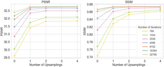
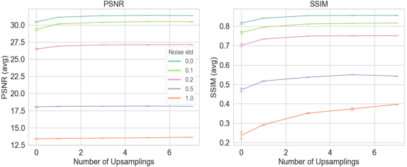
(a)	(b)

Figure 11: PSNR and SSIM for PuTT, under varying iteration counts (a) and varying levels of Gaussian noise ($\sigma$) (b).

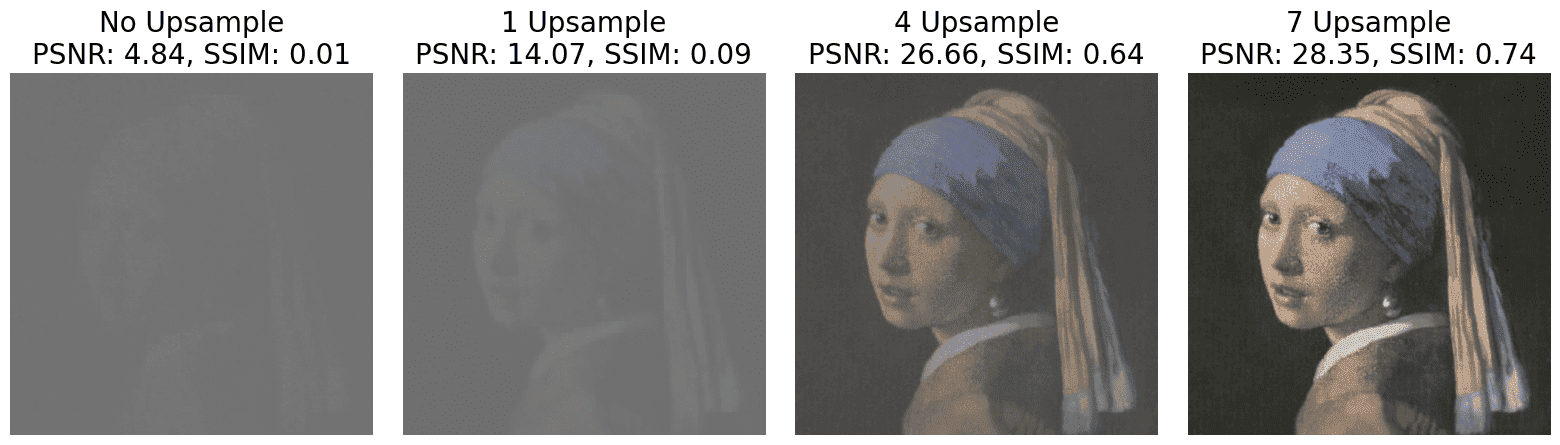
Figure 12: Varying the number of upsampling steps when training $99\%$ missing data. The first image displays the training data, followed by PuTT results with $0,1,4$, and $7$ upsampling steps.

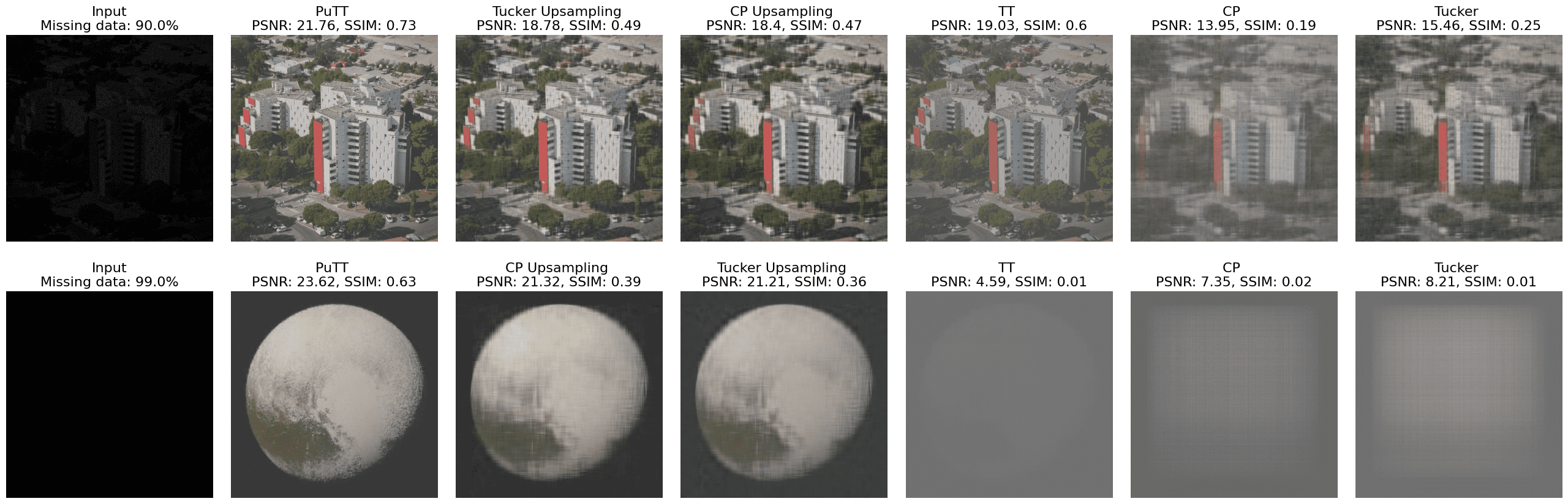
Figure 13: Visual comparison of PuTT to baselines when training with $90\%$ (Top) and $99\%$ (Bottom) missing data.

	Chair		Ficus		All Scenes
	TensoRF	PuTT	TensoRF	PuTT	TensoRF	PuTT
Near	35.59	37.12	32.53	33.95	31.93	32.93
Far	31.74	32.71	30.16	31.06	28.97	29.41
All	32.22	33.50	30.71	31.69	30.43	31.66

Table 2: Novel view synthesis comparison to TensoRF (PSNR) on the Chair, Ficus, and all scenes (Blender dataset (Mildenhall et al., 2020)). We test on views near training (Near), far from training (Far), and all test views (All). See the appendix for all details.

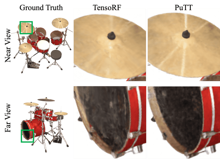
Figure 14: Visual comparison of a single NeRF for “drums”.

3D Compression  In 3D, we observe similar trends, as shown in the Fig. 7 (PSNR) and appendix (SSIM). However, the dynamics differ notably among the PuTT, CP, and Tucker at various resolutions. Up to $256^{3}$, CP and Tucker perform closely to PuTT. Yet, for $1024^{3}$, PuTT significantly outshines the other methods, leading to more than $1$ PSNR improvement and nearly $0.005$ improvement in SSIM. VM’s performance is less substantial due to its quadratic dependency on the side length, unlike the linear dependency of CP and Tucker and the logarithmic dependency of QTT. VM shows relatively poor performance. This is attributable to the high compression setting of our experiment, coupled with VM’s quadratic dependency on side length. PuTT is comparable to deterministic TT-SVD, but achieving high SSIM is exacerbated at larger resolutions, underscoring the increased difficulty in maintaining image quality at higher compression settings. One might speculate that the crossover in efficiency, where it pays off to use the QTT representation, occurs around sidelength $L=512$.

Novel View Synthesis  As seen in Tab. 1, PuTT outperforms TensoRF when using high compressions (7MB and 12MB) for Blender, NSVF, and TanksTemples datasets and has comparable performance on the large model size. We evaluate models in three sizes: Large ($>$60 MB), Medium (12 MB), and Small ($<$8 MB). Our 12MB PuTT model, despite having six times fewer parameters, matches the performance of the Large baselines on the NSVF and TanksTemples datasets. Moreover, our 7MB PuTT model outperforms Small baselines by over one PSNR on the NSVF dataset. For a detailed overview of the implementation, please consult the appendix. In Tab. 2, for the 7MB size, we consider a more detailed comparison, distinguishing between near and far views at test time. Our improvement is more pronounced at nearby views, indicating our ability to capture fine details better than TensoRF. Fig. 14 demonstrates visually our ability to better capture fine-grained details. In Appendix G we provide per-scene results.

5.2 Learning from Incomplete Data

We evaluate the capability of PuTT to learn 2D or 3D representations by training only on a subset of the available data, thus assessing its generalizability. We randomly select a percentage $p\%$ of the full input data $I_{D}$. This yields a subset of indices, $\mathcal{I}_{D,p}$, which we use exclusively for training. We evaluate the performance of the full input data, including untrained indices. To train with a down-sampled target at lower resolutions, we create a modified target image $I_{D-l,p}$. We build $I_{D-1,p}$ from $I_{D,p}$, we use a custom masked average pooling method, averaging only the non-zero values in each window, sized according to the downsampling factor. The resulting downsampled image, $I_{D-l,p}$, thus contains aggregated information within each patch of size $2^{l}\times 2^{l}$ of $I_{D,p}$. Any non-zero value in $I_{D-l,p}$ represents aggregated data from the original data within the corresponding patch. This forms a new set of indices $\mathcal{I}_{l,p}$, from which we sample during training on the downsampled input $I_{D-l,p}$. Fig. 8(a) considers the effect of varying the number of upsampling steps, when training with different training data percentages (see visual examples in Fig. 12). It illustrates the significance of upsampling when learning from limited data samples, highlighting its growing importance as training data size decreases. Without upsampling, training on just $1\%$ of the input, PuTT gets a PSNR of $1.87$ and SSIM of $0.0018$. However, applying seven upsampling steps enhances the results to a PSNR of $28.73$ and SSIM of $0.7349$. Similar improvements are observed with $10\%$ training data. Fig. 8(b) shows PuTT consistently surpasses CP and Tucker, especially at lower resolutions. Fig. 13 gives a visual example when $90\%$ and $99\%$ of the data is missing for PuTT and baselines, showing a better recovery of the input image.

5.3 Noise Removal

We aim to learn a tensor representation of a target, denoted as $\mathcal{X}_{I}$, using samples from its noisy counterpart, $\hat{\mathcal{X}}_{I}$, obtained by adding noise $Z$. In our experiments, $Z$ is sampled from either a Normal or Laplacian distribution (see details in appendix). At training, we minimize $||\hat{\mathcal{X}}_{I}-R_{T}||^{2}_{2}$. At inference, we compare the learned $R_{T}$ with the original clean target $\mathcal{X}_{I}$. As shown in Fig. 10(a), PuTT consistently achieves higher PSNR than other tensor network methods across various levels of noise sigma. Notably, the application of upsampling not only avoids overfitting to noisy samples but also consistently outperforms the non-upsampling approach. Fig. 10(b) underscores the clear benefits of employing upsampling strategies. This is particularly evident in PuTT, where upsampling yields an SSIM score improvement of more than $0.1$ for noise levels exceeding $0.2\sigma$.

Fig. 9 shows recovered images, both with and without upsampling at Gaussian noise levels of $\sigma=0.05,0.5,1.0$. These examples highlight the efficacy of upsampling in mitigating noise, demonstrating visibly superior results compared to models not utilizing upsampling. Moreover, PuTT showcases enhanced details and a more effective noise-filtering capability because of its hierarchical structure.

5.4 Ablation Study

Fig. 11(a) illustrates the impact of varying the number of upsamplings and the number of iterations on efficiency. The results highlight the efficiency of our method: using just $1024$ iterations with four upsampling steps, we achieve comparable PSNR and SSIM to training without upsampling for $16$k iterations. Beyond $4$k iterations, there is no significant improvement in quality. Without upsampling this plateau is not reached even after $32$k iterations. More upsampling steps notably enhance SSIM because SSIM is sensitive to global features like overall mean, standard deviation, and luminance. Training on downsampled inputs using tensor trains, which involves gradient updates based on batches covering larger portions of the input, seems to facilitate learning these global characteristics more effectively.

Fig. 11(b) presents an ablation study on the ”Girl with a Pearl Earring” image at 4k resolution and rank $200$, with a fixed iteration count of $8192$. We examine the impact of varying the number of upsampling steps on the model’s performance, for varying degrees of Gaussian noise applied on the input. The LHS of Fig. 11(b) illustrates the influence of the first upsampling step on PSNR, showing a notable improvement. Subsequent upsampling steps result in incremental gains. The SSIM plot, on the RHS, reveals a more pronounced improvement with each upsampling step, indicating the effectiveness of upsampling in enhancing the model’s ability to learn global features.

These findings are supported by additional experiments and analyses in the appendix. Sec. C highlights the statistical robustness of our experiments, showing minimal variation with upsampling compared to without. Sec. E examines the influence of initialization, demonstrating PuTT’s consistent performance across different initialization values. Without upsampling, QTT training is sensitive to initialization standard deviation, with PSNR fluctuating between $34.958$ (std $0.05$) and $12.320$ (std $0.5$) for a $512\times 512$ RGB image. In contrast, PuTT’s PSNR remains stable between $36.100$ and $36.116$ for std values from $0.001$ to $0.5$. Sec. J shows how rank incrementation strategy inspired by SlimmeRF (Yuan & Zhao, 2023) can further improve performance.

6 Conclusion

We proposed a novel coarse-to-fine, Tensor-Train-based representation called ‘Prolongation Upsampling Tensor Train (PuTT)’ and an associated optimization strategy. This approach involves prolonging or “upsampling” a learned Tensor Train representation, creating a sequence of tensor trains that are incrementally refined in a coarse-to-fine manner. We demonstrated the applicability of our method along the axes of compression, learning from missing data, and denoising. We evaluated these axes with respect to the applications of 2D fitting, 3D fitting, and novel view synthesis and demonstrated state-of-the-art performance compared to other tensor-based methods, especially in high-compression settings. Our learning scheme leverages the improved compression ability and multi-resolution nature of the Quantized Tensor Train (QTT) for improved denoising and image completion capabilities. In future work, we hope to apply PuTT to large-scale Neural Radiance Fields (NeRFs) and dynamic neural fields, utilizing the logarithmic dimensionality advantages of QTTs to represent large and finely detailed scenes.

Acknowledgements  Sebastian Loeschcke is supported by the Danish Data Science Academy, which is funded by the Novo Nordisk Foundation (NNF21SA0069429) and VILLUM FONDEN (40516). Serge Belongie and Dan Wang are supported by the Pioneer Centre for AI, DNRF grant number P1. MJK acknowledges support from the Carlsberg Foundation and the Novo Nordisk Foundation.

Impact Statement  This paper contributes to the Machine Learning field by enhancing visual representation learning using tensor train optimization. Given the current stage of our research, we identify no specific ethical issues warranting exploration. Nonetheless, we acknowledge the dynamic nature of technological impacts and pledge to continually assess the ethical implications as our research advances.

This appendix material complements the main paper by providing detailed explanations and extended analyses.

Sec. A discusses the supplementary webpage. In Sec. B, we discuss the limitations of our approach and its constraints and boundaries. In Sec. C, we discuss the statistical robustness of our experiments. In Sec. D, we give detailed descriptions of various tensor network methods, their complexities, and specific adaptations for our study. Sec. E, we discuss the influence of initialization on model performance. In Sec. F, we provide insights into our experimental framework, including batch sizes, learning rate strategies, and handling of noise and incomplete data. In Sec. G, we provide additional novel view synthesis results. In Sec. H, we explain the compatibility of TensoRF’s ”shrinkage” with QTT. In Sec. I, we explore the inpainting capabilities with PuTT. In Sec. J, we explore rank incrementation with SlimmeRF (Yuan & Zhao, 2023).

Appendix A Supplementary Webpage

Additional supplementary materials and the associated code can be accessed at https://sebulo.github.io/PuTT_website/.

Appendix B Limitations

In our compression results in Sec. 5.1 of the main text, we observe certain constraints associated with our PuTT method. While learning QTT representations using PuTT show a marked advantage in scenarios requiring high compression, as evident in our results for 2D and 3D data (Figures 6, 7) and in Novel View Synthesis (Tab. 1 of the main text), their effectiveness tends to converge with other methods like CP, Tucker, and VM in less compressed settings with smaller tensor sizes. For example, in the case of 1k resolution images (referenced in Sec. 5.1, Fig. 6 of the main text), we noted that the performance benefits of using QTTs were less pronounced. This suggests that while QTTs are highly effective in handling large-scale, high-compression tasks, their advantages are less significant in simpler scenarios with lower compression.

Appendix C Sensitivity and Statistical Analysis

In our experimental framework, we tested each configuration using three distinct seeds to ensure the reliability and consistency of our results. We use error bars representing $\pm 1$ standard deviation from the mean in all plots. In the context of our 2D and 3D experiments, it’s noteworthy that the error bars are often so minimal (see Sec. 5.1 of the main text, Fig. 6) that they might be challenging to discern in the plots. This observation points to a low degree of variation, suggesting a high level of reproducibility in our results. Such consistency is particularly evident in experiments involving upsampling, where a consistent trend towards similar endpoints in training was observed. This pattern can be attributed to the progressive nature of our approach, which systematically builds the representation on increasingly finer grids. Furthermore, when comparing the performance of our PuTT method with other established methods like Tucker, CP, and VM, we observed less variation in PuTT’s performance across different experimental setups. This reduced variability, especially visible in the compression plots, indicates that PuTT not only ensures a more stable and predictable performance but also underscores its effectiveness in different experimental conditions and settings.

C.1 Enhancing Training Stability through Upsampling

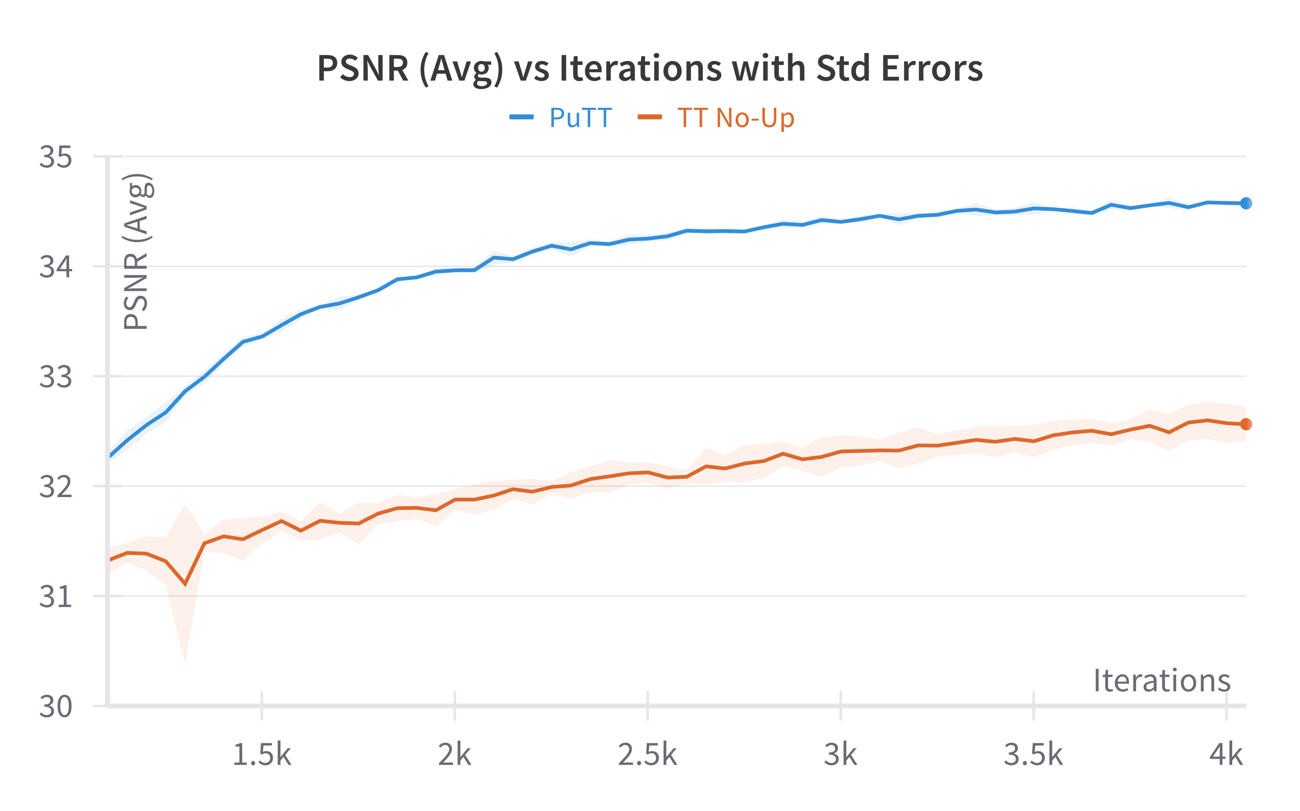
(a) Girl 4K

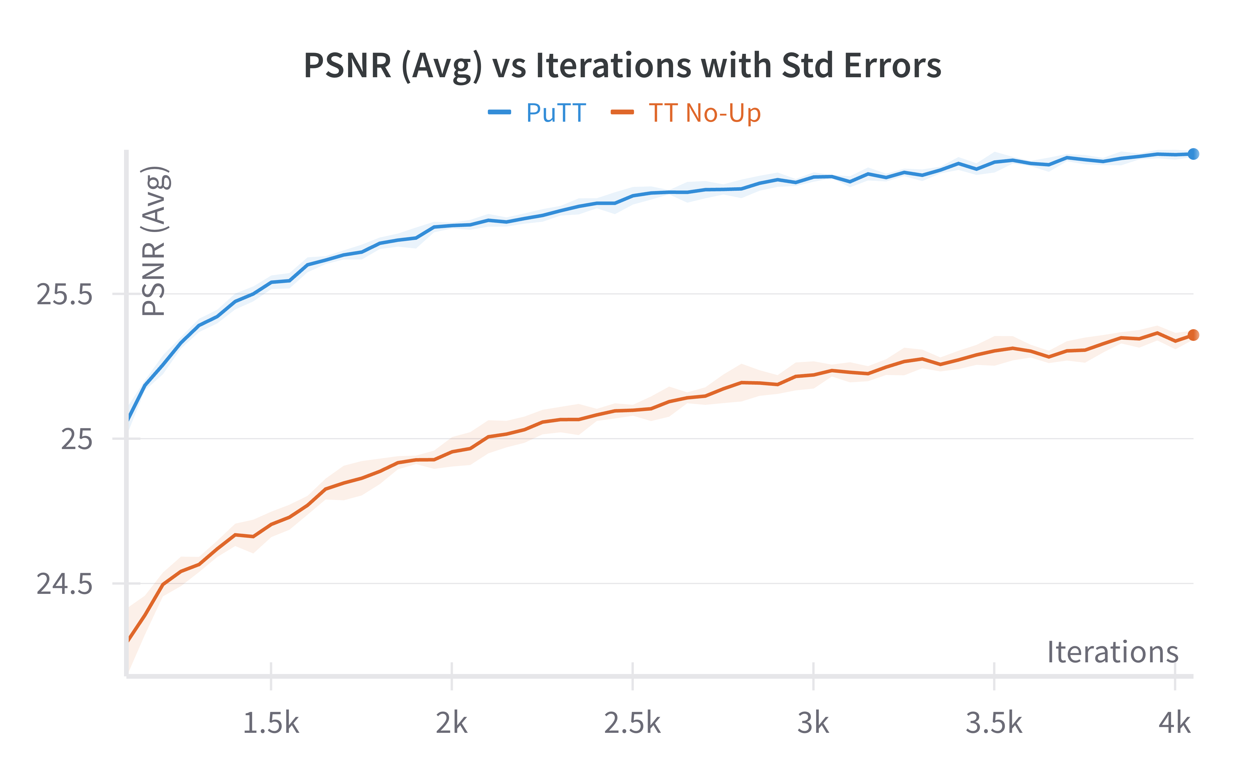
(b) Tokyo 4K

Figure 15: The two figures present plots corresponding to the ”Girl with Pearl Earring” (15(a)) and ”Tokyo” 4K images (15(b)), showcasing the performance of our PuTT method with upsampling versus a baseline QTT model without upsampling. For both images, we plot the average PSNR over $4000$ iterations, averaged across three seeds. The shaded regions around each curve represent the variability within $\pm 1$ standard deviation from the mean PSNR, serving as an indicator of training stability. In both plots, it is evident that the upsampling model exhibits lower fluctuation in standard deviation and achieves higher PSNR levels by the end of the training period. This highlights the improved stability and effectiveness of our upsampling approach in 2D compression tasks.

Figure 15 shows an experiment further illustrating the stabilizing effect of our upsampling strategy within the context of 2D compression tasks. The experiment analyses the ”Girl with Pearl Earring” and ”Tokyo” images, both at 4K resolution, to draw comparisons between our upsampling approach and a baseline QTT model with no upsampling. The findings, visualized in our plot, reveal the average PSNR against the number of iterations, with the shaded area depicting the variance within $\pm 1$ standard deviation across three separate runs. This comparison underscores the enhanced stability of training with our upsampling method, evidenced by reduced performance fluctuations and consistently higher PSNR levels compared to models without upsampling.

Appendix D Tensor Networks

We describe the three main families of tensor decompositions that are considered in this work: CP/VM, and Tucker. Tensor Trains and the specific QTT format are defined in the main article. We provide additional information on MPOs and the general complexity of manipulating tensor networks.

The canonical polyadic (CP) decompositions (Carroll & Chang, 1970; Harshman, 1970)

factorizes a tensor $\mathcal{T}\in\mathbb{R}^{n_{1}\times n_{2}\times\cdots n_{d}}$ into a sum of rank-$1$ components:

$$\mathcal{T}=\sum^{R}_{r=1}v_{r}^{1}\otimes v_{r}^{2}\otimes\cdots\otimes v_{r}^{d}$$ (2)

where $v^{1}_{r},v_{r}^{2},\cdots,v_{r}^{d}$ are rank-$1$ vectors in $\mathbb{R}^{n_{1}},\cdots,\mathbb{R}^{n_{d}}$. Each tensor element is then a sum of scalar products:

$$\mathcal{T}_{j_{1}\cdots j_{d}}=\sum^{R}_{r=1}\sum_{k=1}^{d}v_{r,j_{k}}^{k},$$ (3)

where $j_{k}=1,...,n_{k}$ for each $k=1,...,d$. We will mostly consider $d=2,3$ in this work, as we care about visual data.

The Vector Matrix (VM) decomposition (Chen et al., 2022)

is a specific 3D tensor decomposition, introduced to remedy a ”too high” compactness of the CP decomposition. Instead of purely using vector factors, the VM decomposition factorizes a tensor into vectors and matrices. For $\mathcal{T}\in\mathbb{R}^{n_{1}\times n_{2}\times n_{3}}$,

$$\mathcal{T}=\sum^{R_{1}}_{r=1}v_{r}^{1}\otimes M_{r}^{2,3}+\sum^{R_{2}}_{r}v_{r}^{2}\otimes M_{r}^{1,3}+\sum_{r=1}^{R_{3}}v_{r}^{3}\otimes M_{r}^{1,2}$$ (4)

where the superscript on the vectors $v$ and matrices $M$ indicate the space on which they act. The VM decomposition can be understood as a half-way between the dense (bare) representation of $\mathcal{T}$ and the CP decomposition. As such, VM has reduced compression as compared with CP. The overall rank of the VM decomposition is equal to the total number of components $(R_{1}+R_{2}+R_{3})$.

The Tucker decomposition (Tucker, 1966)

provides only a partial compression of a tensor. Given a tensor $\mathcal{T}\in\mathbb{R}^{n_{1}\times n_{2}\times\cdots n_{d}}$, we define a reduced tensor $\mathcal{K}\in\mathbb{R}^{m_{1}\times m_{2}\times\cdots m_{d}}$ and matrices $U^{k}\in\mathbb{R}^{m_{k}\times n_{k}}$, such that

$$\mathcal{T}_{j_{1},...,j_{d}}=\sum_{i_{1}=1}^{m_{1}}\cdots\sum_{i_{d}}^{m_{d}}\mathcal{K}_{i_{1},...,i_{d}}U^{1}_{i_{1},j_{1}}\cdots U^{d}_{i_{d},j_{d}}.$$ (5)

The Tucker decomposition is mostly useful in settings where $d$ is small, and $n_{k}$ are large.

Matrix Product Operators

A matrix product operator (MPO) is a tensor network that describes a factorization of a tensor with $d$ input and $d$ output indices into a linear network of smaller tensors (Hubig et al., 2017; McCulloch, 2008). Each core (except for the first and last) has two physical indices and two virtual indices.

The difference between TTs and MPOs is the nature of the objects they are meant to represent. A TT can be seen as a parameterization of a large vector in a high-dimensional space, providing a compressed yet expressive representation of such vectors. The ”operator” part of the term ”Matrix Product Operator” refers to the mathematical operation of a matrix acting on a vector (Stoudenmire, 2021), i.e., the MPO operates on a TT. This essentially allows one to efficiently represent and work with large operators in high-dimensional spaces, working directly in the compressed TT representation.

Using the same index notation as for TTs, an MPO is a tensor network of the form:

$$\mathcal{M}_{i_{1}...i_{d}}^{j_{1},...,j_{d}}=A^{i_{1},j_{1}}A^{i_{2},j_{2}}...A^{i_{d},j_{d}},$$ (6)

where $A^{i_{k},j_{k}}$ are $R_{k}\times R_{k+1}$ matrices for each pair $i_{k},j_{k}$. MPOs have important applications in representing large, sparse matrices in a form that is convenient for TT algorithms (White, 1992a; Holtz et al., 2012; Lubasch et al., 2018). They play a central role in TT algorithms in Physics, yet have been under-exploited in the data science setting. Here we show how to leverage MPOs in the visual data setting in connection with multi-resolution analysis.

Complexity of the CP, VM, Tucker, and TT decompositions

Given a tensor with $d$ indices of maximal dimension $n$, CP decomposition stores $dR_{CP}$ rank-$1$ tensors of size $n$, resulting in a space complexity of $O(dnR_{CP})$. Here, $R_{CP}$ is the CP rank. In 3D, the VM decomposition stores $R_{VM}$ times a size $n$ vector and a $n\times n$ matrix, resulting in a space complexity $O(R_{VM}(n+n^{2}))$. The Tucker decomposition stores a tensor $\mathcal{K}$ with maximal index range $m$ and $d$ matrices of size $n\times m$ resulting in a space complexity $O(dm^{d+1}n)$. Finally, the tensor train stores $nd$ matrices of size $R_{TT}^{2}$, resulting in a space complexity $O(ndR_{TT}^{2})$.In practice, the complexity is lower, as one can further exploit the tensor network structures to reduce the individual ranks in the network.

If $d$ is large - typically $d>3$ - then we expect the memory cost to scale as Tucker, CP $\gg$ TT. While the separation between Tucker and TT is obvious, since Tucker scales exponentially in $d$, the separation between CP and TT is contained in the rank dependence. For fixed accuracy, we expect TT to require a constant rank $R_{TT}$, independent of $d$. While the CP rank $R_{CP}$ will grow up to exponentially in $d$ (Kolda & Bader, 2009).

However, with visual data, we have $d\leq 4$, hence the relationships are more subtle and depend crucially on the representational power of each decomposition; i.e. what ranks are necessary to represent visual data up to a given precision, and whether these representations can be learned in an efficient and reliable manner. In the QTT representation, the complexity is $O(2^{d}\log(n)R^{2})$.

In summary, one should expect that for $d=2,3,4$ and large $n$ (i.e. high resolution), the QTT format should outperform CP, VM, and Tucker, with the gap growing up to exponentially as $d$ and $n$ grow.

Computational Complexity of Prolongation:

For a tensor $T$ of dimensions $D^{N}$, where $N=2$ typically represents the dimensions of an image (height and width), the upper bound for the computational complexity involved in multiplying a Matrix Product Operator (MPO) with a Quantized Tensor Train (QTT) is denoted by $O(\log(D)\cdot\max(R,S)^{3}\cdot N^{D})$. In this expression, $(\log(D))$ denotes the number of cores in the QTT, which corresponds to the level of quantization. $(R)$ and $(S)$ are the maximum ranks within the QTT and MPO, respectively. This operation is efficiently executed and does not significantly influence the overall runtime.

Implementation

When learning tensor networks such as Tucker, CP, TT, QTT, and VM, especially in challenging scenarios with noisy, incomplete data or in applications like NeRF where the full scene tensor is not accessible, it becomes essential to adopt a sample-based training approach. Unlike traditional analytic techniques such as Higher-Order Singular Value Decomposition (HOSVD) (Tucker, 1966) for Tucker decomposition, or Singular Value Decomposition (SVD) and QR decompositions for TT (Oseledets, 2011) and QTT (Khoromskij, 2011), our methodology does not rely on these direct decomposition methods. Instead, we commence with an initial skeleton tensor that mirrors the structure required by the chosen decomposition scheme. This skeleton serves as a starting point for an iterative optimization process, where the tensor values are refined using stochastic gradient descent. This approach allows for a flexible and efficient adaptation of the tensor factorization methods to the intricacies and limitations of the data and application context, such as those encountered in NeRF scenarios.

D.1 Multiresolution Format of Quantized Tensor Train

The multiresolution format, as explained in Sec.3, is illustrated in Fig.16.

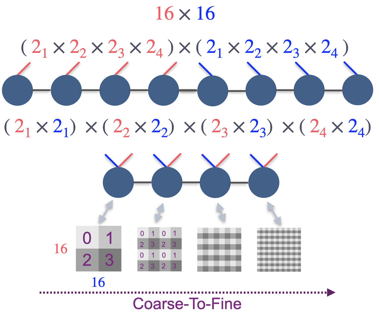
Figure 16: This figure illustrates the transformation of a 16x16 matrix into QTT format, showcasing a transition from a standard grid representation to a mixed factor order. Initially presented as a simple $16_{x}$ by $16_{y}$ matrix, it is restructured into factors of two: $\left(2_{1x}\times\right.$ $\left.2_{2x}\times 2_{3x}\times 2_{4x}\right)$ combined with $\left(2_{1y}\times 2_{2y}\times 2_{3y}\times 2_{4y}\right)$. Subsequently, the factors are permuted into a mixed factor order $\left(2_{1x}\times 2_{1y}\right)\times$ $\left(2_{2x}\times 2_{2y}\right)\times\left(2_{3x}\times 2_{3y}\right)\times\left(2_{4x}\times 2_{4y}\right)$. This results in a multiresolution format where the initial core’s indices correspond to indexing into four quadrants of the input matrix. Specifically, index 0 in the first core is associated with the top-left quadrant of the grid. Subsequent cores progressively examine increasingly detailed segments of the matrix. This hierarchical breakdown allows the QTT to capture and represent data at various levels of granularity, starting from broad, overarching structures down to more intricate details within the grid, which is reminiscent of a wavelet.

D.2 The prolongation operators

We employ a Matrix Product Operator (MPO) known as a prolongation operator $\mathcal{P}$, suggested by Lubach et al. (Lubasch et al., 2018), to upsample coarse solutions in the Quantized Tensor Train (QTT) format.

Consider a one-dimensional vector $v_{d}\in\mathbb{R}^{2^{d}}$ representing data like a continuous function. To achieve a finer representation $v_{d+1}\in\mathbb{R}^{2^{d+1}}$, we linearly interpolate between adjacent points in $v_{d}$ using the matrix $P_{2^{d}\rightarrow 2^{d+1}}$. This matrix resembles the Haar transform matrix. For instance for $d=2$, we can express $P_{2^{d}\rightarrow 2^{d+1}}$ as:

$$P_{4\rightarrow 8}=\left(\begin{matrix}.5&0&0&0\\ 1&0&0&0\\ .5&.5&0&0\\ 0&1&0&0\\ 0&.5&.5&0\\ 0&0&1&0\\ 0&0&.5&.5\\ 0&0&0&1\\ \end{matrix}\right),$$ (7)

This matrix is closely related to the Haar transform matrix. The matrix $P_{2^{d}\rightarrow 2^{d+1}}$ can be written as an MPO $\mathcal{P}$ with bond dimension two as

$$\mathcal{P}_{j_{1},...,j_{n}}^{i_{1},...,i_{n},i_{n+1}}=P[1]^{j_{1},i_{1}}\cdots P[d]^{j_{d},i_{d}}P[d+1]^{i_{n+1}}.$$ (8)

The middle $d-1$ tensors in the MPO, $P[k]^{j_{k},i_{k}}_{\alpha_{k},\alpha_{k+1}}$ have two physical indices $j_{k},i_{k}$ and two virtual indices $\alpha_{k},\alpha_{k+1}$. Each index $i_{k},j_{k},\alpha_{k}\in[0,1]$. The first tensor $P[1]^{j_{1},i_{1}}_{\alpha_{1}}$ has one virtual index $\alpha_{1}$ and two physical indices $j_{1},i_{1}$, while the last tensor $P[d+1]^{i_{d+1}}_{\alpha_{d}}$ has one virtual index $\alpha_{d}$ and one physical index $i_{d+1}$. The entries are given explicitly as:

$$P[1]_{0}^{0,0} = P[1]_{0}^{1,1}=P[1]_{1}^{1,0}=1$$

$$P[k]_{0,0}^{0,0} = P[k]_{1,0}^{0,1}=P[k]_{0,1}^{1,1}=P[i]_{1,1}^{1,0}=1,$$

$$\text{for }1<k<d+1$$

$$P[d+1]_{0}^{0} = 1,\quad\text{and }P[d+1]_{0}^{1}=P[d+1]_{1}^{1}=\frac{1}{2},$$

with all other entries being zero (Lubasch et al., 2018).

The previously described prolongation operator $\mathcal{P}$ applies to tensor train representations of one-dimensional tensors in QTT format. In higher dimensions, the prolongation operator is simply the tensor product of the one-dimensional operators on each dimension: $\mathcal{P}\bigotimes\mathcal{P}$ for $2$-dimensions and $\mathcal{P}\bigotimes\mathcal{P}\bigotimes\mathcal{P}$ for $3$-dimensions.

D.3 Quantized Tensor Train Initialization

We initialize the TT-ranks between each core to follow a trapezoid structure like first introduced by Oseledets et al. (Oseledets, 2011). In a trapezoid structure, the TT-ranks may increase up to a certain point (creating the rising edge of the trapezoid), then stay constant, and then decrease (creating the falling edge of the trapezoid). The top (flat part) of the trapezoid corresponds to the maximum rank among all cores, which is what we call the TT-rank.

This structure can be beneficial because it allows representing a high-dimensional tensor in a compressed form which still maintains a good approximation of the original tensor (Oseledets, 2011).

To compute the TT-ranks in the context of the trapezoid structure, consider an array containing the $D$ physical indices of a TT $n=[n_{1},n_{2},\ldots,n_{D}]$. The TT-ranks are derived as follows:

1. Compute the cumulative product of the tensor shape from left to right and from right to left, denoted as ranks_left and ranks_right respectively:

   $$\texttt{ranks\_left}[i] =\prod_{j=1}^{i}n_{j},\quad\forall i=1,\ldots,D$$

   $$\texttt{ranks\_right}[i] =\prod_{j=i}^{D}n_{j},\quad\forall i=1,\ldots,D$$

2. Then, calculate the TT-ranks by taking the minimum of the ranks_left and ranks_right at each position:

   $$\texttt{ranks\_tt}[i] =\min(\texttt{ranks\_left}[i],\texttt{ranks\_right}[i]),$$

   $$\quad\forall i=1,\ldots,D$$

3. Finally, if a rank, max_rank, is specified, ensure that no index rank exceeds this value:

   $$\texttt{ranks\_tt}[i] =\min(\texttt{ranks\_tt}[i],\texttt{max\_rank}),$$

   $$\quad\forall i=1,\ldots,D$$

From this, it follows that if the payload dimension is greater than $1$, then we have to scale the dimensions of each core from the left to the right until we reach the rank top of the trapezoid structure of the TT.

$$\hat{\sigma}=\exp\left(\frac{1}{2D}\left(2\log\sigma-\Sigma_{i=1}^{D}\log R_{i}\right)\right)$$ (9)

D.4 TT-SVD Baseline

The Tensor Train - Singular Value Decomposition (TT-SVD) algorithm, as detailed by Oseledets et al. (Oseledets, 2011), offers a method for decomposing high-dimensional tensors into tensor trains. It sequentially reshapes and applies matrix SVD to each tensor mode, transforming a high-dimensional tensor into a series of interconnected lower-dimensional tensors, effectively forming a tensor train. For an in-depth understanding of TT-SVD, Oseledets et al.’s work provides comprehensive details.

As also pointed out in Sec. 10 of the main text, TT-SVD has limitations, particularly in its applicability only when the direct signal (e.g., a 2D image or 3D voxel grid) is provided for an analytical application. It falls short in scenarios requiring optimization, such as learning from incomplete data, novel view synthesis, or handling noisy data. Another limitation of TT-SVD is its infeasibility when the input tensor is too large for memory.

In our work, TT-SVD, implemented via the TNTorch framework (Usvyatsov et al., 2022), serves as a baseline to determine whether our Prolongation Upsampling Tensor Train (PuTT) method can escape local minima without specific hyperparameters. This benchmarking aids in assessing PuTT’s effectiveness in handling large-scale tensor data and its ability to navigate the challenges of optimization. In our implementation, we adapt TT-SVD for the QTT format. This adaptation involves initially reshaping the input tensor into $\log(N)$ factors of $2$, rearranging these factors to enforce Z-order correlation between spatial dimensions, and then applying TT-SVD. This process aligns with how we typically construct the specialized QTT structure.

D.5 Differences Between Vector Quantization and QTT

VQ compresses data by mapping input vectors to a set of discrete symbols from a codebook. In VQ, the codebook is typically generated by clustering a large set of input vectors. Each input vector is then replaced by the index of the closest codebook entry. During decompression, the original vectors are reconstructed using the codebook entries. representation through a limited set of prototype vectors.

QTT, on the other hand, pertains to a tensor decomposition approach where a high-dimensional tensor is factorized into a sequence of lower-dimensional tensors, referred to as ”cores”. These cores are connected in a train-like structure, which gives the method its name. The term ”Quantized” in this context refers to the decomposition of the tensor into these smaller, discrete units or ”quants”, enabling a compact and efficient representation of the tensor’s multidimensional structure. Such distinction was also discussed in the previous work of TT-NF by Obukhov et al(Obukhov et al., 2022). (Discussion in Appendix page 19), which mentions: “The term “quantization” in machine learning often refers to the reduction of the dynamic range of values of learned parameters in a parametric model”.

It is also noteworthy that VQ and our QTT factorization approach are orthogonal techniques. There exists a potential to merge these methodologies, where each tensor core in a QTT might be quantized using a learned dictionary, presenting an intriguing avenue for future research.

Appendix E Influence of Initialization on QTT Performance

To examine the influence of initialization standard deviations on model performance, we conducted an experiment utilizing the Lena $512\times 512\times 3$ image across 3000 iterations. This experiment aims to analyze how varying the initialization standard deviation ($\sigma$) of tensor cores impacts the efficacy of our models, particularly comparing our PuTT method against a QTT model without upsampling. The experiment spanned a range of $\sigma$ values from $0.001$ to $0.5$, with the TT-NF initialization approach also evaluated for comparison and is shown in Table 3. Notably, PuTT exhibited remarkable consistency in PSNR values, averaging around $36.10$ regardless of the selected $\sigma$ value. This stability highlights the effectiveness of PuTT’s progressive learning strategy in mitigating the impacts of initialization variability. In contrast, the QTT model without upsampling displayed considerable sensitivity to $\sigma$ variations, with pronounced fluctuations in PSNR values across the tested spectrum. At a higher $\sigma$ of $0.5$, the QTT model’s performance significantly deteriorated, underscoring the model’s challenges in learning effectively under such initialization conditions. The highest PSNR observed for the QTT model without upsampling was $34.96$, attained at an intermediate $\sigma$ value, illustrating the nuanced role of initialization in model learning.

$\sigma$	PuTT	QTT w/o Upsampling
0.001	36.103 $\pm$ 0.001	32.676 $\pm$ 0.082
0.005	36.101 $\pm$ 0.001	32.873 $\pm$ 0.107
0.01	36.116 $\pm$ 0.013	34.845 $\pm$ 0.102
0.05	36.100 $\pm$ 0.002	34.958 $\pm$ 0.083
0.1	36.116 $\pm$ 0.001	34.946 $\pm$ 0.092
0.5	36.103 $\pm$ 0.006	12.320 $\pm$ 1.610
TT-NF init.	36.116 $\pm$ 0.001	34.941 $\pm$ 0.102

Table 3: Comparison of average PSNR ($\pm$1 std) values for Lena 512x512x3 image over 3000 iterations with various initialization standard deviations ($\sigma$) per core, mean of zero, for PuTT and QTT without upsampling. TT-NF init. is the TT-NF initialization as detailed in Appendix D.2 Line 774. PuTT employs four upsampling steps at iterations $[50,100,200,400]$, with a learning rate of $5e$-$3$ and batch size of $128^{2}$. Results averaged over three seeds.

Appendix F Experiment Setup

The core of our experiments involve comparing the effectiveness of PuTT against established tensor-based methods (CP, VM, and Tucker) across both 2D and 3D grayscale data, as well as in the setting of incomplete or noisy data. Due to VM’s quadratic dependency on the side length of the input tensor, its application to 2D images is impractical, as it fails to provide a compressed representation. The quantitative experiments for 2D, Noise, and incomplete data are performed on grayscale images to reduce the amount of computation required. These results are consistent with color image examples.

We test these methods at five distinct resolutions from 1k to 16k in doubling steps for images and from $64^{3}$ to $1024^{3}$ for 3D, examining three compression ratios for each resolution to ensure a comprehensive analysis. For each specific combination of resolution and compression ratio, we compute the average values of the PSNR and SSIM metrics as well as $\pm 1$ standard deviation.

The PuTT implementation starts by initializing the QTT in PyTorch (Paszke et al., 2019), as outlined in Sec. D.3. The parameter optimization utilizes the Adam algorithm (Kingma & Ba, 2014). PuTT’s upsampling steps and iteration counts are tailored to the desired resolution for each task. For instance, to attain a 2D resolution of $1024^{2}$, the model undergoes three upsampling steps from an initial $128^{2}$ resolution at the $64^{th}$, $128^{th}$, and $256^{th}$ iterations, culminating in $1024$ iterations in total. A resolution of $2048^{2}$ involves four upsampling steps and $2048$ iterations, starting from $128^{2}$. This strategy allows substantial initial training at a lower resolution, enhancing efficiency and mitigating the risk of overfitting to low-resolution aspects, before transitioning to full resolution for the remaining training to capture more complex details. For Noise and Incomplete Data scenarios, we limit our focus to median resolutions ($4k$ and $256^{3}$) and double the iteration count due to the increased difficulty these present.

For detailed configurations of each resolution and task, refer to Tab. 4.

Experiment	Full Resolution	Initial Resolution	Iterations for Upsampling	Total Iterations
2D	$1024^{2}$	$128^{2}$	[64, 128, 256]	1024
	$2048^{2}$	$128^{2}$	[64, 128, 256, 512]	2048
	$4096^{2}$	$128^{2}$	[64, 128, 256, 512, 1024]	4096
	$8192^{2}$	$128^{2}$	[64, 128, 256, 512, 1024, 2048]	8192
	$16384^{2}$	$128^{2}$	[64, 128, 256, 512, 1024, 2048, 4096]	16384
3D	$64^{3}$	$8^{3}$	[16, 48, 144]	512
	$128^{3}$	$8^{3}$	[16, 48, 144, 432]	1536
	$256^{3}$	$8^{3}$	[16, 48, 144, 432, 1296]	4608
	$512^{3}$	$8^{3}$	[16, 48, 144, 432, 1296, 3888]	13824
	$1024^{3}$	$8^{3}$	[48, 144, 432, 1296, 3888, 11664, 34992]	69984
Noise 2D	$4096^{2}$	$128^{2}$	[64, 128, 256, 512, 1024, 2048]	8192
Noise 3D	$256^{3}$	$8^{3}$	[16, 48, 144, 432, 1296, 3888]	13824
Incomplete Data 2D	$4096^{2}$	$128^{2}$	[64, 128, 256, 512, 1024, 2048]	8192
PuTT-NeRF	$256^{2}$	$32^{2}$	[500, 1000, 4000]	80000

Table 4: Configurations for upsampling iterations of all experiments. Resolution details the specific resolution in pixels/voxels, with the initial starting resolutions, iterations for upsampling, and iteration counts for different resolutions and experiments.

F.1 Batch Size and Learning Rate

In our compression experiments with PuTT, CP, Tucker, and VM, we did a comprehensive analysis to determine the ideal learning rate and batch size combinations. This entailed evaluating batch sizes ranging from $32^{2}$ to $1024^{2}$ and learning rates from $10^{-1}$ to $10^{-4}$. Our findings indicated that larger batch sizes generally led to improved results but with a trade-off in increased training time. Striking a balance between efficiency and accuracy, we opted for a batch size of $512^{2}$ with a base learning rate of $5\cdot 10^{-3}$. For the high-resolution case of $1024^{3}$, we had to adjust the batch size to $128^{2}$ since Tucker and CP methods due to computational limits. Instead, we doubled the number of iterations. We found that PuTT was more sensitive to the learning rate and was configured at $0.005$. In contrast, the CP, VM, and Tucker methods utilize a slightly higher learning rate of $0.01$, as these configurations were found to be optimal for each respective model. These settings balance the computational demands with the need for accuracy and efficiency in our experiments.

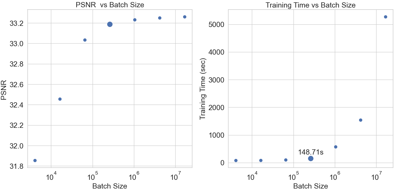
Figure 17: The graph showcases the impact of batch size on PSNR (LHS) and training time (RHS). Various learning rates from $[0.0001,0.1]$ were tested, and the optimal rate for each batch size was identified. The training spanned over 4096 iterations with upsampling steps at intervals $[64,128,256,512,1024]$. The batch size of $512^{2}$, highlighted in the figure, was selected for its optimal balance between high accuracy and time efficiency, as evidenced in the training of the 4k ”Girl with a Pearl Earring” image with a rank of 200.

Fig. 17 illustrates these relationships, displaying how different batch sizes influenced both the PSNR and the training time in our experiments with a 4k ”Girl with a Pearl Earring” image using a PuTT.

F.2 Learning Rate Strategy in Training Process

In our training setup, we implement an exponential learning rate decay strategy with a decay factor of $\alpha=0.1$. This decay reduces the learning rate exponentially by $\alpha$ between upsampling iterations. For example, if upsampling occurs at iteration $1000$, the learning rate declines from $5\cdot 10^{-3}$ to $\alpha\cdot 5\cdot 10^{-3}=5\cdot 10^{-4}$ from step $0$ to step $1000$.

We observe a characteristic pattern in the loss behavior post-upsampling: an initial spike in loss due to the introduction of higher-resolution interpolations. As the number of parameters in the representation increases, a new optimizer with an adjusted learning rate is necessary. Simply maintaining the pre-upsampling learning rate leads to minimal loss reduction, potentially trapping the model in local minima. Conversely, resetting to the base learning rate causes significant loss fluctuations.

To address this, we employ a $\beta$ upsampling learning rate decay, where $\beta=0.9$. Post-upsampling, the learning rate is recalibrated to $0.9^{l}\cdot 5\cdot 10^{-3}$ (where $l$ is the number of upsampling steps completed), ensuring a balanced approach between loss stability and effective learning. Following this, we introduce a 50-iteration warm-up phase for the learning rate after each upsampling, enhancing the stability of the training process. Finally, post the last upsampling step, the learning rate undergoes another exponential decay of $\alpha$ until the final iteration, ensuring a smooth convergence towards the end of the training.

F.3 Compression

In Fig. 18,19 we see the SSIM results for our 2D and 3D compression experiments that complements Fig. 6 and 7 (PSNR results) of the main text. Similarly to the PSNR results, we see that PuTT outperform baselines for both 2D and 3D.

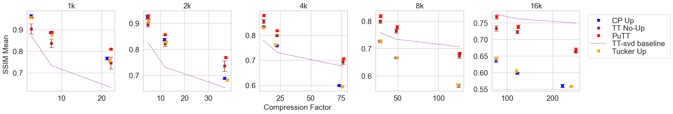
Figure 18: SSIM (y-axis) vs compression ratio (x-axis) for 2D fitting. “up = upsampling”.

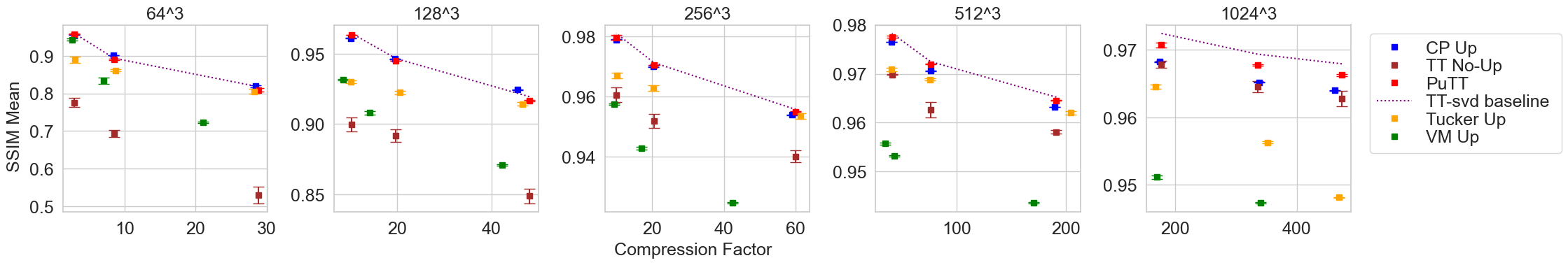
Figure 19: (a) SSIM (y-axis) in comparison to compression ratio (x-axis) for 3D fitting.

F.4 Noise Removal

In Sec. 5.3 of the main text, we evaluate PuTT’s proficiency in learning from noisy samples, comparing it with various tensor network methods and QTTs without upsampling. We aim to learn a tensor representation of a target, denoted as $\mathcal{X}_{I}$, using samples from its noisy counterpart, $\hat{\mathcal{X}}_{I}$, obtained by This noisy version has an identical structure to $\mathcal{X}_{I}$ and is generated by adding noise $Z$. In our experiments, $Z$ is sampled from either a Normal or Laplacian distribution, $Z\sim\mathcal{N}(0,\sigma)$, or a Laplacian distribution, $Z\sim\text{Laplace}(0,b)$. Thus, the noisy target is formulated as $\hat{\mathcal{X}}_{I}=\mathcal{X}_{I}+Z$.

In Sec. 5.3 of the main text, Figures 10 (a) and (b) present quantitative results for noise resilience in 2D focusing on PSNR and SSIM metrics. In the 3D noise resilience analysis (Figures 20 and 21), PuTT mirrors its 2D success, maintaining higher PSNR against other methods across various noise levels. Upsampling significantly boosts performance, especially in SSIM metrics for noise above $0.2\sigma$, demonstrating PuTT’s strong noise handling capabilities in both 2D and 3D scenarios.

For our Noise Removal experiments, we adjust the learning rate to accommodate varying noise levels. Starting with an initial learning rate of $lr_{init}=0.005$ at zero noise, we modify this rate for both PuTT and baseline methods according to the formula $lr_{\sigma}=0.005\times 0.1^{\sigma}$, where $0.1$ is our chosen adaptation factor. For instance, at a noise level of $\sigma=0.5$, the learning rate becomes $lr_{\sigma}=0.005\times 0.1^{0.5}\approx 0.00158$. This approach helps in achieving optimal results across different noise intensities.

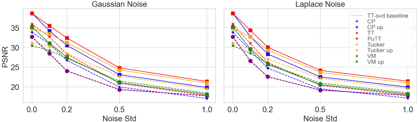
Figure 20: PSNR when varying the amount of Gaussian or Laplacian noise for PuTT and baselines for 3D experiments. “up = upsampling”.

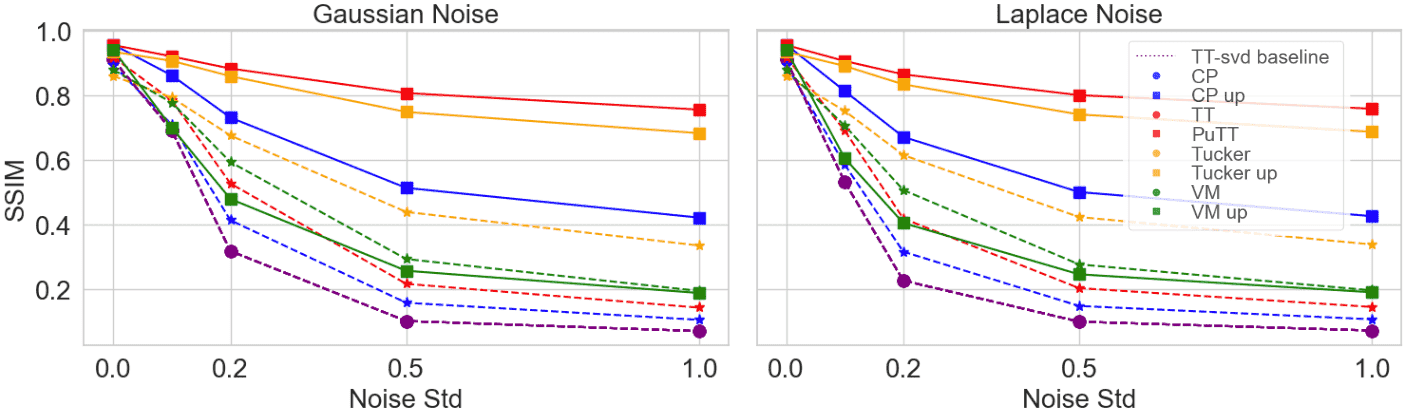
Figure 21: Same as Fig. 20 but for SSIM

F.5 Incomplete Data Experiments

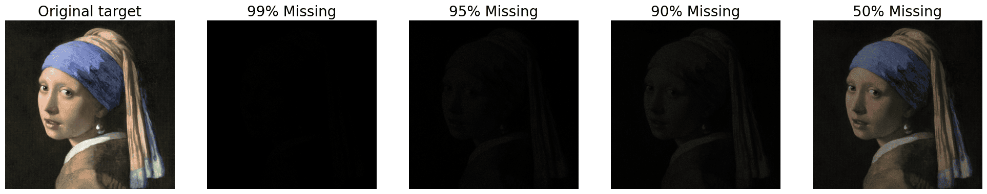
(a) Original and Incomplete Images

Figure 22: Incomplete data training inputs for various Percentages: The sequence starts with the original target image (leftmost), followed by the varying percentages of missing data from 99% to 50%.

In Sec. 5.2 of the main text, we presented the results for training on limited data for various percentages. Fig. 22 presents the training data used in training at various percentages. The sequence begins with the original target image, followed by its version with a percentage of the original data sampled. These versions are created by randomly setting a specified percentage of the pixels in the original image to zero, representing scenarios with limited data availability. The subsampling percentages, ranging from 1% to 50%, are specified above each corresponding image.

In Sec. 5.2 of the main text, Fig. 12 shows how varying the number of upsampling steps when training $99\%$ missing data affects PSNR and SSIM for ”Girl with Pearl Earrings” 4k. The first image displays the training data, followed by PuTT results with $0,1,4$, and $7$ upsampling steps. Fig. 23 shows the larger visual examples.

In our Incomplete Data experiments, similar to the Noise Removal experiments, we modify the learning rate based on the proportion of available training data. We observed that optimal results were achieved with lower learning rates when less training data was accessible. Initially, we set the learning rate to $lr_{init}=0.005$ when all data points are available. As the amount of training data decreases, we adjust the learning rate for PuTT and baseline methods using the formula $lr_{p}=0.005\times f^{1-p}$. Here, $f$ represents the adaptation factor, and $p$ denotes the proportion of available training data, ranging between 0 and 1. This strategy helps us tailor the learning process effectively to different data availability scenarios.

Figure 23: Varying the number of upsampling steps when training $99\%$ missing data. The first image displays the training data, followed by PuTT results with $0,1,4$, and $7$ upsampling steps.

Downsampled images  Fig. 24 shows the downsampled targets used during training for $95\%$ missing data of ”Girl with Pearl Earring”. The three RGB channels are averaged to visualize how aggregated values form a blurred version of the actual target at lower downsampled resolutions.

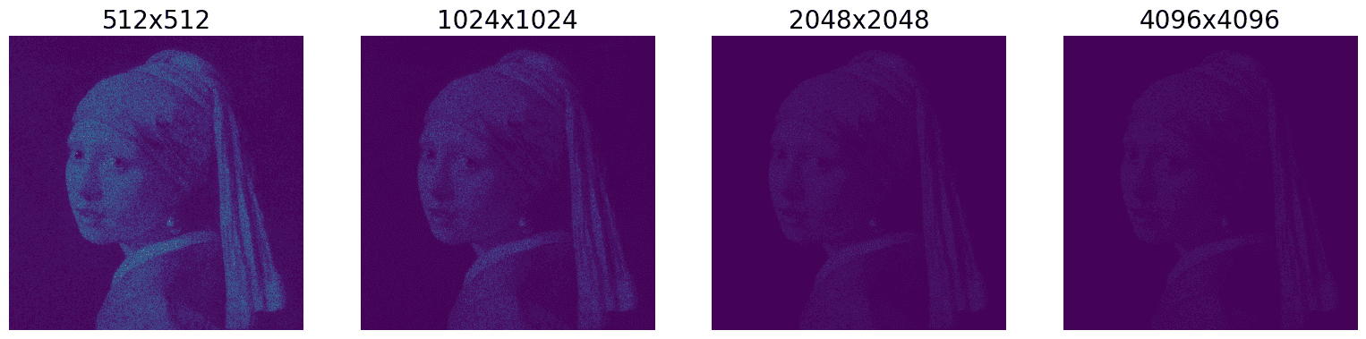
Figure 24: Illustration of the effects of downsampling a 4k image where $95\%$ of the data at the target resolution is missing. The progression from left to right shows images at lower resolutions containing aggregated information about the pixels available at higher resolutions. The three channels have been aggregated to more clearly show this pattern

Masked average pooling  As explained in Sec. 5.2 of the main text, to train with a downsampled target at lower resolutions, we create a modified target image $I_{D-l,p}$. We build $I_{D-1,p}$ from $I_{D,p}$, we use a custom masked average pooling method, averaging only the non-zero values in each window, sized according to the downsampling factor. The masked average pooling can be illustrated through a simple example. Consider a $2\times 2$ window containing values $[2,2,0,0]$. In standard average pooling, the output would be the average of all values, $(2+2+0+0)/4=1$. However, in our masked average pooling, where zero values are excluded from the calculation, the output is the average of the non-zero values, $(2+2)/2=2$. This method ensures that only relevant data contributes to the pooling process. Fig. 24 provides a visual representation of this process. It showcases how a 4k image, with 95% of its data missing at the target resolution, is progressively downsampled. Each image in the sequence, moving from left to right, represents a lower-resolution version, consolidating aggregated information from the available pixels at higher resolutions. For easier visualization, the channel dimension has been averaged.

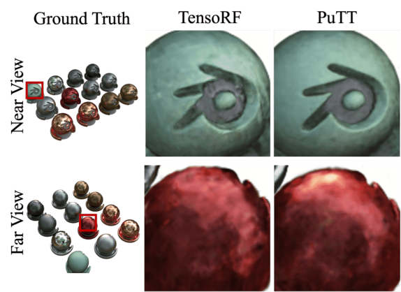
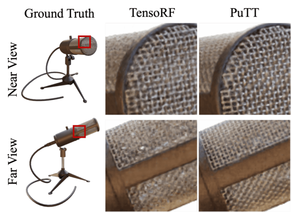
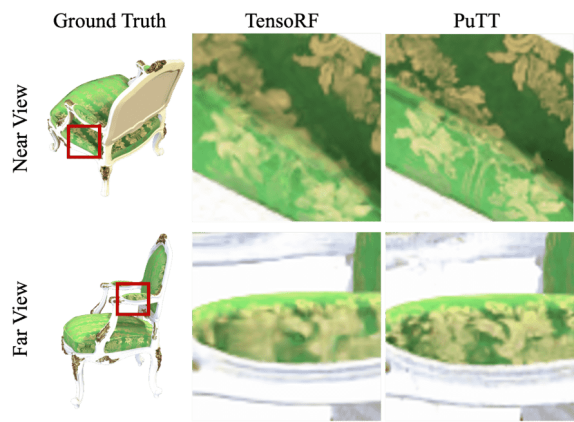
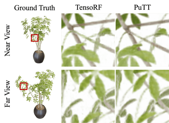
Figure 25: Visual comparison of TensoRF and PuTT on Near and Far views for “Materials”, “Mic”, “Chair”, “Ficus” scenes.

Appendix G Novel View Synthesis

Model (Size)	PSNR	SSIM	LPIPS
PuTT (12 MB)	31.953	0.957	0.0597
PuTT (12 MB) No PE	31.880	0.9537	0.0612
PuTT (12 MB) No Up	31.466	0.9502	0.0654
TensoRF (12 MB)	31.623	0.9523	0.0626
PuTT (7 MB)	31.665	0.9560	0.0602
PuTT (7 MB) No PE	31.633	0.9516	0.0650
PuTT (7 MB) No UP	31.295	0.9480	0.0710
TensoRF (7 MB)	31.103	0.9476	0.0697

Table 5: Comparison of novel view synthesis (NeRF) under different model sizes (7MB and 12MB) in comparison to TensoRF. ”No Up”: No upsampling, ”No PE”: No positional encoding used for inputs to the Shader (MLP) function.

We compare our approach with other grid-based novel view synthesis methods, including previous works NSVF (Liu et al., 2020a) PlenOctrees (Yu et al., 2021b), Plenoxels (Yu et al., 2021a), DVGO (Sun et al., 2022), K-planes (Fridovich-Keil et al., 2023), and TensoRF (Chen et al., 2022). Most of these results were taken directly from the respective papers if possible. We directly compare the tensor methods used by TensoRF and their efficiency vs our PuTT method’s effeciency, by aligning the model sizes of the two. In our comparison with TensoRF, we omitted its ”shrinkage” feature, which involves using an alpha mask to dynamically reshape and resample tensor factors during training. However, due to its current incompatibility with our QTT structure, integrating this feature into PuTT requires additional development. Instead, in our experiments, we employed a progressively updated alpha mask, utilized exclusively for ray-filtering purposes. This adjustment was critical in maintaining a fair and relevant comparison between the methods under test.

In our novel view synthesis experiments, models were trained for a total of $80,000$ steps. The learning rate (LR) schedule followed the same structure as outlined in Sec. 5.1 of the main text, but for PuTT, we used a base LR of $1e-3$. In the case of TensoRF, we adhered to its standard configuration but adjusted the factor counts in the VM decomposition to align with our 7MB and 12MB model sizes. For the 7MB TensoRF models, the rank factors were set to $[4,4,4]$ for density and $[5,5,5]$ for appearance. In contrast, for the larger 12MB models, we increased these ranks to $[8,8,8]$ for both density and appearance factors, ensuring a consistent comparison in terms of memory footprint. For PuTT 7MB is equal to a rank of $140$ for the density grid and $200$ for the appearance grid, and for the 12MB model, this is $200$ and $280$ respectively.

Regarding batch sizes, our experiments utilized $4096$ rays per batch. The number of uniform samples per ray was capped at $884$. Both models, PuTT and TensoRF, demonstrated similar running times, ranging between 4 and 5 hours for both 7MB and 12MB on an NVIDIA Tesla V100 GPU. The increased running time observed with TensoRF compared to those reported in their paper can be attributed to not employing its shrinkage feature. While this feature typically enhances efficiency in TensoRF’s processing, its exclusion was necessary to ensure a more direct comparison with the PuTT model under equivalent conditions.

We assessed our method under different conditions: with and without Positional Encoding (PE), and with and without Upsampling, applied to both the 7MB and 12MB model sizes. Additionally, these configurations were contrasted with TensoRF, both with and without its Upsampling feature. Each experiment was replicated over three seeds to ensure robustness, with the outcomes detailed in Tab. 5.

G.1 Omitting Positional Encoding

One of the key innovations in the original NeRF (Mildenhall et al., 2020) was the use of Positional Encoding (PE) to transform 5D input coordinates into a higher-dimensional space, enhancing the representation of high-frequency scene content. This technique resulted in a significant PSNR improvement for NeRF (Mildenhall et al., 2020). Our findings, as shown in Tab. 5, suggest that the quantized TT structure effectively encodes inputs for the MLP responsible for color value computations based on viewing directions. With the quantized TT structure, we observed only a minor drop in performance when PE was omitted. For the 12MB model, we only see a drop of $0.07$ PSNR when not using Positional Encoding as opposed to the drop reported by Mildenhall et al. in NeRF (Mildenhall et al., 2020), which was a difference of $2.24$ PSNR. This highlights the effectiveness of the quantized tensor train encoding.

G.2 Testing from Near to Far Views

Metric	Method	Chair		Drums		Ficus		Hotdog		Lego		Materials		Mic		Ship		Average
		TensoRF	PuTT	TensoRF	PuTT	TensoRF	PuTT	TensoRF	PuTT	TensoRF	PuTT	TensoRF	PuTT	TensoRF	PuTT	TensoRF	PuTT	TensoRF	PuTT
PSNR	Near	35.953	37.450	27.024	27.672	32.653	34.254	37.176	38.276	34.396	35.579	28.915	29.309	33.510	34.886	30.463	30.990	32.511	33.552
	Far	31.798	33.262	24.444	24.951	30.457	31.822	31.579	31.331	31.434	31.523	25.986	26.177	33.515	34.382	27.287	27.264	29.563	30.089
	All	32.616	34.144	25.004	25.444	30.986	32.253	36.034	36.590	33.264	34.009	28.953	29.331	32.520	33.596	29.128	29.559	31.063	31.866

Table 6: Novel View Synthesis comparison to TensoRF (PSNR) for all scenes in the Synthetic-NeRF (Mildenhall et al., 2020) dataset. We test on views that are near training views (Near), far from training views (Far), and all test views (All). The models being compared have a size og 7MB.

To study the fine-grained representation ability of PuTT, we experiment with testing views captured from near to far camera positions compared with source views. Specifically, we compute the average variance in view angles between each testing view and its nearest twenty source views. After sorting the average view angle differences for all testing views, we identify the twenty testing views with the smallest differences as near views and the twenty testing views with the largest differences as far views.

In addition to Sec. 5.1 of the main text, Tab. 6 shows that PuTT outperforms TensorRF from near to far testing views on both SSIM and LPIPS for all scenes in the dataset. It should be noticed that the advantage of PuTT over TesorRF on near views is more significant than that on far views. It indicates that PuTT, benefiting from the coarse-to-fine learning method, learns a more compact and expressive representation of the fine-grained details, as shown in Fig. 25.

G.3 Per-scene results novel view synthesis

Methods	Avg.	Chair	Drums	Ficus	Hotdog	Lego	Materials	Mic	Ship
PSNR$\uparrow$
PlenOctrees-L* (Yu et al., 2021b)	31.71	34.66	25.31	30.79	36.79	32.95	29.76	33.97	29.42
Plenoxels-L* (Yu et al., 2021a)	31.71	33.98	25.35	31.83	36.43	34.10	29.14	33.26	29.62
DVGO-L* (Sun et al., 2022)	31.95	34.09	25.44	32.78	36.74	34.64	29.57	33.20	29.13
kplanes-L* (Fridovich-Keil et al., 2023)	32.36	34.99	25.66	31.41	36.78	35.75	29.48	34.05	30.74
Instant-NGP* (Müller et al., 2022)-L	33.18	35.00	26.02	33.51	37.40	36.39	29.78	36.22	31.10
TensoRF VM-192-L* (Chen et al., 2022)	33.14	35.76	26.01	33.99	37.41	36.46	30.12	34.61	30.77
Our PuTT-200-L	32.79	35.29	25.82	33.39	37.29	35.93	29.93	34.21	30.39
NeRF-S* (Mildenhall et al., 2020)	31.01	33.00	25.01	30.13	36.18	32.54	29.62	32.91	28.65
TensoRF VM-30-S (no shrinking)	31.10	32.62	25.00	30.99	36.03	33.26	28.95	32.52	29.13
Our PuTT-200-S	31.87	34.14	25.44	32.25	36.59	34.01	29.33	33.60	29.56
Instant-NGP-M* (Müller et al., 2022)	33.17	35.00	26.02	33.51	37.40	36.39	29.78	36.22	31.10
TensoRF VM-48-M (no shrinking)	31.51	33.29	25.22	31.62	36.24	33.79	29.34	32.97	29.59
Our PuTT-200-M	31.98	34.23	25.67	32.32	37.07	34.02	29.58	33.56	29.44
SSIM$\uparrow$
PlenOctrees-L* (Yu et al., 2021b)	0.958	0.981	0.933	0.970	0.982	0.971	0.955	0.987	0.884
Plenoxels-L* (Yu et al., 2021a)	0.958	0.977	0.933	0.976	0.980	0.976	0.949	0.985	0.890
DVGO-L* (Sun et al., 2022)	0.957	0.977	0.930	0.978	0.980	0.976	0.951	0.983	0.879
kplanes-L* (Fridovich-Keil et al., 2023)	0.962	0.983	0.938	0.975	0.982	0.982	0.950	0.988	0.897
TensoRF VM-192-L* (Chen et al., 2022)	0.963	0.985	0.937	0.982	0.982	0.983	0.952	0.988	0.895
Our PuTT-600-L	0.958	0.977	0.933	0.979	0.981	0.972	0.947	0.986	0.888
NeRF-S* (Mildenhall et al., 2020)	0.947	0.967	0.925	0.964	0.974	0.961	0.949	0.980	0.856
TensoRF VM-30-S (no shrinking)	0.948	0.965	0.920	0.966	0.974	0.966	0.938	0.979	0.873
Our PuTT-200-S	0.956	0.976	0.928	0.975	0.979	0.974	0.945	0.987	0.876
TensoRF VM-48-M (no shrinking)	0.952	0.971	0.923	0.969	0.975	0.974	0.944	0.982	0.879
Our PuTT-280-M	0.957	0.976	0.929	0.975	0.979	0.973	0.946	0.989	0.878
LPIPS${}_{Vgg}\downarrow$
DVGO-L* (Sun et al., 2022)	0.035	0.016	0.061	0.015	0.017	0.014	0.026	0.014	0.118
TensoRF VM-192-L* (Chen et al., 2022)	0.027	0.010	0.051	0.012	0.013	0.007	0.026	0.009	0.085
Our PuTT-600-L	0.045	0.021	0.081	0.025	0.019	0.027	0.045	0.018	0.124
NeRF-S* (Mildenhall et al., 2020)	0.081	0.046	0.091	0.044	0.121	0.050	0.063	0.028	0.206
TensoRF VM-30-S (no shrinking)	0.067	0.042	0.104	0.034	0.042	0.039	0.074	0.025	0.177
Our PuTT-200-S	0.061	0.037	0.085	0.029	0.038	0.039	0.069	0.024	0.161
TensoRF VM-48-M (no shrinking)	0.062	0.041	0.100	0.032	0.0412	0.037	0.072	0.022	0.155
Our PuTT-280-M	0.059	0.034	0.084	0.029	0.037	0.039	0.069	0.022	0.158

Table 7: Quantitative results on each scene from the Synthetic-NeRF (Mildenhall et al., 2020) dataset. (Results denoted with an asterisk (*) were sourced from the data presented in the referenced paper.

Methods	Avg.	Wineholder	Steamtrain	Toad	Robot	Bike	Palace	Spaceship	Lifestyle
PSNR$\uparrow$
DVGO-L* (Sun et al., 2022)	35.08	30.26	36.56	33.10	36.36	38.33	34.49	37.71	33.79
TensoRF VM-192-L* (Chen et al., 2022)	36.52	31.32	37.87	34.85	38.26	39.23	37.56	38.60	34.51
Our PuTT-600-L	36.57	31.33	37.21	34.87	38.22	39.32	37.47	39.07	35.05
NeRF-S* (Mildenhall et al., 2020)	30.81	28.23	30.84	29.42	28.69	31.77	31.76	34.66	31.08
TensoRF VM-30-S (no shrinking)	34.58	29.62	35.51	32.21	35.42	37.85	35.49	37.05	33.48
Our PuTT-200-S	35.59	30.55	36.22	33.73	36.44	38.59	36.02	38.72	34.43
TensoRF VM-48-M (no shrinking)	35.41	30.35	36.54	32.84	36.85	38.33	36.54	37.51	34.34
Our PuTT-280-M	36.04	30.89	36.41	34.48	37.02	38.89	36.78	38.95	34.86
SSIM$\uparrow$
DVGO-L* (Sun et al., 2022)	0.975	0.949	0.989	0.966	0.992	0.991	0.962	0.988	0.965
TensoRF VM-192-L* (Chen et al., 2022)	0.982	0.961	0.991	0.978	0.994	0.993	0.979	0.989	0.968
Our PuTT-600-L	0.982	0.960	0.989	0.979	0.994	0.993	0.977	0.990	0.970
NeRF-S* (Mildenhall et al., 2020)	0.952	0.920	0.966	0.920	0.960	0.970	0.950	0.980	0.946
TensoRF VM-30-S (no shrinking)	0.974	0.949	0.985	0.962	0.992	0.991	0.970	0.982	0.962
Our PuTT-200-S	0.976	0.954	0.985	0.971	0.990	0.989	0.968	0.989	0.965
TensoRF VM-48-M (no shrinking)	0.975	0.949	0.986	0.963	0.992	0.991	0.973	0.985	0.964
Our PuTT-280-M	0.977	0.956	0.983	0.974	0.990	0.990	0.975	0.984	0.967
LPIPS${}_{VGG}\downarrow$
DVGO-L* (Sun et al., 2022)	0.019	0.038	0.010	0.030	0.005	0.004	0.027	0.009	0.027
TensoRF-VM-192-L* (Chen et al., 2022)	0.012	0.024	0.006	0.016	0.003	0.003	0.011	0.009	0.021
Our PuTT-600-L	0.017	0.032	0.017	0.023	0.008	0.004	0.021	0.011	0.023
NeRF-S* (Mildenhall et al., 2020)	0.043	0.096	0.031	0.069	0.038	0.019	0.031	0.016	0.047
TensoRF VM-30-S (no shrinking)	0.036	0.059	0.032	0.046	0.014	0.017	0.033	0.027	0.057
Our PuTT-200-S	0.032	0.059	0.029	0.039	0.013	0.014	0.032	0.018	0.055
TensoRF VM-48-M (no shrinking)	0.034	0.065	0.028	0.043	0.013	0.014	0.029	0.025	0.056
Our PuTT-280-M	0.027	0.053	0.022	0.031	0.011	0.011	0.024	0.017	0.046

Table 8: Quantitative results on each scene from the Synthetic-NSVF (Liu et al., 2020a) dataset. Results denoted with an asterisk (*) were sourced from the data presented in the referenced paper.

Methods	Avg.	Ignatius	Truck	Barn	Caterpillar	Family
PSNR$\uparrow$
PlenOctrees-L* (Yu et al., 2021b)	27.99	28.19	26.83	26.80	25.29	32.85
Plenoxels-L* (Yu et al., 2021a)	27.43	27.51	26.59	26.07	24.64	32.33
DVGO-L* (Sun et al., 2022)	28.41	28.16	27.15	27.01	26.00	33.75
TensoRF VM-192-L (Chen et al., 2022)	28.56	28.34	27.14	27.22	26.19	33.92
Our PuTT-600-L	28.37	28.08	27.09	27.22	25.93	33.56
NeRF-S* (Mildenhall et al., 2020)	25.78	25.43	25.36	24.05	23.75	30.29
TensoRF VM-30-S (no shrinking)	27.67	27.58	26.42	26.67	25.04	32.62
Our PuTT-200-S	27.99	27.98	26.47	27.08	25.47	32.96
TensoRF VM-48-M (no shrinking)	28.03	28.04	26.70	27.06	25.28	33.06
Our PuTT-280-M	28.15	28.01	26.91	27.01	25.61	33.23
SSIM$\uparrow$
PlenOctrees-L* (Yu et al., 2021b)	0.917	0.948	0.914	0.856	0.907	0.962
Plenoxels-L* (Yu et al., 2021a)	0.906	0.943	0.901	0.829	0.902	0.956
DVGO-L* (Sun et al., 2022)	0.911	0.944	0.906	0.838	0.906	0.962
TensoRF VM-192-L* (Chen et al., 2022)	0.920	0.948	0.914	0.864	0.912	0.965
Our PuTT-600-L	0.917	0.943	0.908	0.865	0.907	0.960
NeRF-S* (Mildenhall et al., 2020)	0.864	0.920	0.860	0.750	0.860	0.932
TensoRF VM-30-S (no shrinking)	0.899	0.924	0.900	0.840	0.880	0.951
Our PuTT-200-S	0.901	0.931	0.901	0.824	0.901	0.950
TensoRF VM-48-M (no shrinking)	0.901	0.928	0.900	0.843	0.882	0.951
Our PuTT-280-M	0.907	0.934	0.909	0.835	0.903	0.953
LPIP${}_{VGG}\downarrow$
DVGO-L* (Sun et al., 2022)	0.148	0.090	0.145	0.290	0.152	0.064
TensoRF VM-192-L* (Chen et al., 2022)	0.140	0.078	0.145	0.252	0.159	0.064
Our PuTT-600-L	0.142	0.082	0.153	0.241	0.163	0.070
NeRF-S* (Mildenhall et al., 2020)	0.198	0.111	0.192	0.395	0.196	0.098
TensoRF VM-30-S (no shrinking)	0.185	0.099	0.218	0.297	0.227	0.083
Our PuTT-200-S	0.197	0.094	0.326	0.272	0.220	0.072
TensoRF VM-48-M (no shrinking)	0.156	0.092	0.173	0.257	0.187	0.074
Our PuTT-280-M	0.150	0.086	0.162	0.259	0.170	0.073

Table 9: Quantitative results on each scene from the Tanks&Temples (Knapitsch et al., 2017) dataset. Results denoted with an asterisk (*) were sourced from the data presented in the referenced paper.

Appendix H Compatibility of TensoRF’s ”Shrinkage” with QTT

Shrinkage: TensoRF’s “shrinkage” process removes parameters corresponding to empty regions in the 3D space. For instance, in TensoRF’s VM (Vector-Matrix) decomposition, parameters for indices $x,y,z<10$ are pruned if the region is empty, reallocating them to denser regions to enhance resolution.

Incompatibility with QTT: Unlike TensoRF, QTT uses a hierarchical structure with mode quantization, compressing dimensions into powers of two. This structure mixes parameters, interlinking those representing a coordinate $(x,y,z)$ with many others. Consequently, QTT’s parameter sharing across the hierarchy complicates direct pruning as in TensoRF’s “shrinkage.” Figure 16 illustrates this interlinked structure. While QTT’s interdependency complicates “shrinkage,” it allows capturing dimensional correlations, ensures logarithmic parameter growth, and improves robustness against noise and incomplete data. Updating parameters for a specific coordinate refines those across interconnected indices, leveraging correlations for resilient data representation. This complexity necessitates a coarse-to-fine training approach, as proposed in our PuTT method, fostering the hierarchical structure modeled by QTT.

Appendix I Exploring Inpainting Capabilities with PuTT

Inpainting tasks benefit from a rich prior of the true data distribution, often using generative models. Our method, however, focuses on a single example to learn a compact, high-quality representation suitable for tasks like denoising or predicting missing values.

We conducted an experiment with two images: a brick pattern and the Lena image. Each image had a continuous mask covering 10% of the area. Using PuTT, we attempted to reconstruct the masked regions. Results are shown in Fig. 26 with columns for the original image, the masked image, and the reconstructed image. The brick image shows PuTT’s effectiveness in structured settings, while the Lena image highlights the challenges of inpainting large areas without sophisticated priors.

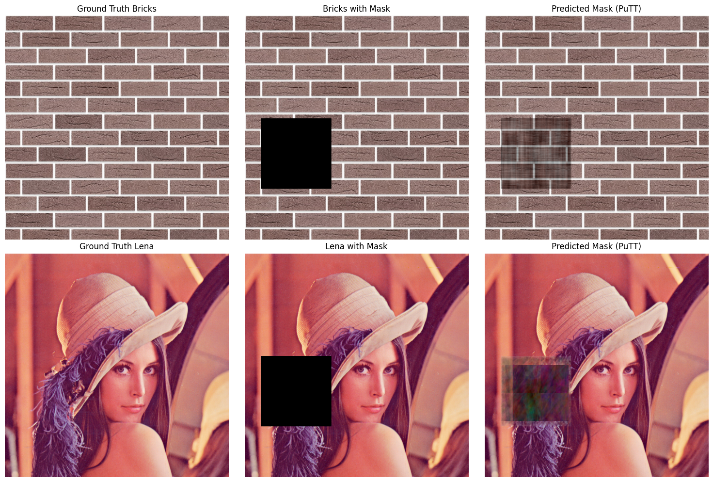
Figure 26: Inpainting results on two $512\times 512\times 3$ images: a brick pattern (top) and the Lena image (bottom). Columns display the original image, the masked image (10% mask), and the PuTT reconstruction. Reconstructions were achieved after 1024 iterations using only unmasked regions.

Appendix J Exploring Rank Incrementation with SlimmeRF

SlimmeRF (Yuan & Zhao, 2023) enhances the TensoRF VM framework by introducing an adaptive rank mechanism, dynamically adjusting the model’s learning capacity. The model starts with a low-rank representation and incrementally increases the rank based on learning progress, capturing essential features early and building complexity as needed. Our approach similarly increases tensor rank progressively, a strategy used in physics methods like DMRG (White, 1992a) and TT-cross (Oseledets & Tyrtyshnikov, 2010), aligning with our progressive learning in PuTT.

We explored this with a 2D compression experiment on 4K images, as shown in Table 10. We compared a standard QTT model without upsampling to one with progressive rank incrementation ([2, 4, 8, 16] ranks during initial training). These experiments indicate that gradual rank increments can improve PSNR scores without adding complexity.

These results, excluding dimensional upsampling, highlight the potential of rank incrementation. However, more extensive experiments are needed to fully validate these findings.

Rank Increment	PSNR (Avg)	Std
0 (Baseline)	37.444	0.821
2	38.168	0.391
4	38.273	0.444
8	38.331	0.464
16	38.131	0.513

Table 10: Results of Progressive Rank Incrementation. This table summarizes the effects of rank incrementation on learning efficiency for a 1k resolution image of a ’Girl with a Pearl Earring’. It contrasts a baseline QTT model without upsampling, starting with a rank of $200$, with QTT models employing progressive rank incrementation from a base rank of $100$ to $200$. Rank increments of $2$, $4$, $8$, and $16$ were tested over four intervals: $[100,1000],[100,1500],[250,1500]$, and $[250,750]$, to determine the start and end points for rank increments. The table displays the average PSNR values, alongside standard deviations, across three iterations for each rank increment strategy. These results highlight the improved performance due to strategic rank incrementation, with all strategies surpassing the baseline. For instance, an increment step of $2$ within the $[100,1000]$ interval increased the rank every $(1000-100)/(200-100)=9$ iterations. Although a rank increment of 8 yielded the best average PSNR, differences between increment steps were minimal, suggesting a thoughtful approach to rank incrementation can significantly enhance the model’s learning capability.

References

- Adelson et al. (1984) Adelson, E. H., Anderson, C. H., Bergen, J. R., Burt, P. J., and Ogden, J. M. Pyramid methods in image processing. RCA engineer, 29(6):33–41, 1984.
- Antonini et al. (1990) Antonini, M., Barlaud, M., Mathieu, P., and Daubechies, I. Image coding using vector quantization in the wavelet transform domain. In International Conference on Acoustics, Speech, and Signal Processing, pp. 2297–2300 vol.4, 1990. doi: 10.1109/ICASSP.1990.116036.
- Bramble (2019) Bramble, J. H. Multigrid methods. Chapman and Hall/CRC, 2019.
- Carroll & Chang (1970) Carroll, J. D. and Chang, J. J. Analysis of individual differences in multidimensional scaling via an n-way generalization of “eckart-young” decomposition. Psychometrika, 35:283–319, 1970. URL https://api.semanticscholar.org/CorpusID:50364581.
- Chan et al. (2021) Chan, E. R., Monteiro, M., Kellnhofer, P., Wu, J., and Wetzstein, G. pi-gan: Periodic implicit generative adversarial networks for 3d-aware image synthesis. In Proceedings of the IEEE/CVF conference on computer vision and pattern recognition, pp. 5799–5809, 2021.
- Chan et al. (2022) Chan, E. R., Lin, C. Z., Chan, M. A., Nagano, K., Pan, B., De Mello, S., Gallo, O., Guibas, L. J., Tremblay, J., Khamis, S., et al. Efficient geometry-aware 3d generative adversarial networks. In Proceedings of the IEEE/CVF Conference on Computer Vision and Pattern Recognition, pp. 16123–16133, 2022.
- Chen et al. (2022) Chen, A., Xu, Z., Geiger, A., Yu, J., and Su, H. Tensorf: Tensorial radiance fields, 2022. URL https://arxiv.org/abs/2203.09517.
- Crowley & Stern (1984) Crowley, J. L. and Stern, R. M. Fast computation of the difference of low-pass transform. IEEE transactions on pattern analysis and machine intelligence, 1(2):212–222, 1984.
- Dobson (2018) Dobson, T. 1.2 gigapixel panorama of shibuya in tokyo, japan. https://www.flickr.com/photos/trevor_dobson_inefekt69/29314390837, 2018. Accessed: 17-11-2023.
- Fridovich-Keil et al. (2023) Fridovich-Keil, S., Meanti, G., Warburg, F., Recht, B., and Kanazawa, A. K-planes: Explicit radiance fields in space, time, and appearance, 2023.
- Harshman (1970) Harshman, R. A. Foundations of the PARAFAC procedure: Models and conditions for an ”explanatory” multi-modal factor analysis. UCLA Working Papers in Phonetics, 16:1–84, 1970.
- Holtz et al. (2012) Holtz, S., Rohwedder, T., and Schneider, R. The alternating linear scheme for tensor optimization in the tensor train format. SIAM Journal on Scientific Computing, 34(2):A683–A713, 2012.
- Hubig et al. (2017) Hubig, C., McCulloch, I. P., and Schollwoeck, U. Generic construction of efficient matrix product operators. Phys. Rev. B, 95:035129, Jan 2017. doi: 10.1103/PhysRevB.95.035129. URL https://link.aps.org/doi/10.1103/PhysRevB.95.035129.
- Khoromskij (2011) Khoromskij, B. N. -quantics approximation of n-d tensors in high-dimensional numerical modeling. Constructive Approximation, 34:257–280, 2011.
- Kingma & Ba (2014) Kingma, D. P. and Ba, J. Adam: A method for stochastic optimization. arXiv preprint arXiv:1412.6980, 2014.
- Klümper et al. (1993) Klümper, A., Schadschneider, A., and Zittartz, J. Matrix product ground states for one-dimensional spin-1 quantum antiferromagnets. Europhysics Letters, 24(4):293, 1993.
- Knapitsch et al. (2017) Knapitsch, A., Park, J., Zhou, Q.-Y., and Koltun, V. Tanks and temples: benchmarking large-scale scene reconstruction. ACM Trans. Graph., 36(4), jul 2017. ISSN 0730-0301. doi: 10.1145/3072959.3073599. URL https://doi.org/10.1145/3072959.3073599.
- Kolda & Bader (2009) Kolda, T. G. and Bader, B. W. Tensor decompositions and applications. SIAM review, 51(3):455–500, 2009.
- Li et al. (2008) Li, Y., Perlman, E., Wan, M., Yang, Y., Meneveau, C., Burns, R., Chen, S., Szalay, A., and Eyink, G. A public turbulence database cluster and applications to study lagrangian evolution of velocity increments in turbulence. Journal of Turbulence, 9:N31, jan 2008. doi: 10.1080/14685240802376389. URL https://doi.org/10.1080%2F14685240802376389.
- Lindell et al. (2022) Lindell, D. B., Van Veen, D., Park, J. J., and Wetzstein, G. Bacon: Band-limited coordinate networks for multiscale scene representation. In Proceedings of the IEEE/CVF conference on computer vision and pattern recognition, pp. 16252–16262, 2022.
- Liu et al. (2020a) Liu, L., Gu, J., Lin, K. Z., Chua, T.-S., and Theobalt, C. Neural sparse voxel fields. NeurIPS, 2020a.
- Liu et al. (2020b) Liu, L., Gu, J., Lin, K. Z., Chua, T.-S., and Theobalt, C. Neural sparse voxel fields. NeurIPS, 2020b.
- Lombardi et al. (2019) Lombardi, S., Simon, T., Saragih, J., Schwartz, G., Lehrmann, A., and Sheikh, Y. Neural volumes: Learning dynamic renderable volumes from images. arXiv preprint arXiv:1906.07751, 2019.
- Lubasch et al. (2018) Lubasch, M., Moinier, P., and Jaksch, D. Multigrid renormalization. Journal of Computational Physics, 372:587–602, nov 2018. doi: 10.1016/j.jcp.2018.06.065. URL https://doi.org/10.1016%2Fj.jcp.2018.06.065.
- Mallat (1989) Mallat, S. G. A theory for multiresolution signal decomposition: the wavelet representation. IEEE transactions on pattern analysis and machine intelligence, 11(7):674–693, 1989.
- McCulloch (2008) McCulloch, I. Infinite size density matrix renormalization group, revisited. arxiv:0804.2509, 2008. URL https://arxiv.org/abs/0804.2509.
- Mildenhall et al. (2020) Mildenhall, B., Srinivasan, P. P., Tancik, M., Barron, J. T., Ramamoorthi, R., and Ng, R. Nerf: Representing scenes as neural radiance fields for view synthesis. CoRR, abs/2003.08934, 2020. URL https://arxiv.org/abs/2003.08934.
- Müller et al. (2022) Müller, T., Evans, A., Schied, C., and Keller, A. Instant neural graphics primitives with a multiresolution hash encoding. ACM Trans. Graph., 41(4):102:1–102:15, July 2022. doi: 10.1145/3528223.3530127. URL https://doi.org/10.1145/3528223.3530127.
- NASA and ESA (2023) NASA and ESA. Westerlund 2 - nasa and esa, a. nota (esa/stsci), and the westerlund 2 science team. https://hubblesite.org/contents/news-releases/2020/news-2020-15, 2023. Accessed: 17-11-2023.
- NASA/Johns Hopkins University (2023) NASA/Johns Hopkins University. True colors of pluto - from applied physics laboratory/southwest research institute/alex parker. https://science.nasa.gov/resource/true-colors-of-pluto/?category=planets/dwarf-planets_pluto, 2023. Accessed: 17-11-2023.
- Niemeyer & Geiger (2021) Niemeyer, M. and Geiger, A. Giraffe: Representing scenes as compositional generative neural feature fields. In Proceedings of the IEEE/CVF Conference on Computer Vision and Pattern Recognition, pp. 11453–11464, 2021.
- Novikov et al. (2021) Novikov, G. S., Panov, M. E., and Oseledets, I. V. Tensor-train density estimation. In Uncertainty in artificial intelligence, pp. 1321–1331. PMLR, 2021.
- Obukhov et al. (2022) Obukhov, A., Usvyatsov, M., Sakaridis, C., Schindler, K., and Van Gool, L. Tt-nf: Tensor train neural fields, 2022. URL https://arxiv.org/abs/2209.15529.
- Oechsle et al. (2021) Oechsle, M., Peng, S., and Geiger, A. Unisurf: Unifying neural implicit surfaces and radiance fields for multi-view reconstruction. In Proceedings of the IEEE/CVF International Conference on Computer Vision, pp. 5589–5599, 2021.
- of Zurich (2023) of Zurich, U. Computer-assisted paleoanthropology group and visualization and multimedia lab. University of Zurich, 2023. URL https://www.ifi.uzh.ch/en/vmml/research/datasets.html. We acknowledge the Computer-Assisted Paleoanthropology group and the Visualization and MultiMedia Lab at University of Zurich (UZH) for the acquisition of the CT datasets.
- Orús (2019) Orús, R. Tensor networks for complex quantum systems. Nature Reviews Physics, 1(9):538–550, 2019.
- Orús (2014) Orús, R. A practical introduction to tensor networks: Matrix product states and projected entangled pair states. Annals of Physics, 349:117–158, 2014. ISSN 0003-4916. doi: https://doi.org/10.1016/j.aop.2014.06.013. URL https://www.sciencedirect.com/science/article/pii/S0003491614001596.
- Oseledets (2009) Oseledets, I. Approximation of matrices with logarithmic number of parameters. Doklady Mathematics, 80:653–654, 10 2009. doi: 10.1134/S1064562409050056.
- Oseledets & Tyrtyshnikov (2010) Oseledets, I. and Tyrtyshnikov, E. Tt-cross approximation for multidimensional arrays. Linear Algebra and its Applications, 432(1):70–88, 2010. ISSN 0024-3795. doi: https://doi.org/10.1016/j.laa.2009.07.024. URL https://www.sciencedirect.com/science/article/pii/S0024379509003747.
- Oseledets (2011) Oseledets, I. V. Tensor-train decomposition. SIAM Journal on Scientific Computing, 33(5):2295–2317, 2011. doi: 10.1137/090752286. URL https://doi.org/10.1137/090752286.
- Pan & Zhang (2022) Pan, F. and Zhang, P. Simulation of quantum circuits using the big-batch tensor network method. Physical Review Letters, 128(3):030501, 2022.
- Paszke et al. (2019) Paszke, A., Gross, S., Massa, F., Lerer, A., Bradbury, J., Chanan, G., Killeen, T., Lin, Z., Gimelshein, N., Antiga, L., Desmaison, A., Kopf, A., Yang, E., DeVito, Z., Raison, M., Tejani, A., Chilamkurthy, S., Steiner, B., Fang, L., Bai, J., and Chintala, S. Pytorch: An imperative style, high-performance deep learning library. In Advances in Neural Information Processing Systems 32, pp. 8024–8035. Curran Associates, Inc., 2019.
- Perez-Garcia et al. (2007) Perez-Garcia, D., Verstraete, F., Wolf, M. M., and Cirac, J. I. Matrix product state representations, 2007.
- Sitzmann et al. (2019) Sitzmann, V., Thies, J., Heide, F., Nießner, M., Wetzstein, G., and Zollhofer, M. Deepvoxels: Learning persistent 3d feature embeddings. In Proceedings of the IEEE/CVF Conference on Computer Vision and Pattern Recognition, pp. 2437–2446, 2019.
- Stoudenmire (2021) Stoudenmire, E. M. The tensor network, 2021. URL https://tensornetwork.org/mpo. Support for the Tensor Network is provided by the Flatiron Institute, part of the Simons Foundation.
- Studio (2023) Studio, O. . Aerial drone view of urban buildings from top. https://www.pexels.com/@orbital101studio/, 2023. Accessed: 17-11-2023.
- Sun et al. (2022) Sun, C., Sun, M., and Chen, H. Direct voxel grid optimization: Super-fast convergence for radiance fields reconstruction. In CVPR, 2022.
- Szeliski (2022) Szeliski, R. Computer vision: algorithms and applications. Springer Nature, 2022.
- Tucker (1966) Tucker, L. R. Some mathematical notes on three-mode factor analysis. Psychometrika, 31(3):279–311, Sep 1966. ISSN 1860-0980. doi: 10.1007/BF02289464. URL https://doi.org/10.1007/BF02289464.
- Usvyatsov et al. (2022) Usvyatsov, M., Ballester-Ripoll, R., and Schindler, K. tntorch: Tensor network learning with pytorch, 2022.
- Vermeer (1665) Vermeer, J. Girl with a Pearl Earring. https://commons.wikimedia.org/wiki/Category:Girl_with_a_Pearl_Earring_by_Johannes_Vermeer, 1665. Accessed: 17-11-2023.
- Vidal (2007) Vidal, G. Entanglement renormalization. Physical Review Letters, 99(22), nov 2007. doi: 10.1103/physrevlett.99.220405. URL https://doi.org/10.1103%2Fphysrevlett.99.220405.
- White (1992a) White, S. R. Density matrix formulation for quantum renormalization groups. Physical review letters, 69(19):2863, 1992a.
- White (1992b) White, S. R. Density matrix formulation for quantum renormalization groups. Physical review letters, 69(19):2863, 1992b.
- Xie et al. (2022) Xie, Y., Takikawa, T., Saito, S., Litany, O., Yan, S., Khan, N., Tombari, F., Tompkin, J., Sitzmann, V., and Sridhar, S. Neural fields in visual computing and beyond. In Computer Graphics Forum, volume 41, pp. 641–676. Wiley Online Library, 2022.
- Yang et al. (2022) Yang, G., Benaim, S., Jampani, V., Genova, K., Barron, J., Funkhouser, T., Hariharan, B., and Belongie, S. Polynomial neural fields for subband decomposition and manipulation. Advances in Neural Information Processing Systems, 35:4401–4415, 2022.
- Yu et al. (2021a) Yu, A., Fridovich-Keil, S., Tancik, M., Chen, Q., Recht, B., and Kanazawa, A. Plenoxels: Radiance fields without neural networks. CoRR, abs/2112.05131, 2021a. URL https://arxiv.org/abs/2112.05131.
- Yu et al. (2021b) Yu, A., Li, R., Tancik, M., Li, H., Ng, R., and Kanazawa, A. Plenoctrees for real-time rendering of neural radiance fields. CoRR, abs/2103.14024, 2021b. URL https://arxiv.org/abs/2103.14024.
- Yuan & Zhao (2023) Yuan, S. and Zhao, H. Slimmerf: Slimmable radiance fields, 2023.