Simplified and Generalized
Masked Diffusion for Discrete Data

Abstract

Masked (or absorbing) diffusion is actively explored as an alternative to autoregressive models for generative modeling of discrete data. However, existing work in this area has been hindered by unnecessarily complex model formulations and unclear relationships between different perspectives, leading to suboptimal parameterization, training objectives, and ad hoc adjustments to counteract these issues. In this work, we aim to provide a simple and general framework that unlocks the full potential of masked diffusion models. We show that the continuous-time variational objective of masked diffusion models is a simple weighted integral of cross-entropy losses. Our framework also enables training generalized masked diffusion models with state-dependent masking schedules. When evaluated by perplexity, our models trained on OpenWebText surpass prior diffusion language models at GPT-2 scale and demonstrate superior performance on 4 out of 5 zero-shot language modeling tasks. Furthermore, our models vastly outperform previous discrete diffusion models on pixel-level image modeling, achieving 2.78 (CIFAR-10) and 3.42 (ImageNet 64$\times$64) bits per dimension that are comparable or better than autoregressive models of similar sizes.

1 Introduction

Since their inception [1, 2, 3], diffusion models have emerged as the workhorse for generative media, achieving state-of-the-art in tasks such as image synthesis [4, 5, 6], audio [7, 8] and video generation [9, 10, 11, 12, 13]. The majority of existing successes are for continuous state space diffusions. While diffusion models have been extended to discrete state spaces [1, 14, 15] and have been successfully applied to applications ranging from graph generation [16], text-to-sound generation [17] or protein design [18], they remain not as widely used as their continuous counterparts as they are not competitive with autoregressive models in important domains such as text modeling. This has motivated the development of continuous space diffusion models where the discrete data are embedded in the Euclidean space [19, 20, 21, 22, 23] or the simplex [24, 25, 26, 27, 28]. We believe that one of the reasons for the limited success of discrete diffusions is that they have been hindered by fairly complex formulations and training objectives. This paper is a step towards closing this gap.

In this work, we focus on “masked” (or “absorbing”) diffusions, a discrete diffusion formulation first presented by Austin et al. [14], and later explored by the literature from various perspectives [29, 30, 31, 32]. We follow here a continuous-time framework which has proven very useful to improve the training and understanding of continuous state space diffusions [see e.g., 3, 33, 34]. We make several technical contributions which simplify the training of these models and improve significantly their performance. Our contributions are as follows:

• By using elementary arguments, we establish several properties for the forward process induced by this model and its corresponding time reversal, improving our understanding of this model class.

• We provide a remarkably simple expression of the Evidence Lower Bound (ELBO) for masked diffusion models, showing that it corresponds to a weighted integral over time of cross-entropy losses. Similarly to continuous space diffusions [33], this objective can be rewritten in terms of signal-to-noise ratio and exhibits invariance properties.

• We develop a unifying understanding of previously proposed continuous-time discrete diffusion models [29, 35, 32], revealing the changes they made to our ELBO objective and/or model parameterization. We show that these changes either lead to expensive model evaluations, or large variance in training, or breaking the consistency between forward and reverse processes.

• On GPT-2 scale text modeling and pixel-level image modeling tasks, masked diffusions trained using our simple ELBO objective outperform previous proposals, leading to the best likelihood and zero-shot transfer performance among discrete diffusion models.

• Finally, based on our simplified masked diffusion formulation, we propose a generalized masked diffusion model that allows state-dependent masking schedules. This generalized masked diffusion model further improves predictive performance on test likelihoods.

2 Masked Diffusion

Assume our data lives in a finite discrete state space of size $m$. We use the integers $0,1,\dots,m-1$ and their corresponding one-hot vectors $e_{0},e_{1},\dots,e_{m-1}$ to represent the states. In masked diffusion, we augment the space with an additional mask state, which is assigned the index $m$. A forward “masking” process is defined such that a data point is evolved into the mask state at some random time. Reversing this process then gives a generative model of the discrete data.

Discrete-time forward process.

The forward process is defined as a Markovian sequence of discrete random variables $x_{t}$ indexed by time $t$, where $t$ runs from 0 to 1. Throughout the work, we abuse the notation such that $x_{t}$ can be either an integer or its corresponding one-hot vector, whenever it is clear from the context. We divide $[0,1]$ into $T$ intervals, and let $s(i)=(i-1)/T$, $t(i)=i/T$. Following Austin et al. [14], the state transition between $[s(i),t(i)]$ is determined by a transition matrix of size $m\times m$: $Q_{i}=(1-\beta_{i})I+\beta_{i}\mathbf{1}e_{m}^{\top},$ where $\mathbf{1}$ is an all-one vector of size $m+1$, $e_{m}$ represents a one-hot vector with the $m$-th element being 1. Each entry $[Q_{i}]_{jk}$ denotes the probability of transition from the state $j$ to the state $k$:

$$[Q_{i}]_{jk}=q(x_{t(i)}=k|x_{s(i)}=j)=(1-\beta_{i})\delta_{jk}+\beta_{i}\delta_{km}.$$

This means, with probability $1-\beta_{i}$, $x_{t(i)}=x_{s(i)}$, otherwise it jumps to the mask state. Given the above transition matrix, the marginal distribution at time $t(i)$ given $x_{0}$ is

$$q(x_{t(i)}|x_{0})=\mathrm{Cat}(x_{t(i)};\bar{Q}_{i}^{\top}x_{0})=x_{0}^{\top}\bar{Q}_{i}x_{t(i)}.$$

Here, we use $\mathrm{Cat}(x;p)$ to denote a Categorical distribution where $p$ is the vector of probabilities of being in each category, and $\bar{Q}_{i}\triangleq\prod_{j=1}^{i}Q_{j}=\alpha_{i}I+\big{(}1-\alpha_{i}\big{)}\mathbf{1}e_{m}^{\top}$ for $\alpha_{i}=\prod_{j=1}^{i}(1-\beta_{j})$. We expect $\alpha_{T}$ to become very small or zero for a sufficiently large $T$ such that $q(x_{1}|x_{0})$ for any $x_{0}$ will become a delta mass at the mask state.

Continuous-time limit.

We can define a continuous-time forward process by taking a limit of the above discrete-time process. We first specify a continuous function $\beta(t)$ such that $\beta_{i}=\beta(t(i))/T$. We then let $T\to\infty$ in the discrete-time process and compute the limit of $\bar{Q}_{i}$ (proved in Austin et al. 14, Appendix A.6, see also Appendix A and Appendix B) as

$$\bar{Q}(t)\triangleq\lim_{T\to\infty}\bar{Q}_{i} =\alpha_{t}I+(1-\alpha_{t})\mathbf{1}e_{m}^{\top},\text{ where }\alpha_{t}\triangleq\exp\Big{(}-\int_{0}^{t}\beta(s)\mathrm{d}s\Big{)},$$ (1)

so that $q(x_{t}|x_{0})=\mathrm{Cat}(x_{t};\bar{Q}(t)^{\top}x_{0})$. For two arbitrary times, $0\leq s<t\leq 1$, the transition distribution that is compatible with the above marginal (i.e., $q(x_{t}|x_{0})=\sum_{x_{s}}q(x_{t}|x_{s})q(x_{s}|x_{0})$) is

$$q(x_{t}|x_{s}) =\mathrm{Cat}(x_{t};\bar{Q}(s,t)^{\top}x_{s}),\text{ where }\bar{Q}(s,t)\triangleq\bar{Q}(s)^{-1}\bar{Q}(t)=\frac{\alpha_{t}}{\alpha_{s}}I+\big{(}1-\frac{\alpha_{t}}{\alpha_{s}}\big{)}\mathbf{1}e_{m}^{\top}.$$

Note that Austin et al. [14] did not derive this explicit form of transition matrix between two arbitrary time $s$ and $t$, which appeared later in Zhao et al. [36] concurrently with our work.

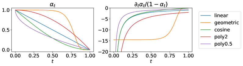
Figure 1: Masking schedules in the literature: (Left) $\alpha_{t}$; (Right) weight of the cross-entropy loss w.r.t. $t$; Equations for these schedules are given in Table 4 in Appendix.

Masking schedules.

From the definition of $\alpha_{t}$, we have that $\alpha_{0}=1$. And similar to the discrete-time formulation, we would like $\alpha_{1}$ be zero or very close to zero. We provide a summary of masking schedules from literature that satisfy these properties in Figure 1. The linear schedule was proposed in Sohl-Dickstein et al. [1] for binary variables and then re-derived by Austin et al. [14] from mutual information for discrete-time models. The geometric schedule $\alpha_{t}$ is plotted for $\bar{\beta}_{\text{min}}=10^{-5}$ and $\bar{\beta}_{\text{max}}=20$. It was first used for continuous diffusions [3] and then for discrete by Lou et al. [32]. The cosine schedule was originally proposed in MaskGIT [30], an iterative unmasking generative model inspired by diffusion. This schedule has the property of slowing down the unmasking process at the beginning of the reverse generation. Aligning with their observation, we find that this results in a lower chance of conflicting tokens being unmasked simultaneously at the start of generation, thereby enhancing the overall generation quality.

Time reversal of the forward process given $x_{0}$.

The analytic property of our forward process allows to compute many quantities of interest in closed form. One such quantity frequently used in diffusion models is the time reversal of the forward process given $x_{0}$: $q(x_{s}|x_{t},x_{0})$ for $s\leq t$. We derive it in Appendix C as

$$q(x_{s}|x_{t},x_{0})=\mathrm{Cat}(x_{s};\bar{R}^{x_{0}}(t,s)^{\top}x_{t}),\text{ where }\bar{R}^{x_{0}}(t,s)=I+\frac{\alpha_{s}-\alpha_{t}}{1-\alpha_{t}}e_{m}(x_{0}-e_{m})^{\top}.$$

From the transition matrix $\bar{R}^{x_{0}}(t,s)\in\mathbb{R}^{(m+1)\times(m+1)}$ we can see the reverse process conditioned on $x_{0}$ has a very simple logic—if $x_{t}$ is a mask, with probability $\frac{\alpha_{s}-\alpha_{t}}{1-\alpha_{t}}$, it will jump to the state $x_{0}$ at time $s$, otherwise it will stay masked. Once $x_{t}$ is unmasked, it remains in the same state until the end.

3 Model and Objective

For a discrete-time masked diffusion process, we define our generative model by approximately reversing the forward transitions using a backward model $p_{\theta}(x_{s}|x_{t})$. One way to define this model is

$$p_{\theta}(x_{s}|x_{t})\triangleq q(x_{s}|x_{t},\mu_{\theta}(x_{t},t)),$$ (2)

where $\mu_{\theta}(x_{t},t)\in\Delta^{m+1}$ is a probability vector parametrized by a neural network $f_{\theta}$ with a softmax applied to the output logits (note the $m$-th output is forced to 0 since the clean data cannot be masks):

$$\mu_{\theta}(x_{t},t)=\begin{cases}\mathrm{softmax}(f_{\theta}(x_{t},t))&x_{t}=m,\\ x_{t}&x_{t}\neq m.\end{cases}$$ (3)

This is known as mean-parameterization since it leverages a prediction model for the mean of $x_{0}$. Besides $p_{\theta}(x_{s}|x_{t})$, we also need to specify $p(x_{0}|x_{t(1)})$ and the prior distribution $p(x_{t(T)})=p(x_{1})$. Following the practice in continuous diffusion models [33], we choose $p(x_{0}|x_{t(1)})\propto q(x_{t(1)}|x_{0})$. And since $q(x_{1}|x_{0})\approx\delta_{x_{1},m}$ for any $x_{0}$ as $\alpha_{1}\approx 0$, we set $p(x_{1})\approx\delta_{x_{1},m}$, see Appendix E.

We then write out the discrete-time diffusion model objective [1, 2], which is a lower bound of the log marginal likelihood of data $x_{0}$ under the model $p$ (known as the Evidence Lower Bound, or ELBO):

$$\log p(x_{0}) \geq\mathbb{E}_{q(x_{t(1)}|x_{0})}[\log p(x_{0}|x_{t(1)})]-\mathrm{KL}({q(x_{1}|x_{0})}\|{p(x_{1})})-\mathcal{L}_{T},$$

where $\mathcal{L}_{T}=\sum_{i=2}^{T}\mathbb{E}_{q(x_{t(i)}|x_{0})}[\mathrm{KL}({q(x_{s(i)}|x_{t(i)},x_{0})}\|{p_{\theta}(x_{s(i)}|x_{t(i)})})]$. For the above choices of the prior distribution, the term $\mathrm{KL}({q(x_{1}|x_{0})}\|{p(x_{1})})$ becomes zero. Under the backward model (2), the KL divergence terms in $\mathcal{L}_{T}$ becomes (proof in Appendix D)

$$\mathrm{KL}({q(x_{s}|x_{t},x_{0})}\|{p_{\theta}(x_{s}|x_{t})})=-\frac{\alpha_{s}-\alpha_{t}}{1-\alpha_{t}}\delta_{x_{t},m}\cdot x_{0}^{\top}\log\mu_{\theta}(x_{t},t),$$

which is a simple cross-entropy loss between the predicted logits and the clean data. In Appendix D, we show that $\mathcal{L}_{T}$ is a Riemann sum and is lower bounded by the corresponding continuous integral:

$$\mathcal{L}_{\infty} \triangleq\lim_{T\to\infty}\mathcal{L}_{T}=\int_{t(1)}^{1}\frac{\alpha_{t}^{\prime}}{1-\alpha_{t}}\mathbb{E}_{q(x_{t}|x_{0})}\left[\delta_{x_{t},m}\cdot x_{0}^{\top}\log\mu_{\theta}(x_{t},t)\right]\mathrm{d}t,$$ (4)

where $\alpha^{\prime}_{t}$ denotes the derivative of $\alpha_{t}$ with respect to $t$. Therefore, we can obtain an ELBO that is tighter than that of any finite $T$ by pushing $T\to\infty$. This ELBO can be further simplified by letting $t(1)\to 0$. As a result, $\mathbb{E}_{q(x_{t(1)}|x_{0})}[\log p(x_{0}|x_{t(1)})]$ goes to $0$ and the ELBO becomes $-\mathcal{L}_{\infty}$.

For continuous state-space diffusions, it was shown that the ELBO is invariant to the noise schedule, except for the signal-to-noise ratio (SNR) at its endpoints [33]. We establish here a similar result for discrete diffusions. Consider choosing $\alpha_{t}=\sigma(\lambda_{t})$, where $\sigma$ represents the sigmoid function $\sigma(x)=\frac{1}{1+e^{-x}}$. In this context, the log-SNR is defined by $\lambda_{t}=\log\frac{\alpha_{t}}{1-\alpha_{t}}=\textup{log-SNR}(t)$. By making a change of variables in (4) to make everything a function of the log-SNR, we obtain

$$\mathcal{L}_{\infty}=\int_{\lambda_{t(1)}}^{\lambda_{1}}\sigma(\lambda)x_{0}^{\top}\mathbb{E}_{\tilde{q}(x_{\lambda}|x_{0})}\left[\delta_{x_{\lambda},m}\log\tilde{\mu}_{\theta}(x_{\lambda},\lambda)\right]\mathrm{d}\lambda.$$

where $\tilde{\mu}_{\theta}(x,\lambda):=\mu_{\theta}(x,t)$ and $\tilde{q}(x_{\lambda}|x_{0}):=q(x_{t}|x_{0})$ for $t=\textup{log-SNR}^{-1}(\lambda)$. This shows that the only effect $\alpha_{t}$ has on the loss is through the values of the SNR at the endpoints. Still, because we draw uniform samples of $t$ to estimate the integral, the choice of masking schedule affects the variance.

Multidimensional data.

In the previous sections, $x_{t}$ was assumed to be a single discrete token. To extend the method to multidimensional data, let $x_{t}$ be now a sequence $(x_{t}^{(1)},x_{t}^{(2)},\dots,x_{t}^{(N)})$, where each element $x_{t}^{(n)}$ represents a discrete token. We select a forward process which factorizes across all $N$ tokens: $q(x_{t}|x_{s})=\prod_{n=1}^{N}q(x_{t}^{(n)}|x_{s}^{(n)})$. As a result, the forward marginals $q(x_{t}|x_{0})$ and reversal $q(x_{s}|x_{t},x_{0})$ also factorize. In this case, we define the backward model as $p_{\theta}(x_{s}|x_{t})\triangleq\prod_{n=1}^{N}q(x_{s}^{(n)}|x_{t}^{(n)},\mu_{\theta}^{(n)}(x_{t},t))$, where $\mu_{\theta}(x_{t},t)$ is a neural network that takes the full $N$ tokens as input and outputs $N$ probability vectors. The $n$-th output $\mu_{\theta}^{(n)}(x_{t},t)$ is a prediction model for $\mathbb{E}[x_{0}^{(n)}|x_{t}]$, the mean value of the $n$-th token. Repeating above derivations gives

$$\mathcal{L}_{\infty}^{(N)} \triangleq\int_{0}^{1}\frac{\alpha_{t}^{\prime}}{1-\alpha_{t}}\mathbb{E}_{q(x_{t}|x_{0})}\Big{[}{\textstyle\sum}_{n:x_{t}^{(n)}=m}(x_{0}^{(n)})^{\top}\log\mu_{\theta}^{(n)}(x_{t},t)\Big{]}\mathrm{d}t.$$ (5)

4 Relation to Existing Work

We discuss how to unify several existing masked diffusion models using our framework.

Continuous-Time Markov Chains (CTMC).

To show the connection with the CTMC view presented in Austin et al. [14], Campbell et al. [29], we can write out the forward and backward masked diffusion using CTMC machinery. To see this, for a short time $\Delta t$, given $x_{0}$, the Taylor expansions of our forward and reverse transition matrices at $t$ are

$$\bar{Q}(t,t+\Delta t) =I+Q(t)\Delta t+o(\Delta t)\text{\quad for\quad}Q(t)\triangleq\beta(t)(\mathbf{1}e_{m}^{\top}-I),$$ (6)

$$\bar{R}^{x_{0}}(t,t-\Delta t) =I+R^{x_{0}}(t)\Delta t+o(\Delta t)\text{\quad for\quad}R^{x_{0}}(t)\triangleq-\frac{\alpha_{t}^{\prime}}{1-\alpha_{t}}e_{m}(x_{0}-e_{m})^{\top}.$$ (7)

where $Q(t)$ and $R^{x_{0}}(t)$ are known as the transition rate matrices. Austin et al. [14] derived the same $Q(t)$ in Appendix A.6 of their paper. However, they did not explore the reverse process or a continuous-time objective. Campbell et al. [29] obtained the continuous-time ELBO up to a constant from the CTMC view. They established the following alternative expression for the ELBO:

$$\mathcal{L}_{\infty}=-\int_{t(1)}^{1}\mathbb{E}_{q_{t|0}(k|x_{0})}\Big{[}R_{\theta}(t)_{kk}+\sum_{j\neq k}Q(t)_{kj}\log R_{\theta}(t)_{jk}\Big{]}\mathrm{d}t+\text{C},$$ (8)

where C is a constant independent of $\theta$ and $q_{t|0}(k|x_{0}):=q(x_{t}=k|x_{0})$ for any $k$. We use the shorthand $R_{\theta}(t)_{kj}$ to denote the approximate backward transition rate from the state $k$ to $j$ obtained by substituting our prediction model $\mu_{\theta}(k,t)$ for $x_{0}$ in $R^{x_{0}}(t)_{kj}$. In Section F.1, we show how to recover this expression from by separating out a constant from our ELBO expression (4) and applying a discrete “integration-by-part”. Campbell et al. [29] used (8) as the training loss. A key limitation of this loss is that it requires $m$ evaluations of the prediction model $\mu_{\theta}(\cdot,t)$ to compute the inner summation term. To circumvent this computational burden, they proposed using a doubly stochastic estimate. However, this leads to significantly higher variance compared to the analytic cross-entropy (4) which only requires one pass of $\mu_{\theta}(\cdot,t)$. Please refer to Section F.2 for more details.

Score parameterization.

While so far we used a prediction model $\mu_{\theta}(x_{t},t)$ for the mean of clean data given $x_{t}$ (i.e., mean parameterization), one can choose other ways of parameterizing the reverse model. Benton et al. [35], Lou et al. [32] proposed to parameterize the discrete “score” $s(x_{t},t)_{j}\triangleq\frac{q_{t}(j)}{q_{t}(x_{t})}$ and introduced the following score-based loss for discrete diffusions:

$$\mathcal{L}_{s_{\theta}}\!=\!\int_{0}^{1}\!\mathbb{E}_{q_{t|0}(k|x_{0})}\Big{[}\sum_{j\neq k}Q(t)_{jk}\Big{(}s_{\theta}(k,t)_{j}\!-\!\frac{q_{t|0}(j|x_{0})}{q_{t|0}(k|x_{0})}\log s_{\theta}(k,t)_{j}\!+\!\psi\Big{(}\frac{q_{t|0}(j|x_{0})}{q_{t|0}(k|x_{0})}\Big{)}\Big{)}\Big{]}\mathrm{d}t,$$ (9)

where $\psi(y)\triangleq y\log y-y$. In Section F.3, we provide an alternative derivation of (9) which is simpler. We show the link between score and mean parameterizations through the following proposition.

Proposition 1.

Let $q_{t}$ be the marginal distribution of the masked diffusion defined in Section 2 at time $t$. The discrete score $s(x_{t},t)_{j}=\frac{q_{t}(j)}{q_{t}(x_{t})}$ for a mask state $x_{t}=m$ and $j\neq m$ can be expressed as

$$s(m,t)_{j}=\frac{\alpha_{t}}{1-\alpha_{t}}\mathbb{E}[x_{0}|x_{t}=m]^{\top}e_{j}\text{, which satisfies }\sum_{j\neq m}s(m,t)_{j}=\frac{\alpha_{t}}{1-\alpha_{t}}.$$ (10)

Proposition 1 (proved in Section F.3) implies that a reasonable score model for a mask state is

$$s_{\theta}(m,t)_{j}=\frac{\alpha_{t}}{1-\alpha_{t}}\mu_{\theta}(m,t).$$ (11)

Indeed, plugging (11) into the score-based loss (9) recovers our objective (4). In Lou et al. [32] the score is parameterized as a neural network without enforcing the constraint in (10). This means the learned backward model can be incompatible with the forward process. We find that our parameterization, which enforces the constraint, leads to more stable training and better results.

Other related work.

Training of MaskGIT [30] follows the steps: (a) Sample $t\in[0,1]$. (b) Given a mask scheduling function $\gamma(t)$, sample $\gamma(t)N$ tokens to place masks. (c) For the data $x_{0}\in\mathbb{R}^{(m+1)\times N}$ and the masked token state $x_{t}\in\mathbb{R}^{(m+1)\times N}$, minimize the negative log-likelihood

$$\mathcal{L}_{\text{MaskGIT}}=-\int^{1}_{0}\mathbb{E}_{x_{t}}\Big{[}\textstyle\sum_{n:x_{t}^{(n)}=m}(x_{0}^{(n)})^{\top}\log\mu_{\theta}^{(n)}(x_{t},t)\Big{]}\mathrm{d}t.$$ (12)

From (10) we know that $\frac{\sum_{j\neq m}q_{t|0}(j|x_{0})}{q_{t|0}(m|x_{0})}=\frac{\alpha_{t}}{1-\alpha_{t}}$ thus $q_{t|0}(m|x_{0})=1-\alpha_{t}$. Therefore, when we set the mask scheduling function as $\gamma(t)=1-\alpha_{t}$ we can recover the loss in (5) without the $\frac{\alpha_{t}^{\prime}}{1-\alpha_{t}}$ weighting. One might be interested in whether the uniform weighting can be recovered by selecting an appropriate schedule $\alpha_{t}$. However, solving $\alpha_{t}$ such that $\alpha_{t}^{\prime}=\alpha_{t}-1$ yields $\alpha_{t}=ce^{t}+1$ and there is no $c$ that satisfies both $\alpha_{0}=1$ and $\alpha_{1}=0$. This shows that the MaskGIT loss (12) may not be a upper bound on the negative log-likelihood. For the linear schedule $\alpha_{t}=1-t$, the backward transition rate matrix conditioned on $x_{0}$ is:

$$R^{x_{0}}(t)=-\frac{\alpha^{\prime}_{t}}{1-\alpha_{t}}e_{m}(x_{0}-e_{m})^{\top}=\frac{1}{t}e_{m}(x_{0}-e_{m})^{\top}.$$

This is the same as the conditional backward transition rate used in Campbell et al. [37, Eq. (22)]—note that their time $t$ is reversed, and the rate matrix was therefore in the form $R^{x_{0}}(t)=\frac{1}{1-t}e_{m}(x_{0}-e_{m})^{\top}$. Please refer to Appendix F for more related work.

5 Generalization to State-dependent Masking Schedules

We consider here state-dependent masking schedules by making the time-dependent probability of masking a token dependent also on the token value. Thus, some tokens will have higher probability to be masked earlier in time compared to others.

We first define the forward process for a single token $x_{t}$. Let $\alpha_{t}$ be a $m+1$ dimensional vector function, i.e., there is a different function $\alpha_{t,i}$ for each possible value $i$ of the token $x_{t}$. Also, by vector $\frac{\alpha_{t}}{\alpha_{s}}$ we denote the element-wise division of the two vectors. We define the forward transition as $q(x_{t}|x_{s})=\mathrm{Cat}(x_{t};\bar{Q}(s,t)^{\top}x_{s})$ where

$$\bar{Q}(s,t)=\mathrm{diag}\Big{(}\frac{\alpha_{t}}{\alpha_{s}}\Big{)}+\Big{(}I-\mathrm{diag}\Big{(}\frac{\alpha_{t}}{\alpha_{s}}\Big{)}\Big{)}\mathbf{1}e_{m}^{\top}$$

and $\mathrm{diag}\big{(}\frac{\alpha_{t}}{\alpha_{s}}\big{)}$ is a diagonal matrix with the vector $\frac{\alpha_{t}}{\alpha_{s}}$ in its diagonal. The probability of moving from current state $x_{s}$ to a future state $x_{t}$ (either the same as $x_{s}$ or mask) is determined by a state-dependent rate $\big{(}\frac{\alpha_{t}}{\alpha_{s}}\big{)}^{\top}x_{s}$, while the marginal at time $s$ given $x_{0}$ is

$$q(x_{s}|x_{0})=\mathrm{Cat}(x_{s};\bar{Q}(s)^{\top}x_{0})\text{\quad for\quad}\bar{Q}(s)=\mathrm{diag}(\alpha_{s})+(I-\mathrm{diag}(\alpha_{s}))\mathbf{1}e_{m}^{\top}.$$

Further, for any time $0\leq s<t\leq 1$ it holds that $q(x_{t}|x_{0})=\sum_{x_{s}}q(x_{t}|x_{s})q(x_{s}|x_{0})$ so the above is a valid continuous-time Markov chain.

Given the forward conditionals and marginals, we can now compute the time reversal conditioned on $x_{0}$. The full form of $q(x_{s}|x_{t},x_{0})$ is derived in Section G.1. For $x_{t}=m$, we have

$$\textstyle q(x_{s}|x_{t}=m,x_{0})=q(x_{s}|x_{t}=m,{\color[rgb]{0,0,1}x_{0}},{\color[rgb]{1,0,0}x_{0}x_{0}^{\top}})=\Big{(}\frac{{\bf 1}-\alpha_{s}}{{\bf 1}-\alpha_{t}}\Big{)}^{\top}{\color[rgb]{0,0,1}x_{0}}e_{m}^{\top}x_{s}+\Big{(}\frac{\alpha_{s}-\alpha_{t}}{{\bf 1}-\alpha_{t}}\Big{)}^{\top}{\color[rgb]{1,0,0}x_{0}x_{0}^{\top}}x_{s}.$$ (13)

This suggests that the backward model given $x_{t}=m$ can be chosen as $p_{\theta}(x_{s}|x_{t}=m)\triangleq q(x_{s}|x_{t}=m,{\color[rgb]{0,0,1}\mu_{\theta}(x_{t},t)},{\color[rgb]{1,0,0}\mathrm{diag}(\mu_{\theta}(x_{t},t))})$ where $\mu_{\theta}(x_{t},t)$ is a probability vector defined as in Section 3 that approximates $\mathbb{E}[x_{0}|x_{t}]$ while $\mathrm{diag}(\mu_{\theta}(x_{t},t))$ approximates $\mathbb{E}[x_{0}x_{0}^{\top}|x_{t}]=\mathrm{diag}(\mathbb{E}[x_{0}|x_{t}])$. We show in Section G.1 that the negative continuous-time ELBO for the state-dependent rate case is

$$\mathcal{L}_{\infty}=\int_{0}^{1}\Big{(}\frac{\alpha_{t}^{\prime}}{\mathbf{1}-\alpha_{t}}\Big{)}^{\top}\mathbb{E}_{q(x_{t}|x_{0})}\left[\delta_{x_{t},m}\cdot(x_{0}-\mu_{\theta}(x_{t},t)+x_{0}x_{0}^{\top}\log\mu_{\theta}(x_{t},t))\right]\mathrm{d}t,$$ (14)

where $\alpha_{t}^{\prime}$ is the elementwise derivative of $\alpha_{t}$ w.r.t. $t$. This generalizes the loss from (4), which can be recovered by choosing $\alpha_{t}$ as a scalar schedule times an all-one vector. For $N$ tokens the backward model and the loss further generalize similarly to Section 3; see Section G.2.

Figure 2: Iterative unmasking process for a unconditionally generated sample by MD4. This visualization only includes a subsequence from a 1024-token sequence generated by MD4. The "?" symbol represents masked tokens. Green masked tokens are revealed in steps 500-700, followed by yellow masked tokens in steps 700-850, and finally, red masked tokens in steps 850-1000. Additional unconditional generation from our MD4 can be found in Appendix I.

To learn the token dependent masking schedule using ELBO optimization, we parametrize the $m+1$ dimensional function $\alpha_{t}$ using the polynomial schedule (see Figure 1) as $\alpha_{t,i}=1-t^{w_{i}}$ and optimize each parameter $w_{i}>0$. The value of $w_{i}$, through the masking probability $1-\alpha_{t,i}$, determines how fast the token with value $i$ jumps to the mask state. Since in the loss (14) the distribution $q(x_{t}|x_{0})$ depends on $\alpha_{t}$ and thus the vector $w$, optimizing $w$ poses a discrete gradient estimation problem [see, e.g., 38]. Naive autodiff leads to biased gradients and pushes $w$ towards zero because the gradients cannot propagate through the (discrete) samples drawn from $q(x_{t}|x_{0})$. To fix this, we used the REINFORCE leave-one-out estimator [39, 40] to compute low-variance unbiased gradients for optimizing $w$. Details are given in Section G.2.

6 Experiments

6.1 Text

Text is natural discrete data with rich structures. We experiment with two datasets: text8 [41], a character-level text modeling benchmark extracted from English Wikipedia, and OpenWebText [42], an open clone of the unreleased WebText dataset used to train GPT-2 [43]. We choose the linear noise schedule described in Section 2 for all text experiments since we find it works best. We refer to our simple masked diffusion model as MD4 (Masked Discrete Diffusion for Discrete Data) and our generalized state-dependent model as GenMD4.

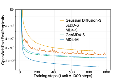
Figure 3: Perplexity on OpenWebText (OWT) validation set during training.

OpenWebText.

We follow Radford et al. [43], Lou et al. [32] to test the language modeling capabilities of our model. Specifically, we train a GPT2-small and GPT2-medium size of MD4 on OpenWebText (98% training, 2% validation) and evaluate zero-shot perplexity unconditionally on the test splits of five benchmark datasets used in Radford et al. [43]: LAMBADA [44], WikiText2, Penn Treebank [45], WikiText103 [46], and One Billion Words [47]. We keep our evaluation setup the same as Lou et al. [32]. To ensure the comparison is fair, we reproduced their result in our implementation.

The results are shown in LABEL:tab:owt-zeroshot-ppl. We can see that our small model outperforms previous best discrete diffusion models on all five tasks. We also confirmed that our re-implementation of SEDD Absorb leads to similar and slightly better results than those reported in their paper. We believe this is because they were using mixed-precision training (thus larger variances) while we are using full precision (float32) training. We are also better than GPT-2 on all tasks except LAMBADA where we are the second best among all methods. When we scale up the model size to medium, we observe that MD4 similarly beats SEDD Absorb and GPT-2 on all tasks except LAMBADA.

Table 1: Zero-shot unconditional perplexity on five benchmark datasets from Radford et al. [43]. The numbers for other methods are from Lou et al. [32] except our reimplementation of SEDD Absorb. Our MD4 model achieves the best result on all benchmarks except LAMBADA where it is the second best. ^∗The GPT-2 numbers are reported for the GPT-2 checkpoint pretrained on WebText instead of OWT thus is not a direct comparison.

Size	Method	LAMBADA	WikiText2	PTB	WikiText103	IBW
Small	GPT-2 (WebText)∗	45.04	42.43	138.43	41.60	75.20
	D3PM	$\leq$ 93.47	$\leq$ 77.28	$\leq$ 200.82	$\leq$ 75.16	$\leq$ 138.92
	Plaid	$\leq$ 57.28	$\leq$ 51.80	$\leq$ 142.60	$\leq$ 50.86	$\leq$ 91.12
	SEDD Absorb	$\leq$ 50.92	$\leq$ 41.84	$\leq$ 114.24	$\leq$ 40.62	$\leq$ 79.29
	SEDD Absorb (reimpl.)	$\leq$ 49.73	$\leq$ 38.94	$\leq$ 107.54	$\leq$ 39.15	$\leq$ 72.96
	MD4 (Ours)	$\leq$ 48.43	$\leq$ 34.94	$\leq$ 102.26	$\leq$ 35.90	$\leq$ 68.10
Medium	GPT-2 (WebText)∗	35.66	31.80	123.14	31.39	55.72
	SEDD Absorb	$\leq$ 42.77	$\leq$ 31.04	$\leq$ 87.12	$\leq$ 29.98	$\leq$ 61.19
	MD4 (Ours)	$\leq$ 44.12	$\leq$ 25.84	$\leq$ 66.07	$\leq$ 25.84	$\leq$ 51.45

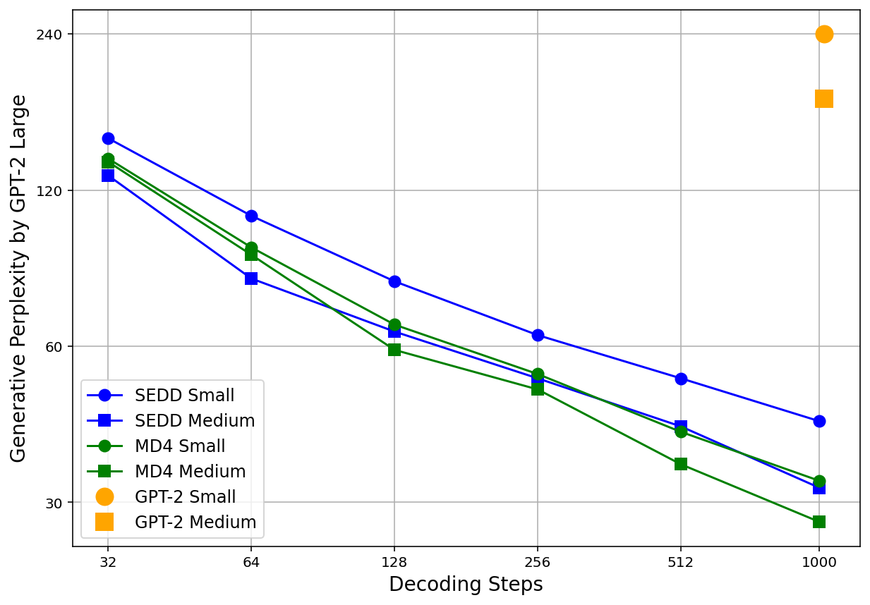
Figure 6: Sample quality evaluated by GPT-2 Large following Lou et al. [32]. We compare MD4 against GPT-2 (auto-regressive baseline) and SEDD (state of the art discrete diffusion model) in generating coherent sequences (1024 tokens). We investigate the effects of two orthogonal factors on sample quality: model size and decoding steps. The numbers for GPT-2 and SEDD are from Lou et al. [32].

To validate that the strong zero-shot performance is a result of a better-trained model, we plot perplexity on the OpenWebText validation set in Figure 3, it demonstrates that our model converges faster and has better final likelihoods than prior methods. We also observed that SEDD [32] has training instabilities. We believe this is due to the score parameterization breaking consistency between forward and reverse processes, as explained in Section 4. Although GenMD4 achieves lower perplexity than MD4, we observed that the learned $w$s can easily overfit to dataset statistics, making it less effective on zero-shot transfer tasks. Beyond likelihood evaluation, we also examine generation quality of our models. Figure 2 showcases a randomly selected, notably coherent sample produced by MD4-medium, alongside its iterative denoising process. Quantitatively, we employ GPT-2 Large model to evaluate perplexity of the generated samples as shown in Figure 6. We can see MD4 is able to outperform its auto-regressive counterpart GPT-2 by a large margin. Sample quality can be improved by two orthogonal strategies: scaling up model size (more compute during training) or increasing decoding steps (more compute during inference). Compared with SEDD, MD4 reaches a new state of the art. Notably, after 64 decoding steps, our MD4 of small size matches the performance of SEDD-medium.

text8.

Following the convention in Austin et al. [14], Lou et al. [32], we experimented with training masked diffusion models on text chunks of length 256. We used the same dataset splits and transformers of the same size to parameterize the backward prediction model. Details can be found in Section H.1. Results are summarized in Table 3. We used the standard bits-per-character metric (a normalized negative log likelihood) for this dataset. We can see that our models outperform previous diffusion models, whether discrete or continuous in nature. We also outperform the best any-order autoregressive models, which do not assume a fixed generation order and has a strong connection to discrete diffusion [48]. Our model is only beaten by an autoregressive transformer and the Discrete Flow (which also used an autoregressive backbone). We believe this is because autoregressive models only require learning a fixed order of generation thus better utilize model capacity.

The text8 dataset has a small vocabulary that consists of 26 letters a-z and a space token. Therefore, we did not expect much flexibility introduced by our state-dependent formulation. Still, with the generalized objective in (14), GenMD4 is able to achieve significantly better BPC than MD4, showing the promise of a state-dependent diffusion on discrete data tasks.

Table 2: Bits Per Character (BPC) on Text8 test set. All models use standard 12-layer transformers similar to GPT2-small [43] except Discrete Flow which uses $8\times 3$ layers.

Method	BPC ($\downarrow$)
Continuous Diffusion
Plaid [22] (Our impl.)	$\leq$ 1.48
BFN [26]	$\leq$ 1.41
Any-order Autoregressive
ARDM [48]	$\leq$ 1.43
MAC [49]	$\leq$ 1.40
Autoregressive
IAF/SCF [50]	1.88
AR Argmax Flow [15]	1.39
Discrete Flow [51]	1.23
Transformer AR [14]	1.23
Discrete Diffusion
Mult. Diffusion [15]	$\leq$ 1.72
D3PM Uniform [14]	$\leq$ 1.61
D3PM Absorb [14]	$\leq$ 1.45
SEDD Absorb [32]	$\leq$ 1.41
MD4 (Ours)	$\leq$ 1.37
GenMD4 (Ours)	$\leq$ 1.34

Table 3: Bits Per Dimension (BPD) on CIFAR-10 test set and Downsampled ImageNet 64$\times$64 [52] validation set. All models in the table are trained without data augmentation.

	Method	#Params	BPD ($\downarrow$)
CIFAR-10	Autoregressive
	PixelRNN [52]		3.00
	Gated PixelCNN [53]		3.03
	PixelCNN++ [54]	53M	2.92
	PixelSNAIL [55]	46M	2.85
	Image Transformer [56]		2.90
	Sparse Transformer [57]	59M	2.80
	Discrete Diffusion
	D3PM Absorb [14]	37M	$\leq$ 4.40
	D3PM Gauss [14]	36M	$\leq$ 3.44
	$\tau$LDR [29]	36M	$\leq$ 3.59
	MD4 (Ours)	28M	$\leq$ 2.78
ImageNet 64$\times$64	Autoregressive
	PixelRNN [52]		3.63
	Gated PixelCNN [53]		3.57
	Sparse Transformer [57]	152M	3.44
	Routing Transformer [58]		3.43
	Perceiver AR [57]	770M	3.40
	Discrete Diffusion
	MD4 (Ours)	198M	$\leq$ 3.42

6.2 Pixel-level image modeling

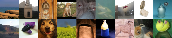
Figure 4: Non cherry-picked unconditional samples from MD4 trained on ImageNet 64x64, treating pixels as discrete tokens. More samples can be found in Figure 5 in Appendix. The model is optimized for likelihood instead of visual quality—see e.g., Kingma et al. [33] for samples from a continuous diffusion model optimized similarly for likelihood.

To demonstrate MD4 beyond text domains, we follow Austin et al. [14], Campbell et al. [29] and train MD4 on order-agnostic image data. Specifically, we take the CIFAR-10 and the Downsampled ImageNet 64$\times$64 [52] datasets and treat each image as a set of discrete tokens from a vocabulary of size $256$ such that the model is unaware of the relative proximity between different pixel values. We compare to other discrete diffusion and autoregressive models that have reported likelihood results on the same dataset, although to our knowledge there are no published result on discrete diffusion methods for ImageNet $64\times 64$ that directly model raw pixel space.

Results are summarized in Table 3. We establish a new state-of-the-art for discrete diffusion models, outperforming previous discrete-time [14] and continuous-time [29] models by a significant margin. Notably, despite lacking knowledge of the ordinal structure of pixel values, MD4 still outperforms models trained with this inductive bias, including D3PM Gauss and $\tau$LDR where the noising distribution is a discrete Gaussian distribution that gives larger probabilities to near pixel values. Our CIFAR-10 model without data augmentation also achieves better likelihood than the previous best autoregressive models on this task, while on ImageNet $64\times 64$ our result is competitive with Transformer AR models of similar sizes, only beaten by Perceiver AR which is approximately $4\times$ larger in model size. We provide a random sample from our ImageNet 64$\times$64 model in Figure 4. More results can be found in in Section H.3.

7 Conclusion

In this work, we revisit masked diffusion models, focusing on a flexible continuous-time formulation. Existing works in this area are not easily accessible to non-specialists and present ELBOs that are difficult to optimize, often resulting in performance that is not competitive with continuous diffusions and autoregressive models. The framework we propose provides a very simple expression of the ELBO as a weighted integral of cross-entropy losses. Additionally, we propose a generalized masked diffusion formulation (GenMD4), where the masking schedule depends on the current state of the process, and derive its corresponding ELBO. Experimentally, on text and image data, the resulting masked diffusions outperform existing discrete and continuous diffusion models and fare very well compared to autoregressive models for most tasks. GenMD4 provides further improvements in terms of likelihoods over the state-independent case.

Although we have improved masked diffusion models, they still suffer from limitations. First, in some tasks such as text8, masked diffusions are not yet competitive with autoregressive models. We conjecture that this is because autoregressive models can better leverage model capacity since they only require learning one order. It would be interesting to develop better architectures for discrete diffusions. Moreover, GenMD4 is promising, but it can easily overfit to the dataset, making it less effective for zero-shot transfer compared to simpler versions. Additionally, inference with a state-dependent schedule is more challenging.

Table 4: Masking schedule formulas.

Masking schedules	$\alpha_{t}$	Cross-entropy loss weight $\frac{\alpha^{\prime}_{t}}{1-\alpha_{t}}$
Linear	$1-t$	$-\frac{1}{t}$
Polynomial	$1-t^{w}$	$-\frac{w}{t}$
Geometric	$\exp\left(-\bar{\beta}_{\text{min}}^{1-t}\bar{\beta}_{\text{max}}^{t}\right)$	$-\frac{\exp\left(-\bar{\beta}_{\text{min}}^{1-t}\bar{\beta}_{\text{max}}^{t}\right)}{1-\exp\left(-\bar{\beta}_{\text{min}}^{1-t}\bar{\beta}_{\text{max}}^{t}\right)}\bar{\beta}_{\text{min}}^{1-t}\bar{\beta}_{\text{max}}^{t}\log\frac{\sigma_{\text{min}}}{\sigma_{\text{max}}}$
Cosine	$1-\cos(\frac{\pi}{2}(1-t))$	$-\frac{\pi}{2}\tan(\frac{\pi}{2}(1-t))$

Appendix A Discrete-time derivation

We divide time from 0 to 1 into $T$ intervals, and let $s(i)=(i-1)/T$, $t(i)=i/T$. The forward transition matrix $Q_{i}\in\mathbb{R}^{(m+1)\times(m+1)}$ ($m$ is vocabulary size) at time $t(i)$ is

$$[Q_{i}]_{jk}=\begin{cases}1&j=k=m\\ 1-\beta_{i}&j=k\neq m\\ \beta_{i}&k=m,j\neq m\\ 0&\text{otherwise}\end{cases}$$

or more compactly written as

$$Q_{i}=(1-\beta_{i})I+\beta_{i}\mathbf{1}e_{m}^{\top},$$

where $\mathbf{1}$ denotes an all-one vector of size $m+1$, and $e_{m}$ is an one-hot vector of size $m+1$ with the $m$-th element (recall that counting starts from $0$) being one. We use an one-hot vector $x_{t}$ of length $m+1$ to denote the discrete state. The forward conditionals are defined as

$$q(x_{t(i)}|x_{s(i)})=\mathrm{Cat}(x_{t(i)};Q_{i}^{\top}x_{s(i)})=x_{s(i)}^{\top}Q_{i}x_{t(i)},$$ (15)

where $Q_{i}^{\top}x_{s(i)}$ is the probabilities for each of the $m+1$ categories that $x_{t(i)}$ can take. The marginal forward distribution at time $t(i)$ given $x_{0}$ is

$$q(x_{t(i)}|x_{0})=\mathrm{Cat}(x_{t(i)};\bar{Q}_{i}^{\top}x_{0})=x_{0}^{\top}\bar{Q}_{i}x_{t(i)},$$

where $\bar{Q}_{i}=\prod_{j=1}^{i}Q_{j}=\prod_{j=1}^{i}(1-\beta_{j})I+\big{(}1-\prod_{j=1}^{i}(1-\beta_{j})\big{)}\mathbf{1}e_{m}^{\top}$. To see what this leads to in continuous time, we let $\beta_{i}=\frac{\beta(t(i))}{T}$ and $T\to\infty$:

$$\prod_{j=1}^{i}(1-\beta_{j}) =\exp\Big{(}\sum_{j=1}^{i}\log(1-\beta_{j})\Big{)}$$

$$=\exp\Big{(}\sum_{j=1}^{i}-\frac{\beta(t(j))}{T}+o(1/T)\Big{)}$$

$$\overset{T\to\infty}{\to}\exp\Big{(}-\int_{0}^{t(i)}\beta(s)\mathrm{d}s\Big{)}.$$

We let $\bar{Q}(t)$ denote the limit of $\bar{Q}_{i}$ in this case:

$$\bar{Q}(t) =\exp\big{(}-\int_{0}^{t}\beta(s)\mathrm{d}s\big{)}I+\Big{(}1-\exp\big{(}-\int_{0}^{t}\beta(s)\mathrm{d}s\big{)}\Big{)}\mathbf{1}e_{m}^{\top}$$

$$\triangleq\alpha_{t}I+(1-\alpha_{t})\mathbf{1}e_{m}^{\top}.$$

Here we define $\alpha_{t}\triangleq\exp(-\int_{0}^{t}\beta(s)\mathrm{d}s)$. And the marginal forward transition is

$$q(x_{t}|x_{0})=\mathrm{Cat}(x_{t};\bar{Q}(t)^{\top}x_{0})=x_{0}^{\top}\bar{Q}(t)x_{t}=\alpha_{t}x_{0}^{\top}x_{t}+(1-\alpha_{t})e_{m}^{\top}x_{t}.$$ (16)

Appendix B Continuous-time derivation

We consider a continuous-time Markov chain with transition rates

$$Q(t)=(Q_{i}-I)/(1/T)=\beta(t)(\mathbf{1}e_{m}^{\top}-I).$$ (17)

For simplicity, we let $Q=\mathbf{1}e_{m}^{\top}-I$. The marginal forward distribution at time $t$ given $x_{0}$ is $q(x_{t}|x_{0})=\mathrm{Cat}(x_{t};\bar{Q}(t)^{\top}x_{0})$, where

$$\bar{Q}(t)=\exp\Big{(}\int_{0}^{t}Q(s)\mathrm{d}s\Big{)}=\exp\Big{(}Q\int_{0}^{t}\beta(s)\mathrm{d}s\Big{)}=\exp(\bar{\beta}(t)Q).$$

Here we define $\bar{\beta}(t)\triangleq\int_{0}^{t}\beta(s)\mathrm{d}s$. The matrix exponential can be computed via eigendecomposition:

$$\bar{\beta}(t)Q=U\Lambda U^{-1},$$

where

$$U =I-e_{m}e_{m}^{\top}+\frac{1}{\sqrt{n+1}}\mathbf{1}e_{m}^{\top},$$

$$U^{-1} =I+\sqrt{n+1}e_{m}e_{m}^{\top}-\mathbf{1}e_{m}^{\top},$$

$$\Lambda =\bar{\beta}(t)(e_{m}e_{m}^{\top}-I),$$

and thus $\exp(\Lambda)=\alpha_{t}I+(1-\alpha_{t})e_{m}e_{m}^{\top}$,

$$\bar{Q}(t)=U\exp(\Lambda)U^{-1}=\alpha_{t}I+(1-\alpha_{t})\mathbf{1}e_{m}^{\top}.$$

A simpler derivation uses the following property:

$$Q^{2}=-Q.$$

Therefore,

$$\bar{Q}(t) =\exp(\bar{\beta}(t)Q)$$

$$=I+\bar{\beta}(t)Q+\frac{1}{2}\bar{\beta}(t)^{2}Q^{2}+\frac{1}{3}\bar{\beta}(t)^{3}Q^{3}+\dots$$

$$=I+Q-(1-\bar{\beta}(t)+\frac{1}{2}\bar{\beta}(t)^{2}-\frac{1}{3}\bar{\beta}(t)^{3}+\dots)Q$$

$$=I+Q-\exp(-\bar{\beta}(t))Q$$

$$=\alpha_{t}I+(1-\alpha_{t})\mathbf{1}e_{m}^{\top}.$$

This marginal forward transition matrix at time $t$ coincides with the result (1) we get by taking the limit of discrete-time derivation.

Arbitrary discretization of the continuous-time forward process.

For the discrete-time process we have defined the per-step transition in (15). For the continuous-time process, we can derive the transition matrix $\bar{Q}(s,t)_{ij}\triangleq q(x_{t}=j|x_{s}=i)$ between two arbitrary time $s$ and $t$ as the solution to the following differential equation (known as Kolmogorov forward equation)

$$\frac{\mathrm{d}}{\mathrm{d}t}\bar{Q}(s,t) =\bar{Q}(s,t)Q(t)\text{ where }Q(t)=\beta(t)Q$$

with initial condition $\bar{Q}(s,s)=I$. The solution is given by

$$\bar{Q}(s,t)=\exp\big{(}(\bar{\beta}(t)-\bar{\beta}(s))Q\big{)}=\bar{Q}(s)^{-1}\bar{Q}(t).$$

Routine work (using the Woodbury matrix inversion lemma) shows that

$$\bar{Q}(t)^{-1}=\alpha_{t}^{-1}I+(1-\alpha_{t}^{-1})\mathbf{1}e_{m}^{\top}.$$

Plugging the result back, we get the forward transition distribution from $s$ to $t$:

$$q(x_{t}|x_{s}) =\mathrm{Cat}(x_{t};\bar{Q}(s,t)^{\top}x_{s})=x_{s}^{\top}\bar{Q}(s,t)x_{t},$$ (18)

$$\text{ where }\bar{Q}(s,t) \triangleq\bar{Q}(s)^{-1}\bar{Q}(t)=\frac{\alpha_{t}}{\alpha_{s}}I+\big{(}1-\frac{\alpha_{t}}{\alpha_{s}}\big{)}\mathbf{1}e_{m}^{\top}.$$

Appendix C Time reversal of the forward process given $x_{0}$

The analytic property of our forward process allows to compute many quantities of interest in closed form. One such quantity frequently used in diffusion models is the time reversal of the forward process given $x_{0}$: $q(x_{s}|x_{t},x_{0})$. We can compute it using (16) and (18) as

$$q(x_{s}|x_{t},x_{0}) =\frac{q(x_{t}|x_{s})q(x_{s}|x_{0})}{q(x_{t}|x_{0})}$$

$$=\begin{cases}\frac{\alpha_{s}-\alpha_{t}}{1-\alpha_{t}}x_{s}^{\top}x_{0}&x_{s}\neq m,x_{t}=m\\ \frac{1-\alpha_{s}}{1-\alpha_{t}}&x_{s}=m,x_{t}=m\\ x_{s}^{\top}x_{t}&x_{t}\neq m.\end{cases}$$ (19)

We can rewrite the above using reverse transition matrix $\bar{R}^{x_{0}}(t,s)\in\mathbb{R}^{(m+1)\times(m+1)}$ as

$$q(x_{s}|x_{t},x_{0})=\mathrm{Cat}(x_{s};\bar{R}^{x_{0}}(t,s)^{\top}x_{t}),\text{ where }\bar{R}^{x_{0}}(t,s)=I+\frac{\alpha_{s}-\alpha_{t}}{1-\alpha_{t}}e_{m}(x_{0}-e_{m})^{\top}.$$

We are also interested in what would happen in the infinitesimal time limit, i.e., when $s=t-\Delta t$ and $\Delta t\to 0$. Note that $\frac{\mathrm{d}\alpha_{t}}{\mathrm{d}t}=-\beta(t)\alpha_{t}$,

$$\alpha_{t-\Delta t}-\alpha_{t}=\alpha_{t}^{\prime}\Delta t+o(\Delta t).$$

Plugging it into the original formula, we get

$$\bar{R}^{x_{0}}(t,t-\Delta t)=I+\frac{\alpha_{t}^{\prime}}{1-\alpha_{t}}e_{m}(x_{0}-e_{m})^{\top}\Delta t+o(\Delta t).$$

Comparing the above with the transition rate matrix $R^{x_{0}}(t)$ definition

$$\bar{R}^{x_{0}}(t,t-\Delta t)=I+R^{x_{0}}(t)\Delta t+o(\Delta t),$$

we have determined the transition rate matrix for the reverse process conditioned on $x_{0}$:

$$R^{x_{0}}(t) =\frac{\alpha_{t}^{\prime}}{1-\alpha_{t}}e_{m}(x_{0}-e_{m})^{\top}.$$ (20)

Appendix D Details of the ELBO

Using (C) and (3), we compute the KL divergences between forward and backward transitions

$$\mathrm{KL}({q(x_{s}|x_{t},x_{0})}\|{p_{\theta}(x_{s}|x_{t})}) =\mathrm{KL}({q(x_{s}|x_{t},x_{0})}\|{q(x_{s}|x_{t},\mu_{\theta}(x_{t},t))})$$ (21)

$$=\begin{cases}\sum_{x_{s}=0}^{m}q(x_{s}|x_{t},x_{0})\log\frac{q(x_{s}|x_{t},x_{0})}{q(x_{s}|x_{t},\mu_{\theta}(x_{t},t))}&x_{t}=m\\ 0&x_{t}\neq m\end{cases}$$

$$=\delta_{x_{t}=m}\sum_{k\neq m}\frac{\alpha_{s}-\alpha_{t}}{1-\alpha_{t}}x_{0}^{\top}e_{k}\log\frac{x_{0}^{\top}e_{k}}{\mu_{\theta}(x_{t},t)^{\top}e_{k}}$$

$$=-\delta_{x_{t}=m}\frac{\alpha_{s}-\alpha_{t}}{1-\alpha_{t}}x_{0}^{\top}\log\mu_{\theta}(x_{t},t).$$

Note that $0\log 0=0$. In this case, the reconstruction term becomes

$$\mathbb{E}_{q(x_{t(1)}|x_{0})}[\log p(x_{0}|x_{t(1)})] =\sum_{k=0}^{m}q_{t(1)|0}(k|x_{0})\log\frac{q_{t(1)|0}(k|x_{0})}{\sum_{j\neq m}q_{t(1)|0}(k|j)}$$

$$=\alpha_{t(1)}\cdot\log\frac{\alpha_{t(1)}}{\alpha_{t(1)}}+(1-\alpha_{t(1)})\log\frac{1}{m}$$

$$=-(1-\alpha_{t(1)})\log m.$$

The prior KL term can be computed as

$$\mathrm{KL}({q(x_{1}|x_{0})}\|{p(x_{1})})=\mathrm{KL}({\delta_{x_{1},m}}\|{\delta_{x_{1},m}})=0.$$

As usual, we take the continuous-time limit by letting $T\to\infty$:

$$\mathcal{L}_{\infty} \triangleq\lim_{T\to\infty}\mathcal{L}_{T}$$

$$=\lim_{T\to\infty}\sum_{i=2}^{T}-\frac{\alpha_{s(i)}-\alpha_{t(i)}}{s(i)-t(i)}\frac{s(i)-t(i)}{1-\alpha_{t(i)}}x_{0}^{\top}\mathbb{E}_{q(x_{t(i)}|x_{0})}\left[\delta_{x_{t(i)},m}\log\mu_{\theta}(x_{t(i)},t(i))\right]$$

$$=\int_{t(1)}^{1}\frac{\alpha_{t}^{\prime}}{1-\alpha_{t}}x_{0}^{\top}\mathbb{E}_{q(x_{t}|x_{0})}\left[\delta_{x_{t},m}\log\mu_{\theta}(x_{t},t)\right]\mathrm{d}t.$$

Appendix E Avoiding undefined KL divergence

When defining the forward process, we often do not want $\alpha_{1}$ to be exactly 0, or equivalently, $\lambda_{1}$ to be $\infty$ for numerical stability reasons. Instead, we set $\lambda_{1}$ to be a finite value, and thereby $\alpha_{1}$ has a small positive value. This has a problem that the support of $q(x_{1}|x_{0})$ is no longer $\{m\}$ and instead becomes $\{m,x_{0}\}$. As a result, the KL divergence between $q(x_{1}|x_{0})$ and $p(x_{1})$ is undefined because $q(x_{1}|x_{0})$ is not absolutely continuous with respect to $p(x_{1})=\delta_{x_{1},m}$. To resolve the issue, we modify the prior distribution $p(x_{1})$ such that it has support over all $m+1$ values. One such choice is letting

$$p(x_{1})=\frac{\alpha_{1}}{m}\sum_{j\neq m}\delta_{x_{1},j}+(1-\alpha_{1})\delta_{x_{1},m}.$$

Then, the prior KL divergence term becomes

$$\mathrm{KL}({q(x_{1}|x_{0})}\|{p(x_{1})}) =\sum_{x_{1}=0}^{m}q(x_{1}|x_{0})\log\frac{q(x_{1}|x_{0})}{p(x_{1})}$$

$$=\sum_{x_{1}=0}^{m}(\alpha_{1}\delta_{x_{1},x_{0}}+(1-\alpha_{1})\delta_{x_{1},m})\log\frac{\alpha_{1}\delta_{x_{1},x_{0}}+(1-\alpha_{1})\delta_{x_{1}=m}}{p(x_{1})}$$

$$=\alpha_{1}\log\frac{\alpha_{1}}{\alpha_{1}/m}+(1-\alpha_{1})\log\frac{1-\alpha_{1}}{1-\alpha_{1}}$$

$$=\alpha_{1}\log m.$$

Appendix F Unifying Existing Masked Diffusion Models

F.1 The CTMC point of view

We first prove a lemma that connects the forward and reverse transition rate matrices. This follows from the results in [29] but we give a proof for completeness.

Lemma 2.

The forward transition rate matrix $Q(t)$ and the reverse transition rate matrix (given $x_{0}$) $R^{x_{0}}(t)$ satisfy:

$$R^{x_{0}}(t)_{kj}=Q(t)_{jk}\frac{q_{t|0}(j|x_{0})}{q_{t|0}(k|x_{0})}\text{ for }j\neq k.$$ (22)

Proof    Consider the backward transition from time $t+\tau$ to $t$. For $j\neq k$, Bayes’ rule yields

$$q(x_{t}=j|x_{t+\tau}=k,x_{0}) =\frac{q(x_{t}=j|x_{0})q(x_{t+\tau}=k|x_{t}=j)}{q(x_{t+\tau}=k|x_{0})}$$

$$=\frac{q(x_{t}=j|x_{0})(\delta_{jk}+Q(t)_{jk}\tau+o(\tau))}{q(x_{t+\tau}=k|x_{0})}$$

$$\overset{\tau\to 0}{=}\delta_{kj}+\frac{q(x_{t}=j|x_{0})}{q(x_{t}=k|x_{0})}Q(t)_{jk}\tau+o(\tau).$$

Then, it follows from the definition of the transition rate matrix that $R^{x_{0}}(t)_{kj}=Q(t)_{jk}\frac{q_{t|0}(j|x_{0})}{q_{t|0}(k|x_{0})}$. ∎

Proposition 3.

We use the shorthand $R_{\theta}(t)_{kj}$ to denote the approximate backward transition rate from the state $k$ to $j$ obtained by substituting our prediction model $\mu_{\theta}(k)$ for $x_{0}$ in $R^{x_{0}}(t)_{kj}$. Then, the continuous-time objective (4) can be equivalently expressed as

$$\mathcal{L}_{\infty}=-\int_{t(1)}^{1}\mathbb{E}_{q_{t|0}(k|x_{0})}\Big{[}R_{\theta}(t)_{kk}+\sum_{j\neq k}Q(t)_{kj}\log R_{\theta}(t)_{jk}\Big{]}\mathrm{d}t+\text{C},$$ (23)

where $C$ is a constant independent of $\theta$.

Proof   To rewrite our objective $\mathcal{L}_{\infty}$ with the transition rate matrices, we first go back to (21). There, instead of plugging in the explicit form of $\bar{R}^{x_{0}}(t,s)$, we substitute it with (7) which leverages the transition rate $R^{x_{0}}(t)$. To simplify the notation, we assume $x_{t}=k$ and use the shorthand $R_{\theta}(t)_{kj}\triangleq R^{\mu_{\theta}(k)}(t)_{kj}$. We then have

$$\mathrm{KL}({q(x_{t-\Delta t}|x_{t},x_{0})}\|{p_{\theta}(x_{t-\Delta t}|x_{t})})$$

$$=\mathrm{KL}({\mathrm{Cat}(x_{s};\bar{R}^{x_{0}}(t,t-\Delta t)^{\top}e_{k})}\|{\mathrm{Cat}(x_{s};\bar{R}^{\mu_{\theta}(k)}(t,t-\Delta t)^{\top}e_{k})})$$

$$=\sum_{j=0}^{m}e_{k}^{\top}(I+R^{x_{0}}(t)\Delta t+o(\Delta t))e_{j}\log\frac{e_{k}^{\top}(I+R^{x_{0}}(t)\Delta t+o(\Delta t))e_{j}}{e_{k}^{\top}(I+R_{\theta}(t)\Delta t+o(\Delta t))e_{j}}$$

$$=(1+R^{x_{0}}(t)_{kk}\Delta t)\log\frac{1+R^{x_{0}}(t)_{kk}\Delta t+o(\Delta t)}{1+R_{\theta}(t)_{kk}\Delta t+o(\Delta t)}$$

$$\quad+\sum_{j\neq k}(R^{x_{0}}(t)_{kj}\Delta t)\log\frac{R^{x_{0}}(t)_{kj}\Delta t+o(\Delta t)}{R_{\theta}(t)_{kj}\Delta t+o(\Delta t)}+o(\Delta t)$$

$$=(R^{x_{0}}(t)_{kk}-R_{\theta}(t)_{kk})\Delta t+\sum_{j\neq k}(R^{x_{0}}(t)_{kj}\Delta t)\log\frac{R^{x_{0}}(t)_{kj}\Delta t+o(\Delta t)}{R_{\theta}(t)_{kj}\Delta t+o(\Delta t)}+o(\Delta t).$$

For the last identity, we have used the fact that $\log(1+x)=x+o(x)$. To obtain $\mathcal{L}_{\infty}$, we take the limit of $\mathcal{L}_{T}$ as $T\to\infty$, which is equivalent to letting $\Delta t=1/T\to 0$. We obtain

$$\mathcal{L}_{\infty} =\lim_{T\to\infty}\sum_{i=2}^{T}\mathbb{E}_{q(x_{t(i)}|x_{0})}[\mathrm{KL}({q(x_{s(i)}|x_{t(i)},x_{0})}\|{p_{\theta}(x_{s(i)}|x_{t(i)})})]$$

$$=\lim_{T\to\infty}\sum_{i=2}^{T}\mathbb{E}_{q(x_{t(i)}|x_{0})}\Big{[}\Big{(}R^{x_{0}}(t(i))_{kk}-R_{\theta}(t(i))_{kk}$$

$$\quad+\sum_{j\neq k}R^{x_{0}}(t(i))_{kj}\log\frac{R^{x_{0}}(t(i))_{kj}\Delta t+o(\Delta t)}{R_{\theta}(t(i))_{kj}\Delta t+o(\Delta t)}\Big{)}\Delta t+o(\Delta t)\Big{]}$$

$$=\int_{t(1)}^{1}\mathbb{E}_{q_{t|0}(k|x_{0})}\Big{[}R^{x_{0}}(t)_{kk}-R_{\theta}(t)_{kk}+\sum_{j\neq k}R^{x_{0}}(t)_{kj}\log\frac{R^{x_{0}}(t)_{kj}}{R_{\theta}(t)_{kj}}\Big{]}\mathrm{d}t.$$

Note that $R^{x_{0}}(t)$ is a constant matrix independent of $\theta$. Absorbing all constant terms into $C$, we have

$$\mathcal{L}_{\infty}=-\int_{t(1)}^{1}\mathbb{E}_{q_{t|0}(k|x_{0})}\Big{[}R_{\theta}(t)_{kk}+\sum_{j\neq k}R^{x_{0}}(t)_{kj}\log R_{\theta}(t)_{kj}\Big{]}\mathrm{d}t+C.$$

Next, we subtitute $R^{x_{0}}(t)$ with the forward transition rate using Lemma 2:

$$\mathcal{L}_{\infty} =-\int_{t(1)}^{1}\mathbb{E}_{q_{t|0}(k|x_{0})}\Big{[}R_{\theta}(t)_{kk}+\sum_{j\neq k}Q(t)_{jk}\frac{q_{t|0}(j|x_{0})}{q_{t|0}(k|x_{0})}\log R_{\theta}(t)_{kj}\Big{]}\mathrm{d}t+C$$

$$=-\int_{t(1)}^{1}\Big{[}\sum_{k=0}^{m}q_{t|0}(k|x_{0})R_{\theta}(t)_{kk}+\sum_{k=0}^{m}\sum_{j\neq k}Q(t)_{jk}q_{t|0}(j|x_{0})\log R_{\theta}(t)_{kj}\Big{]}\mathrm{d}t+C$$

$$=-\int_{t(1)}^{1}\Big{[}\sum_{k=0}^{m}q_{t|0}(k|x_{0})R_{\theta}(t)_{kk}+\sum_{k=0}^{m}\sum_{j\neq k}Q(t)_{kj}q_{t|0}(k|x_{0})\log R_{\theta}(t)_{jk}\Big{]}\mathrm{d}t+C,$$

where the last identity used the discrete analog to integration-by-part (or summation-by-part): $\sum_{k=0}\sum_{j\neq k}f(j,k)=\sum_{k=0}\sum_{j\neq k}f(k,j)$. Rearranging the terms then gives (23).

∎

F.2 Differences from Campbell et al. [29]

Campbell et al. [29] used the first term of (8) as the training loss. A key limitation of this loss function is from the inner summation term

$$\sum_{j\neq k}Q(t)_{kj}\log R_{\theta}(t)_{jk}.$$

Recall that $R_{\theta}(t)_{jk}$ is computed as substituting our neural network prediction model $\mu_{\theta}(j)$ for $x_{0}$ in $R^{x_{0}}(t)_{jk}$. Therefore, the summation together with $R_{\theta}(t)_{kk}$ requires $m$ evaluations of $\mu_{\theta}(\cdot)$. This is prohibitive since the neural network model is usually expensive. To resolve this issue, Campbell et al. [29] proposed to rewrite the sum as

$$\mathbb{E}_{j\sim\tilde{q}(\cdot|k)}\left[Z_{k}\log R_{\theta}(t)_{jk}\right]\text{\quad where\quad}\tilde{q}(j|k)=\frac{Q(t)_{kj}}{Z_{k}},Z_{k}\triangleq\sum_{j^{\prime}\neq k}Q(t)_{kj^{\prime}}$$

and estimate it through Monte Carlo. Taking into account the outer expectation under $q_{t|0}(k|x_{0})$, the computation of the loss then becomes a doubly stochastic estimate (using $k\sim q_{t|0}(k|x_{0})$ and $j\sim\tilde{q}(j|k)$) which suffers from large variance. In contrast, the form of our loss (4) only requires evaluating $\mu_{\theta}$ once for a single stochastic estimation of the expectation w.r.t. $q(x_{t}|x_{0})$.

F.3 Score parameterization

We provide a simpler derivation of the score-based loss [35, 32] below. We start from the form of the ELBO in (23) and rewrite it as

$$\mathcal{L}_{\infty} =\int_{t(1)}^{1}\mathbb{E}_{q_{t|0}(k|x_{0})}\Big{[}\sum_{j\neq k}\Big{(}R^{\mu_{\theta}}(t)_{kj}-R^{x_{0}}(t)_{kj}+R^{x_{0}}(t)_{kj}\log\frac{R^{x_{0}}(t)_{kj}}{R^{\mu_{\theta}}(t)_{kj}}\Big{)}\Big{]}\mathrm{d}t.$$ (24)

For the last identity we used the zero-row-sum property of transition rate matrix:

$$R^{x_{0}}(t)_{kk}=-\sum_{j\neq k}R^{x_{0}}(t)_{kj}.$$

If we plug (22) into (24) and reparameterize with a score model

$$s_{\theta}(x_{t})_{j}\triangleq\frac{q_{t|0}(j|\mu_{\theta}(x_{t}))}{q(x_{t}|\mu_{\theta}(x_{t}))},$$ (25)

we recover the score entropy loss function from Benton et al. [35], Lou et al. [32]:

$$\mathcal{L}_{\infty}=\int_{t(1)}^{1}\mathbb{E}_{q_{t|0}(k|x_{0})}\Big{[}\sum_{j\neq k}Q(t)_{jk}\Big{(}s_{\theta}(k)_{j}-\frac{q_{t|0}(j|x_{0})}{q_{t|0}(k|x_{0})}\log s_{\theta}(k)_{j}+\psi\Big{(}\frac{q_{t|0}(j|x_{0})}{q_{t|0}(k|x_{0})}\Big{)}\Big{)}\Big{]}\mathrm{d}t,$$

where $\psi(y)\triangleq y\log y-y$. Note that our derivation above is different and simpler than that of Campbell et al. [29] (which Lou et al. [32] is based on) since we leverage the conditional reverse transition rate given $x_{0}$ instead of the transition rate matrix of the reverse process. We can further simplify the loss with the following relationship between the conditional score and $x_{0}$:

$$\frac{q_{t|0}(j|x_{0})}{q_{t|0}(k|x_{0})}=\frac{x_{0}^{\top}\bar{Q}(t)e_{j}}{x_{0}^{\top}\bar{Q}(t)e_{k}}=\frac{\alpha_{t}}{1-\alpha_{t}}x_{0}^{\top}e_{j} \text{ for }k=m,j\neq k.$$ (26)

Note that only the result under the case $k=m$ is needed. This is because when $x_{t}$ is unmasked, at any time between $0$ and $t$, the state must stay unchanged and remain $x_{0}$. As a result, $\mathrm{KL}({q(x_{t-\Delta t}|x_{t},x_{0})}\|{p_{\theta}(x_{t-\Delta t}|x_{t})})=0$ for $x_{t}\neq m$. From (17), we know $Q(t)_{jk}=\beta(t)(\delta_{mk}-\delta_{jk})$. Combining (26) and (9), we get

$$\mathcal{L}_{\infty}=\int_{t(1)}^{1}\beta(t)\Big{(}\mathbb{E}_{q_{t|0}(k|x_{0})}\big{[}\delta_{mk}\big{(}\sum_{j\neq k}s_{\theta}(k)_{j}-\frac{\alpha_{t}}{1-\alpha_{t}}x_{0}^{\top}\log s_{\theta}(k)\big{)}\big{]}+\psi\big{(}\frac{\alpha_{t}}{1-\alpha_{t}}\big{)}\Big{)}\mathrm{d}t.$$ (27)

Further, we can show the connection between (27) and (4) by reverting the score parameterization to a mean parameterization using (25), or equivalently $s_{\theta}(x_{t})_{j}=\frac{\alpha_{t}}{1-\alpha_{t}}\mu_{\theta}(x_{t})^{\top}e_{j}$. By doing so, we obtain

$$\mathcal{L}_{\infty}=\int_{t(1)}^{1}\beta(t)\Big{(}\mathbb{E}_{q_{t|0}(k|x_{0})}\big{[}\delta_{mk}\big{(}\sum_{j\neq k}s_{\theta}(k)_{j}-\frac{\alpha_{t}}{1-\alpha_{t}}x_{0}^{\top}\log\mu_{\theta}(k)\big{]}+\frac{\alpha_{t}}{1-\alpha_{t}}\big{)}\mathrm{d}t.$$

Observing that

$$\sum_{j\neq m}s_{\theta}(m)_{j}=\frac{\alpha_{t}}{1-\alpha_{t}},$$ (28)

we conclude that this recovers the objective in (4). Interestingly, in Lou et al. [32] the score parameterization is not constrained to satisfy (28). That means the learned backward model might be incompatible with the forward process.

It is easy to prove Proposition 1 from Equation 26.

Proof of Proposition 1

$$\frac{q_{t}(j)}{q_{t}(m)} =\frac{\sum_{x_{0}}q_{t|0}(j|x_{0})q(x_{0})}{q_{t}(m)}=\frac{\sum_{x_{0}}q_{t|0}(j|x_{0})q_{0|t}(x_{0}|m)}{q_{t|0}(m|x_{0})}=\mathbb{E}_{x_{0}|x_{t}=m}\left[\frac{q_{t|0}(j|x_{0})}{q_{t|0}(m|x_{0})}\right]$$

$$=\mathbb{E}_{x_{0}|x_{t}=m}\left[\frac{\alpha_{t}}{1-\alpha_{t}}x_{0}^{\top}e_{j}\right]=\frac{\alpha_{t}}{1-\alpha_{t}}\mathbb{E}[x_{0}|x_{t}=m]^{\top}e_{j}.$$

∎

F.4 Differences from Sundae

Sundae [59, 60] uses a linear noise schedule and uniformly corrupts data with random tokens in the vocab (Uniform style). Additionally it uses a second loss term from cross entropy between un-corrupted data and 1-step unrolled model prediction. Similar ideas have been proposed in [61].

Appendix G Details for state-dependent rates

G.1 Derivations and time continuous limit

All derivations in this section assume that $x_{t}$ is a single token, while for $N$ tokens the masked diffusion with state-dependent rates factorises across the $N$ tokens. Learning from data of $N$ tokens using variational inference is discussed in Section G.2.

Given the forward transition $q(x_{t}|x_{s})$ and marginal $q(x_{s}|x_{0})$ derived in main text (Section 5) The reversal given $x_{0}$ is $q(x_{s}|x_{t},x_{0})=\mathrm{Cat}(x_{s};\bar{R}^{x_{0}}(t,s)^{\top}x_{t})$ for

$$\bar{R}^{x_{0}}(t,s)_{jk}=\begin{cases}\big{(}\frac{\alpha_{s}-\alpha_{t}}{\mathbf{1}-\alpha_{t}}\big{)}^{\top}x_{0}x_{0}^{\top}e_{k}&j=m,k\neq m\\ \big{(}\frac{\mathbf{1}-\alpha_{s}}{\mathbf{1}-\alpha_{t}}\big{)}^{\top}x_{0}&j=m,k=m\\ \delta_{jk}&j\neq m.\end{cases}$$

or alternatively can be written as

$$q(x_{s}|x_{t},x_{0}) =\frac{q(x_{t}|x_{s})q(x_{s}|x_{0})}{q(x_{t}|x_{0})}$$

$$=\frac{\left[\frac{\alpha_{t}^{\top}x_{s}}{\alpha_{s}^{\top}x_{s}}x_{s}^{\top}x_{t}+(1-\frac{\alpha_{t}^{\top}x_{s}}{\alpha_{s}^{\top}x_{s}})e_{m}^{\top}x_{t}\right]\left[\alpha_{s}^{\top}x_{0}x_{0}^{\top}x_{s}+(1-\alpha_{s}^{\top}x_{0})e_{m}^{\top}x_{s}\right]}{\left[\alpha_{t}^{\top}x_{0}x_{0}^{\top}x_{t}+(1-\alpha_{t}^{\top}x_{0})e_{m}^{\top}x_{t}\right]}.$$ (29)

To simplify this expression we consider the two cases: either $x_{t}=m$ (i.e. $x_{t}$ is mask) or $x_{t}\neq m$ where in the second case $x_{t}=x_{0}$. For the case $x_{t}=m$, the denominator in (29) simplifies as

$$q(x_{t}=m|x_{0})=1-\alpha_{t}^{\top}x_{0}$$

due to $x_{0}^{\top}x_{t}=0$ since $x_{0}\neq m$, i.e. the observed token $x_{0}$ cannot be a mask. Then given that $x_{t}=m$ the probability that $x_{s}=x_{t}=m$ is

$$\frac{1-\alpha_{s}^{\top}x_{0}}{1-\alpha_{t}^{\top}x_{0}}=\frac{({\bf 1}-\alpha_{s})^{\top}x_{0}}{({\bf 1}-\alpha_{t})^{\top}x_{0}}=\left(\frac{{\bf 1}-\alpha_{s}}{{\bf 1}-\alpha_{t}}\right)^{\top}x_{0}$$ (30)

while the remaining probability for $x_{s}=x_{0}\neq m$ is

$$\frac{(\alpha_{s}-\alpha_{t})^{\top}x_{0}}{1-\alpha_{t}^{\top}x_{0}}=\frac{(\alpha_{s}-\alpha_{t})^{\top}x_{0}}{({\bf 1}-\alpha_{t})^{\top}x_{0}}=\left(\frac{\alpha_{s}-\alpha_{t}}{{\bf 1}-\alpha_{t}}\right)^{\top}x_{0}.$$ (31)

Then, combining (30) and (31) to write $q(x_{s}|x_{t}=m,x_{0})$ in an unified way yields the expression (13) in the main Section 5. In the second case, when $x_{t}=x_{0}\neq m$, $q(x_{s}|x_{t}\neq m,x_{0})$ from (29) simplifies dramatically and it becomes $q(x_{s}|x_{t}\neq m,x_{0})=x_{t}^{\top}x_{s}$ which is a point mass that sets $x_{s}=x_{t}$.

Derivation of the continuous-time limit of the loss in (14).

To simplify the notation, we let $\xi_{s,t}\triangleq\frac{\alpha_{s}-\alpha_{t}}{1-\alpha_{t}}$. We first compute the KL divergence terms in the discrete-time ELBO as

$$\mathrm{KL}({q(x_{s}|x_{t},x_{0})}\|{p_{\theta}(x_{s}|x_{t})})$$

$$=\begin{cases}\sum_{x_{s}=0}^{m}q(x_{s}|x_{t},x_{0})\log\frac{q(x_{s}|x_{t},x_{0})}{p_{\theta}(x_{s}|x_{t})}&x_{t}=m\\ 0&x_{t}\neq m\end{cases}$$

$$=\delta_{x_{t},m}\Big{[}\sum_{k\neq m}\xi_{s,t}^{\top}x_{0}x_{0}^{\top}e_{k}\log\frac{\xi_{s,t}^{\top}x_{0}x_{0}^{\top}e_{k}}{\xi_{s,t}^{\top}\mathrm{diag}(\mu_{\theta}(x_{t},t))e_{k}}+(1-\xi_{s,t})^{\top}x_{0}\log\frac{(1-\xi_{s,t})^{\top}x_{0}}{(1-\xi_{s,t})^{\top}\mu_{\theta}(x_{t},t)}\Big{]}$$

$$=\delta_{x_{t},m}\Big{[}-\xi_{s,t}^{\top}x_{0}x_{0}^{\top}\log\mu_{\theta}(x_{t},t)+(1-\xi_{s,t})^{\top}x_{0}\log\frac{(1-\xi_{s,t})^{\top}x_{0}}{(1-\xi_{s,t})^{\top}\mu_{\theta}(x_{t},t)}\Big{]}.$$

Let $\Delta_{t}\triangleq\frac{1}{T}=t(i)-s(i)$ for all $i$. Plugging $\alpha_{t-\Delta t}=\alpha_{t}-\alpha_{t}^{\prime}\Delta t+o(\Delta t)$ into the above formula and letting $\gamma_{t}=\frac{\alpha_{t}^{\prime}}{1-\alpha_{t}}$, we get

$$\mathrm{KL}({q(x_{s}|x_{t},x_{0})}\|{p_{\theta}(x_{s}|x_{t})})$$

$$=\delta_{x_{t},m}\left[\gamma_{t}^{\top}x_{0}x_{0}^{\top}\log\mu_{\theta}(x_{t},t)\Delta t+\left(1+\gamma_{t}^{\top}x_{0}\Delta t\right)\cdot\log\frac{1+\gamma_{t}^{\top}x_{0}\Delta t+o(\Delta t)}{1+\gamma_{t}^{\top}\mu_{\theta}(x_{t},t)\Delta t+o(\Delta t)}+o(\Delta t)\right]$$

$$=\delta_{x_{t},m}\left[\gamma_{t}^{\top}x_{0}x_{0}^{\top}\log\mu_{\theta}(x_{t},t)\Delta t+\left(1+\gamma_{t}^{\top}x_{0}\Delta t\right)\left(\gamma_{t}^{\top}x_{0}\Delta t-\gamma_{t}^{\top}\mu_{\theta}(x_{t},t)\Delta t+o(\Delta t)\right)+o(\Delta t)\right]$$

$$=\delta_{x_{t},m}\left[\gamma_{t}^{\top}x_{0}x_{0}^{\top}\log\mu_{\theta}(x_{t},t)\Delta t+\gamma_{t}^{\top}x_{0}\Delta t-\gamma_{t}^{\top}\mu_{\theta}(x_{t},t)\Delta t+o(\Delta t)\right]$$

$$=\delta_{x_{t},m}\cdot\gamma_{t}^{\top}(x_{0}x_{0}^{\top}\log\mu_{\theta}(x_{t},t)+x_{0}-\mu_{\theta}(x_{t},t))\Delta t+o(\Delta t).$$

Therefore,

$$\lim_{T\to\infty}\;\sum_{i=2}^{T}\mathbb{E}_{q(x_{t(i)}|x_{0})}[\mathrm{KL}({q(x_{s(i)}|x_{t(i)},x_{0})}\|{p_{\theta}(x_{s(i)}|x_{t(i)})})]$$

$$=\lim_{T\to\infty}\;\sum_{i=2}^{T}\mathbb{E}_{q(x_{t(i)}|x_{0})}[\delta_{x_{t(i)},m}\cdot\gamma_{t}^{\top}(x_{0}x_{0}^{\top}\log\mu_{\theta}(x_{t(i)},t(i))+x_{0}-\mu_{\theta}(x_{t(i)},t(i)))\Delta t+o(\Delta t)]$$

$$=\int_{t(1)}^{1}\gamma_{t}^{\top}\mathbb{E}_{q(x_{t(i)}|x_{0})}[\delta_{x_{t},m}\cdot(x_{0}x_{0}^{\top}\log\mu_{\theta}(x_{t},t)+x_{0}-\mu_{\theta}(x_{t},t))]\mathrm{d}t.$$

Letting $t(1)\to 0$ proves the result.

G.2 Training and gradient estimation

The model is applied to data consisted of $N$ tokens where $x_{0}=(x_{0}^{1},\ldots,x_{0}^{(N)})$ and where each state in the masked diffusion is $x_{t}=(x_{t}^{1},\ldots,x_{t}^{(N)})$. The backward generated model has a factorizing transition conditional of the form $\prod_{n=1}^{N}p_{\theta}(x_{s}^{(n)}|x_{t})$ where $p_{\theta}(x_{s}^{(n)}|x_{t})=q(x_{s}^{(n)}|x_{t}^{(n)},\mu_{\theta}^{(n)}(x_{t},t))$ has a form that depends on whether $x_{t}^{(n)}=m$ or $x_{t}^{(n)}\neq m$. For the first case:

$$p_{\theta}(x_{s}^{(n)}|x_{t}^{(n)}=m,\{x_{t}^{(k)}\}_{k\neq n})=\Big{(}\frac{{\bf 1}-\alpha_{s}}{{\bf 1}-\alpha_{t}}\Big{)}^{\top}\mu^{(n)}_{\theta}(x_{t},t)e_{m}^{\top}x_{s}^{(n)}+\Big{(}\frac{\alpha_{s}-\alpha_{t}}{{\bf 1}-\alpha_{t}}\Big{)}^{\top}\mathrm{diag}(\mu^{(n)}_{\theta}(x_{t},t))x_{s}^{(n)},$$

where $\mu^{(n)}_{\theta}(x_{t},t)=\text{softmax}(f_{\theta}(x_{t}))$ is a $m+1$ dimensional probability vector modelled by a NN (where the final value is constrained to be zero since $\mu^{(n)}_{\theta}(x_{t},t)$ is a reconstruction of $x_{0}^{(n)}$ which cannot be mask, so in practice the NN classifier needs to have a softmax output only over the $m$ actual token classes). Crucially, note that the NN classifier receives as input the full state $x_{t}$ of all tokens, while additional time features to encode $t$ are also included. When $x_{t}^{(n)}\neq m$ the backward transition model is set to be $p_{\theta}(x_{s}|x_{t}^{(n)}\neq m,\{x_{t}^{(k)}\}_{k\neq n})=(x_{t}^{(n)})^{\top}x_{s}^{(n)}$ which matches precisely $q(x_{s}^{(n)}|x_{t}^{(n)}=m,x_{0}^{(n)})=(x_{t}^{(n)})^{\top}x_{s}^{(n)}$ from the forward process.

The full negative lower bound for state-dependent rates and assuming $N$ tokens is given by

$$\mathcal{L}_{\infty}=\int_{0}^{1}\Big{(}\frac{\alpha_{t}^{\prime}}{1-\alpha_{t}}\Big{)}^{\top}\mathbb{E}_{q(x_{t}|x_{0})}\left[\sum_{n:x_{t}^{(n)}=m}(x_{0}^{(n)}-\mu_{\theta}^{(n)}(x_{t},t)+x_{0}^{(n)}(x_{0}^{(n)})^{\top}\log\mu_{\theta}^{(n)}(x_{t},t))\right]\mathrm{d}t.$$

Given that each $\alpha_{t,i}=1-t^{w_{i}}$, the backward model becomes

$$p_{\theta}(x_{s}^{(n)}|x_{t}^{(n)}\neq m,\{x_{t}^{(k)}\}_{k\neq n})=\left(e^{w\log\frac{s}{t}}\right)^{\top}\mu_{\theta}^{(n)}(x_{t},t)e_{m}^{\top}x_{s}^{(n)}+\left(1-e^{w\log\frac{s}{t}}\right)^{\top}\text{diag}(\mu_{\theta}^{(n)}(x_{t},t))x_{s}^{(n)},$$

where $w$ is the $m+1$ dimensional vector of all $w_{i}$s. Note that the probability of $x_{s}^{(n)}$ staying in the mask state, i.e., $x_{s}^{(n)}=m$ depends on the full $x_{t}$ and it is given by $\left(e^{w\log\frac{s}{t}}\right)^{\top}\mu_{\theta}^{(n)}(x_{t},t)=\sum_{i=0}^{m-1}e^{w_{i}\log\frac{s}{t}}\mu_{\theta}^{(n)}(x_{t},t)_{i}$ while the probability for $x_{s}^{(n)}$ to take a certain non-mask token value $i$ is $\left(1-e^{w_{i}\log\frac{s}{t}}\right)\mu_{\theta}^{(n)}(x_{t},t)_{i}.$ The gradient wrt $t$ is $\alpha_{t,i}^{\prime}=-w_{i}t^{w_{i}-1}$ and $\frac{\alpha_{t,i}^{\prime}}{1-\alpha_{t,i}}=-\frac{w_{i}}{t}$ the above loss is written as

$$\mathcal{L}_{\infty}=-\int_{0}^{1}\frac{1}{t}w^{\top}\mathbb{E}_{q(x_{t}|x_{0})}\left[\sum_{n:x_{t}^{(n)}=m}(x_{0}^{(n)}-\mu_{\theta}^{(n)}(x_{t},t)+x_{0}^{(n)}(x_{0}^{(n)})^{\top}\log\mu_{\theta}^{(n)}(x_{t},t))\right]\mathrm{d}t,$$

where $w$ is the vector of all $w_{i}$’s. An unbiased gradient over the NN parameters $\theta$ is straightforward to obtain since we just need to sample one time point $t$ and an $x_{t}\sim q(x_{t}|x_{0})$ to approximate the integral and expectation and then use the gradient:

$$-\nabla_{\theta}\sum_{n:x_{t}^{(n)}=m}\frac{1}{t}w^{\top}\left(x_{0}^{(n)}-\mu_{\theta}^{(n)}(x_{t},t)+x_{0}^{(n)}(x_{0}^{(n)})^{\top}\log\mu_{\theta}^{(n)}(x_{t},t)\right).$$

The gradient wrt the $w$ parameters is more complex since these parameters appear also in the discrete distribution $q(x_{t}|x_{0})$ which is not reparametrizable. To deal with this we need REINFORCE unbiased gradients  [62, 63], and in our implementation we consider REINFORCE leave-one-out (RLOO) [39, 40] with two samples. Firstly, the exact gradient wrt $w$ of the exact loss is written as

$$-\int_{0}^{1}\frac{1}{t}\mathbb{E}_{q(x_{t}|x_{0})}\left[g(x_{t},x_{0})\right]\mathrm{d}t-\int_{0}^{1}\frac{1}{t}\mathbb{E}_{q(x_{t}|x_{0})}\left[f(x_{t},x_{0})\nabla_{w}\log q(x_{t}|x_{0})\right]\mathrm{d}t.$$ (32)

where

$$g(x_{t},x_{0})=\sum_{n:x_{t}^{(n)}=m}(x_{0}^{(n)}-\mu_{\theta}^{(n)}(x_{t},t)+x_{0}^{(n)}(x_{0}^{(n)})^{\top}\log\mu_{\theta}^{(n)}(x_{t},t)),\ \ \ f(x_{t},x_{0})=w^{\top}g(x_{t},x_{0}).$$

Note that $g(x_{t},x_{0})$ is a vector while $f(x_{t},x_{0})$ is a scalar. The left term in (32) is easy since it just requires sampling $t$ and $x_{t}\sim q(x_{t}|x_{0})$, while the right term is the REINFORCE term which could have high variance. For this second term we use RLOO with two samples $x_{t}^{1},x_{t}^{2}$ and construct the unbiased estimate

$$-\frac{1}{2t}\left(\nabla_{w}\log q(x_{t}^{1}|x_{0})-\nabla_{w}\log q(x_{t}^{1}|x_{0})\right)\left[f(x_{t}^{1},x_{0})-f(x_{t}^{2},x_{0})\right].$$

Thus, the overall unbiased gradient for $w$ we use is

$$-\frac{1}{2t}\left\{g(x_{t}^{1},x_{0})+g(x_{t}^{2},x_{0})+\left(\nabla_{w}\log q(x_{t}^{1}|x_{0})-\nabla_{w}\log q(x_{t}^{2}|x_{0})\right)\left[f(x_{t}^{1},x_{0})-f(x_{t}^{2},x_{0})\right]\right\}$$

Appendix H Additional Results and Experimental Details

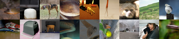
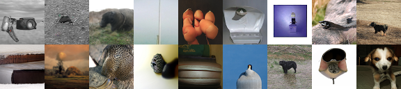
Figure 5: More unconditional samples from MD4 trained on ImageNet 64x64.

In all experiments, the model is trained with a continuous-time loss while samples are drawn from the discrete-time reverse model of 1000 timesteps unless otherwise noted. We used an exponential moving average factor 0.9999 for all evaluation including sample generation.

H.1 text8

We followed the standard dataset split as in Austin et al. [14], Lou et al. [32] and trained our models on text chunks of length 256 for 1 million steps with batch size 512. All models in the table used a standard 12-layer transformer architecture unless otherwise noted. Our transformer has also the same number of heads (12) and hidden dimension (784) as in Austin et al. [14], Lou et al. [32].

We used the continuous-time ELBO and drew one sample of $t$ for each data to estimate the integral. To reduce the variance of training, we used the same antithetic sampling trick described in Kingma et al. [33] for continuous diffusion models. We used the linear masking schedule $\alpha_{t}=1-t$ and added a small shift $\epsilon=10^{-4}$ when $t$ is close to $0$ and $1$ to ensure numerical stability. The shifted schedule is $\alpha_{t}=(1-2\epsilon)(1-t)+\epsilon$. The shift leads to a support mismatch between $q(x_{1}|x_{0})$ and the prior $p(x_{1})$, leading to an undefined KL divergence term. We explain in appendix E how to modify the prior distribution to allow small uniform probabilities in non-mask states to mitigate this problem. The shift leads to a non-zero reconstruction term and KL divergence term for the prior distribution but both are of negligible scale so we can safely ignore them when reporting the ELBO.

We used a cosine learning rate schedule with a linear warm up of 2000 steps. We applied channel-wise dropout of rate $0.05$ and used AdamW optimizer with learning rate 0.0003 and a weight decay factor of 0.03. Our model is trained on 16 TPU-v5 lite for less than a day.

H.2 OpenWebText

Additional unconditional generation from our MD4 Medium model is shown in Appendix I.

We kept 2% of the original training set for validation. Our small and medium transformer model have the same number of layers, heads, and hidden dimensions as in Lou et al. [32] and our tokenizer was also kept the same with a vocabulary size of around 50K. The training objective, masking schedule and other architectural choices were kept the same with the text8 experiment. We kept the training hyperparameters the same as text8 experiment except that we reduced the dropout rate to 0.02.

H.3 Images

Additional unconditional generation from our MD4 model is presented in Figure 5.

We used the same linear masking schedule as in previous experiments in all reported results. We have observed that the cosine schedule leads to better sample quality so we used it instead for visualizing samples from the model.

We used the same U-Net plus self-attention architectures from the continuous diffusion model described in Kingma et al. [33] for CIFAR-10, except that we did not use Fourier feature inputs and added an additional input embedding layer with embedding size the same as the hidden dimension of the model. For ImageNet $64\times 64$, we reduced the number of residual blocks from 64 to 48 and add 12 additional diffusion transformer [64] blocks with 768 hidden dimension and 12 heads in the middle.

We used AdamW optimizer with learning rate 0.0002 and weight decay factor 0.01 for both datasets. The learning rate follows a cosine annealing after 100 warm up steps. The batch size is 128 for CIFAR-10 and 512 for ImageNet 64$\times$64. Our CIFAR-10 model is trained on 16 TPU-v5 lite for 24 hours. Our ImageNet-$64\times 64$ model is trained on 256 TPU-v4 for 2 days.

Appendix I Additional unconditional generation from MD4-M

I.1 MD4-M sample 1: 1024 tokens

like, I don’t have to be alive? Sometimes there are things that are too real
and you’re really supposed to experience them. So that’s a good feeling.
That is the scary thing. Not actually, being able to experience things, being
able to do these things, when you’re doing them, which, for most people
having to wake in a dream is something that seems the most significant, and then
you think about it the next day. It’s like the hope of the future,
and you wake up right now thinking about it. What happens is,, then you
have to stop and think about it and then all of a sudden, somebody always
says, "You’re dreaming."

And sometimes I wonder if this is a good time to teach your gut instincts to
your actors when you’re doing a show like this. Because even on this particular
show, it feels like everyone’s been through this all the time before, if even
a few years ago. I mean, if you’re doing a show together, at least not on
continuous development, you you’re a vet. I mean, you should really be along.
If you’re not sure, well --

VS: I’m working on that one.

Did any of you guys feel that an instinct could work? I thought, "Well, because
you didn’t do ’Deadwood’ you should stop doing this." But when I read the story
for the first time, I thought, "I think this is going to work." What I can’t
picture is a way to hold this apart.

VS: That’s me. It’s what we have to do. So do we. When we wrote the first episode,
we wrote a script that we felt like me and myself would want to see. I knew that I
wanted to be able to be in something -- and I wanted to be able to take refuge in
something that was real, that you could see and just really step out of yourself.
And then I saw it. Then, you get rehearsing it and doing it. And then I actually
started shooting. I think I knew I didn’t think it was going to be good. But,
I know it was good. And now people are talked about because it’s not good enough.

Growing up, you say that you just completely hated the show, "Lost." Isn’t that
what you wish for at the end of the day?

VS: I don’t like the concept.

And so there’s a lot that you don’t know about that, so I think for me to have had
these ideas, if you didn’t understand even that it was coming out of this world
that doesn’t exist, we might never get together.

It’s so weird. This happened to happen at the same time?

VS: Yes. It happened to happen at basically the same time.

Nobody’s even had a show or had a movie/come out of the movie, but ...

VS: If I’m going to pretend I’m definitely not you and have to live through that
stuff, I don’t think I’m going to swallow that. I didn’t expect it to do quite
that long.

There are always things now that happen with ’Deadwood’ where you don’t know where
it’s going to end up next time, but I think there are occasions now where we have
to keep the fight, even if ’Lost’ was pretty consistent in the mindset and the form.

VS: I’m glad that we did fight the odds, because we should have understood that
there was a direct link. But there was almost a sense of not that we had showed up
on the same day, we know we work in the same pieces, but a lot of stuff we don’t
know about. Some of it, we need to deal with. We also just have to accept the
language, and there are a lot of things where we take from them and we do this
what they did  because we want to

I.2 MD4-M sample 2: 1024 tokens

the groups let recreational vehicles use the three roads that will stay open in
the meantime of fighting off the permit. "The purpose of the permit is to make
sure that we work with  the NPS and made roadways and rest areas. We’re not just
scaring guys kind of messing around." Community plans to build an urban bike
facility marched forward at the ongoing staff meeting of the King County
Commission.

Trail will be finished just south of the Greenview 5.

Instead of continuing with a pedestrian and bike trail to the MBTA’s campus, these
two trails could bridle the areas from Market to 14 and carry communities closer.

"This project will provide a car-free path to King County," said Andrew Weed. It’s
been put the brakes on in the past several months, but there are those residents
still skeptical.

"I’ve addressed some of the community concerns that’ve been raised. They’ve
expressed some of their concerns. I dont think it’s terribly reasonable from a
transportation standpoint."

The trail had been set up to meet on for more than a year when the council
approved funding for a different proposal.

Mayor Muriel Bowser said after meetings with Commissioner Bushell on Thursday that
the new plan will be on board in December.

"Theres enough of a finish for this project to roll out on time, and were going
to get it done," Bowser said.

For the public, the campaign appears over.

There was one meeting that I feel like I lost at last night’s meeting," said
Shelley Potts, a local resident.

Local resident Joel Grimy, who lives on Uman Road, met residents there as well.

And in other groups that rode through Mayor assistant Stacey Land and even her son
held fliers saying to look for light sign, and also met with Bowsers son, Deion
Bowser, about a future plan to also have a dog park on the transit corridor.

Advocates at Brickleys event, many one waited at least 11 minutes in during the
start of the public meeting, said they expect at least another month from the
Board of Commissioners, even after a public hearing on Nov. 13.

"We’ve been trying to be a talkative board where we are meeting in advance, being
respectful of folks," Bowser said.

He considered that the proposal for the section of trail between the Greenview 5
and 3 has to move on a schedule. We have other historic preservation projects
that would take over that.

But Chad Routledge, a local advocate of the project, spoke out against the mayors
plan.

The mayor has sent a new meeting to the public using the same route that resulted
from the loud criticism and onslaught of complaints from the community committee
back during the public hearing, Routledge said.

The BDC doesnt have a particular plan-turns around for the end of the planned
path, and says nothing practical can happen right now. But, she said the agency
still "looking to make investments in facilities along the route."

And still there is another part of the trail that might be just as much a wish for
the dogs, as cars: the district wants to go west foot a couple blocks south, to
make the trail safer for dogs.

I feel that the accessibility of the trail is pretty important. I think the
education of the trail, and the uses along different routes are very important
pieces of a balanced outcome, said Bushell.

Trams coming off Route 1

References

- Sohl-Dickstein et al. [2015] Jascha Sohl-Dickstein, Eric Weiss, Niru Maheswaranathan, and Surya Ganguli. Deep unsupervised learning using nonequilibrium thermodynamics. In International Conference on Machine Learning, 2015.
- Ho et al. [2020] Jonathan Ho, Ajay Jain, and Pieter Abbeel. Denoising diffusion probabilistic models. In Advances in Neural Information Processing Systems, 2020.
- Song et al. [2020] Yang Song, Jascha Sohl-Dickstein, Diederik P Kingma, Abhishek Kumar, Stefano Ermon, and Ben Poole. Score-based generative modeling through stochastic differential equations. In International Conference on Learning Representations, 2020.
- Rombach et al. [2022] Robin Rombach, Andreas Blattmann, Dominik Lorenz, Patrick Esser, and Björn Ommer. High-resolution image synthesis with latent diffusion models. In Proceedings of the IEEE/CVF Conference on Computer Vision and Pattern Recognition, pages 10684–10695, 2022.
- Ramesh et al. [2022] Aditya Ramesh, Prafulla Dhariwal, Alex Nichol, Casey Chu, and Mark Chen. Hierarchical text-conditional image generation with clip latents. arXiv preprint arXiv:2204.06125, 1(2):3, 2022.
- Saharia et al. [2022] Chitwan Saharia, William Chan, Saurabh Saxena, Lala Li, Jay Whang, Emily L Denton, Kamyar Ghasemipour, Raphael Gontijo Lopes, Burcu Karagol Ayan, Tim Salimans, et al. Photorealistic text-to-image diffusion models with deep language understanding. In Advances in Neural Information Processing Systems, 2022.
- Chen et al. [2021] Nanxin Chen, Yu Zhang, Heiga Zen, Ron J Weiss, Mohammad Norouzi, and William Chan. Wavegrad: Estimating gradients for waveform generation. In International Conference on Learning Representations, 2021.
- Kong et al. [2021] Zhifeng Kong, Wei Ping, Jiaji Huang, Kexin Zhao, and Bryan Catanzaro. Diffwave: A versatile diffusion model for audio synthesis. In International Conference on Learning Representations, 2021.
- Ho et al. [2022] Jonathan Ho, Tim Salimans, Alexey Gritsenko, William Chan, Mohammad Norouzi, and David J Fleet. Video diffusion models. In Advances in Neural Information Processing Systems, 2022.
- Villegas et al. [2023] Ruben Villegas, Mohammad Babaeizadeh, Pieter-Jan Kindermans, Hernan Moraldo, Han Zhang, Mohammad Taghi Saffar, Santiago Castro, Julius Kunze, and Dumitru Erhan. Phenaki: Variable length video generation from open domain textual descriptions. In International Conference on Learning Representations, 2023.
- Bar-Tal et al. [2024] Omer Bar-Tal, Hila Chefer, Omer Tov, Charles Herrmann, Roni Paiss, Shiran Zada, Ariel Ephrat, Junhwa Hur, Yuanzhen Li, Tomer Michaeli, et al. Lumiere: A space-time diffusion model for video generation. arXiv preprint arXiv:2401.12945, 2024.
- OpenAI [2024] OpenAI. Sora. https://openai.com/index/sora/, 2024.
- Bao et al. [2024] Fan Bao, Chendong Xiang, Gang Yue, Guande He, Hongzhou Zhu, Kaiwen Zheng, Min Zhao, Shilong Liu, Yaole Wang, and Jun Zhu. Vidu: a highly consistent, dynamic and skilled text-to-video generator with diffusion models. arXiv preprint arXiv:2405.04233, 2024.
- Austin et al. [2021] Jacob Austin, Daniel D Johnson, Jonathan Ho, Daniel Tarlow, and Rianne Van Den Berg. Structured denoising diffusion models in discrete state-spaces. In Advances in Neural Information Processing Systems, 2021.
- Hoogeboom et al. [2021a] Emiel Hoogeboom, Didrik Nielsen, Priyank Jaini, Patrick Forré, and Max Welling. Argmax flows and multinomial diffusion: Learning categorical distributions. In Advances in Neural Information Processing Systems, 2021a.
- Vignac et al. [2023] Clément Vignac, Igor Krawczuk, Antoine Siraudin, Bohan Wang, Volkan Cevher, and Pascal Frossard. DiGress: Discrete denoising diffusion for graph generation. In International Conference on Learning Representations, 2023.
- Yang et al. [2023] Dongchao Yang, Jianwei Yu, Helin Wang, Wen Wang, Chao Weng, Yuexian Zou, and Dong Yu. Diffsound: Discrete diffusion model for text-to-sound generation. IEEE/ACM Transactions on Audio, Speech, and Language Processing, 2023.
- Gruver et al. [2023] Nate Gruver, Samuel Stanton, Nathan Frey, Tim GJ Rudner, Isidro Hotzel, Julien Lafrance-Vanasse, Arvind Rajpal, Kyunghyun Cho, and Andrew G Wilson. Protein design with guided discrete diffusion. In Advances in Neural Information Processing Systems, 2023.
- Dieleman et al. [2022] Sander Dieleman, Laurent Sartran, Arman Roshannai, Nikolay Savinov, Yaroslav Ganin, Pierre H Richemond, Arnaud Doucet, Robin Strudel, Chris Dyer, Conor Durkan, et al. Continuous diffusion for categorical data. arXiv preprint arXiv:2211.15089, 2022.
- Chen et al. [2022] Ting Chen, Ruixiang ZHANG, and Geoffrey Hinton. Analog bits: Generating discrete data using diffusion models with self-conditioning. In International Conference on Learning Representations, 2022.
- Li et al. [2022] Xiang Li, John Thickstun, Ishaan Gulrajani, Percy S Liang, and Tatsunori B Hashimoto. Diffusion-LM improves controllable text generation. In Advances in Neural Information Processing Systems, 2022.
- Gulrajani and Hashimoto [2023] Ishaan Gulrajani and Tatsunori B Hashimoto. Likelihood-based diffusion language models. In Advances in Neural Information Processing Systems, 2023.
- Lovelace et al. [2024] Justin Lovelace, Varsha Kishore, Chao Wan, Eliot Shekhtman, and Kilian Q Weinberger. Latent diffusion for language generation. In Advances in Neural Information Processing Systems, 2024.
- Richemond et al. [2022] Pierre H Richemond, Sander Dieleman, and Arnaud Doucet. Categorical SDEs with simplex diffusion. arXiv preprint arXiv:2210.14784, 2022.
- Avdeyev et al. [2023] Pavel Avdeyev, Chenlai Shi, Yuhao Tan, Kseniia Dudnyk, and Jian Zhou. Dirichlet diffusion score model for biological sequence generation. In International Conference on Machine Learning, 2023.
- Graves et al. [2023] Alex Graves, Rupesh Kumar Srivastava, Timothy Atkinson, and Faustino Gomez. Bayesian flow networks. arXiv preprint arXiv:2308.07037, 2023.
- Xue et al. [2024] Kaiwen Xue, Yuhao Zhou, Shen Nie, Xu Min, Xiaolu Zhang, Jun Zhou, and Chongxuan Li. Unifying Bayesian flow networks and diffusion models through stochastic differential equations. arXiv preprint arXiv:2404.15766, 2024.
- Liu et al. [2024] Guan-Horng Liu, Tianrong Chen, Evangelos Theodorou, and Molei Tao. Mirror diffusion models for constrained and watermarked generation. In Advances in Neural Information Processing Systems, 2024.
- Campbell et al. [2022] Andrew Campbell, Joe Benton, Valentin De Bortoli, Thomas Rainforth, George Deligiannidis, and Arnaud Doucet. A continuous time framework for discrete denoising models. In Advances in Neural Information Processing Systems, 2022.
- Chang et al. [2022] Huiwen Chang, Han Zhang, Lu Jiang, Ce Liu, and William T Freeman. Maskgit: Masked generative image transformer. In Proceedings of the IEEE/CVF Conference on Computer Vision and Pattern Recognition, 2022.
- Zheng et al. [2023] Lin Zheng, Jianbo Yuan, Lei Yu, and Lingpeng Kong. A reparameterized discrete diffusion model for text generation. arXiv preprint arXiv:2302.05737, 2023.
- Lou et al. [2024] Aaron Lou, Chenlin Meng, and Stefano Ermon. Discrete diffusion language modeling by estimating the ratios of the data distribution. In International Conference on Machine Learning, 2024.
- Kingma et al. [2021] Diederik Kingma, Tim Salimans, Ben Poole, and Jonathan Ho. Variational diffusion models. In Advances in Neural Information Processing Systems, 2021.
- Karras et al. [2022] Tero Karras, Miika Aittala, Timo Aila, and Samuli Laine. Elucidating the design space of diffusion-based generative models. In Advances in Neural Information Processing Systems, 2022.
- Benton et al. [2024] Joe Benton, Yuyang Shi, Valentin De Bortoli, George Deligiannidis, and Arnaud Doucet. From denoising diffusions to denoising Markov models. Journal of the Royal Statistical Society Series B: Statistical Methodology, 86(2):286–301, 2024.
- Zhao et al. [2024] Lingxiao Zhao, Xueying Ding, Lijun Yu, and Leman Akoglu. Improving and unifying discrete and continuous-time discrete denoising diffusion. arXiv preprint arXiv:2402.03701, 2024.
- Campbell et al. [2024] Andrew Campbell, Jason Yim, Regina Barzilay, Tom Rainforth, and Tommi Jaakkola. Generative flows on discrete state-spaces: Enabling multimodal flows with applications to protein co-design. In International Conference on Machine Learning, 2024.
- Shi et al. [2022] Jiaxin Shi, Yuhao Zhou, Jessica Hwang, Michalis Titsias, and Lester Mackey. Gradient estimation with discrete Stein operators. In Advances in Neural Information Processing Systems, 2022.
- Salimans and Knowles [2014] Tim Salimans and David A Knowles. On using control variates with stochastic approximation for variational bayes and its connection to stochastic linear regression. arXiv preprint arXiv:1401.1022, 2014.
- Kool et al. [2019] W. Kool, H. V. Hoof, and M. Welling. Buy 4 REINFORCE samples, get a baseline for free! In DeepRLStructPred@ICLR, 2019.
- [41] Matt Mahoney. Text8. https://mattmahoney.net/dc/textdata.html. Accessed: 2024-05-14.
- Gokaslan and Cohen [2019] Aaron Gokaslan and Vanya Cohen. Openwebtext corpus. http://Skylion007.github.io/OpenWebTextCorpus, 2019.
- Radford et al. [2019] Alec Radford, Jeffrey Wu, Rewon Child, David Luan, Dario Amodei, and Ilya Sutskever. Language models are unsupervised multitask learners. OpenAI blog, 1(8):9, 2019.
- Paperno et al. [2016] Denis Paperno, Germán Kruszewski, Angeliki Lazaridou, Ngoc-Quan Pham, Raffaella Bernardi, Sandro Pezzelle, Marco Baroni, Gemma Boleda, and Raquel Fernández. The lambada dataset: Word prediction requiring a broad discourse context. In Proceedings of the 54th Annual Meeting of the Association for Computational Linguistics (Volume 1: Long Papers), pages 1525–1534, 2016.
- Marcus et al. [1993] Mitch Marcus, Beatrice Santorini, and Mary Ann Marcinkiewicz. Building a large annotated corpus of english: The penn treebank. Computational Linguistics, 19(2):313–330, 1993.
- Merity et al. [2016] Stephen Merity, Caiming Xiong, James Bradbury, and Richard Socher. Pointer sentinel mixture models. In International Conference on Learning Representations, 2016.
- Chelba et al. [2014] Ciprian Chelba, Tomas Mikolov, Mike Schuster, Qi Ge, Thorsten Brants, Phillipp Koehn, and Tony Robinson. One billion word benchmark for measuring progress in statistical language modeling. In Interspeech, 2014.
- Hoogeboom et al. [2021b] Emiel Hoogeboom, Alexey A Gritsenko, Jasmijn Bastings, Ben Poole, Rianne van den Berg, and Tim Salimans. Autoregressive diffusion models. In International Conference on Learning Representations, 2021b.
- Shih et al. [2022] Andy Shih, Dorsa Sadigh, and Stefano Ermon. Training and inference on any-order autoregressive models the right way. In Advances in Neural Information Processing Systems, 2022.
- Ziegler and Rush [2019] Zachary Ziegler and Alexander Rush. Latent normalizing flows for discrete sequences. In International Conference on Machine Learning, 2019.
- Tran et al. [2019] Dustin Tran, Keyon Vafa, Kumar Agrawal, Laurent Dinh, and Ben Poole. Discrete flows: Invertible generative models of discrete data. In Advances in Neural Information Processing Systems, 2019.
- Van Den Oord et al. [2016] Aäron Van Den Oord, Nal Kalchbrenner, and Koray Kavukcuoglu. Pixel recurrent neural networks. In International Conference on Machine Learning, 2016.
- Van den Oord et al. [2016] Aaron Van den Oord, Nal Kalchbrenner, Lasse Espeholt, Oriol Vinyals, and Alex Graves. Conditional image generation with pixelcnn decoders. In Advances in Neural Information Processing systems, 2016.
- Salimans et al. [2016] Tim Salimans, Andrej Karpathy, Xi Chen, and Diederik P Kingma. Pixelcnn++: Improving the pixelcnn with discretized logistic mixture likelihood and other modifications. In International Conference on Learning Representations, 2016.
- Chen et al. [2018] Xi Chen, Nikhil Mishra, Mostafa Rohaninejad, and Pieter Abbeel. Pixelsnail: An improved autoregressive generative model. In International Conference on Machine Learning, 2018.
- Parmar et al. [2018] Niki Parmar, Ashish Vaswani, Jakob Uszkoreit, Lukasz Kaiser, Noam Shazeer, Alexander Ku, and Dustin Tran. Image transformer. In International Conference on Machine Learning, 2018.
- Child et al. [2019] Rewon Child, Scott Gray, Alec Radford, and Ilya Sutskever. Generating long sequences with sparse transformers. arXiv preprint arXiv:1904.10509, 2019.
- Roy et al. [2021] Aurko Roy, Mohammad Saffar, Ashish Vaswani, and David Grangier. Efficient content-based sparse attention with routing transformers. Transactions of the Association for Computational Linguistics, 9:53–68, 2021.
- Savinov et al. [2022] Nikolay Savinov, Junyoung Chung, Mikolaj Binkowski, Erich Elsen, and Aaron van den Oord. Step-unrolled denoising autoencoders for text generation. In International Conference on Learning Representations, 2022.
- Han et al. [2024] Kehang Han, Kathleen Kenealy, Aditya Barua, Noah Fiedel, and Noah Constant. Transfer learning for text diffusion models. arXiv preprint arXiv:2401.17181, 2024.
- Bengio et al. [2015] Samy Bengio, Oriol Vinyals, Navdeep Jaitly, and Noam Shazeer. Scheduled sampling for sequence prediction with recurrent neural networks. In Advances in Neural Information Processing Systems, 2015.
- Glynn [1990] Peter W. Glynn. Likelihood ratio gradient estimation for stochastic systems. Communications of the ACM, 33(10):75–84, 1990.
- Williams [1992] Ronald J Williams. Simple statistical gradient-following algorithms for connectionist reinforcement learning. Machine Learning, 8(3-4):229–256, 1992.
- Peebles and Xie [2023] William Peebles and Saining Xie. Scalable diffusion models with transformers. In Proceedings of the IEEE/CVF International Conference on Computer Vision, pages 4195–4205, 2023.