Shield Synthesis for LTL Modulo Theories

Abstract

In recent years, Machine Learning (ML) models have achieved remarkable success in various domains. However, these models also tend to demonstrate unsafe behaviors, precluding their deployment in safety-critical systems. To cope with this issue, ample research focuses on developing methods that guarantee the safe behaviour of a given ML model. A prominent example is shielding which incorporates an external component (a “shield”) that blocks unwanted behavior. Despite significant progress, shielding suffers from a main setback: it is currently geared towards properties encoded solely in propositional logics (e.g., LTL) and is unsuitable for richer logics. This, in turn, limits the widespread applicability of shielding in many real-world systems. In this work, we address this gap, and extend shielding to LTL modulo theories, by building upon recent advances in reactive synthesis modulo theories. This allowed us to develop a novel approach for generating shields conforming to complex safety specifications in these more expressive, logics. We evaluated our shields and demonstrate their ability to handle rich data with temporal dynamics. To the best of our knowledge, this is the first approach for synthesizing shields for such expressivity.

1 Introduction

Recently, DNN-based agents trained using Deep Reinforcement Learning (DRL) have been shown to successfully control reactive systems of high complexity (e.g., (?)) , such as robotic platforms. However, despite their success, DRL controllers still suffer from various safety issues; e.g., small perturbations to their inputs, resulting either from noise or from a malicious adversary, can cause even state-of-the-art agents to react unexpectedly (e.g., (?)) . This issue raises severe concerns regarding the deployment of DRL-based agents in safety-critical reactive systems.

In order to cope with these DNN reliability concerns, the formal methods community has recently put forth various tools and techniques that rigorously ensure the safe behaviour of DNNs (e.g., (?)) , and specifically, of DRL-controlled reactive systems (e.g., (?)) . One of the main approaches that is gaining popularity, is shielding (?; ?), i.e., the incorporation of an external component (a “shield”) that forces an agent to behave safely according to a given specification. This specification $\varphi$ is usually expressed as a propositional formula, in which the atomic propositions represent the inputs ($I$) and outputs ($O$) of the system, controlled by the DNN in question. Once $\varphi$ is available, shielding seeks to guarantee that all behaviors of the given system $D$ satisfy $\varphi$ through the means of a shield $S$: whenever the system encounters an input $I$ that triggers an erroneous output (i.e., $O:D(I)$ for which $\varphi(I,O)$ does not hold), $S$ corrects $O$ and replaces it with another action $O^{\prime}$, to ensure that $\varphi$(I, O’) does hold. Thus, the combined system $D\cdot S$ never violates $\varphi$. Shields are appealing for multiple reasons: they do not require “white box” access to $D$, a single shield $S$ can be used for multiple variants of $D$, it is usually computationally cheaper than static methods like DNN verification etc. Moreover, shields are intuitive for practitioners, since they are synthesized based on the required $\varphi$. However, despite significant progress, modern shielding methods still suffer from a main setback: they are only applicable to specifications in which the inputs/outputs are over Boolean atomic propositions. This allows users to encode only discrete specifications, typically in Linear Temporal Logic (LTL). Thus, as most real-world systems rely on rich data specifications, this precludes the use of shielding in various such domains, such as continuous input spaces.

In this work, we address this gap and present a novel approach for shield synthesis that makes use of LTL modulo theories ($\textup{LTL}_{\mathcal{T}}$), where Boolean propositions are extended to literals from a (multi-sorted) first-order theory $\mathcal{T}$. Concretely, we leverage Boolean abstraction methods (?), which transform $\textup{LTL}_{\mathcal{T}}$ specifications into equi-realizable pure (Boolean) LTL specifications. We combine Boolean abstraction with reactive $\textup{LTL}_{\mathcal{T}}$ synthesis (?), extending the common LTL shielding theory into a $\textup{LTL}_{\mathcal{T}}$ shielding theory. Using $\textup{LTL}_{\mathcal{T}}$ shielding, we are able to construct shields for more expressive specifications. This, in turn, allows us to override unwanted actions in a (possibly infinite) domain of $\mathcal{T}$, and guarantee the safety of DNN-controlled systems in such complex scenarios. In summary, our contributions are: (1) developing two methods for shield synthesis over $\textup{LTL}_{\mathcal{T}}$ and presenting their proof of correctness; (2) an analysis of the impact of the Boolean abstractions in the precision of shields; (3) a formalization of how to construct optimal shields using objective functions; and (4) an empirical evaluation that shows the applicability of our techniques.

2 Preliminaries

LTL and $\textup{LTL}_{\mathcal{T}}$.

We start from LTL (?; ?), which has the following syntax:

$$\varphi::=\top\hskip 1.99997pt\big{|}\hskip 1.99997pta\hskip 1.99997pt\big{|}\hskip 1.99997pt\varphi\lor\varphi\hskip 1.99997pt\big{|}\hskip 1.99997pt\neg\varphi\hskip 1.99997pt\big{|}\hskip 1.99997pt\LTLcircle\varphi\hskip 1.99997pt\big{|}\hskip 1.99997pt\varphi\mathbin{\mathcal{U}}\varphi,$$

where $a\in\mathsf{AP}$ is an atomic proposition, $\{\land,\neg\}$ are the common Boolean operators of conjunction and negation, respectively, and $\{\LTLcircle,\mathbin{\mathcal{U}}\}$ are the next and until temporal operators, respectively. Additional temporal operators include $\mathcal{R}$ (release), (finally), and (always), which can be derived from the syntax above. Given a set of atomic propositions $\overline{a}$ we use $\textit{val}(\overline{a})$ for a set of possible valuations of variables in $\overline{a}$ (i.e. $\textit{val}(\overline{a})=2^{\overline{a}}$), and we use $v_{\overline{a}}$ to range over $\textit{val}(\overline{a})$. We use $\Sigma=\textit{val}(\mathsf{AP})$. The semantics of LTL formulas associates traces $\sigma\in\Sigma^{\omega}$ with LTL fomulas (where $\sigma\models\top$ always holds, and $\mathrel{\vee}$ and $\neg$ are standard):

$$\begin{array}[]{l@{\hspace{0.3em}}c@{\hspace{0.3em}}l}\sigma\models a\hfil\hskip 3.00003pt&\text{iff }\hfil\hskip 3.00003pt&a\in\sigma(0)\\ \sigma\models\LTLcircle\varphi\hfil\hskip 3.00003pt&\text{iff }\hfil\hskip 3.00003pt&\sigma^{1}\models\varphi\\ \sigma\models\varphi_{1}\mathbin{\mathcal{U}}\varphi_{2}\hfil\hskip 3.00003pt&\text{iff }\hfil\hskip 3.00003pt&\text{for some }i\geq 0\;\;\sigma^{i}\models\varphi_{2},\text{ and }\\ \hfil\hskip 3.00003pt&\hfil\hskip 3.00003pt&\;\;\;\;\;\text{for all }\text{for all }0\leq j<i,\sigma^{j}\models\varphi_{1}\\ \end{array}$$

A safety formula $\varphi$ is such that for every failing trace $\sigma\not\models\varphi$ there is a finite prefix $u$ of $\sigma$, such that all $\sigma^{\prime}$ extending $u$ also falsify $\varphi$ (i.e. $\sigma^{\prime}\not\models\varphi$).

The syntax of LTL modulo theory ($\textup{LTL}_{\mathcal{T}}$) replaces atoms $a$ by literals $l$ from some theory $\mathcal{T}$. Even though we use multi-sorted theories, for clarity of explanation we assume that $\mathcal{T}$ has only one sort and use $\mathbb{D}$ for the domain, the set that populates the sort of its variables. For example, the domain of linear integer arithmetic $\mathcal{T}_{\mathbb{Z}}$ is $\mathbb{Z}$ and we denote this by $\mathbb{D}(\mathcal{T}_{\mathbb{Z}})=\mathbb{Z}$. Given an $\textup{LTL}_{\mathcal{T}}$ formula $\varphi(\overline{z})$ with variables $\overline{z}$ the semantics of $\textup{LTL}_{\mathcal{T}}$ now associate traces $\sigma$ (where each letter is a valuation of $\overline{z}$, i.e., a mapping from $\overline{z}$ into $\mathbb{D}$) with $\textup{LTL}_{\mathcal{T}}$ formulae. The semantics of the Boolean and temporal operators are as in LTL, and for literals:

$$\begin{array}[]{l@{\hspace{0.3em}}c@{\hspace{0.3em}}l@{\hspace{0em}}}\sigma\models l\hfil\hskip 3.00003pt&\text{iff }\hfil\hskip 3.00003pt&\text{the valuation $\sigma(0)$ of $\overline{z}$ makes $l$ true according to $\mathcal{T}$}\\ \end{array}$$

The Synthesis Problem.

Reactive LTL synthesis (?; ?) is the task of producing a system that satisfies a given LTL specification $\varphi$, where atomic propositions in $\varphi$ are split into variables controlled by the environment (“input variables”) and by the system (“output variables”), denoted by $\overline{e}$ and $\overline{s}$, respectively. Synthesis corresponds to a game where, in each turn, the environment player produces values for the input propositions, and the system player responds with values of the output propositions. A play is an infinite sequence of turns, i.e., an infinite interaction of the system with the environment. A strategy for the system is a tuple $C_{\mathbb{B}}:\langle Q,q_{0},\delta,o\rangle$ where $Q$ is a finite set of states, $q_{0}\in Q$ is the inital state, $\delta:Q\times\textit{val}(\overline{e})\mathrel{\rightarrow}Q$ is the transition function and $o:Q\times\textit{val}(\overline{e})\mathrel{\rightarrow}\textit{val}(\overline{s})$ is the output function. $C_{\mathbb{B}}$ is said to be winning for the system if all the possible plays played according to the strategy satisfy the LTL formula $\varphi_{\mathbb{B}}$. In this paper we use “strategy” and “controller” interchangeably.

We also introduce the notion of winning region (WR), which encompasses all possible winning moves for the system in safety formulae. A winning region $\textit{WR}:\langle Q,I,T\rangle$ is a tuple where $Q$ is a finite set of states, $I\subseteq Q$ is a set of initial states and $T:Q\times\textit{val}(\overline{e})\mathrel{\rightarrow}{}2^{(Q\times\textit{val}(\overline{s}))}$ is the transition relation, which provides for a given state $q$ and input $v_{\overline{e}}$, all the possible pairs of legal successor and output $(q^{\prime},v_{\overline{s}})$. For a safety specification, every winning strategy is “included” into the WR (i.e., there is an embedding map). LTL realizability is the decision problem of whether there is a winning strategy for the system (i.e., check whether $\text{WR}\neq\emptyset$), while LTL synthesis is the computational problem of producing one.

However, in $\textup{LTL}_{\mathcal{T}}$ synthesis (?; ?), the specification is expressed in a richer logic where propositions are replaced by literals from some $\mathcal{T}$. In $\textup{LTL}_{\mathcal{T}}$ the (first order) variables in specification $\varphi_{\mathcal{T}}$ are still split into those controlled by the environment ($\overline{x}$), and those controlled by the system ($\overline{y}$), where $\overline{x}\cap\overline{y}=\emptyset$. We use $\varphi_{\mathcal{T}}(\overline{x},\overline{y})$ to empasize that $\overline{x}\cup\overline{y}$ are all the variables occurring in $\varphi_{\mathcal{T}}$. The alphabet is now $\Sigma_{\mathcal{T}}=\textit{val}(\overline{x}\cup\overline{y})$ (note that now valuations map a variable $x$ to $\mathbb{D}(\mathcal{T})$). We denote by $t[\overline{x}\leftarrow v_{\overline{x}}]$, the substitution in $t$ of variables $\overline{x}$ by values $v_{\overline{x}}$ (similarly for $t[\overline{y}\leftarrow v_{\overline{y}}]$), and also $t[\overline{e}\leftarrow v_{\overline{e}}]$ and $t[\overline{s}\leftarrow v_{\overline{s}}]$ for Boolean variables (propositions). A trace $\pi$ is an infinite sequence of valuations in $\mathbb{D}(\mathcal{T})$, which induces an infinite sequence of Boolean values of the literals occurring in $\varphi_{\mathcal{T}}$ and, in turn, an evaluation of $\varphi_{\mathcal{T}}$ using the semantics of the temporal operators. For example, given $\psi=\LTLsquare(y<x)$ the trace $\pi$ $\{(x:2,y:6),(x:15,y:27)\ldots\}$ induces $\{(\textit{false}),(\textit{true})\ldots\}$. We use $\pi_{x}$ to denote the projection of $\pi$ to the values of only $x$ (resp. $\pi_{y}$ for $y$). A strategy or controller for the system in $\mathcal{T}$ is now a tuple $C_{\mathcal{T}}:\langle Q,q_{0},\delta,o\rangle$ where $Q$ and $q_{0}\in Q$ are as before, and $\delta:Q\times\textit{val}(\overline{x})\mathrel{\rightarrow}Q$ and $o:Q\times\textit{val}(\overline{x})\mathrel{\rightarrow}\textit{val}(\overline{y})$.

Boolean Abstraction.

Boolean abstraction (?) transforms an $\textup{LTL}_{\mathcal{T}}$ specification $\varphi_{\mathcal{T}}$ into an LTL specification $\varphi_{\mathbb{B}}$ in the same temporal fragment (e.g., safety to safety) that preserves realizability, i.e., $\varphi_{\mathcal{T}}$ and $\varphi_{\mathbb{B}}$ are equi-realizable. Then, $\varphi_{\mathbb{B}}$ can be fed into an off-the-shelf synthesis engine, which generates a controller or a WR for realizable instances. Boolean abstraction transforms $\varphi_{\mathcal{T}}$, which contains literals $l_{i}$, into $\varphi_{\mathbb{B}}=\varphi_{\mathcal{T}}[l_{i}\leftarrow s_{i}]\wedge\varphi^{\textit{extra}}$, where $\overline{s}=\{s_{i}|\text{for each }l_{i}\}$ is a set of fresh atomic propositions controlled by the system—such that $s_{i}$ replaces $l_{i}$—and where $\varphi^{\textit{extra}}$ is an additional sub-formula that captures the dependencies between the $\overline{s}$ variables. The formula $\varphi^{\textit{extra}}$ also includes additional variables $\overline{e}$ (controlled by the environment) that encode that the environment can leave the system with the power to choose certain valuations of the variables $\overline{s}$.

We often represent a valuation $v_{\overline{s}}$ of the Boolean variables $\overline{s}$ (which map each variable in $\overline{s}$ to true or false) as a choice $c$ (an element of $2^{\overline{s}}$), where $s_{i}\in c$ means that $v_{\overline{s}}(s_{i})=\textit{true}$. The characteristic formula $f_{c}(\overline{x},\overline{y})$ of a choice $c$ is $f_{c}=\bigwedge_{s_{i}\in c}l_{i}\mathrel{\wedge}\bigwedge_{s_{i}\notin c}\neg l_{i}.$ We use $\mathcal{C}$ for the set of choices, i.e., sets of sets of $\overline{s}$. A reaction $r\subset\mathcal{C}$ is a set of choices, which characterizes the possible responses of the system as the result to a move of the environment. The characteristic formula $f_{r}(\overline{x})$ of a reaction $r$ is: $(\bigwedge_{c\in r}\exists\overline{y}.f_{c})\mathrel{\wedge}(\bigwedge_{c\notin r}\forall\overline{y}\neg f_{c})$. We say that $r$ is a valid reaction whenever $\exists\overline{x}.f_{r}(\overline{x})$ is valid. Intuitively, $f_{r}$ states that for some $v_{\overline{x}}$ by the environment, the system can respond with $v_{\overline{y}}$ making the literals in some choice $c\in r$ but cannot respond with $v_{\overline{y}}$ making the literals in choices $c\notin r$. The set VR of valid reactions partitions precisely the moves of the environment in terms of the reaction power left to the system. For each valid reaction $r$ there is a fresh environment variable $e\in\overline{e}$ used in $\varphi^{\textit{extra}}$ to capture the move of the environment that chooses reaction $r$. The formula $f_{r}(\overline{x})[\overline{x}\leftarrow v_{\overline{x}}]$ is true if a given valuation $v_{\overline{x}}$ of $\overline{x}$ is one move of the environment characterized by $r$. The formula $\varphi^{\textit{extra}}$ also constraints the environment such that exactly one of the variables in $\overline{e}$ is true, which forces that the environment chooses precisely one valid reaction $r$ when the variable $e$ that corresponds to $r$ is true.

Example 1 (Running example and abstraction).

Let $\varphi_{\mathcal{T}}=\square(R_{0}\wedge R_{1})$ where:

$$R_{0}:(x<10)\shortrightarrow\LTLcircle(y>9)\hskip 30.00005ptR_{1}:(x\geq 10)\shortrightarrow(y\leq x),$$

where $\overline{x}=\{x\}$ is controlled by the environment and $\overline{y}=\{y\}$ by the system. In integer theory $\mathcal{T}_{\mathbb{Z}}$ this specification is realizable (consider the strategy to always play $y:10$) and the Boolean abstraction first introduces $s_{0}$ to abstract $(x<10)$, $s_{1}$ to abstract $(y>9)$ and $s_{2}$ to abstract $(y\leq x)$. Then $\varphi_{\mathbb{B}}=\varphi^{\prime\prime}\wedge\LTLsquare(\varphi^{\textit{legal}}\mathrel{\rightarrow}\varphi^{\textit{extra}})$ where $\varphi^{\prime\prime}=(s_{0}\shortrightarrow\LTLcircle s_{1})\wedge(\neg s_{0}\shortrightarrow s_{2})$ is a direct abstraction of $\varphi_{\mathcal{T}}$. Finally, $\varphi^{\textit{extra}}$ captures the dependencies between the abstracted variables:

$$\varphi^{\textit{extra}}:\begin{pmatrix}\begin{array}[]{lrcl}\phantom{\wedge}&\big{(}e_{0}&\mathrel{\rightarrow}&\big{(}f_{c_{1}}\vee f_{c_{2}}\big{)}\\[2.70004pt] \wedge&\big{(}e_{0^{+}}&\mathrel{\rightarrow}&\big{(}f_{c_{1}}\vee f_{c_{2}}\vee f_{c_{3}}\big{)}\\[2.70004pt] \wedge&\big{(}\phantom{\neg}e_{1}&\mathrel{\rightarrow}&\big{(}f_{c_{4}}\vee f_{c_{5}}\vee f_{c_{6}}\big{)}\end{array}\end{pmatrix},$$

where $f_{c_{1}}=(s_{0}\wedge s_{1}\wedge\neg s_{2})$, $f_{c_{2}}=(s_{0}\wedge\neg s_{1}\wedge s_{2})$, $f_{c_{3}}=(s_{0}\wedge\neg s_{1}\wedge\neg s_{2})$, $f_{c_{4}}=(\neg s_{0}\wedge s_{1}\wedge s_{2})$, $f_{c_{5}}=(s_{0}\wedge s_{1}\wedge\neg s_{2})$ and $f_{c_{6}}=(\neg s_{0}\wedge\neg s_{1}\wedge s_{2})$ and where $c_{0}=\{s_{0},s_{1},s_{2}\}$, $c_{1}=\{s_{0},s_{1}\}$, $c_{2}=\{s_{0},s_{2}\}$, $c_{3}=\{s_{0}\}$, $c_{4}=\{s_{1},s_{2}\}$, $c_{5}=\{s_{1}\}$, $c_{6}=\{s_{1}\}$ and $c_{7}=\emptyset$. Also, $\overline{e}=\{e_{0},e_{0^{+}},e_{1}\}$ belong to the environment and represent $(x<10)$, $(x<9)$ and $(x\geq 10)$, respectively. $\varphi^{\textit{legal}}:(e_{0}\mathrel{\wedge}\neg e_{1}\mathrel{\wedge}\neg e_{2})\mathrel{\vee}(\neg e_{0}\mathrel{\wedge}e_{1}\mathrel{\wedge}\neg e_{2})\mathrel{\vee}(\neg e_{0}\mathrel{\wedge}\neg e_{1}\mathrel{\wedge}e_{2})$ encodes that $\overline{e}$ characterizes a partition of the (infinite) input valuations of the environment and that only one of the $\overline{e}$ is true in every move; e.g., the valuation $v_{\overline{e}}:\langle e_{0}:\textit{false},e_{0}^{+}:\textit{true},e_{1}:\textit{false}\rangle$ of $\overline{e}$ corresponds to the choice of the environment where only $e_{0}^{+}$ is true (and we use $v_{\overline{e}}:e_{0}^{+}$ for a shorter notation). Sub-formulae such as $(\neg s_{0}\wedge s_{1}\wedge s_{2})$ represent the choices of the system (in this case, $c=\{s_{1},s_{2}\}$), that is, given a decision of the environment (a valuation of $\overline{e}$ that makes exactly one variable $e\in\overline{e}$ true), the system can react with one of the choices $c$ in the disjunction implied by $e$. Note that $f_{c}=\neg(x<2)\wedge(y>1)\wedge(y\leq x)$. Also, note that $c$ can be represented as $v_{\overline{s}}:\langle s_{0}:\textit{false},s_{1}:\textit{true},s_{2}:\textit{true}\rangle$.

3 Shielding with LTL Modulo Theories

In shielding , at every step, the external design $D$ —e.g., a DRL sub-system— produces an output $v_{\overline{s}}$ from a given input $v_{\overline{e}}$ provided by the environment. The pair $(v_{\overline{e}},v_{\overline{s}})$ is passed to the shield $S$ which decides, at every step, whether $v_{\overline{s}}$ proposed by $D$ is safe with respect to some specification $\varphi$. The combined system $D\cdot S$ is guaranteed to satisfy $\varphi$. Using $\textup{LTL}_{\mathcal{T}}$ we can define richer properties than in propositional LTL (which has been previously used in shielding). For instance, consider a classic $D\cdot S$ context in which the $D$ is a robotic navigation platform and $\varphi:\LTLsquare(\texttt{LEFT}\shortrightarrow\LTLcircle\neg\texttt{LEFT})$. Then, if $D$ chooses to turn LEFT after a LEFT action, the shield will consider this second action to be dangerous, and will override it with e.g., RIGHT. If $\textup{LTL}_{\mathcal{T}}$ is used instead of LTL, specifications can be more sophisticated including, for example, numeric data.

Shielding modulo theories is the problem of building a shield $S_{\mathcal{T}}$ from a specification $\varphi_{\mathcal{T}}$ in which at least one of the input variables $\overline{x}$ or one of the output variables $\overline{y}$ are not Boolean.

A shield $S_{\mathcal{T}}$ conforming to $\varphi_{\mathcal{T}}$ will evaluate if a pair $(\overline{x}:v_{\overline{x}},\overline{y}:v_{\overline{y}})$ violates $\varphi_{\mathcal{T}}$ and propose an overriding output $\overline{y}:v_{\overline{y}}^{\prime}$ if so. This way, $D\cdot S_{\mathcal{T}}$ never violates $\varphi_{\mathcal{T}}$. Note that it is possible that $\varphi_{\mathcal{T}}$ is unrealizable, which means that some environment plays will inevitably lead to violations, and hence $S_{\mathcal{T}}$ cannot be constructed, because $\text{WR}=\emptyset$.

Example 2 (Running example as shield).

Recall $\varphi_{\mathcal{T}}$ from Ex. 1. Also, consider $D$ receives an input trace $\pi_{x}=\langle 15,15,7,5,10\rangle$, and produces the output trace $\pi_{y}=\langle 6,5,13,16,11\rangle$. We can see $D$ violates $\varphi_{\mathcal{T}}$ in the fifth step, since $(x<10)$ holds in fourth step (so $v_{y}$ has to be such that $(y:v_{y}>9)$ in the fourth step and $(v_{y}:\leq 10)$ must hold in the fifth step) but $(y:11\leq 10)$ is not true. Instead, a $S_{\mathcal{T}}$ conforming to $\varphi_{\mathcal{T}}$ would notice that $(x:10,y:11)$ violates $\varphi_{\mathcal{T}}$ in this fifth step and would override $v_{y}$ with $v_{y}^{\prime}$ to produce $(y^{\prime}:10)$, which is the only possible valuation of $y^{\prime}$ that does not violate $\varphi_{\mathcal{T}}$. Note that $S_{\mathcal{T}}$ did not intervene in the remaining steps. Thus, $D\cdot S_{\mathcal{T}}$ satisfies $\varphi_{\mathcal{T}}$ in the example.

3.1 $\textup{LTL}_{\mathcal{T}}$ Shield Construction

We propose two different architectures for $S_{\mathcal{T}}$: one following a deterministic strategy and another one that is non-deterministic. Both start from $\varphi_{\mathcal{T}}$ and use Boolean abstraction as the core for the temporal information, but they vary on the way to detect erroneous outputs from $D$ and how to provide corrections.

Shields as Controllers.

The first method leverages $\textup{LTL}_{\mathcal{T}}$ controller synthesis (see Fig. 1(a)) together with a component to detect errors in $D$. The process is as follows, starting from a specification $\varphi_{\mathcal{T}}$:

1. Boolean abstraction (?) transforms $\varphi_{\mathcal{T}}$ into an equi-realizable LTL $\varphi_{\mathbb{B}}$.

2. A Boolean controller $C_{\mathbb{B}}$ is synthesized from $\varphi_{\mathbb{B}}$ (using e.g., (?)). $C_{\mathbb{B}}$ receives Boolean inputs $v_{\overline{e}}$ and provides Boolean outputs $v_{\overline{s}}$.

3. We synthesize a richer controller $C_{\mathcal{T}}$ that receives $v_{\overline{x}}$ and produces outputs $v_{\overline{y}}^{\prime}$ in $\mathbb{D}(\mathcal{T})$. Note the apostrophe in $v_{\overline{y}}^{\prime}$, since $v_{\overline{y}}$ is the output of $D$.

4. $S_{\mathcal{T}}$ receives the output $v_{\overline{y}}$ provided by $D$ and checks if the pair $(v_{\overline{x}},v_{\overline{y}})$ violates $\varphi_{\mathcal{T}}$: if there is a violation, it overrides $v_{\overline{y}}$ with $v_{\overline{y}}^{\prime}$; otherwise, it permits $v_{\overline{y}}$.

We now elaborate on the last steps. To construct $C_{\mathcal{T}}$ from $C_{\mathbb{B}}$ we use (?; ?) , where $C_{\mathcal{T}}$ is composed of three sub-components:

• A partitioner function, which computes Boolean inputs $v_{\overline{e}}$ from the richer inputs $v_{\overline{x}}$ via partitioning, checking whether $f_{r}(v_{\overline{x}})$ is true. Recall that every $v_{\overline{x}}$ is guaranteed to belong to exactly one reaction $r$.

• A Boolean controller $C_{\mathbb{B}}$, which receives $v_{\overline{e}}$ and provides Boolean outputs $v_{\overline{s}}$. Also recall that each Boolean variable in $v_{\overline{s}}$ corresponds exactly to a literal in $\varphi_{\mathcal{T}}$ and that $f_{c}$ is the characteristic formula of $c$.

• A provider, which computes an output $v_{\overline{y}}^{\prime}$ from $f_{c}$ and $r$ such that $v_{\overline{y}}^{\prime}$ is a model of the formula $\exists\overline{y}^{\prime}.\big{(}f_{r}(\overline{x})\mathrel{\rightarrow}f_{c}(\overline{y}^{\prime},\overline{x})\big{)}[\overline{x}\leftarrow v_{\overline{x}}]$.

The composition of the partitioner, $C_{\mathbb{B}}$ and the provider implements $C_{\mathcal{T}}$ (see (?; ?)). For each of these components $g$, let us denote with $g(t_{0})=t_{1}$ the application of $g$ with input $t_{0}$. Then, the following holds:

Lemma 1.

Let $\varphi_{\mathcal{T}}$ be an $\textup{LTL}_{\mathcal{T}}$ specification, $\varphi_{\mathbb{B}}$ its equi-realizable Boolean abstraction and $C_{\mathbb{B}}$ a controller for $\varphi_{\mathbb{B}}$. Let $q$ be a state of $C_{\mathbb{B}}$ after processing inputs $v_{\overline{x}}^{0}\ldots v_{\overline{x}}^{n}$, and let $v_{\overline{x}}$ be the next input from the environment. Let $\textup{{partitioner}}(v_{\overline{x}})=v_{\overline{e}}$ be the partition corresponding to $v_{\overline{x}}$, $o(q,v_{\overline{e}})=v_{\overline{s}}$ be the output of $C_{\mathbb{B}}$ and $c$ be the choice associated to $v_{\overline{s}}$. Then, if $r$ is a valid reaction, the formula $\exists\overline{y}.f_{r}(v_{\overline{x}})\mathrel{\rightarrow}f_{c}(\overline{y},v_{\overline{x}})$ is satisfiable in $\mathcal{T}$, where $c\in r$.

In other words, $C_{\mathcal{T}}$ never has to face with moves from $C_{\mathbb{B}}$ that cannot be mimicked by provider with appropriate values for $v_{\overline{y}}$. Thus, a shield $S_{\mathcal{T}}$ based on $C_{\mathcal{T}}$ (see Fig. 1(a)) first detects whether a valuation pair $(\overline{x}:v_{\overline{x}},\overline{y}:v_{\overline{y}})$ suggested by $D$ violates $\varphi_{\mathcal{T}}$. To do so, at each time-step, $C_{\mathcal{T}}$ obtains $v_{\overline{s}}$ by $C_{\mathbb{B}}$, with associated $c$, and it checks whether $f_{r}(v_{\overline{x}})\mathrel{\rightarrow}f_{c}(v_{\overline{x}},v_{\overline{y}})$ is valid, that is, whether the output proposed is equivalent to the move of $C_{\mathbb{B}}$ (in the sense that every literal $l_{i}$ from $(v_{\overline{x}},v_{\overline{y}})$ has the same valuation $v_{\overline{s}}$ given by $C_{\mathbb{B}}$). If the formula is valid, then $v_{\overline{y}}$ is maintained. Otherwise, the provider is invoked to compute a $v_{\overline{y}}^{\prime}$ that matches the move of $C_{\mathbb{B}}$. In both cases, $S_{\mathcal{T}}$ guarantees that $v_{\overline{s}}$ remains unaltered in $C_{\mathbb{B}}$ and therefore $\varphi_{\mathcal{T}}$ is guaranteed. For instance, in the hypothetical simplistic case where $f_{r}=\textit{true}$, and consider that $C_{\mathbb{B}}$ outputs a $v_{\overline{s}}$ with associated $c$ such that $f_{c}(x,y)=(y>2)\wedge(x<y)$ in $\mathcal{T}_{\mathbb{Z}}$. Then if the input is $x:5$, a candidate output $y:4$ of $D$ would result in $f_{r}(5)\mathrel{\rightarrow}f_{c}(5,4)=(4>2)\wedge(5<4)$, which does not hold. Thus, $y:4$ must be overridden, so $S_{\mathcal{T}}$ will return a model of $\exists y^{\prime}.f_{r}(x)\mathrel{\rightarrow}(y^{\prime}>2)\wedge(x<y^{\prime})[x\leftarrow 5]$. One such possibility is $y^{\prime}:6$.

Lemma 2.

Let $\varphi_{\mathbb{B}}$ be an equi-realizable abstraction of $\varphi_{\mathcal{T}}$, $C_{\mathbb{B}}$ a controller for $\varphi_{\mathbb{B}}$ and $C_{\mathcal{T}}$ a corresponding controller for $\varphi_{\mathcal{T}}$. Also, consider input $v_{\overline{x}}$ and output $v_{\overline{y}}$ by $D$ and $v_{\overline{y}}^{\prime}$ by provider of $C_{\mathcal{T}}$. If both $f_{r}(v_{\overline{x}})\mathrel{\rightarrow}f_{c}(v_{\overline{x}},v_{\overline{y}})$ and $f_{r}(v_{\overline{x}})\mathrel{\rightarrow}f_{c}(v_{\overline{x}},v_{\overline{y}}^{\prime})$ hold, then $v_{\overline{y}}$ and $v_{\overline{y}}^{\prime}$ correspond to the same move of $C_{\mathbb{B}}$.

In other words, if $v_{\overline{y}}$ and $v_{\overline{y}}^{\prime}$ make the same literals true, a shield $S_{\mathcal{T}}$ based on $C_{\mathcal{T}}$ will not override $v_{\overline{y}}$; whereas, otherwise, it will output $v_{\overline{y}}^{\prime}$.

Theorem 1 (Correctness of $D\cdot S_{\mathcal{T}}$ based on $C_{\mathcal{T}}$).

Let $D$ be an external controller and $S_{\mathcal{T}}$ be a shield constructed from a synthetized $C_{\mathcal{T}}$ from a specification $\varphi_{\mathcal{T}}$. Then, $D\cdot S_{\mathcal{T}}$ is also a controller for $\varphi_{\mathcal{T}}$.

In other words, given $\varphi_{\mathcal{T}}$, if $\mathcal{T}$ is decidable in the $\exists^{*}\forall^{*}$-fragment (a condition for the Boolean abstraction (?)), then, leveraging $C_{\mathcal{T}}$, a shield $S_{\mathcal{T}}$ conforming to $\varphi_{\mathcal{T}}$ can be computed for every external $D$ whose input-output domain is $\mathcal{T}$.

More Flexible Shields from Winning Regions.

(a) Using $C_{\mathcal{T}}$ as $S_{\mathcal{T}}$.	(b) Using $W$ as $S_{\mathcal{T}}$.

Figure 1: Architectures for shields modulo theory.

$S_{\mathcal{T}}$ based on $C_{\mathcal{T}}$ are sometimes too intrusive in the sense that they can cause unnecessary corrections, because some $(v_{\overline{x}},v_{\overline{y}})$ may be labelled as a violation when they are not, only because it satisfies a different collection of literals than the ones chosen by the internal controller $C_{\mathbb{B}}$. Given input $v_{\overline{x}}$, the output $v_{\overline{s}}$ provided by $C_{\mathbb{B}}$ and the output $v_{\overline{y}}$ suggest by $D$, $(v_{\overline{x}},v_{\overline{y}})$ is considered to be a dangerous output (i.e., a potential violation of $\varphi_{\mathcal{T}}$) whenever a $f_{r}(v_{\overline{x}})$ holds but the $f_{c}(v_{\overline{x}},v_{\overline{y}})$ of the $c$ associated to $C_{\mathbb{B}}(\textbf{partitioner}(v_{\overline{x}}))=v_{\overline{s}}$ does not hold. Thus, we study now permissive shields $S_{\mathcal{T}}$ with more precise characterizations of unsafe actions.

The winning region (WR) (see Sec. 2) is the most general characterization of the winning states and moves for a safety LTL specification. This second construction can be applied to any subset of WR as long as every state has at least one successor for every input (for example, using the combination of a collection of controllers). The process of computing $S_{\mathcal{T}}$ based on a given winning region $W:\langle Q,I,T\rangle$ is as follows (see Fig. 1(b)), which maintains at each instant a set of current states $Q_{\textit{now}}\subseteq Q$ of $W$, starting from the initial set of states $I$.

1. Compute $\varphi_{\mathbb{B}}$ from $\varphi_{\mathcal{T}}$ using abstraction, as before.

2. We compute the winning region $W$ from $\varphi_{\mathbb{B}}$ (e.g., using (?)).

3. The partitioner computes $v_{\overline{e}}$ from the input values $v_{\overline{x}}$; and, given $v_{\overline{y}}$ provided by $D$, we produce the unique $v_{\overline{s}}$ from $(v_{\overline{x}},v_{\overline{y}})$ or equivalently $c=\{s_{i}|l_{i}(v_{\overline{x}},v_{\overline{y}})\text{ holds}\}$. This is computed by component getchoice in Fig. 1(b).

4. From some of the current states $q\in Q_{\textit{now}}$ maintained, we decide whether $\delta(q,v_{\overline{e}})$ has some successor $(q^{\prime},v_{\overline{s}})$ or not. If it does, output $v_{\overline{y}}$. If it does not, choose a successor output $v_{\overline{s}}^{\prime}$ such that there is $(q^{\prime},v_{\overline{s}}^{\prime})\in\delta(q,v_{\overline{e}})$ for some $q\in Q_{\textit{now}}$, and use a provider to produce an output $v_{\overline{y}}^{\prime}$ (this is implemented by find in Fig. 1(b)). In either case, use appropriate valuation $\overline{v}$ of $\overline{s}$ (i.e., $v_{\overline{s}}$ or $v_{\overline{s}}^{\prime}$) to update $Q_{\textit{now}}$ to $\{q^{\prime}|(q^{\prime},\overline{v})\in\delta(q,v_{\overline{e}})\text{ for some $q\in Q_{\textit{now}}$}\}$.

Note that if the environment generates an input $v_{\overline{x}}$ (with corresponding $v_{\overline{e}}$) and $D$ responds with an output $v_{\overline{y}}$ such that $\textsf{getchoice}(v_{\overline{y}})=v_{\overline{s}}$, if $W$ permits $(v_{\overline{e}},v_{\overline{s}})$ then the suggested $v_{\overline{y}}$ remains. Otherwise, we use a component find which computes an alternative $v_{\overline{s}}^{\prime}$ such that $(v_{\overline{e}},v_{\overline{s}}^{\prime})$ is in $W$ and a proper value $v_{\overline{y}}$ that corresponds to $v_{\overline{s}}$ is output. Also, note that find can always identify a value $v_{\overline{s}}^{\prime}$ from any $q\in Q_{\textit{now}}$ such that there is a successor $(q^{\prime},v_{\overline{s}}^{\prime})\in\delta(q,v_{\overline{e}})$ by the definition of WR. Given two $v_{\overline{s}}$ and $v_{\overline{s}}^{\prime}$ such that $(v_{\overline{e}},v_{\overline{s}})\in W$ and $(v_{\overline{e}},v_{\overline{s}}^{\prime})\in W$, the criteria (e.g., choice-logic (?)) to choose one is not relevant for this paper and we leave it for future work. Finally, given $v_{\overline{x}}$, the $W$ cannot distinguish two values $v_{\overline{y}}$ and $v_{\overline{y}}^{\prime}$ if $\textsf{getchoice}(v_{\overline{x}},v_{\overline{y}})=\textsf{getchoice}(v_{\overline{x}},v_{\overline{y}}^{\prime})$.

Theorem 2 (Correctness of $D\cdot S_{\mathcal{T}}$ based on WR).

Let $\varphi_{\mathcal{T}}$ be a safety specification and $\varphi_{\mathbb{B}}$ obtained from $\varphi_{\mathcal{T}}$ by Boolean abstraction. Let $S_{\mathcal{T}}$ be synthesized using the winning region $W$ of $\varphi_{\mathbb{B}}$. Then, $D\cdot S_{\mathcal{T}}$ satisfies $\varphi_{\mathcal{T}}$, for any external controller $D$.

Thm. 2 holds because the valuations of the literals of any trace $\pi$ of $D\cdot S_{\mathcal{T}}$ is guaranteed to be a path in $W$ and therefore will satisfy $\varphi_{\mathbb{B}}$. Hence, $\pi\models\varphi_{\mathcal{T}}$. The main practical difference between using a controller $C_{\mathbb{B}}$ and a winning region $W$, is expressed by the following lemma:

Lemma 3.

Let $C_{1}$ be controller obtained using a controller $C_{\mathbb{B}}$ for $\varphi_{\mathbb{B}}$ and $C_{2}$ obtained from the WR of $\varphi_{\mathbb{B}}$. Let $D$ be an external controller. Let $\pi$ be a trace obtained by $D\cdot C_{1}$ for some input $\pi_{\overline{x}}$. Then, $\pi$ is a trace of $(D\cdot C_{1})\cdot C_{2}$ for $\pi_{\overline{x}}$.

Lemma 3 essentially states that a WR controller is less intrusive than one based on a specific Boolean controller $C_{\mathbb{B}}$. However, in practice, a WR is harder to interpret and slower to compute than $C_{\mathbb{B}}$. Note that we presented $S_{\mathcal{T}}$ based on $C_{\mathcal{T}}$ and $S_{\mathcal{T}}$ based on WR, but for classic LTL shielding only the latter case makes sense. This is because in classic LTL using shield $S$ based on $C_{\mathbb{B}}$ is equivalent to forcing $D$ to coincide with $S$ on all time-steps, so $S$ could be directly used ignoring $D$. However, in $\textup{LTL}_{\mathcal{T}}$ there are potentially many different $v_{\overline{y}}$ by $D$ that correspond to a given Boolean $v_{\overline{s}}^{\prime}$ by $C_{\mathbb{B}}$, so even when this architecture forces to mimick $C_{\mathbb{B}}$ in the Boolean domain, it is reasonable to use an external source $D$ of rich value output candidates. Thus, not only we present an extension of shielding to $\textup{LTL}_{\mathcal{T}}$ (with the WR approach), but also this is the first work that is capable to synthetise shields leveraging all the power of classic synthesis (with the $C_{\mathcal{T}}$ approach): for instance, we can use bounded synthesis (?)) instead of necessarily computing a WR.

3.2 Permissive and Intrusive Shields

Minimal and Feasible Reactions.

Computing a Boolean Abstraction boils down to calculating the set VR of valid reactions. In order to speed up the calculation, optimizations are sometimes used (see (?)). For instance, Ex. 1 shows a formula $\varphi_{\mathcal{T}}$ that can be Booleanized into a $\varphi_{\mathbb{B}}$ that contains three environment variables ($e_{0}$, $e_{0}^{+}$ and $e_{1}$) that correspond to the three valid reactions. A closer inspection reveals that the valid reaction associated to $e_{0}^{+}$ (which represents $(x<1)$) is “subsumed” by the reaction associated to $e_{0}$ (which represents $(x<2)$), which is witnessed by $e_{0}$ leaving to the system a strictly smaller set of choices than $e_{0}^{+}$. In the game theoretic sense, an environment that plays $e_{0}^{+}$ is leaving the system strictly more options, so a resulting Booleanizaed formula $\varphi_{\mathbb{B}}^{\prime}$ that simply ignores $e_{0}^{+}$ only limits the environment from playing sub-optimal moves, and $\varphi_{\mathbb{B}}^{\prime}$ is also equi-realizable to $\varphi_{\mathcal{T}}$. From the equi-realizability point of view, one can neglect valid reactions that provide strictly more choices than other valid reactions. However, even though using $\varphi_{\mathbb{B}}^{\prime}$ does not compromise the correctness of the resulting $S_{\mathcal{T}}$ (using either method described before), the resulting $S_{\mathcal{T}}$ will again be more intrusive than if one uses $\varphi_{\mathbb{B}}$, as some precision is lost (in particular for inputs $(x<1)$, which are treated by $\varphi_{\mathbb{B}}^{\prime}$ as $(x<2)$). We now rigorously formalize this intuition.

A reaction $r$ is above another reaction $r^{\prime}$ whenever $r^{\prime}\subseteq r$. Note that two reactions $r$ and $r^{\prime}$ can be not comparable, since neither contains the same or a strictly larger set of playable choices than the other. We now define two sets of reactions that are smaller than VR but still guarantee that a $\varphi_{\mathbb{B}}$ obtained from $\varphi_{\mathcal{T}}$ by Boolean abstraction is equi-realizable. Recall that the set of valid reactions is $\textit{VR}=\{r|\exists\overline{x}.f_{r}(\overline{x})\text{ is valid}\}$.

Definition 1 (MVR and Feasible).

The set of minimal valid reactions is $\textit{MVR}=\{r\in\textit{VR}\;|\textit{ there is no }r^{\prime}\in\textit{VR}\textit{ such that }r^{\prime}\subseteq r\}$. A set of reactions $R$ is a feasible whenever $\textit{MVR}\subseteq R\subseteq\textit{VR}$.

That is, a set of reactions $R$ is feasible if all the reactions in $R$ are valid and it contains at least all minimal reactions. In order to see whether a set of reactions $R$ is below VR or is indeed VR, we need to check two properties.

Definition 2 (Legitimacy and Strict Covering).

Let $R$ be a set of reactions:

• $R$ is legitimate iff for all $r\in R$, $\exists\overline{x}\textit{. }f_{r}(\overline{x})$ is valid.

• $R$ is a strict covering iff $\forall\overline{x}.\bigvee_{r\in R}f_{r}(\overline{x})$ is valid.

If $R$ is legitimate, then $R\subseteq\textit{VR}$. If additionally $R$ is a strict covering, then $R=\textit{VR}$. Strict covering implies that all possible moves of the environment are covered, regardless of whether there are moves that a clever environment will never play because these moves leave more power to the system than better, alternative moves. A non-strict covering does not necessarily consider all the possible moves of the environment in the game, but it still considers at least all optimal environment moves. A non-strict covering can be evaluated by checking that with regard to $R$, for all $\overline{x}$, the disjunction of the playable choices (see $\bigwedge_{c\in r}\exists\overline{y}.f_{c}$ of $f_{r}$ in Sec. 2) of its reactions holds.

Definition 3 (Covering).

The playable formula for a reaction $r$ is defined as $f^{P}_{r}(\overline{x})\,\stackrel{{\scriptstyle\text{def}}}{{=}}\,\bigwedge_{c\in r}\exists\overline{y}.f_{c}(\overline{x},\overline{y}).$ A set of reactions $R$ is covering if and only if $\varphi_{cov}(R)=\forall\overline{x}\textit{. }\bigvee_{r\in R}f^{P}_{r}(\overline{x})$ is valid.

Note that a playable formula removes from the characteristic formula $f_{r}$ the sub-formula $(\bigwedge_{c\notin r}\forall\overline{y}\neg f_{c})$ that captures that the choices not in $r$ cannot be achieved by any $v_{\overline{y}}$. We can easily check whether a set of reactions $R$ is feasible, as follows. First, $R$ must be legitimate. Second, if $\varphi_{cov}(R)$ is valid, then $R$ contains a subset of valid reactions that makes $R$ covering in the sense that it considers all the “clever” moves for the environment (considering that a move that leaves less playable choices to the system is more clever for the environment).

Theorem 3.

Let $R$ be a feasible set of reactions and let $\varphi_{\mathbb{B}}=\varphi_{\mathcal{T}}[l_{i}\leftarrow s_{i}]\wedge\varphi^{\textit{extra}}(R)$ be the Booleanization of $\varphi_{\mathcal{T}}$ using $R$. Then, $\varphi_{\mathcal{T}}$ and $\varphi_{\mathbb{B}}$ are equi-realizable.

Proof.

Let $\varphi_{\mathbb{B}}$ created from VR and let $R\subset\textit{VR}$ be a feasible reaction set. This means that there is $r\in\textit{VR}\setminus R$ such that there is an $r^{\prime}\in R$ with $r^{\prime}\subseteq r$. Consider a play of $\varphi_{\mathbb{B}}$ where the environment plays the move corresponding to $r$ at some point. If the move is replaced by $r^{\prime}$, then if the play with $r$ was winning for the environment then the play with $r^{\prime}$ is also winning for the environment. Therefore, if $\varphi_{\mathbb{B}}$ is winning for the environment, there is a strategy for the environment where $r$ is never played. It follows that the $\varphi_{\mathbb{B}}^{\prime}$ that results from $R$ is equi-realizable to the $\varphi_{\mathbb{B}}$ that results from VR. ∎

Impact of Boolean Abstractions on Permissivity.

To obtain an equi-realizable Boolean abstraction, it is not necessary to consider VR, and instead a feasible set is sufficient. The computation of a feasible set is faster, and generates smaller $\varphi_{\mathbb{B}}$ formulae (?). However, there is a price to pay in terms of how permissive the shield is. In practice, it regularly happens that the environment plays moves that are not optimal in the sense that other moves would leave less choice to the system.

Example 3.

Recall Ex. 1. Note that a $C_{\mathbb{B}}$ from $\varphi_{\mathbb{B}}$ can respond with $f_{c}$ of choices for $e_{0}$, $e_{0}^{+}$ and $e_{1}$. Now consider a $\varphi_{\mathbb{B}}^{\prime}$ that ignores $e_{0}^{+}$ and its eligible $f_{c}$. Thus, a $C_{\mathbb{B}}$’ from $\varphi_{\mathbb{B}}^{\prime}$ can only respond with $f_{c}$ for $e_{0}$ and $e_{1}$. For the sake of the argument, consider the input $x:0$ forces to satisfy $f_{c_{2}}$ in $C_{\mathbb{B}}$, or $f_{c_{2}}$ or $f_{c_{3}}$ in $C_{\mathbb{B}}$’. Thus, a candidate output $y:2$ corresponds to holding $((x<10)\mathrel{\wedge}\neg(y>9)\mathrel{\wedge}\neg(y\leq x))$ which is exactly $f_{c_{3}}$ allowed by $e_{0}^{+}$, but not by $e_{0}$ (considered by $\varphi_{\mathbb{B}}$ but not by $\varphi_{\mathbb{B}}^{\prime}$). Therefore, the corresponding $S_{\mathcal{T}}$ using the winning region $W$ for $\varphi_{\mathbb{B}}^{\prime}$ would override the output candidate $y:2$ provided by $D$ (generating an output $v_{\overline{y}}^{\prime}$ such that $v_{\overline{y}}^{\prime}$ holds $f_{c_{2}}$ ; e.g., $y^{\prime}:-1$); i.e., it incorrectly interprets that candidate $v_{\overline{y}}$ is dangerous, whereas $S_{\mathcal{T}}$ using the winning region $W$ for $\varphi_{\mathbb{B}}$ would not override $v_{\overline{y}}$.

The most permissive shield uses the WR of the complete set of valid reactions VR, but note that computing WR and VR is more expensive than $C_{\mathbb{B}}$ and MVR. However, for efficiency reasons the most permissive shield is usually not computed, either because (1) the abstraction algorithm for computing valid reactions computes a non-strict covering or because (2) the synthesis of WR does not terminate (specially in liveness specifications). Note that not only the cost of constructing $S_{\mathcal{T}}$ is relevant, but also other design decisions: if we want the policy of $D$ to dominate, then we need $S_{\mathcal{T}}$ to be as permissive as possible, whereas if we want $\varphi_{\mathcal{T}}$ to dominate (e.g., in specially critical tasks), then we want $S_{\mathcal{T}}$ to be intrusive. Moreover, we can guarantee maximal permissivity computing VR (and WR), whereas we can also guarantee maximal intrusion computing MVR (and $C_{\mathbb{B}}$). Indeed, it is always possible to compute such MVR.

Theorem 4.

Maximally intrusive shield synthesis (i.e., MVR and $C_{\mathbb{B}}$) is decidable.

Proof.

Let $R$ be a feasible set of reactions. Recall that for every $r\in R$, any $r^{\prime}\neq r$ s.t. $r^{\prime}\in R$ it holds that either $r\subseteq r^{\prime}$ or $r^{\prime}\subseteq r$ or $r$ and $r^{\prime}$ are not comparable. Thus, for any arbitrary $(r,r^{\prime})$ where $r,r^{\prime}\in R$, and $r$ and $r^{\prime}$ are comparable, we can generate a feasible set $R^{\prime}$ where either $r\notin R^{\prime}$ or $r^{\prime}\notin R^{\prime}$; in other words, an exhaustive algorithm can remove all the comparable reactions until the fix-point where all of them are not comparable and the resulting $R^{k}$ is feasible (where $k$ is the number of iterations). Moreover, $R^{\prime\prime}$ is exactly MVR. Also, since synthesis of $C_{\mathbb{B}}$ is decidable, then computing the most intrusive $S_{\mathcal{T}}$ is decidable. ∎

In Ex. 3 the alternative $\varphi_{\mathbb{B}}^{\prime}$ that ignores the (playable) choice $e_{0}^{+}$ is exactly comparing $r_{e_{0}}=\{c_{1},c_{2}\}$ and $r_{e_{0}^{+}}=\{c_{1},c_{2},c_{3}\}$ and constructing a feasible $R^{\prime}$, where $r_{e_{0}^{+}}\notin R^{\prime}$, since $r_{e_{0}}\subset r_{e_{0}^{+}}$ . In this case, the fix point is found in only one step and $R^{\prime}$ is an MVR. There are algorithms (Alg. 1 in (?)) that provide a VR set, while others (Alg. 2 and Alg. 3 in (?)) produce feasible reaction sets, which are not necessarily MVR. Our proof of Thm. 4 suggests such (exhaustive) algorithm to provide MVR.

3.3 Further Advantages of Shields in $\mathcal{T}$

Shields Optimized in $\mathcal{T}$.

In Subsec. 3.1 we observed that, given $v_{\overline{x}}$, the provider component computes an output $v_{\overline{y}}^{\prime}$ from $c$ and $r$ such that $v_{\overline{y}}^{\prime}$ is a model of the formula $\psi=\exists\overline{y}^{\prime}.\big{(}f_{r}(\overline{x})\mathrel{\rightarrow}f_{c}(\overline{y}^{\prime},\overline{x})\big{)}[\overline{x}\leftarrow v_{\overline{x}}]$. Moreover, not only is $\psi$ guaranteed to be satisfiable (by Lemma. 1), but usually has several models. This implies that the engineer can select some $v_{\overline{y}}^{\prime}$ that are preferable over others, depending on different criteria represented by objective functions. Optimization Modulo Theories (OMT) is an extension of SMT that allows model selection based on a given set of constraints (?). We first describe $S_{\mathcal{T}}$ with linear optimization, which is suitable for arithmetic theories.

Example 4.

Recall from Ex. 3 that $x:0$. Also, for simplicity we consider $f_{r}=\top$ and $\psi=\exists y^{\prime}.f_{r}(x)\mathrel{\rightarrow}f_{c}(x,y^{\prime})[x\leftarrow 0]$, where $f_{c}=((x<10)\mathrel{\wedge}\neg(y^{\prime}>9)\mathrel{\wedge}\neg(y^{\prime}\leq x))$. Then, a possible model for $\psi$ is $y^{\prime}:2$. However, any value $y^{\prime}\in[1,9]$ would a valid choice. Therefore, we can augment $\psi$ with objective functions that explore the range $[1,9]$ while maximizing different criteria, which we will denote with $\psi_{f^{+}}$, for some objective function $f^{+}$. For instance, the engineer might be interested in obtaining the greatest $y^{\prime}$ possible in $\psi$, in which case using $f^{+}=\text{max}(y^{\prime})$ would result in $\psi_{f^{+}}$—returning $y^{\prime}:9$. Additionally, we can optimize linear combinations, e.g., $f^{+}=\text{min}(x+y^{\prime})$ in $\psi_{f^{+}}$, which returns $y^{\prime}:1$.

Minimizing distances.

Although $S_{\mathcal{T}}$ with linear optimization allows enriching $S_{\mathcal{T}}$ with better responses, it suffers from a crucial limitation: it cannot solve $\psi_{f^{+}}$, where $f^{+}=\text{min}(|y-y^{\prime}|)$, i.e., the objective function that minimizes the distance between $v_{y}$ by $D$ and $v_{y}^{\prime}$ by $S_{\mathcal{T}}^{\prime}$. This is because these are not linear properties. However, this optimization would be very relevant in the context of shielding, because, without loss of generality, it expresses that $v_{\overline{y}}^{\prime}$ is the safe correction by $S_{\mathcal{T}}$ closest to the unsafe $v_{\overline{y}}$ by $D$. To solve this, we used maximum satisfiability (MaxSMT), which adds soft constraints $\mathcal{M}=\{\phi_{1},\phi_{2},...\}$ to $\psi$, such that $\psi(\mathcal{M})=\exists\overline{y}^{\prime}.(f_{c}(\overline{x},\overline{y}^{\prime})\prescript{+}{}{\bigwedge}^{|\mathcal{M}|}_{i=0}\phi_{i})[\overline{x}\leftarrow v_{\overline{x}}]$, where $\prescript{+}{}{\bigwedge}$ denotes a soft conjunction, meaning that the right-hand side is satisfied only if possible. To better illustrate this, we use a single variable $y$, although this concept can also be extended to other notions of distance with multiple variables $\overline{y}$ (e.g., Euclidean distance).

Example 5.

Consider again Ex. 3 and let $\mathcal{M}=\{(y^{\prime}>5)\}$. Then $\psi(\mathcal{M})=\exists y^{\prime}.(f_{c}(x,y^{\prime})\prescript{+}{}{\wedge}(y^{\prime}>5))[x\leftarrow 0]$ does not return $y^{\prime}:2$, but some $y^{\prime}\in[6,9]$. In addition, as stated, we can leverage MaxSMT to express that $v_{y}^{\prime}$ is the safe correction that is the closest to an unsafe $v_{y}$, for which we add $\phi(\overline{x},y,y^{\prime})=\forall z.(f_{c}(\overline{x},z)\mathrel{\rightarrow}(|y^{\prime}-y|<|z-y|))$ to $\mathcal{M}$ in $\psi(\mathcal{M})$, so that $\psi(\mathcal{M})=(f_{c}(\overline{x},y)\wedge(y^{\prime}>5)\wedge\phi(\overline{x},y,y^{\prime}))[\overline{x}\leftarrow v_{\overline{x}},y\leftarrow v_{y}]$. Thus, given a $y:4$ labelled as unsafe, $\psi(\mathcal{M})$ will not return an arbitrary model $y^{\prime}\in[6,9]$, but the concrete $y^{\prime}:6$. This converges in $\mathcal{T}_{\mathbb{Z}}$.

Lemma 4 (Closest element).

In $\mathcal{T}_{\mathbb{Z}}$ the following holds. Assuming $\forall\overline{x}.\exists y.f_{c}(\overline{x},y)$, the following is also valid:

$$\forall\overline{x}.z.\exists y.\big{(}f_{c}(\overline{x},y)\mathrel{\wedge}\forall w.[f_{c}(\overline{x},w)\mathrel{\rightarrow}|y-z|\leq|w-z|]).$$

In other words, in $\mathcal{T}_{\mathbb{Z}}$ if for all inputs $\overline{x}$ there is an output $y$ such that $\psi$ holds, then there is always a closest value to any provided $z$ that satisfies $\psi$. However, for the theory of real arithmetic $\mathcal{T}_{\mathbb{R}}$ it may not be possible to find a value that satisfies $f_{c}(\overline{x},y^{\prime})$ and is the closest to $v_{y}$. Instead, it is always possible to compute a closest value within a given tolerance constant $\epsilon$ via the addition of the following, soft constraint: $\forall z.(f_{c}(\overline{x},z)\mathrel{\rightarrow}(|y^{\prime}-y|<|z-y|+\epsilon))$.

Lemma 5 (Approximately Closest Element).

In $\mathcal{T}_{\mathbb{R}}$ the following holds. Assuming $\forall\overline{x}.\exists y.f_{c}(\overline{x},y)$, then for every constant $\epsilon>0$, the following is valid:

$$\forall\overline{x}.z.\exists y.\big{(}f_{c}(\overline{x},y)\mathrel{\wedge}\forall w.[f_{c}(\overline{x},w)\mathrel{\rightarrow}|y-z|\leq|w-z|+\epsilon]).$$

Note that to enforce $v_{\overline{y}}^{\prime}$ closest to $v_{\overline{y}}$, we need to additionally extended the provider component with input $v_{\overline{y}}$. Also, note that two soft constraints can be contrary to each other, in which case the engineer has to establish priorities using weights. It is also important to note that using soft constraints does not compromise correctness, as any solution found by the solver that supports soft constraints will satisfy the hard constraints as well. Hence, the correctness of Thm. 1 and Thm. 2 remains in-place. Note that not only $S_{\mathcal{T}}$ can minimize the distance to $D$ in arithmetic $\mathcal{T}$, but in any $\mathcal{T}$ for which engineers define a metric space.

Permissive Optimization.

We showed that a $S_{\mathcal{T}}$ can provide an output $v_{\overline{y}}^{\prime}$ that is the safe correction by closest to the unsafe $v_{\overline{y}}$ by $D$. Moreover, previously we showed that we can generate multiple strategies using WR. Therefore, we can optimize $v_{\overline{y}}^{\prime}$ using combinations in the WR; for instance, return $v_{\overline{y}}^{\prime}$ such that distance to $v_{\overline{y}}$ is minimal and $v_{\overline{y}}^{\prime}$ has been chosen among the strategies represented by automata with less than $n$ states (i.e., using bounded synthesis with bound $n$). We illustrate this using our running example.

Example 6.

Consider again $\varphi_{\mathbb{B}}$ and $\varphi_{\mathbb{B}}^{\prime}$ from Ex. 3 and environment input $x:0$. For the sake of the argument, consider that the correct output has to satisfy either $f_{c_{2}}$ (both in $e_{0}$ and $e_{0}^{+}$), or $f_{c_{2}}$ or $f_{c_{3}}$ (where $f_{c_{3}}$ appears only in $e_{0}^{+}$). Let the candidate output $y:11$, which does not correspond to neither $f_{c_{2}}$ or $f_{c_{3}}$, which means that has to be overridden. Now, we want to produce a correction $v_{\overline{y}}^{\prime}$ as close as possible to $v_{\overline{y}}$. If we only consider $e_{0}$, the best $v_{\overline{y}}^{\prime}$ (in the distance sense) that we can produce is $y^{\prime}:0$, because $f_{c_{2}}$ has to hold constraint $(y\leq x$). On the contrary, if we consider $e_{0}$, then the best $v_{\overline{y}}^{\prime}$ we can produce is $y^{\prime}:9$ (a higher output is not possible because of constraint $(y\leq 9$) of $f_{c_{3}}$).

Theorem 5.

Let $\mathcal{T}=\mathcal{T}_{\mathbb{Z}}$ and let a candidate output $v_{\overline{y}}$ considered unsafe. Let a WR in an arbitrary state $q_{k}$ and an input $v_{\overline{x}}$, which yields a set $C=\{c_{k},c_{j},c_{i},...\}$ of choices that are safe for the system. We denote with $F=\{f_{c_{k}},f_{c_{j}},f{c_{i}}\}$ the set of characteristic choice functions. There is always a value $v_{\overline{y}}^{\prime}$ of $y^{\prime}$ satisfying $f_{r}(v_{\overline{x}})\mathrel{\rightarrow}f_{c}(y^{\prime},v_{\overline{x}})$, where $f_{c}\in F$, such that for $v_{\overline{y}}^{\prime\prime}$ of $y^{\prime\prime}$ satisfying $f_{r}(v_{\overline{x}})\mathrel{\rightarrow}f_{c}^{\prime}(y^{\prime\prime},v_{\overline{x}})$, where $f_{c}^{\prime}\in F$ and $f_{c}\neq f_{c}^{\prime}$, then the distance from $v_{\overline{y}}^{\prime}$ to $v_{\overline{y}}$ is smaller or equal than the distance from $v_{\overline{y}}^{\prime\prime}$ to $v_{\overline{y}}$.

Note that Thm. 5 holds for other decidable $\mathcal{T}$. This advantage is unique to $S_{\mathcal{T}}$ and it offers yet another permissivity layer to measure distance with respect to the policy of $D$.

4 Evaluation and Practical Implications

4.1 Completeness in Fully Observable Domains

Case Study: GridWorld. We demonstrate that in scenarios that are fully observable, $S_{\mathcal{T}}$ can be complete in the sense that it is possible to fully guarantee safety. Gridworld (GW) is a standard DRL benchmark (?), in which an agent navigates on a two-dimensional grid (see leftmost side of Fig. 2) and its goal is to reach a target destination while adhering to some additional requirements. Typically, GW has a discrete state space representing the coordinates of the cells. However, to show the capabilities of our shielding approach, we modify the scenario to obtain a continuous state space by adding Gaussian noise to the agent’s position, resulting in inputs in the domain of $\mathcal{T}_{\mathbb{R}}$. We note that this also makes the problem significantly harder. One main advantage of GW is that it is a fully observable system, i.e., we can manually encode a complete set of requirements that, if respected, guarantee that $D\cdot S_{\mathcal{T}}$ never violates a high-level behaviour, e.g., never collide. In other words, $S_{\mathcal{T}}$ can only enforce $D\cdot S_{\mathcal{T}}$ based on $\varphi_{\mathcal{T}}$, whereas successfully avoiding collisions depends on whether the properties captured by $\varphi_{\mathcal{T}}$ cover all possible traces. This is possible in GW and other fully observable systems. We chose the natural safety specification — do not collide at the next time-step, and we demonstrate how our shield can guarantee that this specification is never violated.

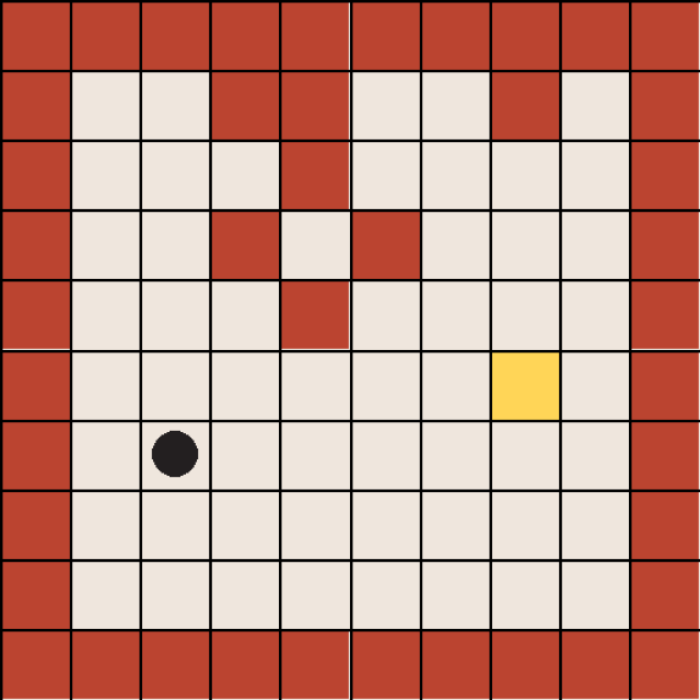
Figure 2: GridWorld, left to right: A scheme of the benchmark arena, and the average success rate and collision rate obtained during the DRL training process.

Results. We trained a pool of $500$ models, differing in the random seed used to generate them. Next, we retained only the models that demonstrated very high performance, i.e., reached our cutoff threshold of a $98\%$ success rate, with successful trajectories in over $100$ consecutive trials (see center images in Fig. 2). We also point out that even after extensive training, there was not a single model that achieved a $0\%$ collision rate (see rightmost image in Fig. 2). We note that this is in line with previous research on DRL safety, which demonstrated that even state-of-the-art agents may indeed violate simple safety requirements (?; ?; ?) — further motivating the need for shielding even in this, relatively simple, task. Next, we showcase that $S_{\mathcal{T}}$ can efficiently eliminate collisions via the usage of safety properties that cause the agent to collide in the next time-step, and overriding these, unwanted actions. For example, if the agent is near an obstacle on the left   then it should not select the next action to be LEFT. We now analyze the runtime impact of $S_{\mathcal{T}}$ on real executions of $D\cdot S_{\mathcal{T}}$. Tab. 1 present the first $10$ results, where we can see that our proposed solution successfully eliminates all possible collisions, resulting in safer behavior. Nevertheless, we point out that the increased safety did not compromise the general performance of the agent, as can be seen by the unaltered success rate.

Seed	Without Shield		With Shield		Overhead
	Succ.	Coll.	Succ.	Coll.
0	$89\%$	$3\%$	$89\%$	$0\%$	$219.1\%$
1	$92\%$	$1\%$	$93\%$	$0\%$	$182.4\%$
2	$91\%$	$2\%$	$92\%$	$0\%$	$204.6\%$
3	$91\%$	$3\%$	$91\%$	$0\%$	$240.9\%$
4	$92\%$	$2\%$	$92\%$	$0\%$	$206.5\%$
5	$89\%$	$1\%$	$90\%$	$0\%$	$213.1\%$
6	$92\%$	$2\%$	$92\%$	$0\%$	$212.1\%$
7	$86\%$	$6\%$	$91\%$	$0\%$	$250.9\%$
8	$92\%$	$1\%$	$92\%$	$0\%$	$226.2\%$
9	$89\%$	$3\%$	$91\%$	$0\%$	$220.0\%$

Table 1: A performance comparison for the agent with and without the safety shield. The values are obtained over $100$ episodes for each of the seeds.

Although $D\cdot S_{\mathcal{T}}$ completely avoids collisions, this comes at a price: $D\cdot S_{\mathcal{T}}$ checks in each time-step whether $(v_{\overline{x}},v_{\overline{y}})$ is correct with respect to $\varphi_{\mathcal{T}}$ (and overrides it if not). This, in turn, introduces a computational overhead in the execution. In the case of GW, we note that the overhead is significant (around 200%), which suggests that the choice of using a more permissive $S_{\mathcal{T}}$ (see Subsec. 3.2), might be preferable in domains where runtime optimization is essential. Note that success ratios do not necessarily increase to $100\%$ when shielded, as collision avoidance may cause some loops instead of collisions. Nevertheless success never decreases.

4.2 Temporal Dynamics

Req.	(Wu et al.)		Ours
	$\mathbb{B}$	$\mathcal{T}$	$\mathbb{B}$	$\mathbb{B}^{\prime}$	$\mathcal{T}$	$\mathcal{T}_{\mathbb{Z}}$	$\mathcal{T}_{A}$	$\mathcal{T}_{B}$
$\varphi_{0}$	$.30$	$631$	$.19$	$.17$	$171$	$173$	$183$	$184$
$\varphi_{1}$	$.41$	$590$	.22	.21	190	192	199	212
$\varphi_{2}$	$.80$	$520$	.24	.20	214	194	214	199
$\varphi_{3}$	$.45$	$340$	.22	.18	106	105	120	105
$\varphi_{4}$	$.50$	$640$	.21	.17	118	122	120	117
$\varphi_{5}$	$.80$	$520$	.21	.16	124	124	127	156
$\varphi_{6}$	$.37$	$370$	.16	.14	141	156	148	151
$\varphi_{7}$	$.49$	$710$	.20	.20	163	159	165	173
$\varphi_{8}$	$.45$	$580$	.21	.15	133	134	143	189
$\varphi_{9}$	$.18$	$610$	.14	.11	170	179	172	203
$\varphi_{10}$	$.50$	$690$	.25	.19	173	168	182	177
$\varphi_{11}$	$.31$	$530$	.21	.17	177	178	191	177
$\varphi_{12}$	$.57$	$510$	.29	.22	156	155	179	182

Table 2: Comparison of (?) and our approach (in $\mu s$)

We now show how $S_{\mathcal{T}}$ can manage both rich data and temporal dynamics. To do so, we used $13$ different specifications from (?), which are, to the best of our knowledge, the only previous successful attempt to compute rich-data shields. We generated our shield and measured time for computing: (i) the Boolean step (columns $\mathbb{B}$), and (ii) producing the final output (columns $\mathcal{T}$). We compared our results at Tab. 2. For the first task, our approach, on average, requires less than $0.21\mu{}s$, while (?) takes more than twice as long on average (with over $0.47\mu{}s$). Our approach was also more efficient in the second task, taking on average about $0.157ms$, whereas (?) required $0.557ms$ on average. Moreover, note that our ($\mathbb{B}$) contains both detection and correction of candidate outputs, whereas ($\mathbb{B}$) of  (?) only contains detection.

It is important to note another key advantage of our approach:  (?) necessarily generates a WR, whereas we can also construct $C_{\mathcal{T}}$ (column $\mathbb{B}^{\prime}$), performs considerably faster (and can operate leveraging highly matured techniques, e.g., bounded synthesis). In addition to this, we (?) presents a monolithic method that to be used with specifications containing only linear real arithmetic $\mathcal{T}_{\mathbb{Z}}$. Hence, if we slightly modify $\mathcal{T}$ to $\mathcal{T}_{\mathbb{Z}}$, then the method in (?) cannot provide an appropriate shield, whereas we do (column $\mathcal{T}_{\mathbb{Z}}$) (neither for non-linear $\mathcal{T}$). In contrast, our method encodes any arbitrary $\exists^{*}\forall^{*}$ decidable fragment of $\mathcal{T}$ (e.g., non-linear arithmetic or the array property fragment (?)). Additionally, we can optimize the outputs of $S_{\mathcal{T}}$ with respect to different criteria, such as returning the smallest/greatest safe output (column $\mathcal{T}_{A}$) and the output closest to the candidate (column $\mathcal{T}_{B}$), for which we used Z3 with OMT (?; ?). These experiments show the applicability of our approach.

5 Related Work and Conclusion

Related Work.

Classic shielding approaches (?; ?; ?; ?; ?; ?; ?) focus on properties expressed in Boolean LTL, and are incompatible for systems with richer-data domains: i.e., they need explicit manual discretization of the requirements. In the other hand, we have a sound procedure that directly takes $\textup{LTL}_{\mathcal{T}}$ specifications, which is fundamentally new. Other, more recent, work (?; ?; ?) proves that, under certain conditions, $\textup{LTL}_{\mathcal{T}}$ synthesis is decidable via abstraction methods, which can be understood as computing minterms to produce symbolic automata and transducers (?) from reactive specifications, and using antichain-based optimization, as suggested by (?). We complement and extend these techniques and demonstrate that they can act as a basis for shields synthesis modulo theories, which also contains an error detection phase whose design is essential for permissivity and which can optimize the output with respect to the erroneous candidate. Our work also includes an in-depth comparison to  (?), that present a competing method for synthesizing shields in the $\mathcal{T}$ of linear real arithmetic, which does not cover such an expressive fragment and only computes WR.

As for reactive synthesis, methods for infinite theories have also been proposed. Moreover, some of them consider a expressive temporal logics where not only multi-step properties can be defined, but also variables can convey information across-time  (?). However, they do not guarantee success (?) or termination (?; ?; ?; ?; ?), and can be unsound for some cases (?) or may need guidance (?). Therefore, any shield synthesis techniques derived from these would be incomplete. Runtime enforcement (?; ?; ?) is an additional technique similar to shielding, but it is not compatible with reactive systems (?). In addition, supervisory control of discrete event systems (?) is based on invariant specifications and controllable events, and while reactive shield-synthesis additionally admits rich temporality, supervisory control cannot be applied to temporal settings (e.g., the one presented in Subsec. 4.2).

Other approaches for ensuring DNN safety rely on formal verification (?; ?; ?; ?; ?; ?; ?; ?; ?; ?; ?; ?; ?; ?; ?; ?; ?; ?; ?; ?; ?) and Scenario-Based Programming (?; ?; ?). but they have limited scalability and expressivity.

Conclusion.

In this work, we present the first general methods for shielding properties encoded in $\textup{LTL}_{\mathcal{T}}$. These allows engineers to guarantee the safe behavior of DRL agents in complex, reactive environments. Specifically, we demonstrate how shields can be computed from a controller and from a winning region. This is not simply a direct application of synthesis, instead, we can guarantee maximally and minimally permissive shields, as well as shields optimized with respect to objective functions in arbitrary decidable $\mathcal{T}$. We also empirically demonstrate its applicability.

A next step is to adapt shields modulo theories to probabilistic settings (e.g., shielding POMDPs) (?; ?; ?; ?). Also, we plan on incorporating our shield along with complementary DNN verification engines. Another direction of future work relies on recent results for satisfiability of finite-trace $\textup{LTL}_{\mathcal{T}}$ (?), as we aim to identify fragments of $\textup{LTL}_{\mathcal{T}}$ with across-time data-transfer for which reactive synthesis is decidable. Future work may also include $\textup{LTL}_{\mathcal{T}}$ shields for multi-agent and planning scenarios (?; ?; ?; ?), and combinations with uncertainty or continuous time (?; ?; ?; ?). We want to adapt results to finite traces (?), since our agents either collide, reach the goal or have a time limit (unknown a priori).

Appendix A First-Order Theories

Due to lack of space, we have not been able to define the first-order theories extensively in Sec. 2, so we show their formalisation and details below.

Definition.

We use sorted first-order theories for extending the expressivity of the atomic predicates. For our purposes, a (sorted) first-order theory $\mathcal{T}$ consists of (1) a first-order vocabulary to form terms and predicates, (2) an interpretation of the domains of the sorts, and (3) an automatic reasoning system to decide the validity of sentences in the theory. A first-order theory $\mathcal{T}$ (see e.g., (?)) is given by its signature $\Gamma$, which is a set of constant, function, and predicate symbols. A $\Gamma$-formula is constructed from constant, function, and predicate symbols of $\Gamma$, together with logical connectives and quantifiers. The symbols $\Gamma$ are symbols without prior meaning that are later interpreted.

A $\Gamma$-formula $\varphi$ is valid in the theory $\mathcal{T}$ (i.e., $\varphi$ is $\mathcal{T}$-valid), if for every interpretation $I$ that satisfies the axioms of $\mathcal{T}$, then $I\vDash\varphi$. We write $\mathcal{T}\vDash\varphi$ to mean that $\varphi$ is $\mathcal{T}$-valid. Formally, the theory $\mathcal{T}$ consists of all closed formulae that are $\mathcal{T}$-valid, where closed means that all the variables are quantified in the formula A $\Gamma$-formula $\varphi$ is satisfiable in $\mathcal{T}$ (i.e., $\mathcal{T}$-satisfiable), if there is a $\mathcal{T}$-interpretation $I$ that satisfies $\varphi$.

A theory $\mathcal{T}$ is decidable if $\mathcal{T}\vDash\varphi$ is decidable for every $\Gamma$-formula $\varphi$. That is, there is an algorithm that always terminates with $\top$ if $\varphi$ is $\mathcal{T}$-valid or with $\perp$ if $\varphi$ is $\mathcal{T}$-invalid.

Arithmetic theories

A particular class of first-order theories is that of arithmetic theories, which are well studied in mathematics and theoretical computer science, and are of particular relevance in formal methods. Most of these theories are decidable. In this paper, we use three of them:

• Linear Integer Arithmetic $\mathcal{T}_{\mathbb{Z}}$ the theory of integer numbers with addition but no arbitrary multiplication The signature is $\Gamma_{\mathbb{Z}}=\{\ldots,-1,0,1,\ldots,,+,-,=,>\}$. An example of a literal is $(2x>-4)$.

• Linear Rational/Real Arithmetic $\mathcal{T}_{\mathbb{Q}}$: the theory of real/rational numbers with addition but no arbitrary multiplication The signature is $\Gamma_{\mathbb{Q}}=\{0,k,+,-,=,>\}$, where $k\in\mathbb{Q}$. For instance, a literal is $(2x>-\frac{1}{3})$.

• Nonlinear Real Arithmetic $\mathcal{T}_{\mathbb{R}}$ is the theory of real numbers with both addition and arbitrary multiplication The signature is $\Gamma_{\mathbb{R}}=\{0,k,+,-,=,>,\cdot\}$. An example of a literal is $(2x^{2}>\frac{1}{3})$.

Note that a theory of (linear) naturals $\mathcal{T}_{\mathbb{N}}$ is subsumed by $\mathcal{T}_{\mathbb{Z}}$ and a theory of (non-linear) complex numbers is subsumed by $\mathcal{T}_{\mathbb{C}}$.

Fragments of $\mathcal{T}$.

A fragment of a theory is a syntactically-restricted subset of formulae of the theory. For example, the quantifier-free fragment of a theory $\mathcal{T}$ is the set of formulae without quantifiers that are valid in $\mathcal{T}$. A fragment of $\mathcal{T}$ is decidable if $\mathcal{T}\vDash\varphi$ is decidable for every $\Gamma$-formula $\varphi$ in the fragment.

In this paper, we considered theories $\mathcal{T}$ whose $\exists^{*}\forall^{*}$ fragment is decidable, which not only considers arithmetic theories, but many others such as, the array property fragment (?), which is decidable for the $\exists^{*}\forall_{\mathbb{Z}}$ fragment. Indeed, many others theories beyond numerical domains span from Bernays–Schönfinkel–Ramsey (BSR) class (?), which is less expressive than the general $\exists^{*}\forall^{*}$-fragment considered in this paper. For instance, (?) shows decidability of the fragment of first-order separation logic (SL) restricted to BSR where the quantified variables range over the set of memory location; however, SL becomes undecidable when the quantifier prefix belongs to $\exists^{*}\forall^{*}\exists^{*}$.

Appendix B Deep Neural Networks and Verification

B.1 Deep Neural Networks (DNNs)

A DNN (?) is a directed, computational graph, consisting of a sequence of layers. The DNN is evaluated by propagating its input values, layer-by-layer, until reaching the final (output) layer. The computed output values can be interpreted as a regression value, or a classification, depending on the type of the DNN in question. The computation itself depends also on the type of the DNN’s layers. For example, a node $z$ in a rectified linear unit (ReLU) layer calculates the value $z=\text{ReLU}{}(x)=\max(x,0)$, for the value $x$ of one of the nodes among the preceding layers. Other layer types include weighted sum layers (that compute an affine transformation), and various layers with non-linear activations. As in most prior work on DNN verification, we focus on DNNs in which every layer is connected exclusively to its following layer; these general architectures are termed feed-forward neural networks, and are extremely popular. A toy (regression) DNN is depicted in Fig. 3. For an input vector $V_{1}=[1,2]^{T}$, the values $V_{2}=[10,-5]^{T}$ are computed by the second layer. Subsequently, in the third layer, ReLU activations are applied, producing the vector $V_{3}=[10,0]^{T}$. Finally, the single output value of the network is $V_{4}=[10]$.

Figure 3: A toy DNN.

B.2 Deep Reinforcement Learning

In this paper, we focus on Deep Reinforcement Learning (DRL) (?; ?), which is a popular paradigm in the unsupervised learning setting, for training DNNs, in which the DNN agent learns from experience, instead of data. Specifically, the agent is iteratively trained to learn a policy $\pi$, mapping every environment state $s$ (observed by the agent) to an appropriate action $a$. The learnt policy has various interpretations across different training algorithms (?; ?; ?). For example, in some cases, $\pi$ may represent a probability distribution over the possible actions, while in other cases it may encode a function estimating a desirability metric over all future actions from a given state $s$. DRL agents are pervasive among various safety-critical domains, and especially, among robotic systems (?; ?; ?; ?).

B.3 DNN Verification

A DNN verification engine (?; ?; ?; ?; ?; ?) receives as inputs: a DNN $N$, a precondition $P$ over the network’s inputs, and a postcondition $Q$ limiting the network’s outputs. The verification engine searches for an input $y$ satisfying the property $P(y)\wedge Q(N(y))$. If there exists such an input, a SAT result is returned, along with a concrete input $z$ satisfying the constraints; otherwise, UNSAT is returned, indicating that no such input exists. Typically, the postcondition $Q$ specifies the negation of the desired property, and thus a SAT results implies that the property is violated, with the returned $z$ being an input that triggers a bug. However, an UNSAT result implies that the (desired) property holds throughout the input space.

Marabou. In this work, the DNN verification procedure was executed by Marabou (?), a popular verification engine that has achieved state-of-the-art results on a wide variety of DNN benchmarks (?; ?).

Example. For instance, if we were to check whether the DNN depicted in Fig. 3 always outputs a value larger than $7$; i.e., for any input $x=\langle v_{1}^{1},v_{1}^{2}\rangle$, then $N(x)=v_{4}^{1}>7$. This property can be encoded as a verification query with a precondition that does not restrict the inputs, i.e., $P=(true)$, and by setting the postcondition $Q=(v_{4}^{1}\leq 7)$. For this query, a sound verification engine will return a SAT answer, alongside a feasible counterexample, e.g., $x=\langle 2,0\rangle$, which produces $v_{4}^{1}=7\leq 7$, proving that this property does not hold for the DNN in question.

Complexity. It has been shown that the process of sound and complete verification of a given DNN with ReLU activations is ‘NP-complete. Hence, even a linear growth to the size of a DNN (i.e., the total number of weights and neurons) can cause in the worst-case scenario, an exponential blowup in verification runtime. This complexity was deduced by Katz et al. (?), by presenting a polynomial-time reduction from the popular 3-SAT problem, known to be NP-complete. We note however, that there exist various heuristics that allow to efficiently prune the search space and reduce the overall verification time in many cases (?; ?).

B.4 Comparing Shielding with DNN Verification

DNN verification is the classic alternative approach to shielding. In the DNN verification setting, we train a collection of models, and check independently whether each model obeys all required properties. After the verification process, we hope to retain a model that will behave correctly.

General Comparison.

Next, we will cover the main advantages and setback on using each of these two competing approaches:

1. Activation Functions and Model Expressivity. Marabou and most DNN verification engines can verify only piecewise-linear constraint. Hence, this significantly limits the type of DNN being verified, as well as the property in question. Shields, on the other hand, tree to DNN as a black box input/output system, and are agnostic to the expressivity level of the DNN in question. In addition, our shielding approach is limited solely to the expressivity of arbitrary LTL formulas.

2. Verification Runtime. Another advantage of shields is that they are significantly faster to implement when compared to DNN verification. This for two reasons. First, a single shield can be used for all DRL agents and all properties, while an SMT-based verification engine, for example, must verify each property separately, per each separate agent. To demonstrate this point, we verified $7$ properties per each of the $700$ DRL agents trained on the TurtleBot benchmark. This resulted in $4,900$ unique verification queries (one per each DRL agent, and per each property). In addition to verification finding violations (i.e., SAT assignments) for all properties, the accumulative runtime with Marabou was over $1,935$ seconds (!), when running also with a state-of-the-art Gurobi solver (?). These results are depicted in Fig. 4.

3. Pervasiveness. On the other hand, a clear advantage of DNN verification, relative to shielding, is that DNN verification can be executed offline. Thus, given that DNN verification identifies a correct model, it can be deployed safely into the wild, without and pervasive intervention of additional sources. Shielding on the other hand, constantly requires monitoring of the decisions of a given DRL system.

4. System Soundness. Finally, we note that given a DNN verification engine identifies a successful agent, we can rely with high confidence on the, original, decided actions — otherwise, an incorrect action that would have violated a property, should be identified beforehand with verification. Shielding, on the other hand, constantly requires overriding the unwanted behavior, and hence possibly enforcing an action that can be sub-optimal.

Note. It is still worth mentioning that there are no formal guarantees that a single DNN agent will indeed “survive” the formal-verification-driven filtering process. For example, in all $4,900$ verification queries described in Fig. 4, all $700$ agents were found to violate all properties, at least in a single scenario. We believe that these empirical results further motivate the need for shielding.

Figure 4: Total accumulated time (in log-scale) for all 4,900 experiments, all of which include violations of the properties of interest.

Complexity Comparison.

As the complexity of our shielding approach is dominated by the complexity of LTL synthesis, it is 2EXPTime-complete in general. In practice, however, many LTL fragments tend to be synthesized in a runtime process that is significantly more efficient than this worst-case complexity; e.g., GR(1), GX0, etc. But most importantly, the NP-completeness is not on the same measure of size (i.e., total neurons of the DNN) than the LTL formula, which is significantly smaller, in practice. DNN verification on the other hand, is NP-complete (?), as a function of the size of the DNN in question, i.e., the total number of DNN parameters. We note that a direct comparison between complexities of shielding and DNN verification is not straightforward, as each depends on a different type of input (size of the LTL formula vs. the total number of DNN parameters).

Appendix C Details about the GridWorld case study

Properties.

Specifically, we classified the wanted behaviours into two categories:

• Safety: decisions that cause the agent to collide in the next time-step. For example, when the agent is near an obstacle on the left, then it should not select the action LEFT. These properties show that, given all the necessary properties, we can avoid collision in all executions.

• Liveness: decisions that do not cause the robotic to collide in the next time-step but generate an infinite loop. For example, when the robot iteratively performs a sequence of actions that brings it to the same position (e.g., RIGHT, LEFT, and RIGHT. These properties show that our shields can manage dynamics.

Note that, although these requirements can look straightforward to accomplish for a state-of-the-art $D$, the random noise can potentially generate really specific input configuration, known as adversarial inputs, that can easily fool the neural network to perform unexpected and unexplainable actions (?).

DRL and Training Results

GridWorld is a classical problem for reinforcement learning, and many previous works efficiently solve it with many state-of-the-art solutions and algorithms. However, our modified version with the addition of a random noise to the agent readings, makes the task drastically more challenging. We design a neural network to match the state and observation space of the environment and employ a simple neural feed-forward neural network, consisting of $layers$ of $32$ neurons each, activated with the popular ReLU function. In more detail:

1. An input layer of $8$ neurons. The first $2$ inputs represent the coordinates of the agent in the grid, these inputs can assume continuous values given the addition of the Gaussian noise. The next $4$ neurons represent a proximity sensor that indicates whether the agent has an obstacle in one of the $4$ possible directions. The last $2$ input feature encodes the coordinates of the target.

2. An output layer of $4$ neurons, one for each direction (i.e., UP, LEFT, RIGHT, and DOWN). The agent always performs the action corresponding to the output node with the highest value.

We trained our agents with the state-of-the-art Proximal Policy Optimization (PPO) algorithm (?), which has shown promising results in a large variety of tasks. A crucial component of effective training is the reward function. For this task, we employ a discrete reward function, in detail:

$$r_{t}=\begin{cases}1&\text{if the target is reached}\\ -5&\text{if the agent collides}\\ -0.01&\text{otherwise}\end{cases}$$ (1)

notice that we employ a small penalty of $-0.01$ for each time step to push the agent toward finding the shortest path.

Appendix D A TurtleBot case study

Figure 5: The Clearpath Turtlebot 4 platform.

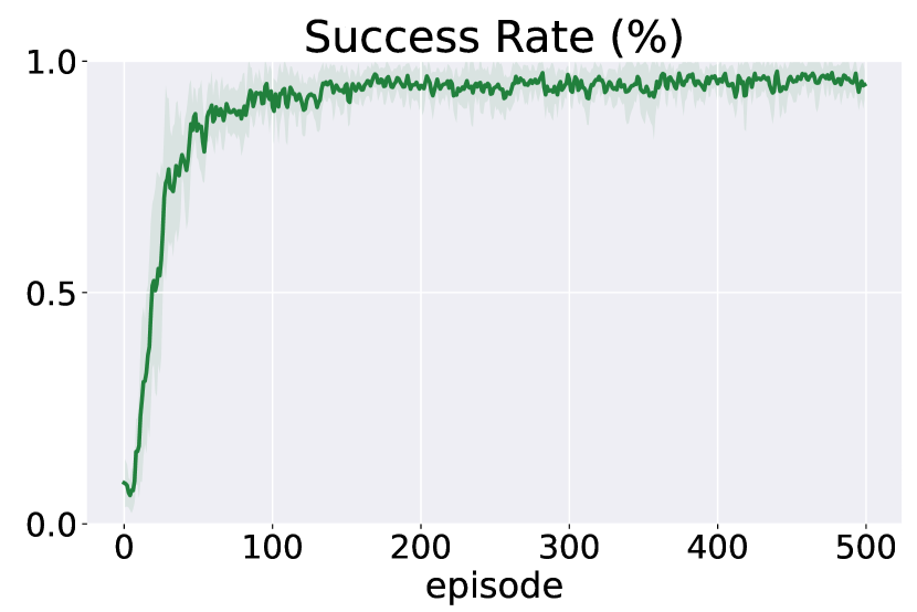
Figure 6: The average success rate obtained by our DRL-trained agents.

D.1 Expressivity in $\mathcal{T}$

Case Study: Robotic Navigation Systems. Clearpath Turtlebot 4 (TB), depicted in Fig. 6, is a widely adopted platform in the field of robotics research (?; ?; ?), given its versatility and applicability to real-world systems. Specifically, we focus on the mapless navigation variant, in which the robot (controlled by a DRL agent) learns to navigate throughout an unknown arena, relying on its lidars and other, local sensors (?; ?). For more details, see App. D.

Partial Observability. We continue to focus on collision avoidance properties. However, unlike the case with GW (Subsec. 4.1 the current environment is only partially observable. More formally, when using $S_{\mathcal{T}}$ we do not possess a complete transition model of both players. Hence, $S_{\mathcal{T}}$ can only guarantee $\varphi_{\mathcal{T}}$, but not high-level behavioural properties, e.g., collision avoidance. However, TB demonstrates that our approach allows encoding complex properties also in this harder and realistic setting. This is possible due to Thm. 1, which implies that $S_{\mathcal{T}}$ enforces $\varphi_{\mathcal{T}}$ based on many theories $\mathcal{T}$, including non-linear real arithmetic.

Empirical Evaluation. We trained a pool of $700$ models, differing in the random seed used to generate them. The models reached a high success threshold of $98\%$ (see Fig. 6). For additional details regarding the training procedure, see App. D.3. Although these models attained a high success rate; when simulated, we identified various edge cases in which they behaved unsafely. We note that these unwanted behaviors appeared even after additional, extensive training rounds. To further demonstrate our shield, we employed it to guarantee various types of wanted behavior of TB, under user-defined specifications:

• Safe: actions that do not cause the robot to collide in the next time-step. For example, when the robot is near an obstacle, then it should not move towards it.

• Predictable: actions that do not result to potentially unexpected outcomes. For example, the agent should avoid rapidly and simultaneously increasing both its angular velocity and its linear velocity.

• Efficient: actions that are optimal under the given circumstances.
  For example, if the target can be safely reached in very few time-steps, the agent should avoid unnecessarily long trajectories.

We encoded violations of five different types of safety properties (S1, S2, S3, S4, and S5), two types of violations for predictable behaviors (P1 and P2), and a violation of a single type of required efficient behavior (E1). Concretely, $D\cdot S_{\mathcal{T}}$ will output values in non-linear real arithmetic; e.g., S5 is $\neg[(x_{4}-0.17<y_{0}\cdot 0.015)\wedge(y_{1}>0.15)]$, etc. A full encoding of all properties appears in App. D.4.

Results. To analyze our approach, we randomly sampled $1000$ trajectories with various actions (some ending with a collision, and some reaching the target safely). Next, we constructed $S_{\mathcal{T}}$ to guarantee the following property combinations: spe (safe, predictable, and efficient), sp (safe and predictable), se (safe and efficient), and s (safe). Our experiments demonstrated that $S_{\mathcal{T}}$ synthesis was indeed able to detect unrealizable specifications. Also, when the specification was realizable, the synthesis runtime was extremely fast — with all shields generated in less than $7.81$ seconds.

Next, we randomly selected $10$ traces (half successful, and half not), and conducted an in-depth analysis of the behavior of our $S_{\mathcal{T}}$ — both in terms of runtime, and in terms of overriding actions. Specifically, we aim to (1) show non-linear outputs and (2) understand how the combinations of various properties can affect runtime and corrections. Our results are summarized in Tab. 3, and include, per each trace (row) and property combination (column), the mean execution time (Tm.) for generating $S_{\mathcal{T}}$, as well as the ratio of overwritten actions (O), out of all actions in total (T). First, we analyzed how the addition of properties affects the overall behavior of the shield. Indeed, the results behaved as expected — the more properties that were enforced (s$\rightarrow$ sp,se$\rightarrow$spe) the less permissive $S_{\mathcal{T}}$ was, i.e., the higher the O/T ratio was, as there were more “wrong” behaviors to correct. Another observed behavior is that, in most cases, the more properties that $\varphi_{\mathcal{T}}$ encoded, the more time it took for $S_{\mathcal{T}}$ to override actions. This too, was not surprising, as more properties are translated to more constraints considered by the underlying SMT solver. Our analysis also raised some surprising results. For example, by comparing property combinations sp and se, it is evident that there is a vast difference between the success in learning various properties. For example, the shields tend to intervene significantly more when enforcing “predictable” behavior, than when enforcing “efficent” behavior. The fact that “efficient” decisions are corrected much less (especially in failure traces) suggests that these behaviors are learned more successfully during training. This also demonstrates how shielding can be used not only for guaranteeing correctness, but for understanding the generalization of these “black box” DRL artifacts. Also, we can observe overall a considerable amount of actions overridden by $S_{\mathcal{T}}$ in almost all experiments, even though the robot is controlled by highly-successful DRL agents. We believe that this further demonstrates the merits of our approach. For additional details, see App. D.

Trace	spe			sp			se			s
	Tm.	O/T	%	Tm.	O/T	%	Tm.	O/T	%	Tm.	O/T	%
$00.00$	$64$	$172/288$	$59.7$	$59$	$77/288$	$26.7$	$61$	$142/288$	$49.3$	$57$	$47/288$	$16.3$
$00.06$	$60$	$86/225$	$38.2$	$60$	$62/225$	$27.5$	$58$	$75/225$	$33.3$	$57$	$51/225$	$22.6$
$00.08$	$64$	$109/268$	$40.6$	$61$	$101/268$	$37.6$	$59$	$65/268$	$24.2$	$57$	$57/268$	$21.2$
$01.01$	$66$	$119/206$	$57.7$	$61$	$96/206$	$46.6$	$59$	$70/206$	$33.9$	$57$	$47/206$	$22.8$
$01.02$	$64$	$133/342$	$38.8$	$62$	$129/342$	$37.7$	$63$	$56/342$	$16.3$	$52$	$52/342$	$15.2$
$00.07$	$76$	$21/21$	$100.0$	$74$	$21/21$	$100.0$	$72$	$21/21$	$100.0$	$71$	$21/21$	$100.0$
$13.07$	$70$	$29/54$	$53.7$	$68$	$29/54$	$53.7$	$67$	$13/54$	$24$	$67$	$13/54$	$24$
$29.02$	$73$	$7/9$	$77.7$	$72$	$7/9$	$77.7$	$66$	$2/7$	$28.5$	$64$	$2/7$	$28.5$
$48.05$	$63$	$70/372$	$18.8$	$62$	$70/372$	$18.8$	$59$	$34/372$	$9.1$	$61$	$34/372$	$9.1$
$59.07$	$68$	$15/51$	$29.4$	$69$	$15/51$	$29.4$	$63$	$7/51$	$13.7$	$67$	$7/51$	$13.7$

Table 3: For each trace and property combination, we present the average $S_{\mathcal{T}}$ intervention time and number of corrections (first $5$ traces are successful, and the last $5$ traces are not). Time is measured in milliseconds.

D.2 DRL and Training Results

State-of-the-art solutions suggest that it is possible to train an effective agent by exploiting simple neural architecture. In particular, we took inspiration from the topology presented in previous related work (?; ?) that consists of a modest feed-forward DRL, consisting of two hidden layers of $32$ neurons each, with the popular ReLU activation units. As our DRL is a regression (and not a classification) network, we were able to directly encode continuous actions in the output layer, hence allowing the DRL agents to potentially encode any possible action in the state space. More formally, we summarize the network’s topology as follows:

1. An input layer of $9$ neurons. The first 7 inputs represent lidar sensor readings, that indicate the distance from an obstacle in a given direction (from left to right, with a step of $30^{\circ}$); the last two input nodes represent the local position of the target in polar coordinates (i.e., angle and distance).

2. Two fully connected hidden layers of $32$ neurons, with ReLU activations.

3. An output layer of $2$ neurons. The first neuron returns the linear velocity (i.e., the speed of the robot), and the second one provides the angular velocity (i.e., a single value indicating the rotation). These two values together allow to directly evaluate the location of the robot in the next time step.

We trained our agents with the state-of-the-art Proximal Policy Optimization (PPO) algorithm (?), which has shown promising results in a large variety of tasks, specifically, in robotics navigation. A crucial component of effective training is the reward function. In this work, we exploited a continuous reward, with the addition of discrete bonuses to encourage (or discourage) specific behaviors. More formally, the reward ($R_{t}$) during time-step $t$ of the training phase is defined as follows:

$$R_{t} =\begin{cases}\pm 1&\text{terminal states}\\ (dist_{t-1}-dist_{t})\cdot\eta-\beta&\text{otherwise}\end{cases}$$ (2)

Where $dist_{k}$ is the distance from the target at time $k$; $\eta$ is a normalization factor; and $\beta$ is a penalty, designed to encourage the robot to reach the target quickly (in our experiments, we empirically set $\eta=3$ and $\beta=0.001$). Additionally, in terminal states, we increase the reward by $1$ if the target is reached, or decrease it by $1$ in case of collision.

D.3 Training Details

Now we discuss the hyperparameters for training and various implementation details for TurtleBot.

General Parameters

• training episodes: 500

• number of hidden layers: 2

• size of hidden layers: 32

• parallel environments: 1

• gamma ($\gamma$): 0.99

• learning rate: $0.0003$

We followed the insights from (?) for the network topology (see Sec.D.1 of the main paper). However, a crucial difference, between our setting and the one appearing in (?), is that our agents have two continuous outputs, instead of five discrete possible actions; this provides our agent with a higher expressiveness level.

PPO Parameters For the advantage estimation and the critic update, we rely on the generalized advantage estimation strategy (GAE). The update rule follows the guidelines of the OpenAI’s Spinning Up documentation. Following is a complete list of the hyperparameters for our training:

• memory limit: None

• update frequency: 4096 steps

• trajectory reduction strategy: sum

• actor epochs: 50

• actor batch numbers: 16

• critic epochs: 60

• critic batch numbers: 32

• critic network size: 2x256

• PPO clip: 0.2

• GAE lambda: 0.95

• target kl-divergence: 0.02

• max gradient normal: 0.5

Random Seeds for Reproducibility: finally, we present a complete list of the random seeds we used for the training: [$84$, $234$, $256$, $403$, $597$, $634$, $732$]. These seeds are applied to the following Python modules: Random, NumPy, and PyTorch. We plan on making our experiments publicly available in the final version of this paper.

D.4 Requirements Formalization

The first $7$ inputs of the network (i.e., the lidar scans) are normalized in the range $[0,1]$, where $0$ means that the obstacle is at the minimum distance and $1$ means that the path is free in the required direction; the input number $8$ (i.e., distance from the target) is normalized between $0$ and $1$ on the size of the map; finally, the last input (i.e., the angle for the polar coordinates) is normalized between $0$ (target on the left) and $1$ (target on the right).

However, given the following consideration, we found that these standard bounds can be further tightened: (i) the true lower-bound for a lidar scan can be increased to a value of $0.03$ to guarantee a minimal room for rotating the robot; (ii) the proportion between the distance from an obstacle and the maximum linear velocity that allows a safe collision avoidance is a factor $\alpha=0.015$ (the following encoding shows the effect of this parameter); and (ii) to avoid configurations in which the agent can solve the task in less than $3$ steps, we set a minimum distance from the target of $0.2$.

Complete list of constraints and requirements: notice that all the following properties are encoded as unwanted behaviors, i.e., something that the agent should NOT do. Notice that with $X$ we represent the input nodes and with $Y$ the outputs.

• SAFETY 1 (S1): avoid collision with an obstacle in front of the robot.

  • $X[3]-0.17<Y[0]\cdot 0.015$

• SAFETY 2 (S2): avoid collision with an obstacle on the left of the robot.

  • ($X[1]-0.17<Y[0]\cdot 0.015$) and ($Y[1]<-0.2$)

• SAFETY 3 (S3): avoid collision with an obstacle slightly on the left of the robot.

  • ($X[2]-0.17<Y[0]\cdot 0.015$) and ($Y[1]<-0.15$)

• SAFETY 4 (S4): avoid collision with an obstacle on the right of the robot.

  • ($X[5]-0.17<Y[0]\cdot 0.015$) and ($Y[1]>0.2$)

• SAFETY 5 (S5): avoid collision with an obstacle slightly on the right of the robot.

  • ($X[4]-0.17<Y[0]\cdot 0.015$) and ($Y[1]>0.15$)

• PREDICTABLE 1 (P1): avoiding a strong rotation if the robot is accelerating.

  • $Y[1]>3\cdot Y[0]^{2}$

• PREDICTABLE 2 (P2): avoiding a strong acceleration while the robot is rotating.

  • $abs(Y[1])>0.7$ and $Y[0]>0.7$

• EFFICIENT 1 (E1): avoid turning if the goal is in front of the robot and there are no obstacles in that direction.

  • $X[1]>0.45$ and $X[7]<0.55$ and $X[3]==1$ and $Y[1]>0.05$

D.5 Evaluation: Component-level Runtime Analysis.

Moreover, we checked in a higher resolution which of the shield’s components are the most resource-consuming. We selected another collection of $20$ traces, for which we measured the synthesis time of the underlying components: partitioner (Pa.), Boolean controller (Cn.) and provider (Pr.). The results (summarized in Tab. 4) suggest that the partitioner is the component that takes the most time (about $0.04$ seconds). This is probably due to the current partitioner implementation which relies on an exhaustive exhaustive algorithm to do so. We acknowledge that the implementation of Pa. and Pr. is made in Python, whereas Cn. is an external component aigsim in C, so shield performance would benefit from any advance in such implementations. Note that the amount of intervention of the shield is high because we are considering safety, dangerous, and behavioral properties. Also, note that this amount is usually higher than $80\%$ when the trace represents a trajectory in which the agent failed to reach the target.

Trace	Component times			Overall measures
	Pa.	Cn.	Pr.	Ex.	O/T	%
$00$	$0.019$	$1.187(5)$	$0.016$	$3.160$	$13/88$	$14.77$
$01$	$0.041$	$1.943(6)$	$0.019$	$29.038$	$334/478$	$69.87$
$02$	$0.041$	$4.213(6)$	$0.017$	$22.397$	$186/379$	$49.07$
$03$	$0.043$	$4.251(6)$	$0.018$	$22.659$	$289/367$	$78.74$
$04$	$0.038$	$3.573(6)$	$0.018$	$11.851$	$149/207$	$71.98$
$05\times$	$0.049$	$1.299(5)$	$0.017$	$8.659$	$112/128$	$87.50$
$06\times$	$0.050$	$5.613(6)$	$0.018$	$8.261$	$107/119$	$89.91$
$07\times$	$0.048$	$1.783(6)$	$0.017$	$29.420$	$200/448$	$44.64$
$08$	$0.033$	$6.460(6)$	$0.017$	$7.392$	$78/143$	$54.54$
$09$	$0.017$	$1.017(5)$	$0.015$	$2.806$	$0/82$	$0.00$
$10$	$0.042$	$4.251(6)$	$0.017$	$19.641$	$150/330$	$45.45$
$11\times$	$0.049$	$2.690(5)$	$0.018$	$19.641$	$49/49$	$100.00$
$12$	$0.039$	$3.193(6)$	$0.017$	$13.472$	$139/233$	$59.65$
$13\times$	$0.033$	$3.648(6)$	$0.018$	$14.556$	$225/279$	$80.65$
$14$	$0.040$	$3.785(6)$	$0.016$	$14.866$	$90/260$	$34.61$
$15$	$0.040$	$5.678(6)$	$0.017$	$16.513$	$221/283$	$78.09$
$16\times$	$0.042$	$2.478(6)$	$0.018$	$14.556$	$415/606$	$68.48$
$17$	$0.044$	$5.238(6)$	$0.018$	$32.910$	$288/522$	$55.17$
$18$	$0.018$	$6.568(6)$	$0.015$	$3.465$	$0/100$	$0.00$
$19\times$	$0.050$	$8.744(6)$	$0.018$	$5.981$	$87/87$	$100.00$

Table 4: Time-wise performance of components. “X” in the first columns indicates the trace represents a failed trajectory. (Ex.) measures the execution time for the whole trace.

References

- Alshiekh et al. 2018 Alshiekh, M.; Bloem, R.; Ehlers, R.; Könighofer, B.; Niekum, S.; and Topcu, U. 2018. Safe Reinforcement Learning via Shielding. In Proc. of the 32nd AAAI Conference on Artificial Intelligence, 2669–2678.
- Amir et al. 2021 Amir, G.; Wu, H.; Barrett, C.; and Katz, G. 2021. An SMT-Based Approach for Verifying Binarized Neural Networks. In Proc. 27th Int. Conf. on Tools and Algorithms for the Construction and Analysis of Systems (TACAS), 203–222.
- Amir et al. 2022 Amir, G.; Zelazny, T.; Katz, G.; and Schapira, M. 2022. Verification-Aided Deep Ensemble Selection. In Proc. 22nd Int. Conf. on Formal Methods in Computer-Aided Design (FMCAD), 27–37.
- Amir et al. 2023a Amir, G.; Corsi, D.; Yerushalmi, R.; Marzari, L.; Harel, D.; Farinelli, A.; and Katz, G. 2023a. Verifying Learning-Based Robotic Navigation Systems. In Proc. 29th Int. Conf. on Tools and Algorithms for the Construction and Analysis of Systems (TACAS), 607–627.
- Amir et al. 2023b Amir, G.; Freund, Z.; Katz, G.; Mandelbaum, E.; and Refaeli, I. 2023b. veriFIRE: Verifying an Industrial, Learning-Based Wildfire Detection System. In Proc. 25th Int. Symposium on Formal Methods (FM), 648–656.
- Amir et al. 2023c Amir, G.; Maayan, O.; Zelazny, T.; Katz, G.; and Schapira, M. 2023c. Verifying Generalization in Deep Learning. In Proc. 35th Int. Conf. on Computer Aided Verification (CAV), 438–455.
- Amir, Schapira, and Katz 2021 Amir, G.; Schapira, M.; and Katz, G. 2021. Towards Scalable Verification of Deep Reinforcement Learning. In Proc. 21st Int. Conf. on Formal Methods in Computer-Aided Design (FMCAD), 193–203.
- Ashok et al. 2020 Ashok, P.; Hashemi, V.; Kretinsky, J.; and Mühlberger, S. 2020. DeepAbstract: Neural Network Abstraction for Accelerating Verification. In Proc. 18th Int. Symposium on Automated Technology for Verification and Analysis (ATVA).
- Avni et al. 2019 Avni, G.; Bloem, R.; Chatterjee, K.; Henzinger, T. A.; Könighofer, B.; and Pranger, S. 2019. Run-time optimization for learned controllers through quantitative games. In Proc. of the 31st International Conference in Computer Aided Verification (CAV), Part I, volume 11561 of LNCS, 630–649. Springer.
- Bassan and Katz 2023 Bassan, S., and Katz, G. 2023. Towards Formal Approximated Minimal Explanations of Neural Networks. In Proc. 29th Int. Conf. on Tools and Algorithms for the Construction and Analysis of Systems (TACAS), 187–207.
- Bassan et al. 2023 Bassan, S.; Amir, G.; Corsi, D.; Refaeli, I.; and Katz, G. 2023. Formally Explaining Neural Networks within Reactive Systems. In Proc. 23rd Int. Conf. on Formal Methods in Computer-Aided Design (FMCAD), 10–22.
- Bernreiter, Maly, and Woltran 2021 Bernreiter, M.; Maly, J.; and Woltran, S. 2021. Choice Logics and Their Computational Properties. In Proc. of the 30th Int. Joint Conf. on Artificial Intelligence, (IJCAI 2021), 1794–1800.
- Bharadwaj et al. 2019 Bharadwaj, S.; Bloem, R.; Dimitrova, R.; Könighofer, B.; and Topcu, U. 2019. Synthesis of minimum-cost shields for multi-agent systems. In 2019 American Control Conference, ACC 2019, Philadelphia, PA, USA, July 10-12, 2019, 1048–1055. IEEE.
- Bjørner and A. 2014 Bjørner, N., and A., P. 2014. Z - Maximal Satisfaction with Z3. In Proc. of the 6th Int. Symposium on Symbolic Computation in Software Science, (SCSS), volume 30, 1–9.
- Bjørner, Phan, and Fleckenstein 2015 Bjørner, N.; Phan, A.; and Fleckenstein, L. 2015. Z - An Optimizing SMT Solver. In Proc. of the 21st Int. Conf. on Tools and Algorithms for the Construction and Analysis of Systems (TACAS), volume 9035, 194–199.
- Bloem et al. 2015 Bloem, R.; Könighofer, B.; Könighofer, R.; and Wang, C. 2015. Shield Synthesis: - Runtime Enforcement for Reactive Systems. In Proc. of the 21st Int. Conf. in Tools and Algorithms for the Construction and Analysis of Systems, (TACAS), volume 9035, 533–548.
- Bradley and Manna 2007 Bradley, A. R., and Manna, Z. 2007. The calculus of computation - decision procedures with applications to verification. Springer.
- Bradley, Manna, and Sipma 2006 Bradley, A.; Manna, Z.; and Sipma, H. 2006. What’s Decidable About Arrays? In Proc. of the 7th Int. Conf. on Verification, Model Checking, and Abstract Interpretation (VMCAI), 427–442.
- Brenguier et al. 2014 Brenguier, R.; Pérez, G. A.; Raskin, J.; and Sankur, O. 2014. Abssynthe: abstract synthesis from succinct safety specifications. In Proc. of the 3rd Workshop on Synthesis, (SYNT 2014), volume 157 of EPTCS, 100–116.
- Bunel et al. 2018 Bunel, R.; Turkaslan, I.; Torr, P.; Kohli, P.; and Mudigonda, P. 2018. A Unified View of Piecewise Linear Neural Network Verification. In Proc. 32nd Conf. on Neural Information Processing Systems (NeurIPS), 4795–4804.
- Camacho, Bienvenu, and McIlraith 2019 Camacho, A.; Bienvenu, M.; and McIlraith, S. A. 2019. Towards a unified view of AI planning and reactive synthesis. In Proc. of the 29th International Conference on Automated Planning and Scheduling (ICAPS 2019), 58–67. AAAI Press.
- Carr et al. 2022 Carr, S.; Jansen, N.; Junges, S.; and Topcu, U. 2022. Safe reinforcement learning via shielding for pomdps. CoRR abs/2204.00755.
- Carr et al. 2023 Carr, S.; Jansen, N.; Junges, S.; and Topcu, U. 2023. Safe reinforcement learning via shielding under partial observability. In Proc. of the 37th Conference on Artificial Intelligence (AAAI 2023), 14748–14756. AAAI Press.
- Carreno et al. 2022 Carreno, Y.; Ng, J. H. A.; Petillot, Y. R.; and Petrick, R. P. A. 2022. Planning, execution, and adaptation for multi-robot systems using probabilistic and temporal planning. In Proc. of the 21st International Conference on Autonomous Agents and Multiagent (AAMAS 2022), 217–225. International Foundation for Autonomous Agents and Multiagent Systems (IFAAMAS).
- Casadio et al. 2022 Casadio, M.; Komendantskaya, E.; Daggitt, M.; Kokke, W.; Katz, G.; Amir, G.; and Refaeli, I. 2022. Neural Network Robustness as a Verification Property: A Principled Case Study. In Proc. 34th Int. Conf. on Computer Aided Verification (CAV), 219–231.
- Cassandras and Lafortune 1999 Cassandras, C. G., and Lafortune, S. 1999. Introduction to Discrete Event Systems, volume 11 of The Kluwer International Series on Discrete Event Dynamic Systems. Springer.
- Choi et al. 2022 Choi, W.; Finkbeiner, B.; Piskac, R.; and Santolucito, M. 2022. Can Reactive Synthesis and Syntax-Guided Synthesis be Friends? In Proc. of the 43rd ACM SIGPLAN Int. Conf. on Programming Language Design and Implementation (PLDI), 229–243.
- Córdoba et al. 2023 Córdoba, F. C.; Palmisano, A.; Fränzle, M.; Bloem, R.; and Könighofer, B. 2023. Safety shielding under delayed observation. In Proc. of the 33th International Conference on Automated Planning and Scheduling (ICAPS’23), 80–85. AAAI Press.
- Corsi et al. 2022 Corsi, D.; Yerushalmi, R.; Amir, G.; Farinelli, A.; Harel, D.; and Katz, G. 2022. Constrained Reinforcement Learning for Robotics via Scenario-Based Programming. Technical Report. https://arxiv.org/abs/2206.09603.
- Corsi et al. 2024 Corsi, D.; Amir, G.; Katz, G.; and Farinelli, A. 2024. Analyzing Adversarial Inputs in Deep Reinforcement Learning. Technical Report. https://arxiv.org/abs/2402.05284.
- Corsi, Marchesini, and Farinelli 2021 Corsi, D.; Marchesini, E.; and Farinelli, A. 2021. Formal verification of neural networks for safety-critical tasks in deep reinforcement learning. In Uncertainty in Artificial Intelligence.
- D’Antoni and Veanes 2017 D’Antoni, L., and Veanes, M. 2017. The power of symbolic automata and transducers. In Proc. of the 29th International Conference in Computer Aided Verification (CAV 2017), Part I, volume 10426 of LNCS, 47–67. Springer.
- de Moura and Bjørner 2008 de Moura, L. M., and Bjørner, N. S. 2008. Z3: an efficient SMT solver. In Proc. of the 14th International Conference on Tools and Algorithms for the Construction and Analysis of Systems,14th International Conference, (TACAS 2008), volume 4963 of LNCS, 337–340. Springer.
- Ehlers 2017 Ehlers, R. 2017. Formal Verification of Piece-Wise Linear Feed-Forward Neural Networks. In Proc. 15th Int. Symp. on Automated Technology for Verification and Analysis (ATVA), 269–286.
- Falcone, Fernandez, and Mounier 2012 Falcone, Y.; Fernandez, J.; and Mounier, L. 2012. What can you Verify and Enforce at Runtime? Int. J. Softw. Tools Technol. Transf. 14(3):349–382.
- Fedyukovich, Gurfinkel, and Gupta 2019 Fedyukovich, G.; Gurfinkel, A.; and Gupta, A. 2019. Lazy but effective functional synthesis. In Proc. of the 20th International Conference in Verification on Model Checking, and Abstract Interpretation, (VMCAI 2019), volume 11388 of LNCS, 92–113. Springer.
- Finkbeiner, Heim, and Passing 2022 Finkbeiner, B.; Heim, P.; and Passing, N. 2022. Temporal Stream Logic Modulo Theories. In Proc of the 25th Int. Conf. on Foundations of Software Science and Computation Structures, (FOSSACS 2022), volume 13242 of LNCS, 325–346.
- Fontaine 2007 Fontaine, P. 2007. Combinations of theories and the bernays-schönfinkel-ramsey class. In Proceedings of 4th International Verification Workshop in connection with CADE-21 (VERIFY 2007), volume 259 of CEUR Workshop Proceedings. CEUR-WS.org.
- Gacek et al. 2015 Gacek, A.; Katis, A.; Whalen, M. W.; Backes, J.; and Cofer, D. D. 2015. Towards realizability checking of contracts using theories. In Proc. of the 7th International Symposium NASA Formal Methods (NFM 2015), volume 9058 of LNCS, 173–187. Springer.
- Geatti et al. 2023 Geatti, L.; Gianola, A.; Gigante, N.; and Winkler, S. 2023. Decidable fragments of ltlf modulo theories (extended version). CoRR abs/2307.16840.
- Gehr et al. 2018 Gehr, T.; Mirman, M.; Drachsler-Cohen, D.; Tsankov, E.; Chaudhuri, S.; and Vechev, M. 2018. AI2: Safety and Robustness Certification of Neural Networks with Abstract Interpretation. In Proc. 39th IEEE Symposium on Security and Privacy (S&P).
- Giacomo and Vardi 2013 Giacomo, G. D., and Vardi, M. Y. 2013. Linear temporal logic and linear dynamic logic on finite traces. In Proc. of the 23rd Int’l Joint Conference on Artificial Intelligence (IJCAI 2013,), 854–860. IJCAI/AAAI.
- Goodfellow, Bengio, and Courville 2016 Goodfellow, I.; Bengio, Y.; and Courville, A. 2016. Deep Learning. MIT Press.
- Goodfellow, Shlens, and Szegedy 2014 Goodfellow, I.; Shlens, J.; and Szegedy, C. 2014. Explaining and Harnessing Adversarial Examples. Technical Report. http://arxiv.org/abs/1412.6572.
- Huang et al. 2017 Huang, X.; Kwiatkowska, M.; Wang, S.; and Wu, M. 2017. Safety Verification of Deep Neural Networks. In Proc. 29th Int. Conf. on Computer Aided Verification (CAV), 3–29.
- Jansen et al. 2018 Jansen, N.; Könighofer, B.; Junges, S.; and Bloem, R. 2018. Shielded decision-making in mdps. CoRR abs/1807.06096.
- Katis et al. 2016 Katis, A.; Fedyukovich, G.; Gacek, A.; Backes, J. D.; Gurfinkel, A.; and Whalen, M. W. 2016. Synthesis from assume-guarantee contracts using skolemized proofs of realizability. CoRR abs/1610.05867.
- Katis et al. 2018 Katis, A.; Fedyukovich, G.; Guo, H.; Gacek, A.; Backes, J.; Gurfinkel, A.; and Whalen, M. W. 2018. Validity-guided synthesis of reactive systems from assume-guarantee contracts. In Proc. of the 24th International Conference on Tools and Algorithms for the Construction and Analysis of Systems, (TACAS 2018), volume 10806 of LNCS, 176–193. Springer.
- Katz et al. 2017 Katz, G.; Barrett, C.; Dill, D.; Julian, K.; and Kochenderfer, M. 2017. Reluplex: An Efficient SMT Solver for Verifying Deep Neural Networks. In Proc. 29th Int. Conf. on Computer Aided Verification (CAV), 97–117.
- Katz et al. 2019 Katz, G.; Huang, D.; Ibeling, D.; Julian, K.; Lazarus, C.; Lim, R.; Shah, P.; Thakoor, S.; Wu, H.; Zeljić, A.; Dill, D.; Kochenderfer, M.; and Barrett, C. 2019. The Marabou Framework for Verification and Analysis of Deep Neural Networks. In Proc. 31st Int. Conf. on Computer Aided Verification (CAV), 443–452.
- Kazak et al. 2019 Kazak, Y.; Barrett, C.; Katz, G.; and Schapira, M. 2019. Verifying Deep-RL-Driven Systems. In Proc. 1st ACM SIGCOMM Workshop on Network Meets AI & ML (NetAI), 83–89.
- Könighofer et al. 2017 Könighofer, B.; Alshiekh, M.; Bloem, R.; Humphrey, L. R.; Könighofer, R.; Topcu, U.; and Wang, C. 2017. Shield synthesis. Formal Methods Syst. Des. 51(2):332–361.
- Li 2017 Li, Y. 2017. Deep Reinforcement Learning: An Overview. Technical Report. http://arxiv.org/abs/1701.07274.
- Ligatti, Bauer, and Walker 2009 Ligatti, J.; Bauer, L.; and Walker, D. 2009. Run-time enforcement of nonsafety policies. ACM Trans. Inf. Syst. Secur. 12(3):19:1–19:41.
- Lin and Bercher 2022 Lin, S., and Bercher, P. 2022. On the expressive power of planning formalisms in conjunction with LTL. In Pro. of the 32nd International Conference on Automated Planning and Scheduling (ICAPS 2022), 231–240. AAAI Press.
- Lopez et al. 2023 Lopez, D. M.; Choi, S. W.; Tran, H.; and Johnson, T. T. 2023. NNV 2.0: The neural network verification tool. In Proc. of the 35th International Conference in Computer Aided Verification (CAV 2023), Part II, volume 13965 of LNCS, 397–412. Springer.
- Lyu et al. 2020 Lyu, Z.; Ko, C. Y.; Kong, Z.; Wong, N.; Lin, D.; and Daniel, L. 2020. Fastened Crown: Tightened Neural Network Robustness Certificates. In Proc. 34th AAAI Conf. on Artificial Intelligence (AAAI), 5037–5044.
- Maderbacher and Bloem 2022 Maderbacher, B., and Bloem, R. 2022. Reactive synthesis modulo theories using abstraction refinement. In Proc. of the 22nd Conference on Formal Methods in Computer-Aided Design, (FMCAD 2022), 315–324. IEEE.
- Mandal et al. 2024 Mandal, U.; Amir, G.; Wu, H.; Daukantas, I.; Newell, F.; Ravaioli, U.; Meng, B.; Durling, M.; Ganai, M.; Shim, T.; Katz, G.; and Barrett, C. 2024. Formally Verifying Deep Reinforcement Learning Controllers with Lyapunov Barrier Certificates. Technical Report. https://arxiv.org/abs/2405.14058.
- Manna and Pnueli 1995 Manna, Z., and Pnueli, A. 1995. Temporal Verification of Reactive Systems: Safety. Springer Science & Business Media.
- Marchesini and Farinelli 2020 Marchesini, E., and Farinelli, A. 2020. Discrete deep reinforcement learning for mapless navigation. In 2020 IEEE International Conference on Robotics and Automation (ICRA).
- Marchesini, Corsi, and Farinelli 2021a Marchesini, E.; Corsi, D.; and Farinelli, A. 2021a. Benchmarking Safe Deep Reinforcement Learning in Aquatic Navigation. In Proc. IEEE/RSJ Int. Conf on Intelligent Robots and Systems (IROS).
- Marchesini, Corsi, and Farinelli 2021b Marchesini, E.; Corsi, D.; and Farinelli, A. 2021b. Exploring Safer Behaviors for Deep Reinforcement Learning. In Proc. 35th AAAI Conf. on Artificial Intelligence (AAAI).
- Marzari et al. 2023 Marzari, L.; Corsi, D.; Cicalese, F.; and Farinelli, A. 2023. The #dnn-verification problem: Counting unsafe inputs for deep neural networks. arXiv preprint arXiv:2301.07068.
- Meyer, Sickert, and Luttenberger 2018 Meyer, P.; Sickert, S.; and Luttenberger, M. 2018. Strix: Explicit Reactive Synthesis Strikes Back! In Proc. of the 30th Int. Conf. on Computer Aided Verification (CAV), 578–586.
- Nandkumar, Shukla, and Varma 2021 Nandkumar, C.; Shukla, P.; and Varma, V. 2021. Simulation of Indoor Localization and Navigation of Turtlebot 3 using Real Time Object Detection. In Proc. Int. Conf. on Disruptive Technologies for Multi-Disciplinary Research and Applications (CENTCON).
- Optimization 2021 Optimization, G. 2021. The Gurobi MILP Solver. https://www.gurobi.com/.
- Piterman, Pnueli, and Sa’ar 2006 Piterman, N.; Pnueli, A.; and Sa’ar, Y. 2006. Synthesis of Reactive (1) Designs. In Proc. 7th Int. Conf. on Verification, Model Checking, and Abstract Interpretation (VMCAI), 364–380.
- Pnueli 1977 Pnueli, A. 1977. The Temporal Logic of Programs. In Proc. of 18th Annual Symposium on Foundations of Computer Science (SFCS), 46–57.
- Pore et al. 2021 Pore, A.; Corsi, D.; Marchesini, E.; Dall’Alba, D.; Casals, A.; Farinelli, A.; and Fiorini, P. 2021. Safe Reinforcement Learning using Formal Verification for Tissue Retraction in Autonomous Robotic-Assisted Surgery. In Proc. IEEE/RSJ Int. Conf. on Intelligent Robots and Systems (IROS), 4025–4031.
- Pranger et al. 2021a Pranger, S.; Könighofer, B.; Posch, L.; and Bloem, R. 2021a. TEMPEST - Synthesis Tool for Reactive Systems and Shields in Probabilistic Environments. In Proc. 19th Int. Symposium in Automated Technology for Verification and Analysis, (ATVA), volume 12971, 222–228.
- Pranger et al. 2021b Pranger, S.; Könighofer, B.; Tappler, M.; Deixelberger, M.; Jansen, N.; and Bloem, R. 2021b. Adaptive Shielding under Uncertainty. In American Control Conference, (ACC), 3467–3474.
- Reynolds, Iosif, and Serban 2017 Reynolds, A.; Iosif, R.; and Serban, C. 2017. Reasoning in the bernays-schönfinkel-ramsey fragment of separation logic. In 18th International Conference on Verification, Model Checking, and Abstract Interpretation (VMCAI 2017),, volume 10145 of LNCS, 462–482. Springer.
- Rodriguez and Sánchez 2023 Rodriguez, A., and Sánchez, C. 2023. Boolean abstractions for realizabilty modulo theories. In Proc. of the 35th International Conference on Computer Aided Verification (CAV’23), volume 13966 of LNCS. Springer, Cham.
- Rodriguez and Sánchez 2024a Rodriguez, A., and Sánchez, C. 2024a. Realizability modulo theories. Journal of Logical and Algebraic Methods in Programming 100971.
- Rodriguez and Sánchez 2024b Rodriguez, A., and Sánchez, C. 2024b. Adaptive Reactive Synthesis for LTL and LTLf Modulo Theories. In Proc. of the 38th AAAI Conf. on Artificial Intelligence (AAAI 2024).
- Rodríguez and Sanchez 2023 Rodríguez, A., and Sanchez, C. 2023. From Realizability Modulo Theories to Synthesis Modulo Theories Part 1: Dynamic approach. 2310.07904.
- Ruan et al. 2019 Ruan, X.; Ren, D.; Zhu, X.; and Huang, J. 2019. Mobile Robot Navigation Based on Deep Reinforcement Learning. In 2019 Chinese control and decision conference (CCDC).
- Schewe and Finkbeiner 2007 Schewe, S., and Finkbeiner, B. 2007. Bounded synthesis. In Proc. of the 5th International Symposium in Automated Technology for Verification and Analysis (ATVA 2007), volume 4762 of LNCS, 474–488. Springer.
- Schneider 2000 Schneider, F. B. 2000. Enforceable security policies. ACM Trans. Inf. Syst. Secur. 3(1):30–50.
- Schulman et al. 2017 Schulman, J.; Wolski, F.; Dhariwal, P.; Radford, A.; and Klimov, O. 2017. Proximal Policy Optimization Algorithms. Technical Report. http://arxiv.org/abs/1707.06347.
- Sebastiani and Trentin 2017 Sebastiani, R., and Trentin, P. 2017. On optimization modulo theories, maxsmt and sorting networks. In Tools and Algorithms for the Construction and Analysis of Systems - Proc. of the 23rd International Conference, (TACAS 2017), volume 10206 of LNCS, 231–248.
- Street et al. 2020 Street, C.; Lacerda, B.; Mühlig, M.; and Hawes, N. 2020. Multi-robot planning under uncertainty with congestion-aware models. In Pro. of the 19th International Conference on Autonomous Agents and Multiagent Systems (AAMAS ’20), 1314–1322. International Foundation for Autonomous Agents and Multiagent Systems.
- Street et al. 2022 Street, C.; Lacerda, B.; Staniaszek, M.; Mühlig, M.; and Hawes, N. 2022. Context-aware modelling for multi-robot systems under uncertainty. In Proc. of the 21st International Conference on Autonomous Agents and Multiagent Systems (AAMAS 2022), 1228–1236. International Foundation for Autonomous Agents and Multiagent Systems (IFAAMAS).
- Sutton and Barto 2018 Sutton, R., and Barto, A. 2018. Reinforcement Learning: An Introduction. MIT press.
- Tappler et al. 2022 Tappler, M.; Pranger, S.; Könighofer, B.; Muskardin, E.; Bloem, R.; and Larsen, K. G. 2022. Automata learning meets shielding. In Proc. of the 11th International Symposium in Leveraging Applications of Formal Methods, Verification and Validation. Verification Principles(ISoLA 2022), Part I, volume 13701 of Lecture Notes in Computer Science, 335–359. Springer.
- Thomas 2008 Thomas, W. 2008. Church’s Problem and a Tour Through Automata Theory. In Pillars of Computer Science. Springer. 635–655.
- Tiger and Heintz 2020 Tiger, M., and Heintz, F. 2020. Incremental reasoning in probabilistic signal temporal logic. Int. J. Approx. Reason. 119:325–352.
- Tran, Bak, and Johnson 2020 Tran, H.; Bak, S.; and Johnson, T. 2020. Verification of Deep Convolutional Neural Networks Using ImageStars. In Proc. 32nd Int. Conf. on Computer Aided Verification (CAV’22), 18–42.
- Tran et al. 2020 Tran, H.; Yang, X.; Lopez, D. M.; Musau, P.; Nguyen, L. V.; Xiang, W.; Bak, S.; and Johnson, T. T. 2020. NNV: the neural network verification tool for deep neural networks and learning-enabled cyber-physical systems. In Proc. of the 32nd International Conference in Computer Aided Verification (CAV’20), Part I, volume 12224 of Lecture Notes in Computer Science, 3–17. Springer.
- Van Hasselt, Guez, and Silver 2016 Van Hasselt, H.; Guez, A.; and Silver, D. 2016. Deep Reinforcement Learning with Double Q-Learning. In Proc. 30th AAAI Conf. on Artificial Intelligence (AAAI).
- Veanes et al. 2023 Veanes, M.; Ball, T.; Ebner, G.; and Saarikivi, O. 2023. Symbolic automata: -regularity modulo theories. CoRR abs/2310.02393.
- Walker and Ryzhyk 2014 Walker, A., and Ryzhyk, L. 2014. Predicate abstraction for reactive synthesis. In Proc. of the 14th Formal Methods in Computer-Aided Design, (FMCAD 2014), 219–226. IEEE.
- Wang et al. 2018 Wang, S.; Pei, K.; Whitehouse, J.; Yang, J.; and Jana, S. 2018. Formal Security Analysis of Neural Networks using Symbolic Intervals. In Proc. 27th USENIX Security Symposium, 1599–1614.
- Wang et al. 2021 Wang, S.; Zhang, H.; Xu, K.; Lin, X.; Jana, S.; Hsieh, C.; and Kolter, Z. 2021. Beta-Crown: Efficient Bound Propagation with per-Neuron Split Constraints for Neural Network Robustness Verification. In Proc. 34th Conf. on Neural Information Processing Systems (NeurIPS), volume 34, 29909–29921.
- Wu et al. 2019 Wu, M.; Wang, J.; Deshmukh, J.; and Wang, C. 2019. Shield synthesis for real: Enforcing safety in cyber-physical systems. In Proc. of 19th Formal Methods in Computer Aided Design, (FMCAD 2019), San Jose, CA, USA, October 22-25, 2019, 129–137. IEEE.
- Wu et al. 2024 Wu, H.; Isac, O.; Zeljić, A.; Tagomori, T.; Daggitt, M.; Kokke, W.; Refaeli, I.; Amir, G.; Julian, K.; Bassan, S.; et al. 2024. Marabou 2.0: A Versatile Formal Analyzer of Neural Networks. Technical Report. https://arxiv.org/abs/2401.14461.
- Yerushalmi et al. 2022 Yerushalmi, R.; Amir, G.; Elyasaf, A.; Harel, D.; Katz, G.; and Marron, A. 2022. Scenario-Assisted Deep Reinforcement Learning. In Proc. 10th Int. Conf. on Model-Driven Engineering and Software Development (MODELSWARD), 310–319.
- Yerushalmi et al. 2023 Yerushalmi, R.; Amir, G.; Elyasaf, A.; Harel, D.; Katz, G.; and Marron, A. 2023. Enhancing Deep Reinforcement Learning with Scenario-Based Modeling. SN Computer Science 4(2):156.
- Yu, Lee, and Bae 2022 Yu, G.; Lee, J.; and Bae, K. 2022. Stlmc: Robust STL model checking of hybrid systems using SMT. In Proc. of the 34th International Conference in Computer Aided Verification (CAV( 2022), Part I, volume 13371 of LNCS, 524–537. Springer.
- Zamora et al. 2016 Zamora, I.; Lopez, N.; Vilches, V.; and Cordero, A. 2016. Extending the Openai Gym for Robotics: a Toolkit for reinforcement Learning Rsing Ros and Gazebo. arXiv preprint arXiv:1608.05742.
- Zhang et al. 2018 Zhang, H.; Weng, T.; Chen, P.; Hsieh, C.; and Daniel, L. 2018. Efficient Neural Network Robustness Certification with General Activation Functions. In Proc. 31st Conf. on Neural Information Processing Systems (NeurIPS), 1097–1105.
- Zhang et al. 2020 Zhang, J.; Kim, J.; O’Donoghue, B.; and Boyd, S. 2020. Sample Efficient Reinforcement Learning with REINFORCE. Technical Report. https://arxiv.org/abs/2010.11364.
- Zhu et al. 2017 Zhu, Y.; Mottaghi, R.; Kolve, E.; Lim, J.; Gupta, A.; Fei-Fei, L.; and Farhadi, A. 2017. Target-Driven Visual Navigation in Indoor Scenes Using Deep Reinforcement Learning. In Proc. 2017 IEEE Int. Conf. on Robotics and Automation (ICRA).