Cogenesis by a sliding pNGB with symmetry non-restoration

Abstract

We show that a pseudo-Nambu-Goldstone boson (pNGB) with an initial misalignment angle can drive successful spontaneous baryogenesis, and become a good dark matter candidate if the corresponding global symmetry is non-restored at high temperatures. Considering a dimension-five explicit breaking operator, we find that the pNGB starts its motion with a sliding across rapidly decreasing potential barriers during which the baryon asymmetry is generated and frozen, and later it oscillates as dark matter. It is predicted that the pNGB mass and decay constant are around $5\,{\rm eV}$ and $3\times 10^{6}\,{\rm GeV}$, respectively, while the radial mode has a light mass $O(10)\,{\rm MeV}$ and a small mixing $O(10^{-4})$ with the Higgs boson. Applied to the Majoron in the type-I seesaw model, the heaviest right-handed neutrino is required to be as light as $100\,{\rm GeV}$. These predictions can be tested at kaon experiments, heavy neutral lepton searches, LHC, and future colliders.

Introduction The matter-antimatter asymmetry of the universe, measured to be $n_{B}/s\simeq 8.75\times 10^{-11}$ Planck:2018vyg where $n_{B}$ and $s$ denote the asymmetry in the baryon and anti-baryon number densities and the entropy density, respectively, is considered to be one of the evidence for new physics beyond Standard Model (SM). The baryon asymmetry would be generated dynamically fulfilling the Sakharov conditions Sakharov:1967dj , based on which a lot of baryogenesis scenarios have been proposed Elor:2022hpa .

Spontaneous baryogenesis is an attractive scheme of baryogenesis in which a dynamical pseudo-scalar field $a$ induces $CPT$ violation, generating external chemical potentials of quarks and/or leptons propagating in the background of $\dot{a}=da/dt\neq 0$ Cohen:1987vi ; Cohen:1988kt ; Domcke:2020kcp . The external chemical potentials proportional to $\dot{a}$ can be fed thermodynamically into the baryon asymmetry to generate non-vanishing $n_{B}/s\propto\dot{\theta}/T$ where $\theta\equiv a/f_{a}$ with $f_{a}$ being the pNGB decay constant. A crucial part of successful spontaneous baryogenesis is how to dynamically generate sufficiently large $\dot{\theta}$ in the early Universe. There have been various interesting ideas such as coherent oscillation Cohen:1987vi ; Cohen:1988kt , first-order phase transition Jeong:2018ucz ; Jeong:2018jqe ; Harigaya:2023bmp , kinetic misalignment Affleck:1984fy ; Co:2019wyp ; Co:2019jts , and so on.

In this Letter, we consider an initial misalignment Cohen:1987vi ; Preskill:1982cy ; Abbott:1982af ; Dine:1982ah of a pseudo-Nambu-Goldstone boson (pNGB) $a$ in the framework of symmetry non-restoration to show that cogenesis of the observed baryon asymmetry and dark matter abundance can be achieved. At high temperatures when the cosmic expansion rate $H$ is greater than the pNGB mass $m_{a}$, the pNGB is nearly frozen at an initial misalignment angle due to large Hubble friction. When the Hubble rate approaches the value of $m_{a}$ at lower temperatures, $a$ starts to move toward the stage of coherent oscillation constituting cold dark matter. The baryon asymmetry should be produced and frozen at some point in this dynamics.

This simple scenario encounters immediate obstacles in case of constant $m_{a}$ Chun:2023eqc . First of all, sufficiently large baryon asymmetry can be generated during the first oscillation when the pNGB has the largest velocity $\dot{a}$ in its history. Thus, the baryon asymmetry should be frozen around the oscillation temperature $T_{\rm osc}$ when $H\approx m_{a}$, which is unrelated to the dynamics determining the freeze-out temperature $T_{*}$. Of course, the condition of $T_{*}\sim T_{\rm osc}$ can be enforced, but it leads to the oscillation energy density much larger than the observed dark matter abundance.

This can be understood from the following simple estimation. The baryon asymmetry can be estimated as $n_{B}/s\approx{\dot{\theta}(T_{*})}/{g_{*}T_{*}}\sim{m_{a}}/{g_{*}T_{\rm osc}}$ where $g_{*}\simeq O(10^{2})$ is the effective relativistic degrees of freedom, and $T_{\rm osc}\sim\sqrt{m_{a}M_{\rm Pl}}$ is the oscillation temperature with the reduced Planck mass $M_{\rm Pl}=2.44\times 10^{18}\,\mathrm{GeV}$. This requires $m_{a}\sim O(10^{2})\mathrm{GeV}$ and $T_{\rm osc}\sim O(10^{10})\mathrm{GeV}$. Since we need $f_{a}\gg T_{\rm osc}$, the oscillation energy density $\rho_{\rm osc}/s\sim m_{a}^{1/2}f_{a}^{2}/g_{*}M_{\rm Pl}^{3/2}$ becomes much greater than the required value for dark matter $\rho_{\rm DM}/s\simeq 0.44\,\mathrm{eV}$.

We avoid these problems by taking $m_{a}$ and $f_{a}$ temperature-dependent. Especially when $m_{a}\propto T^{3/2}$ and $f_{a}\propto T$, there appears a long period of pNGB sliding during which $\dot{\theta}/T$ becomes sizable and approximately constant before the onset of oscillation. Therefore, it results in successful baryogenesis if $T_{*}>T_{\rm osc}$ which does not require special arrangement. The oscillation starts after $m_{a}$ and $f_{a}$ become as small as their zero-temperature values and the resulting oscillation energy density can be suppressed appropriately to explain the dark matter genesis. We note that such temperature dependence can be realized by the symmetry non-restoration mechanism Weinberg:1974hy ; Mohapatra:1979qt ; Fujimoto:1984hr ; Salomonson:1984rh ; Bimonte:1995sc ; Dvali:1995cj ; Dvali:1996zr ; Orloff:1996yn ; Gavela:1998ux ; Bajc:1998jr ; Espinosa:2004pn ; Ahriche:2010kh ; Kilic:2015joa ; Meade:2018saz ; Baldes:2018nel ; Glioti:2018roy ; Matsedonskyi:2020mlz ; Matsedonskyi:2020kuy ; Agrawal:2021alq ; Biekotter:2021ysx ; Carena:2021onl ; Matsedonskyi:2021hti ; Chang:2022psj which is briefly explained below.

Global symmetry non-restoration Consider a complex scalar field $\Phi$ whose zero-temperature potential is given by the Mexican-hat potential,

$$V(\Phi)=\lambda_{\phi}|\Phi|^{4}-m_{0}^{2}|\Phi|^{2}.$$ (1)

It is minimized at the vacuum expectation value (vev) $\langle|\Phi|\rangle=m_{0}/\sqrt{2\lambda_{\phi}}\equiv f_{a}^{(0)}/\sqrt{2}$ breaking a global $U(1)$ symmetry spontaneously. In the decomposition of $\Phi=\frac{1}{\sqrt{2}}\phi\,e^{ia/f_{a}}$, $a$ is the pNGB responsible for the cogenesis, and the vev $f_{a}$ becomes its decay constant.

Let us also consider the generation of the pNGB mass $m_{a}$ from an explicit breaking of the $U(1)$ symmetry given by

$$\frac{\Phi^{n}}{\Lambda^{n-4}}+{\rm H.c.}\Rightarrow V_{a}(a)=\frac{f_{a}^{n}}{2^{\frac{n}{2}-1}\Lambda^{n-4}}\!\left(\!1-\cos\!\left(\!\frac{na}{f_{a}}\!\right)\!\right)\!,\!$$ (2)

where $n$ is an integer larger than 4, and $\Lambda$ is the cutoff scale of the dimension $n$ operator. Here, we shifted $a/f_{a}$ by a constant to make $V_{a}(a)$ minimized at $a=0$ and added a constant to make $V_{a}(0)=0$. In what follows, $\Lambda$ is taken to be a free parameter traded with $m_{a}$.

At high temperatures, the potential (1) receives thermal corrections. In particular, there can arise a negative $T^{2}$ mass correction of $\Phi$ prohibiting symmetry restoration. The minimal setup is to consider the coupling between $\Phi$ and the SM Higgs doublet $H$: $\Delta{V}=-2\lambda_{h\phi}|H|^{2}|\Phi|^{2}$ with $\lambda_{h\phi}>0$. More generally one can introduce $N_{s}$ additional real scalar fields $s_{i}$ that couple to $\Phi$ with $\Delta{V}=-\lambda_{\phi s_{i}}|\Phi|^{2}s_{i}^{2}$ with $\lambda_{\phi s_{i}}>0$. In either case, we will use $\lambda_{\rm mix}$ to denote such quartic couplings that drive the symmetry non-restoration. On the other hand, we ensure that the electroweak symmetry gets restored at high temperatures due to the gauge and Yukawa couplings.

Then, the thermal potential for $\phi$ can be written as

$$V_{T}(\phi)\simeq\frac{\lambda_{\phi}}{4}\phi^{4}-\frac{1}{2}(m_{0}^{2}+c\,T^{2})\phi^{2},$$ (3)

with a model-dependent constant $c$. This potential is minimized at

$$\langle\phi\,\rangle_{T}=f_{a}(T)=\sqrt{{f_{a}^{(0)}}^{2}+c_{\lambda}T^{2}},$$ (4)

with $c_{\lambda}\equiv c/\lambda_{\phi}$ and the pNGB mass becomes

$$m_{a}^{2}(T)=\frac{n^{2}}{2^{\frac{n}{2}-1}}\left(\frac{f_{a}(T)}{\Lambda}\right)^{n-4}f_{a}(T)^{2}.$$ (5)

Thus, at $T>T_{c}\equiv f_{a}^{(0)}/\sqrt{c_{\lambda}}$, $f_{a}(T)$ and $m_{a}(T)$ scale as $T$ and $T^{(n-2)/2}$, respectively. We obtain $c\simeq\lambda_{\rm mix}/3$ and $c_{\lambda}\simeq\lambda_{\rm mix}/3\lambda_{\phi}$ from the contribution of $H$ and $S$ with denoting $\lambda_{\rm mix}\equiv\lambda_{h\phi}+\sum_{i}\lambda_{\phi s_{i}}/4$.

The parameter $c_{\lambda}$ has to be large enough to avoid cosmologically dangerous pNGBs produced by the freeze-in process of $\phi\phi\to aa$ since it can change the matter-radiation equality. As $\phi$ is in thermal equilibrium, the averaged cross-section of $\phi\phi\to aa$ is roughly $T^{2}/f_{a}^{4}\sim 1/(c_{\lambda}^{2}T^{2})$ for $T>T_{c}$ and gets suppressed when $T<T_{c}$. For $m_{a}>\mathrm{eV}$, its relic abundance must be smaller than that of the dark matter, and we obtain the lower bound of $c_{\lambda}\mathrel{\hbox to0.0pt{\lower 4.0pt\hbox{\hskip 1.0pt$\sim$}\hss}\raise 1.0pt\hbox{$>$}}10^{7}$ which can be realized by taking $\lambda_{\rm mix}\mathrel{\hbox to0.0pt{\lower 4.0pt\hbox{\hskip 1.0pt$\sim$}\hss}\raise 1.0pt\hbox{$<$}}10^{-8}$ with $\lambda_{\phi}\sim\lambda_{\rm mix}^{2}$. We explicitly show that it is realizable within a consistent framework in Supplemental Material.

In the minimal setup, $\phi$ mixes with the SM Higgs boson $h$. It must have this mixing to avoid a severe constraint from the Big Bang nucleosynthesis (BBN) analysis Fradette:2017sdd ; Goudzovski:2022vbt even when the negative $T^{2}$ mass is dominantly provided by other fields. As its mass is given by $m_{\phi}\simeq\sqrt{2\lambda_{\phi}}f_{a}^{(0)}\ll m_{h}$ (the scale of $f_{a}^{(0)}\sim 10^{6}\,\mathrm{GeV}$ will be given later), the mixing angle becomes $\sin\theta_{h\phi}\simeq 2\lambda_{h\phi}v_{h}f_{a}^{(0)}/m_{h}^{2}$ with the Higgs vev $v_{h}=246\,\mathrm{GeV}$ and the Higgs mass $m_{h}=125\,\mathrm{GeV}$. To make $\phi$ decay before the BBN era, $\phi$ has to be heavier than twice the electron mass, and the $h$-$\phi$ mixing angle $\sin\theta_{h\phi}$ has to be greater than $10^{-5}$. The upper bound of $\sin\theta_{h\phi}\mathrel{\hbox to0.0pt{\lower 4.0pt\hbox{\hskip 1.0pt$\sim$}\hss}\raise 1.0pt\hbox{$<$}}10^{-4}$ is given from kaon experiments Choi:2016luu ; Flacke:2016szy ; Beacham:2019nyx ; Agrawal:2021dbo ; Goudzovski:2022vbt ; NA62:2021zjw ; NA62:2020pwi ; NA62:2020xlg ; BNL-E949:2009dza ; KOTO:2018dsc ; KOTO:2020prk ; Kitahara:2019lws when $m_{\phi}$ is smaller than $100\,\mathrm{MeV}$.

Dynamics before oscillation Let us now discuss the dynamics of the pNGB angle $\theta\equiv a/f_{a}(T)$ in the setup of temperature-dependent $m_{a}$ and $f_{a}$ when $T\mathrel{\hbox to0.0pt{\lower 4.0pt\hbox{\hskip 1.0pt$\sim$}\hss}\raise 1.0pt\hbox{$>$}}T_{c}$. With the homogeneity of $\theta$, its equation of motion is given by

$$\ddot{\theta}+\left(3H+2\frac{\dot{f}_{a}}{f_{a}}\right)\dot{\theta}=-\frac{1}{n}m_{a}^{2}(T)\sin(n\theta),$$ (6)

where $\phi$ is assumed to follow its potential minimum adiabatically which will be examined later with an explicit model.

In this Letter, we focus on the case of $n=5$ which has a special property that significantly helps the cogenesis scenario, although there may be other interesting phenomenological implications for different setups. In our case, we have $m_{a}(T)\simeq 3\,c_{\lambda}^{3/4}(T/\Lambda)^{3/2}\Lambda\propto T^{3/2}$. When the Hubble rate $H$ is greater than $m_{a}(T)$, $\theta$ is nearly frozen at the initial misalignment angle $\theta_{i}$. By taking $\dot{f}_{a}/f_{a}\simeq-H$ for $T>T_{c}$ in the era of radiation domination, we find $\dot{\theta}/T\propto\log(T/T_{\rm RH})$, where $T_{\rm RH}$ is the reheating temperature.

The $\log T$ scaling behavior lasts until the expansion rate becomes comparable or smaller than the pNGB mass $m_{a}(T)$. Although it is not the actual oscillation temperature, it is convenient to define this characteristic temperature $T_{0}$ at which $H(T_{0})=m_{a}(T_{0})$;

$$T_{0}\simeq 5\times 10^{11}\,\mathrm{GeV}\bigg{(}\!\frac{100}{g_{*}}\!\bigg{)}\!\bigg{(}\!\frac{c_{\lambda}}{10^{8}}\!\bigg{)}^{\!\!3/2}\!\bigg{(}\!\frac{m_{a}^{(0)}}{\mathrm{eV}}\!\bigg{)}^{\!\!2}\!\!\bigg{(}\!\frac{10^{6}\,\mathrm{GeV}}{f_{a}^{(0)}}\!\bigg{)}^{\!\!3}$$ (7)

where we have used $m_{a}(T_{0})\simeq m_{a}^{(0)}(T_{0}/T_{c})^{3/2}$.

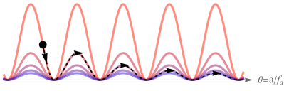
Figure 1: Schematic plot of the pNGB slide.

Unless the initial misalignment angle is small, our pNGB does not start oscillation even at $T\mathrel{\hbox to0.0pt{\lower 4.0pt\hbox{\hskip 1.0pt$\sim$}\hss}\raise 1.0pt\hbox{$<$}}T_{0}$. Instead, it slides along the potential (see Fig. 1). This is because the potential height of $\theta$ given by $m_{a}^{2}\propto T^{3}$ decreases faster than the redshift of the kinetic energy, $\dot{\theta}^{2}\propto T^{2}$. During this period, $\dot{\theta}/T$ is approximately constant since the right-hand side of Eq. (6) can be neglected due to the large kinetic energy, and the left-hand side is $\ddot{\theta}+H\dot{\theta}=T\frac{d}{dt}(\dot{\theta}/T)$.

If the initial misalignment angle is not sufficiently large, the pNGB may not slide as soon as $T$ approaches $T_{0}$ since the initial velocity $\dot{\theta}$ is too small to climb up the potential in the first motion. Then, it first oscillates a few times with $A^{2}m_{a}\propto T$ where $A$ denotes the amplitude of the pNGB oscillation, i.e. $\theta\simeq A(t)\cos[\int m_{a}\,dt]$. During this period, the kinetic energy of the oscillation $\dot{\theta}^{2}\simeq m_{a}^{2}A^{2}$ scales as $T^{5/2}$. As the potential barrier decreases faster, the kinetic energy becomes greater than the potential barrier at some point, and the pNGB starts sliding away. We estimate this sliding temperature as

$$T_{\rm slide}\simeq\mathcal{C}\frac{1}{4}T_{0}(1-\cos(5\theta_{i}))^{2},$$ (8)

with a numerical factor ${\cal C}\sim O(10)$ which depends on $T_{\rm RH}$ logarithmically with some power. In either case, $\dot{\theta}/T$ during the slide is constant and maximal in the history of the pNGB dynamics. Its value is given by

$$\bigg{(}\frac{\dot{\theta}}{T}\bigg{)}_{\rm\!\!slide}\!\!\!\!\!\!\!\simeq\frac{2m_{a}(T_{\rm slide})}{5T_{\rm slide}}$$ (9)

$$\simeq 7\times 10^{-8}\,{\cal C}^{1/2}(5\theta_{i})^{2}\bigg{(}\!\frac{100}{g_{*}}\!\bigg{)}^{\!\!\!1/2}\!\!\bigg{(}\!\frac{c_{\lambda}}{10^{8}}\!\bigg{)}^{\!\!\!3/2}\!\!\bigg{(}\!\frac{m_{a}^{(0)}}{\mathrm{eV}}\!\bigg{)}^{\!\!2}\!\bigg{(}\!\frac{10^{6}\,\mathrm{GeV}}{f_{a}^{(0)}}\!\bigg{)}^{\!\!3}.$$

We do not consider a case of $5\theta_{i}\mathrel{\hbox to0.0pt{\lower 4.0pt\hbox{\hskip 1.0pt$\sim$}\hss}\raise 1.0pt\hbox{$<$}}0.1$ for which the sliding temperature is too low.

Oscillation energy density As the temperature drops further $T<T_{c}$, $f_{a}$ and $m_{a}$ get saturated to the zero-temperature values. Then, $\dot{f}_{a}/f_{a}$ in Eq. (6) vanishes, so $\dot{\theta}$ scales as $\dot{\theta}\propto T^{3}$ when $\dot{\theta}>m_{a}^{(0)}$. The final oscillation starts when $\dot{\theta}(T_{\rm osc})\simeq\frac{2}{5}m_{a}^{(0)}$ from which we obtain

$$T_{\rm osc} \simeq\frac{4\,\mathrm{GeV}}{{\cal C}^{1/6}(5\theta_{i})^{2/3}}\bigg{(}\!\frac{g_{*}}{100}\!\bigg{)}^{\!\!\!1/6}\!\!\bigg{(}\!\frac{10^{8}}{c_{\lambda}}\!\bigg{)}^{\!\!\!5/6}\!\!\bigg{(}\!\frac{\mathrm{eV}}{m_{a}^{(0)}}\!\bigg{)}^{\!\!\!1/3}\!\!\bigg{(}\!\frac{f_{a}^{(0)}}{10^{6}\,\mathrm{GeV}}\!\bigg{)}^{\!\!5/3}\!\!\!.$$ (10)

This oscillation temperature is smaller than the typical oscillation temperature for constant $m_{a}$ and $f_{a}$ in the standard misalignment mechanism.

The ratio of the oscillation energy density and the entropy density is frozen as

$$\frac{\rho_{\rm osc}}{s}\simeq 2\times\frac{\frac{2}{25}\big{(}{m_{a}^{(0)}}{f_{a}^{(0)}}\big{)}^{2}}{s(T_{\rm osc})}$$ (11)

$$\simeq 0.07\,\mathrm{eV}\,{\cal C}^{1/2}{(5\theta_{i})^{2}}\bigg{(}\!\frac{100}{g_{*}}\!\bigg{)}^{\!\!\!3/2}\!\!\bigg{(}\!\frac{c_{\lambda}}{10^{8}}\!\bigg{)}^{\!\!\!5/2}\!\!\bigg{(}\!\frac{m_{a}^{(0)}}{\mathrm{eV}}\!\bigg{)}^{\!\!\!3}\!\bigg{(}\!\frac{10^{6}\,\mathrm{GeV}}{f_{a}^{(0)}}\!\bigg{)}^{\!\!3}\!\!,$$

where the factor $\simeq 2$ comes from our numerical checks (see Supplemental Material for details). Requiring $\rho_{\rm osc}/s=0.44\,\mathrm{eV}$  for the observed dark matter abundance Planck:2018vyg , one obtains the relation between $m_{a}^{(0)}$ and $f_{a}^{(0)}$ for a given $c_{\lambda}$.

Our scenario has similarities with those using the kinetic misalignment mechanism Co:2019wyp ; Co:2019jts ; Co:2020jtv ; Harigaya:2021txz ; Chakraborty:2021fkp ; Kawamura:2021xpu ; Co:2021qgl ; Co:2022aav ; Barnes:2022ren ; Co:2022kul ; Badziak:2023fsc ; Co:2020xlh ; Berbig:2023uzs ; Chun:2023eqc ; Chao:2023ojl ; Barnes:2024jap ; Datta:2024xhg . In both cases, the baryon-number-inducing pNGB rotation is generated at a high temperature and later the pNGB gets trapped, oscillates, and becomes dark matter. The difference lies in the dynamics of the radial mode $\phi$: in the kinetic misalignment mechanism, the radial mode is initially misaligned at a field value much greater than its potential minimum, and $\dot{\theta}$ is generated during the non-thermal evolution of $\phi$ rolling down toward the potential minimum, and afterward, $\dot{\theta}$ scales as $T^{3}$. In our scenario, $\dot{\theta}$ is generated while $\phi$ stays around its potential minimum adiabatically, and $\dot{\theta}$ scales as $T$ at $T>T_{c}$.

An explicit model To discuss how the successful baryogenesis arises, let us consider the type-I seesaw model extended with the Majoron as an example. The model Lagrangian includes

$$-\Delta{\cal L}=(y\Phi\nu^{c}\nu^{c}+Y_{D}Hl\nu^{c}+h.c.)+V(\Phi)$$ (12)

where $\nu^{c}$ and $l$ denote the anti-right-handed neutrino and the SM lepton doublet, respectively. The vev of $\Phi$ generates Majorana masses of $\nu^{c}$, $M_{N}=yf_{a}^{(0)}/\sqrt{2}$ and drives the seesaw mechanism to explain small neutrino masses.

In this setup, we apply the previous discussion to the $\Phi$ sector. That is, $\Phi$ receives a negative $T^{2}$ quadratic term, and its axial mode, the Majoron, plays the role of the pNGB in our cogenesis scenario.

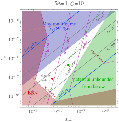
Figure 2: Constraints (shaded region) and relevant physical quantities (solid lines) are depicted in the plane of $\lambda_{\rm mix}=\lambda_{h\phi}+\lambda_{hs}/4$ and $\lambda_{\phi}$ for the Majoron model. The green-shaded region is excluded since the potential has an unstable direction. The blue-shaded region is excluded by the lower bound of the Majoron lifetime (CMB and BAO) Audren:2014bca ; Enqvist:2019tsa ; Nygaard:2020sow ; Alvi:2022aam ; Simon:2022ftd , and the BBN constraint on $\phi$ is depicted by the red-shaded region Fradette:2017sdd . Solid lines with different colors represent benchmark values of relevant physical quantities: $m_{\phi}$ in red, $c_{\lambda}$ in gray, $T_{c}$ in blue, and the naive $h$-$\phi$ mixing angle $\sin\tilde{\theta}_{h\phi}$ in purple. The regions indicated by the arrows are excluded in the minimal Higgs portal model, but they are still viable if singlet scalars are added.

The right-handed neutrino mass is given by $M_{N}(T)\simeq y\sqrt{c_{\lambda}}T/\sqrt{2}$ at high temperature. Since Yukawa coupling generates quantum and thermal corrections to the potential of $\phi$, we need to consider $y\sqrt{c_{\lambda}}\mathrel{\hbox to0.0pt{\lower 4.0pt\hbox{\hskip 1.0pt$\sim$}\hss}\raise 1.0pt\hbox{$<$}}4\pi$ and $y^{2}<4\lambda_{\rm mix}$ to avoid spoiling the previous discussion. We take $y\sim 1/\sqrt{c_{\lambda}}$ such that the right-handed neutrinos are in the thermal bath satisfying $M_{N}(T)/T\sim 1$ at $T>T_{c}\simeq f_{a}^{(0)}/\sqrt{c_{\lambda}}$. The zero temperature value of $M_{N}$ is set to be $yf_{a}^{(0)}/\sqrt{2}\sim T_{c}$. Consequently, its decay and inverse decay processes are active, and generate lepton asymmetry based on the nonzero $\dot{\theta}$, which is transported to the baryon asymmetry via the weak sphaleron Chun:2023eqc .

The baryon asymmetry is effectively frozen when either the electroweak sphaleron is decoupled at $T_{\rm EW}\simeq 130\,\mathrm{GeV}$ DOnofrio:2014rug ; Kuzmin:1985mm , or $M_{N}(T)/T$ becomes greater than $z_{\rm fo}\simeq 7$. The latter case happens around $T=M_{N}^{(0)}/z_{\rm fo}$ after $M_{N}(T)$ gets saturated at $M_{N}^{(0)}\simeq yf_{a}^{(0)}/\sqrt{2}$. So

$$Y_{B}=\!\frac{45c_{B}}{2\pi^{2}g_{*}}\bigg{(}\frac{\dot{\theta}}{T}\bigg{)}_{\rm\!\!slide}\!\!\!\!\!\!\!\times\begin{cases}1&\text{for $T_{\rm EW}>T_{c}$}\\ \big{(}\frac{T_{\rm EW}}{T_{c}}\big{)}^{2}&\text{for $M_{N}^{(0)}/z_{\rm fo}<T_{\rm EW}<T_{c}$}\\ \big{(}\frac{M_{N}^{(0)}}{z_{\rm fo}T_{c}}\big{)}^{2}&\text{for $T_{\rm EW}<M_{N}^{(0)}/z_{\rm fo}$}\end{cases}$$ (13)

where we find $c_{B}\simeq\frac{7}{33}$, and the suppression factors come from $T^{3}$ scaling of $\dot{\theta}$ during $T_{\rm osc}<T<T_{c}$. Using Eqs. (9) and (11), we obtain

$$m_{a}^{(0)}=\frac{5\,\mathrm{eV}}{{\cal C}^{1/9}(5\theta_{i})^{4/9}}\bigg{(}\!\frac{g_{*}}{100}\!\bigg{)}^{\!\!\!1/3}\!\!\bigg{(}\!\frac{10^{8}}{c_{\lambda}}\!\bigg{)}^{\!\!\!5/9},$$ (14)

$$f_{a}^{(0)}={3\times 10^{6}\,\mathrm{GeV}}\,\mathcal{C}^{1/18}{(5\theta_{i})^{2/9}}\bigg{(}\!\frac{100}{g_{*}}\!\bigg{)}^{\!\!\!1/6}\!\!\bigg{(}\!\frac{c_{\lambda}}{10^{8}}\!\bigg{)}^{\!\!\!5/18}\!\!,$$ (15)

taking the equation for $M_{N}^{(0)}/z_{\rm fo}<T_{\rm EW}<T_{c}$ which accidentally coincide with our case for $10^{7}\mathrel{\hbox to0.0pt{\lower 4.0pt\hbox{\hskip 1.0pt$\sim$}\hss}\raise 1.0pt\hbox{$<$}}c_{\lambda}\mathrel{\hbox to0.0pt{\lower 4.0pt\hbox{\hskip 1.0pt$\sim$}\hss}\raise 1.0pt\hbox{$<$}}10^{9}$.

The required $m_{a}^{(0)}$, $f_{a}^{(0)}$ and $T_{0}$ in Eq. (7) have tension with the isocurvature perturbation constraint from CMB observation Planck:2018jri . However, this can be easily avoided by introducing a small negative Hubble-induced mass Stewart:1994ts ; Dine:1995kz ; Dine:1995uk or coupling to the inflaton, making $f_{a}$ large during inflation without changing our scenario after reheating. As it is an independent sector, we leave detailed studies for future work. A related study was made in Ref. Chun:2014xva for the case of the QCD axion.

Once $\lambda_{\rm mix}$ and $\lambda_{\phi}$ are given, $c_{\lambda}\simeq\lambda_{\rm mix}/3\lambda_{\phi}$ is determined, so $m_{a}^{(0)}$ and $f_{a}^{(0)}$ are also fixed by Eqs. (14) and (15). Therefore, in Fig. 2, we present physically relevant quantities and their constraints in $\lambda_{\rm mix}$-$\lambda_{\phi}$ parameter space with taking $5\theta_{i}=O(1)$ and $M_{N}^{(0)}\simeq T_{c}$. First of all, the region shaded by green is excluded independently of the pNGB interactions since the potential is unstable due to the negative mixed quartic. The region below the green dashed line requires additional scalar fields with $O(1)$ self-quartic coupling to stabilize the potential. The blue-shaded region is excluded by the lifetime bound of the Majoron dark matter. It comes from analyses of the cosmic microwave background (CMB) and the baryon acoustic oscillation (BAO) Audren:2014bca ; Enqvist:2019tsa ; Nygaard:2020sow ; Alvi:2022aam ; Simon:2022ftd , whereas we take the current upper bound of neutrino masses $\sum m_{\nu}^{2}\simeq(0.05\,\mathrm{eV})^{2}$. This lifetime constraint can become stronger in $\lambda_{\phi}$-$\lambda_{\rm mix}$ plane by future neutrino mass measurements.

BBN also puts a strong constraint on $\phi$ as depicted by the red-shaded region Fradette:2017sdd . In this region, $\phi$ decays after BBN either because $m_{\phi}$ is smaller than the electron threshold $2m_{e}\simeq\mathrm{MeV}$, or $\sin\theta_{h\phi}$ is too small. Note that $\sin\theta_{h\phi}$ is not fully determined in this plane because $\lambda_{h\phi}=\lambda_{\rm mix}-N_{s}\lambda_{\phi s_{i}}/4$ depends on $\lambda_{\phi s_{i}}$ for a given $\lambda_{\rm mix}$. Assuming $\lambda_{h\phi}\sim N_{s}\lambda_{\phi s_{i}}/4\sim\lambda_{\rm mix}$, we naively estimate the mixing angle as $\tilde{\theta}_{h\phi}\sim 2\lambda_{\rm mix}f_{a}^{(0)}v_{h}/m_{h}^{2}$, and purple lines depict some of its benchmark values, $10^{-4}$, $10^{-5}$, and $10^{-6}$. For the minimal Higgs portal model, we expect $\tilde{\theta}_{h\phi}\simeq\theta_{h\phi}$, and therefore, the region left to $\sin\tilde{\theta}_{h\phi}=10^{-5}$ is excluded, but it can be rescued by additional scalars with $10\,\%$-level tuning between $\lambda_{h\phi}$ and $\lambda_{\phi s_{i}}$. For $\sin\tilde{\theta}_{h\phi}\mathrel{\hbox to0.0pt{\lower 4.0pt\hbox{\hskip 1.0pt$\sim$}\hss}\raise 1.0pt\hbox{$>$}}10^{-4}$, we have chances to prove our model via kaon experiments.

Other solid lines also represent values of relevant physical quantities. Red lines correspond to $m_{\phi}$, showing that $m_{\phi}\mathrel{\hbox to0.0pt{\lower 4.0pt\hbox{\hskip 1.0pt$\sim$}\hss}\raise 1.0pt\hbox{$<$}}20\,\mathrm{MeV}$ in our parameter space, gray lines represent several values of $c_{\lambda}$ and blue lines depict $T_{c}$ which is roughly the mass scale of the heaviest right-handed neutrino.

Note that, at $T>T_{c}$, $m_{\phi}(T)\sim\sqrt{\lambda_{\phi}c_{\lambda}}T$ is greater than the Hubble rate for $T<\sqrt{\lambda_{\phi}c_{\lambda}}M_{\rm Pl}$ in our temperature range. Therefore, the time scale of $\phi$ dynamics is short enough, and its oscillation effects on the $\theta$ dynamics should be averaged out, which justifies $\phi=f_{a}$ treatment in Eq. (6). Moreover, the $\phi$ oscillation gets quickly damped out by the thermal friction of $\Gamma\sim y^{2}T$ with $y\sim 10^{-4}$, which makes $\phi$ adiabatically follow $f_{a}$.

Summary In this Letter, we have found that an initial misalignment of a pNGB can successfully generate the observed baryon asymmetry as well as dark matter abundance if the pNGB potential decreases as the temperature drops. This required property can be realized by the non-restoration of the corresponding global symmetry with a dimension-five explicit breaking operator. In this setup, as the potential rapidly decreases as temperature drops, the pNGB initially slides along the potential, during which sufficiently large baryon asymmetry can be generated. After the potential becomes saturated below $T_{c}$, the pNGB gets trapped in its potential, starts oscillation, and becomes dark matter.

We have explicitly shown that this idea can be realized by the Majoron in the type-I seesaw model whose working parameter space is summarized in Fig. 2. After all, our Majoron scenario predicts (i) a scalar field $\phi$ with $\mathrm{MeV}<m_{\phi}\mathrel{\hbox to0.0pt{\lower 4.0pt\hbox{\hskip 1.0pt$\sim$}\hss}\raise 1.0pt\hbox{$<$}}20\,\mathrm{MeV}$ and $10^{-5}\mathrel{\hbox to0.0pt{\lower 4.0pt\hbox{\hskip 1.0pt$\sim$}\hss}\raise 1.0pt\hbox{$<$}}\sin\theta_{h\phi}\mathrel{\hbox to0.0pt{\lower 4.0pt\hbox{\hskip 1.0pt$\sim$}\hss}\raise 1.0pt\hbox{$<$}}10^{-4}$, (ii) a right-handed neutrino with $10\,\mathrm{GeV}\mathrel{\hbox to0.0pt{\lower 4.0pt\hbox{\hskip 1.0pt$\sim$}\hss}\raise 1.0pt\hbox{$<$}}M_{N}^{(0)}\mathrel{\hbox to0.0pt{\lower 4.0pt\hbox{\hskip 1.0pt$\sim$}\hss}\raise 1.0pt\hbox{$<$}}400\,\mathrm{GeV}$, and (iii) Majoron dark matter with $m_{a}^{(0)}\sim\mathrm{eV}$ and $f_{a}^{(0)}\sim 10^{6}\,\mathrm{GeV}$ whose lifetime is slightly greater than $250\,{\rm Gyr}$.

These predictions can be tested in multiple directions. The upper bound of $\sin\theta_{h\phi}$ in our mass range is expected to be probed up to $\sin\theta_{\phi h}\mathrel{\hbox to0.0pt{\lower 4.0pt\hbox{\hskip 1.0pt$\sim$}\hss}\raise 1.0pt\hbox{$<$}}4\times 10^{-5}$ by $K_{L}$ experiments such as KOTO step-2 Goudzovski:2022vbt ; Nomura:2020oor ; Aoki:2021cqa and KLEVER Goudzovski:2022vbt ; Beacham:2019nyx , and weak-scale right-handed neutrinos can be tested in future colliders Chun:2019nwi ; Abdullahi:2022jlv . Furthermore, in the non-minimal model, the singlet scalar fields must interact with the SM sector to be in the thermal bath and decay into the SM particles to avoid strong cosmological constraints with a lifetime shorter than $0.1\,\sec$. Although there is an arbitrariness in their interactions, their masses are expected to be around the electroweak scale to avoid tuning of $\Phi$ and Higgs potential. These particles can be tested at the LHC in various channels CMS:2024zqs ; ATL-PHYS-PUB-2022-007 ; ATL-PHYS-PUB-2023-008 ; ATL-PHYS-PUB-2023-018 and future colliders Bernardi:2022hny ; Narain:2022qud ; ILCInternationalDevelopmentTeam:2022izu ; ILC:2013jhg ; Bambade:2019fyw ; Linssen:2012hp ; CLICdp:2018cto ; FCC:2018evy ; CEPCStudyGroup:2018ghi ; CEPCPhysicsStudyGroup:2022uwl ; FCC:2018vvp .

On the other hand, constraining $\mathrm{eV}$-scale Majoron dark matter seems difficult. Although there are severe constraints on thermally produced Majorons Sabti:2019mhn ; Blinov:2019gcj ; Sandner:2023ptm ; Chang:2024mvg , their abundance is highly suppressed in our parameter space, $c_{\lambda}>10^{7}$, and these constraints cannot be applied.

Acknowledgement We would like to thank Takeo Moroi and Kyohei Mukaida for useful comments. This work was supported by IBS under the project code, IBS-R018-D1.

Supplemental Material

S1 1. Realizing a large $c_{\lambda}$

S1.1 Model

For simplicity, let us consider a scalar model

$$V(\Phi,S) =\lambda_{\phi}|\Phi|^{4}-2\lambda_{\phi s}|\Phi|^{2}|S|^{2}+\lambda_{s}|S|^{4}$$

$$-m_{0}^{2}|\Phi|^{2}+m_{s}^{2}|S|^{2},$$ (S1)

where $S$ is an additional complex scalar with $\lambda_{\phi},\,\lambda_{\phi s},\,\lambda_{s},\,m_{0}^{2},\,m_{s}^{2}>0$. One can trivially replace $S$ by the SM Higgs doublet $H$ with proper treatments of Higgs vacuum expectation value (vev) and mass conditions and degrees of freedom.

Let us denote the radial modes of $\Phi$ and $S$ by $\phi$ and $s$, respectively. Their potential is given by

$$V=\frac{1}{4}\lambda_{\phi}\phi^{4}-\frac{1}{2}(m_{0}^{2}+\lambda_{\phi s}s^{2})\phi^{2}+\frac{1}{4}\lambda_{s}s^{4}+\frac{1}{2}m_{s}^{2}s^{2}.$$ (S2)

At each slice of constant $s$, $V$ is minimized at $\phi^{2}=(m_{0}^{2}+\lambda_{\phi s}s^{2})/\lambda_{\phi}$. Putting this back to the potential gives the potential along this trajectory,

$$V\to-\frac{(m_{0}^{2}+\lambda_{\phi s}s^{2})^{2}}{4\lambda_{\phi}}+\frac{1}{4}\lambda_{s}s^{4}+\frac{1}{2}m_{s}^{2}s^{2}.$$ (S3)

For the stability of the potential at large $s$, we need the effective quartic term to be positive, which can be written as

$$\lambda_{\phi}\lambda_{s}-\lambda_{\phi s}^{2}>0.$$ (S4)

In addition, to make $\langle s\rangle=0$ (although it is not necessary), we require the quadratic term to be positive, so

$$m_{s}^{2}>\frac{\lambda_{\phi s}}{\lambda_{\phi}}m_{0}^{2}\sim\lambda_{\phi s}\,{f_{a}^{(0)}}^{2}.$$ (S5)

For the Higgs case, one needs to solve the conditions of $v_{h}=246\,\mathrm{GeV}$ and $m_{h}=125\,\mathrm{GeV}$, which fixes the quadratic and quartic couplings as functions of $f_{a}^{(0)}$ and $\lambda_{h\phi}$. However, these conditions may not be sufficient, since the potential can be spoiled by radiative corrections. In the next subsection, we will check self-consistency numerically by including the Colemann-Weinberg potential which is given by

$$V_{\rm CW} =\frac{1}{64\pi^{2}}\Bigg{[}(3\lambda_{\phi}\phi^{2}-\lambda_{\phi s}s^{2}-m_{0}^{2})^{2}\Big{(}\log\frac{3\lambda_{\phi}\phi^{2}-\lambda_{\phi s}s^{2}-m_{0}^{2}}{\mu^{2}}-\frac{3}{2}\Big{)}$$

$$~{}\qquad\qquad+(\lambda_{\phi}\phi^{2}-\lambda_{\phi s}s^{2}-m_{0}^{2})^{2}\Big{(}\log\frac{\lambda_{\phi}\phi^{2}-\lambda_{\phi s}s^{2}-m_{0}^{2}}{\mu^{2}}-\frac{3}{2}\Big{)}$$

$$~{}\qquad\qquad+(3\lambda_{s}s^{2}-\lambda_{\phi s}\phi^{2}+m_{s}^{2})^{2}\Big{(}\log\frac{3\lambda_{s}s^{2}-\lambda_{\phi s}\phi^{2}+m_{s}^{2}}{\mu^{2}}-\frac{3}{2}\Big{)}$$

$$~{}\qquad\qquad+(\lambda_{s}s^{2}-\lambda_{\phi s}\phi^{2}+m_{s}^{2})^{2}\Big{(}\log\frac{\lambda_{s}s^{2}-\lambda_{\phi s}\phi^{2}+m_{s}^{2}}{\mu^{2}}-\frac{3}{2}\Big{)}\Bigg{]}.$$ (S6)

In order to keep our analysis determined by the tree-level potential, we need $V_{\rm CW}$ to be small compared to the tree-level. For this, we need $\lambda\gg\lambda^{\prime}\lambda^{\prime\prime}/16\pi^{2}$ (with $\lambda,\lambda^{\prime},\lambda^{\prime\prime}=\lambda_{\phi},\lambda_{\phi s}$ or $\lambda_{s}$). Once it is satisfied, one-loop contributions become sufficiently small compared to the tree-level potential except for the $\lambda_{\phi s}m_{s}^{2}\phi^{2}$ term from the third and fourth lines of (S6). Therefore, the vev of $\phi$ should be estimated with

$$m_{\phi}^{2} =m_{0}^{2}+\frac{\lambda_{\phi s}}{16\pi^{2}}m_{s}^{2}\log\frac{m_{s}^{2}}{\mu^{2}}$$ (S7)

$$\langle\phi\rangle \equiv f_{a}^{(0)}\simeq\frac{m_{\phi}}{\sqrt{\lambda_{\phi}}},$$ (S8)

which brings $m_{s}$ to be as small as possible unless we finely tune the parameters $m_{0}^{2}$ and $m_{s}^{2}$ (this tuning may be acceptable since we anyway ignore all the UV corrections to scalar masses). When we take the smallest value of (S5), the correction to $m_{\phi}^{2}$ is roughly $\delta m_{\phi}^{2}/m_{\phi}^{2}\sim O(\lambda_{\phi s}^{2}/(16\pi^{2}\lambda_{\phi}))\mathrel{\hbox to0.0pt{\lower 4.0pt\hbox{\hskip 1.0pt$\sim$}\hss}\raise 1.0pt\hbox{$<$}}O(1)$.

With $\langle s\rangle=0$, we have the temperature-dependent potential

$$V_{T}(\phi) =\frac{\lambda_{\phi}}{4}\phi^{4}-\frac{m_{0}^{2}}{2}\phi^{2}+\left.V_{\rm CW}\right|_{s=0}$$ (S9)

$$+\frac{T^{4}}{2\pi^{2}}J_{B}\left(\frac{3\lambda_{\phi}\phi^{2}-m_{0}^{2}}{T^{2}}\right)+\frac{T^{4}}{2\pi^{2}}J_{B}\left(\frac{\lambda_{\phi}\phi^{2}-m_{0}^{2}}{T^{2}}\right)+2\cdot\frac{T^{4}}{2\pi^{2}}J_{B}\left(\frac{m_{s}^{2}-\lambda_{\phi s}\phi^{2}}{T^{2}}\right),$$ (S10)

where $J_{B}$ is the thermal correction from a bosonic degree, defined as

$$J_{B}(m^{2}/T^{2}) =\int_{0}^{\infty}dx\,x^{2}\log\left(1-e^{-\sqrt{x^{2}+m^{2}/T^{2}}}\right),$$ (S11)

and its high-$T$ expansion can be written as

$$J_{B}(m^{2}/T^{2}) \simeq-\frac{\pi^{4}}{45}+\frac{\pi^{2}}{12}\frac{m^{2}}{T^{2}}+\cdots.$$ (S12)

Therefore, at a high temperature with $T\gg m_{s}$ and $T\gg\sqrt{\lambda_{\phi s}}\phi$, we can expand Eq. (S11) as

$$V_{T}(\phi) \simeq\frac{\lambda_{\phi}}{4}\phi^{4}-\frac{m^{2}}{2}\phi^{2}+V_{CW}+\bigg{(}-4\cdot\frac{\pi^{2}}{90}T^{4}+\frac{T^{2}}{24}\bigg{(}(3\lambda_{\phi}\phi^{2}-m^{2})+(\lambda_{\phi}\phi^{2}-m^{2})+2(m_{s}^{2}-\lambda_{\phi s}\phi^{2})\bigg{)}+\cdots\bigg{)}$$ (S13)

$$\simeq\frac{\lambda_{\phi}}{4}\phi^{4}-\frac{1}{2}\bigg{(}m_{\phi}^{2}+\frac{\lambda_{\phi s}-2\lambda_{\phi}}{6}T^{2}\bigg{)}\phi^{2}+\cdots.$$ (S14)

In the final expression, we have ignored constant terms and the Colemenn-Weinberg potential except for the quadratic correction. Therefore, we obtain

$$c_{\lambda}=\frac{N_{s}\lambda_{\phi s}-4\lambda_{\phi}}{12\lambda_{\phi}},$$ (S15)

where $N_{s}$ is the degree of freedom of $S$. When $S$ is a complex scalar field as we set here, $N_{s}=2$ while $N_{s}=4$ should be taken if one replaces $S$ by the SM Higgs doublet $H$. Note that, to have $c_{\lambda}>0$, we need $\lambda_{\phi s}>2\lambda_{\phi}$.

On the other hand, $S$ has to be in the thermal bath to provide thermal corrections. If $S$ were the Higgs boson, we do not need to introduce additional interactions, but for $S$, this can be realized by a mixed quartic coupling between $S$ and the SM Higgs doublet $H$,

$$\lambda_{hs}|H|^{2}|S|^{2},$$ (S16)

from which the production rate of $S$ is given by $\Gamma\sim\lambda_{hs}^{2}T$. Having it to be greater than the Hubble rate at $T\simeq T_{\rm EW}$ ($T_{0}$) provides a lower bound of $\lambda_{hs}\mathrel{\hbox to0.0pt{\lower 4.0pt\hbox{\hskip 1.0pt$\sim$}\hss}\raise 1.0pt\hbox{$>$}}10^{-8}$ ($10^{-3}$). Of course, one can introduce other interactions instead of (S16).

S1.2 Numerical study

To realize a large $c_{\lambda}$, we need $\lambda_{\phi s}\gg\lambda_{\phi}$, but we have to satisfy the stability condition (S4), which can be rewritten as

$$c_{\lambda}\simeq\frac{\lambda_{\phi s}}{6\lambda_{\phi}}<\frac{\lambda_{s}}{6\lambda_{\phi s}},$$ (S17)

so we have to take a large $\lambda_{s}$ and a small $\lambda_{\phi s}$. At the same time, $\lambda_{\phi}$ must be $O(\lambda_{\phi s}^{2})$ to maximize $c_{\lambda}$.

Here, we chose benchmark parameters to provide $c_{\lambda}\simeq 10^{8}$;

$$\lambda_{\phi s}=\frac{1}{6}\times 10^{-9},\quad\lambda_{\phi}=10\lambda_{\phi s}^{2},\quad\lambda_{s}=1,\quad m_{s}=\sqrt{2\lambda_{\phi s}}f_{a}^{(0)},\quad m_{0}=\sqrt{\lambda_{\phi}}f_{a}^{(0)}$$ (S18)

Note that changing these parameters to make $c_{\lambda}>10^{8}$ is not difficult at all. We take $\mu=f_{a}^{(0)}$ in the following analysis.

First, we check that $\langle s\rangle=0$, and the zero-temperature potential is not spoiled by quantum corrections. We include the full expression of the Colemann-Weinberg correction given in Eq. (S6) and depict it in Fig. S3. $V^{1/4}$ is depicted in $\phi$-$s$ space in the left panel, and the potential in the $\phi$ direction is depicted for fixed $s/f_{a}^{(0)}=10^{-3},\,10^{-2},\,10^{-1},\,1,$ and $10$. As shown in the figures, the potential is minimized at $\langle\phi\rangle\simeq f_{a}^{(0)}$, and there is no minimum at nonzero $s$.

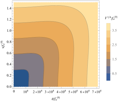
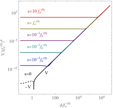
Figure S3: [Left] One-quarter power of the zero temperature potential is depicted in $\phi$-$s$ space. As it is shown, there is no unstable direction. [Right] The potential in the $\phi$ direction is depicted for fixed $s/f_{a}^{(0)}=10^{-3},\,10^{-2},\,10^{-1},\,1,$ and $10$.

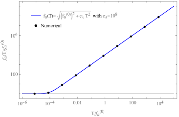
Figure S4: [Left] $V(\phi)$ with $s=0$ is depicted for different temperatures, $T=0,\,2T_{c},$ and $3T_{c}$. [Right] $f_{a}(T)=\langle\phi\rangle_{T}$ is depicted as a function of temperature. Black dots indicate the values we obtained by minimizing the full one-loop temperature-dependent effective potential while the blue line corresponds to the expected line from the approximated effective potential.

With taking $s=0$, the temperature-dependent potential $V_{T}(\phi)$ is depicted in the left panel of Fig. S4. In the figure, we fix $V(0)=0$ by a constant shift to make a comparison among different temperatures. We scan temperatures and find $\langle\phi\rangle_{T}$ at each temperature. Our numerical finding is shown by black dots in the right panel of Fig. S4, which make good agreement with our analytic expression $f_{a}(T)\simeq\sqrt{(f_{a}^{(0)})^{2}+c_{\lambda}T^{2}}$ with taking $c_{\lambda}=10^{8}$ as depicted by the solid blue line.

S2 2. Numerical study of pNGB dynamics

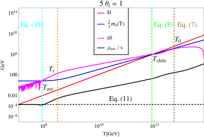
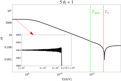
Figure S5: Left panel: Evolution of $H$, $\frac{2}{5}m_{a}(T)$, $|\dot{\theta}|$ and $\rho_{\rm osc}/s$ with temperature considering $f_{a}^{(0)}=10^{10}~{}\text{GeV}$, $m_{a}^{(0)}=19~{}\text{GeV}$, $c_{\lambda}=10^{3}$ and $5\theta_{i}=1$. Right panel: Evolution of $|\theta|$ for the same parameters.

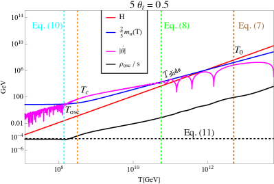
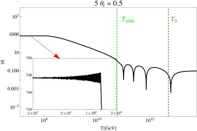
Figure S6: Same as in Fig. S5, but for $5\theta_{i}=0.2$.

Here, we demonstrate the dynamics of $\theta$ in the different regimes by numerically solving its equation of motion (cf. Eq. (6)) and check the consistency of our analytical estimates derived in the main text. We present our numerical results in Figs. S5-S7, choosing some benchmark parameters. In Fig. S5, we consider $5\theta_{i}=1$. In this case, after the Hubble friction term becomes small enough compared to the mass term, the pNGB goes to the minimum of the potential and subsequently crosses the barrier when the kinetic energy becomes equal to the potential barrier, i.e. $\frac{1}{2}\dot{\theta}^{2}(T)=\frac{2m_{a}^{2}(T)}{25}$. It then starts to slide across the rapidly decreasing potential barriers (cf. Fig. 1). The left panel shows the evolution of the Hubble rate $H$, the temperature-dependent mass $m_{a}(T)\times\frac{2}{5}$, the velocity $|\dot{\theta}|$ and the comoving energy density of the oscillation $\rho_{\rm osc}/s$. The scaling of $|\dot{\theta}|$ (magenta contour) changes from $T$ to $T^{3}$ after $T_{c}$, and finally the pNGB starts to oscillate when the velocity becomes comparable to the mass $m_{a}^{(0)}$(blue contour). On the other hand, the oscillation energy density (black contour) keeps on diluting until it becomes constant after $T_{\rm osc}$. The right panel shows the evolution of $\theta$, which is frozen initially at the value $\theta_{i}$. It increases after the temperature reaches $T_{\rm slide}$, since it continues to cross the potential barriers as discussed above. The oscillation of the pNGB after $T_{\rm osc}$, can be seen clearly in the magnified inset plot. The different dashed lines in the figures indicate our analytical estimates of $T_{0}$, $T_{\rm slide}$, $T_{\rm osc}$ and $\rho_{\rm osc}/s$, given by Eq. (7), (8), (10) and (11) respectively, and we consider $T_{c}=f_{a}^{0}/\sqrt{c_{\lambda}}$. Starting from a reheating temperature $T_{\rm RH}\simeq 10~{}T_{0}$, we find that $\mathcal{C}\simeq 3$ in the determination of $T_{\rm slide}$ (cf. Eq. (8)) provides a good estimate in order to match with our numerical results.

In Fig. S6, we show the behavior for a smaller value of the initial angle, considering $5\theta_{i}=0.5$. Consequently, our pNGB cannot cross the barrier after reaching the minimum from the initial displaced value. Rather, it oscillates until the kinetic energy equals the potential barrier, after which it starts to slide, following the same behavior as in Fig. S5, but with a relatively smaller oscillation energy density. Note that our predictions of the physical behavior of the pNGB, including its energy density given by Eq. (11), match adequately with our numerical solution. Thus, although solving the equation numerically for a large hierarchy between $T_{0}$ and $T_{\rm osc}$ becomes computationally too heavy for our purpose, the dynamics remain the same as shown in Fig. S5, S6, and hence we can conclude to arrive at similar results given by our analytical formulas.

Finally, to verify our results further, we show the behavior of $|\dot{\theta}|/T$ for a wide range of our parameters and compare it with our analytical formula (cf. Eq. (9)) at $T_{\rm slide}$. For instance, we vary the pNGB mass $m_{a}^{(0)}$ from eV to the GeV scale. The results are shown in Fig. S7, for $5\theta_{i}=1$ (left panel) and $5\theta_{i}=0.2$ (right panel). The solid lines indicate the evolution of the $|\dot{\theta}|/T$ obtained numerically for different choices of benchmark values covering a wide range. The dashed horizontal line represents the analytical estimate, given by Eq. (9). We again find that $C\simeq 3$, considering $T_{\rm RH}\simeq 10~{}T_{0}$. The vertical dashed lines represent our analytical estimates of the temperatures at the boundaries of the different regimes, which again, we find to agree reasonably well with our numerical results.

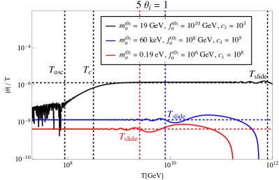
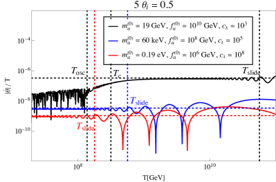
Figure S7: Evolution of $|\dot{\theta}|/T$ for different benchmark parameters considering $5\theta_{i}=1$ (left panel) and $5\theta_{i}=0.2$ (right panel). The solid lines indicate the results from our numerical solutions while the dashed lines represent our analytical estimates.

References

- (1) Planck collaboration, Planck 2018 results. VI. Cosmological parameters, Astron. Astrophys. 641 (2020) A6 [1807.06209].
- (2) A.D. Sakharov, Violation of CP Invariance, C asymmetry, and baryon asymmetry of the universe, Pisma Zh. Eksp. Teor. Fiz. 5 (1967) 32.
- (3) G. Elor et al., New Ideas in Baryogenesis: A Snowmass White Paper, in Snowmass 2021, 3, 2022 [2203.05010].
- (4) A.G. Cohen and D.B. Kaplan, Thermodynamic Generation of the Baryon Asymmetry, Phys. Lett. B 199 (1987) 251.
- (5) A.G. Cohen and D.B. Kaplan, SPONTANEOUS BARYOGENESIS, Nucl. Phys. B 308 (1988) 913.
- (6) V. Domcke, Y. Ema, K. Mukaida and M. Yamada, Spontaneous Baryogenesis from Axions with Generic Couplings, JHEP 08 (2020) 096 [2006.03148].
- (7) K.S. Jeong, T.H. Jung and C.S. Shin, Axionic Electroweak Baryogenesis, Phys. Lett. B 790 (2019) 326 [1806.02591].
- (8) K.S. Jeong, T.H. Jung and C.S. Shin, Adiabatic electroweak baryogenesis driven by an axionlike particle, Phys. Rev. D 101 (2020) 035009 [1811.03294].
- (9) K. Harigaya and I.R. Wang, ALP-assisted strong first-order electroweak phase transition and baryogenesis, JHEP 04 (2024) 108 [2309.00587].
- (10) I. Affleck and M. Dine, A New Mechanism for Baryogenesis, Nucl. Phys. B 249 (1985) 361.
- (11) R.T. Co and K. Harigaya, Axiogenesis, Phys. Rev. Lett. 124 (2020) 111602 [1910.02080].
- (12) R.T. Co, L.J. Hall and K. Harigaya, Axion Kinetic Misalignment Mechanism, Phys. Rev. Lett. 124 (2020) 251802 [1910.14152].
- (13) J. Preskill, M.B. Wise and F. Wilczek, Cosmology of the Invisible Axion, Phys. Lett. B 120 (1983) 127.
- (14) L.F. Abbott and P. Sikivie, A Cosmological Bound on the Invisible Axion, Phys. Lett. B 120 (1983) 133.
- (15) M. Dine and W. Fischler, The Not So Harmless Axion, Phys. Lett. B 120 (1983) 137.
- (16) E.J. Chun and T.H. Jung, Leptogenesis driven by majoron, 2311.09005.
- (17) S. Weinberg, Gauge and Global Symmetries at High Temperature, Phys. Rev. D 9 (1974) 3357.
- (18) R.N. Mohapatra and G. Senjanovic, Soft CP Violation at High Temperature, Phys. Rev. Lett. 42 (1979) 1651.
- (19) Y. Fujimoto and S. Sakakibara, ON SYMMETRY NONRESTORATION AT HIGH TEMPERATURE, Phys. Lett. B 151 (1985) 260.
- (20) P. Salomonson, B.S. Skagerstam and A. Stern, On the Primordial Monopole Problem in Grand Unified Theories, Phys. Lett. B 151 (1985) 243.
- (21) G. Bimonte and G. Lozano, On Symmetry nonrestoration at high temperature, Phys. Lett. B 366 (1996) 248 [hep-th/9507079].
- (22) G.R. Dvali, A. Melfo and G. Senjanovic, Is There a monopole problem?, Phys. Rev. Lett. 75 (1995) 4559 [hep-ph/9507230].
- (23) G.R. Dvali, A. Melfo and G. Senjanovic, Nonrestoration of spontaneously broken P and CP at high temperature, Phys. Rev. D 54 (1996) 7857 [hep-ph/9601376].
- (24) J. Orloff, The UV price for symmetry nonrestoration, Phys. Lett. B 403 (1997) 309 [hep-ph/9611398].
- (25) M.B. Gavela, O. Pene, N. Rius and S. Vargas-Castrillon, The Fading of symmetry nonrestoration at finite temperature, Phys. Rev. D 59 (1999) 025008 [hep-ph/9801244].
- (26) B. Bajc and G. Senjanovic, High temperature symmetry breaking via flat directions, Phys. Rev. D 61 (2000) 103506 [hep-ph/9811321].
- (27) J.R. Espinosa, M. Losada and A. Riotto, Symmetry nonrestoration at high temperature in little Higgs models, Phys. Rev. D 72 (2005) 043520 [hep-ph/0409070].
- (28) A. Ahriche, The Restoration of the Electroweak Symmetry at High Temperature for Little Higgs, 1003.5045.
- (29) C. Kilic and S. Swaminathan, Can A Pseudo-Nambu-Goldstone Higgs Lead To Symmetry Non-Restoration?, JHEP 01 (2016) 002 [1508.05121].
- (30) P. Meade and H. Ramani, Unrestored Electroweak Symmetry, Phys. Rev. Lett. 122 (2019) 041802 [1807.07578].
- (31) I. Baldes and G. Servant, High scale electroweak phase transition: baryogenesis \& symmetry non-restoration, JHEP 10 (2018) 053 [1807.08770].
- (32) A. Glioti, R. Rattazzi and L. Vecchi, Electroweak Baryogenesis above the Electroweak Scale, JHEP 04 (2019) 027 [1811.11740].
- (33) O. Matsedonskyi and G. Servant, High-Temperature Electroweak Symmetry Non-Restoration from New Fermions and Implications for Baryogenesis, JHEP 09 (2020) 012 [2002.05174].
- (34) O. Matsedonskyi, High-Temperature Electroweak Symmetry Breaking by SM Twins, JHEP 04 (2021) 036 [2008.13725].
- (35) P. Agrawal and M. Nee, Avoided deconfinement in Randall-Sundrum models, JHEP 10 (2021) 105 [2103.05646].
- (36) T. Biekötter, S. Heinemeyer, J.M. No, M.O. Olea and G. Weiglein, Fate of electroweak symmetry in the early Universe: Non-restoration and trapped vacua in the N2HDM, JCAP 06 (2021) 018 [2103.12707].
- (37) M. Carena, C. Krause, Z. Liu and Y. Wang, New approach to electroweak symmetry nonrestoration, Phys. Rev. D 104 (2021) 055016 [2104.00638].
- (38) O. Matsedonskyi, J. Unwin and Q. Wang, Electroweak symmetry non-restoration from dark matter, JHEP 12 (2021) 167 [2107.07560].
- (39) J.H. Chang, M.O. Olea-Romacho and E.H. Tanin, Electroweak asymmetric early Universe via a scalar condensate, Phys. Rev. D 106 (2022) 113003 [2210.05680].
- (40) J.H. Chang, K.S. Jeong, C.H. Lee and C.S. Shin, Dynamical Generation of the Baryon Asymmetry from a Scale Hierarchy, 2401.13734.
- (41) A. Fradette and M. Pospelov, BBN for the LHC: constraints on lifetimes of the Higgs portal scalars, Phys. Rev. D 96 (2017) 075033 [1706.01920].
- (42) E. Goudzovski et al., New physics searches at kaon and hyperon factories, Rept. Prog. Phys. 86 (2023) 016201 [2201.07805].
- (43) K. Choi and S.H. Im, Constraints on Relaxion Windows, JHEP 12 (2016) 093 [1610.00680].
- (44) T. Flacke, C. Frugiuele, E. Fuchs, R.S. Gupta and G. Perez, Phenomenology of relaxion-Higgs mixing, JHEP 06 (2017) 050 [1610.02025].
- (45) J. Beacham et al., Physics Beyond Colliders at CERN: Beyond the Standard Model Working Group Report, J. Phys. G 47 (2020) 010501 [1901.09966].
- (46) P. Agrawal et al., Feebly-interacting particles: FIPs 2020 workshop report, Eur. Phys. J. C 81 (2021) 1015 [2102.12143].
- (47) NA62 collaboration, Measurement of the very rare K+→ decay, JHEP 06 (2021) 093 [2103.15389].
- (48) NA62 collaboration, Search for decays to invisible particles, JHEP 02 (2021) 201 [2010.07644].
- (49) NA62 collaboration, Search for a feebly interacting particle in the decay , JHEP 03 (2021) 058 [2011.11329].
- (50) BNL-E949 collaboration, Study of the decay in the momentum region MeV/c, Phys. Rev. D 79 (2009) 092004 [0903.0030].
- (51) KOTO collaboration, Search for the and decays at the J-PARC KOTO experiment, Phys. Rev. Lett. 122 (2019) 021802 [1810.09655].
- (52) KOTO collaboration, Study of the Decay at the J-PARC KOTO Experiment, Phys. Rev. Lett. 126 (2021) 121801 [2012.07571].
- (53) T. Kitahara, T. Okui, G. Perez, Y. Soreq and K. Tobioka, New physics implications of recent search for at KOTO, Phys. Rev. Lett. 124 (2020) 071801 [1909.11111].
- (54) R.T. Co, N. Fernandez, A. Ghalsasi, L.J. Hall and K. Harigaya, Lepto-Axiogenesis, JHEP 03 (2021) 017 [2006.05687].
- (55) K. Harigaya and I.R. Wang, Axiogenesis from phase transition, JHEP 10 (2021) 022 [2107.09679].
- (56) S. Chakraborty, T.H. Jung and T. Okui, Composite neutrinos and the QCD axion: Baryogenesis, dark matter, small Dirac neutrino masses, and vanishing neutron electric dipole moment, Phys. Rev. D 105 (2022) 015024 [2108.04293].
- (57) J. Kawamura and S. Raby, Lepto-axiogenesis in minimal SUSY KSVZ model, JHEP 04 (2022) 116 [2109.08605].
- (58) R.T. Co, K. Harigaya, Z. Johnson and A. Pierce, R-parity violation axiogenesis, JHEP 11 (2021) 210 [2110.05487].
- (59) R.T. Co, T. Gherghetta and K. Harigaya, Axiogenesis with a heavy QCD axion, JHEP 10 (2022) 121 [2206.00678].
- (60) P. Barnes, R.T. Co, K. Harigaya and A. Pierce, Lepto-axiogenesis and the scale of supersymmetry, JHEP 05 (2023) 114 [2208.07878].
- (61) R.T. Co, V. Domcke and K. Harigaya, Baryogenesis from decaying magnetic helicity in axiogenesis, JHEP 07 (2023) 179 [2211.12517].
- (62) M. Badziak and K. Harigaya, Naturally astrophobic QCD axion, JHEP 06 (2023) 014 [2301.09647].
- (63) R.T. Co, L.J. Hall and K. Harigaya, Predictions for Axion Couplings from ALP Cogenesis, JHEP 01 (2021) 172 [2006.04809].
- (64) M. Berbig, Diraxiogenesis, JHEP 01 (2024) 061 [2307.14121].
- (65) W. Chao and Y.-Q. Peng, Majorana Majoron and the Baryon Asymmetry of the Universe, 2311.06469.
- (66) P. Barnes, R.T. Co, K. Harigaya and A. Pierce, Lepto-axiogenesis with light right-handed neutrinos, 2402.10263.
- (67) A. Datta, S.K. Manna and A. Sil, Spontaneous Leptogenesis with sub-GeV Axion Like Particles, 2405.07003.
- (68) B. Audren, J. Lesgourgues, G. Mangano, P.D. Serpico and T. Tram, Strongest model-independent bound on the lifetime of Dark Matter, JCAP 12 (2014) 028 [1407.2418].
- (69) K. Enqvist, S. Nadathur, T. Sekiguchi and T. Takahashi, Constraints on decaying dark matter from weak lensing and cluster counts, JCAP 04 (2020) 015 [1906.09112].
- (70) A. Nygaard, T. Tram and S. Hannestad, Updated constraints on decaying cold dark matter, JCAP 05 (2021) 017 [2011.01632].
- (71) S. Alvi, T. Brinckmann, M. Gerbino, M. Lattanzi and L. Pagano, Do you smell something decaying? Updated linear constraints on decaying dark matter scenarios, JCAP 11 (2022) 015 [2205.05636].
- (72) T. Simon, G. Franco Abellán, P. Du, V. Poulin and Y. Tsai, Constraining decaying dark matter with BOSS data and the effective field theory of large-scale structures, Phys. Rev. D 106 (2022) 023516 [2203.07440].
- (73) M. D’Onofrio, K. Rummukainen and A. Tranberg, Sphaleron Rate in the Minimal Standard Model, Phys. Rev. Lett. 113 (2014) 141602 [1404.3565].
- (74) V.A. Kuzmin, V.A. Rubakov and M.E. Shaposhnikov, On the Anomalous Electroweak Baryon Number Nonconservation in the Early Universe, Phys. Lett. B 155 (1985) 36.
- (75) Planck collaboration, Planck 2018 results. X. Constraints on inflation, Astron. Astrophys. 641 (2020) A10 [1807.06211].
- (76) E.D. Stewart, Inflation, supergravity and superstrings, Phys. Rev. D 51 (1995) 6847 [hep-ph/9405389].
- (77) M. Dine, L. Randall and S.D. Thomas, Baryogenesis from flat directions of the supersymmetric standard model, Nucl. Phys. B 458 (1996) 291 [hep-ph/9507453].
- (78) M. Dine, L. Randall and S.D. Thomas, Supersymmetry breaking in the early universe, Phys. Rev. Lett. 75 (1995) 398 [hep-ph/9503303].
- (79) E.J. Chun, Axion Dark Matter with High-Scale Inflation, Phys. Lett. B 735 (2014) 164 [1404.4284].
- (80) T. Nomura, A future experiment at J-PARC, J. Phys. Conf. Ser. 1526 (2020) 012027.
- (81) K. Aoki et al., Extension of the J-PARC Hadron Experimental Facility: Third White Paper, 2110.04462.
- (82) E.J. Chun, A. Das, S. Mandal, M. Mitra and N. Sinha, Sensitivity of Lepton Number Violating Meson Decays in Different Experiments, Phys. Rev. D 100 (2019) 095022 [1908.09562].
- (83) A.M. Abdullahi et al., The present and future status of heavy neutral leptons, J. Phys. G 50 (2023) 020501 [2203.08039].
- (84) CMS collaboration, Dark sector searches with the CMS experiment, 2405.13778.
- (85) ATLAS collaboration, Long-lived particle summary plots for Hidden Sector and Dark Photon models, Tech. Rep. ATL-PHYS-PUB-2022-007, CERN, Geneva (2022).
- (86) ATLAS collaboration, Summary Plots for Heavy Particle Searches and Long-lived Particle Searches - March 2023, Tech. Rep. ATL-PHYS-PUB-2023-008, CERN, Geneva (2023).
- (87) ATLAS collaboration, Dark matter summary plots for s-channel, 2HDM+a, Higgs portal and Dark Higgs models, Tech. Rep. ATL-PHYS-PUB-2023-018, CERN, Geneva (2023).
- (88) G. Bernardi et al., The Future Circular Collider: a Summary for the US 2021 Snowmass Process, 2203.06520.
- (89) M. Narain et al., The Future of US Particle Physics - The Snowmass 2021 Energy Frontier Report, 2211.11084.
- (90) ILC International Development Team collaboration, The International Linear Collider: Report to Snowmass 2021, 2203.07622.
- (91) ILC collaboration, H. Baer et al., eds., The International Linear Collider Technical Design Report - Volume 2: Physics, 1306.6352.
- (92) P. Bambade et al., The International Linear Collider: A Global Project, 1903.01629.
- (93) L. Linssen, A. Miyamoto, M. Stanitzki and H. Weerts, eds., Physics and Detectors at CLIC: CLIC Conceptual Design Report, 1202.5940.
- (94) CLICdp, CLIC collaboration, The Compact Linear Collider (CLIC) - 2018 Summary Report, 1812.06018.
- (95) FCC collaboration, FCC-ee: The Lepton Collider: Future Circular Collider Conceptual Design Report Volume 2, Eur. Phys. J. ST 228 (2019) 261.
- (96) CEPC Study Group collaboration, CEPC Conceptual Design Report: Volume 2 - Physics & Detector, 1811.10545.
- (97) CEPC Physics Study Group collaboration, The Physics potential of the CEPC. Prepared for the US Snowmass Community Planning Exercise (Snowmass 2021), in Snowmass 2021, 5, 2022 [2205.08553].
- (98) FCC collaboration, FCC-hh: The Hadron Collider: Future Circular Collider Conceptual Design Report Volume 3, Eur. Phys. J. ST 228 (2019) 755.
- (99) N. Sabti, J. Alvey, M. Escudero, M. Fairbairn and D. Blas, Refined Bounds on MeV-scale Thermal Dark Sectors from BBN and the CMB, JCAP 01 (2020) 004 [1910.01649].
- (100) N. Blinov, K.J. Kelly, G.Z. Krnjaic and S.D. McDermott, Constraining the Self-Interacting Neutrino Interpretation of the Hubble Tension, Phys. Rev. Lett. 123 (2019) 191102 [1905.02727].
- (101) S. Sandner, M. Escudero and S.J. Witte, Precision CMB constraints on eV-scale bosons coupled to neutrinos, Eur. Phys. J. C 83 (2023) 709 [2305.01692].
- (102) S. Chang, S. Ganguly, T.H. Jung, T.-S. Park and C.S. Shin, Constraining MeV to 10 GeV majoron by Big Bang Nucleosynthesis, 2401.00687.