Compressible Dynamics in Deep Overparameterized Low-Rank Learning & Adaptation

Abstract

While overparameterization in machine learning models offers great benefits in terms of optimization and generalization, it also leads to increased computational requirements as model sizes grow. In this work, we show that by leveraging the inherent low-dimensional structures of data and compressible dynamics within the model parameters, we can reap the benefits of overparameterization without the computational burdens. In practice, we demonstrate the effectiveness of this approach for deep low-rank matrix completion as well as fine-tuning language models. Our approach is grounded in theoretical findings for deep overparameterized low-rank matrix recovery, where we show that the learning dynamics of each weight matrix are confined to an invariant low-dimensional subspace. Consequently, we can construct and train compact, highly compressed factorizations possessing the same benefits as their overparameterized counterparts. In the context of deep matrix completion, our technique substantially improves training efficiency while retaining the advantages of overparameterization. For language model fine-tuning, we propose a method called “Deep LoRA”, which improves the existing low-rank adaptation (LoRA) technique, leading to reduced overfitting and a simplified hyperparameter setup, while maintaining comparable efficiency. We validate the effectiveness of Deep LoRA on natural language tasks, particularly when fine-tuning with limited data. Our code is available at https://github.com/cjyaras/deep-lora-transformers.

1 Introduction

In recent years, there has been a growing interest within the realm of deep learning in overparameterization, which refers to employing a greater number of model parameters than necessary to interpolate the training data. While this may appear counterintuitive initially due to the risk of overfitting, it has been demonstrated to be an effective modeling approach (Zhang et al., 2021; Wu et al., 2017; Allen-Zhu et al., 2019a; Buhai et al., 2020; Xu et al., 2018), primarily attributed to improved optimization landscape and implicit algorithmic regularization. In the context of large language models (LLMs) (Radford et al., 2019; Brown et al., 2020), empirical scaling laws (Kaplan et al., 2020) suggest that larger models are more sample efficient, often requiring fewer samples to reach the same test loss.

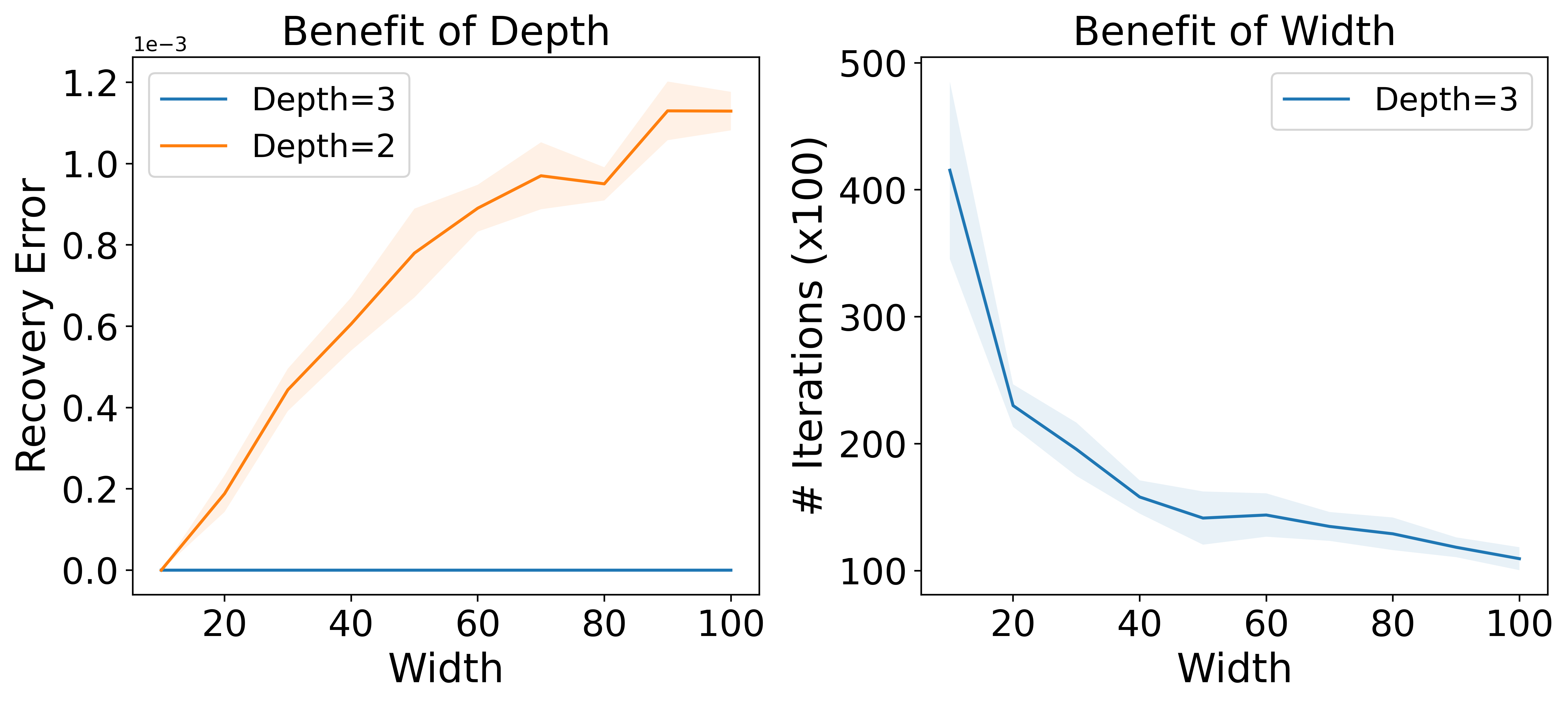
Figure 1: Benefits of depth & width in overparameterized matrix completion with $d=100$, $r^{*}=5$, $\epsilon_{l}=10^{-3}$ and 30% of entries observed. Left: Recovery error vs. width for shallow and deep factorizations. Right: Number of GD iterations to converge to $10^{-10}$ error vs. width. We observe that depth prevents overfitting, while width improves convergence.

Taking the problem of low-rank matrix recovery as an illustrative example, the seminal work of Arora et al. (2019) showed that deeper factorizations better promote low-rank solutions as a function of depth, consequently mitigating overfitting in the overparameterized regime compared to a classical two-layer factorization approach; see Figure 1 (left). On the other hand, increasing the width of each layer substantially reduces the number of iterations to reach the same training error; see Figure 1 (right).

While overparameterization offers remarkable benefits, it also comes with its computational challenges. The significantly increased number of parameters inevitably results in dramatically higher computational costs. This naturally raises a fundamental question: can we attain the benefits of overparameterization with a substantial reduction in computational costs?

In this work, we show that we can achieve this by exploiting low-dimensional structures of data and compressible learning dynamics in the model weights. In the context of low-rank matrix recovery via deep overparameterized factorizations, we discover an interesting phenomenon that for each weight matrix, the learning dynamics only happen within an approximately invariant low-dimensional subspace throughout all iterations. We rigorously prove this for deep matrix factorization, which also allows us to compress the number of training parameters significantly when dealing with deep matrix completion. Consequently, we can construct and train a nearly equivalent, yet much smaller, compressed factorization without sacrificing the advantages of its overparameterized counterpart.

Interestingly, we empirically find that the above phenomenon can also be observed when employing deep overparameterized weight updates for fine-tuning language models; see Figure 2 for an illustration. Therefore, we can adapt our idea of compressing deep matrix factorization to improve language model fine-tuning. For fine-tuning large-scale pretrained language models, recently low-rank adaptation (LoRA) stands out as the most commonly-used technique due to its effectiveness and efficiency (Hu et al., 2021). The basic idea of LoRA is to freeze the pretrained weights and adapt each one to new tasks by adding and optimizing an update in the form of a two-layer low-rank decomposition. Nonetheless, in practical scenarios, selecting the optimal rank of the decomposition can pose a significant challenge. If the rank is not chosen properly, it may lead to overfitting, particularly when we overestimate the rank or when there is limited downstream data available.

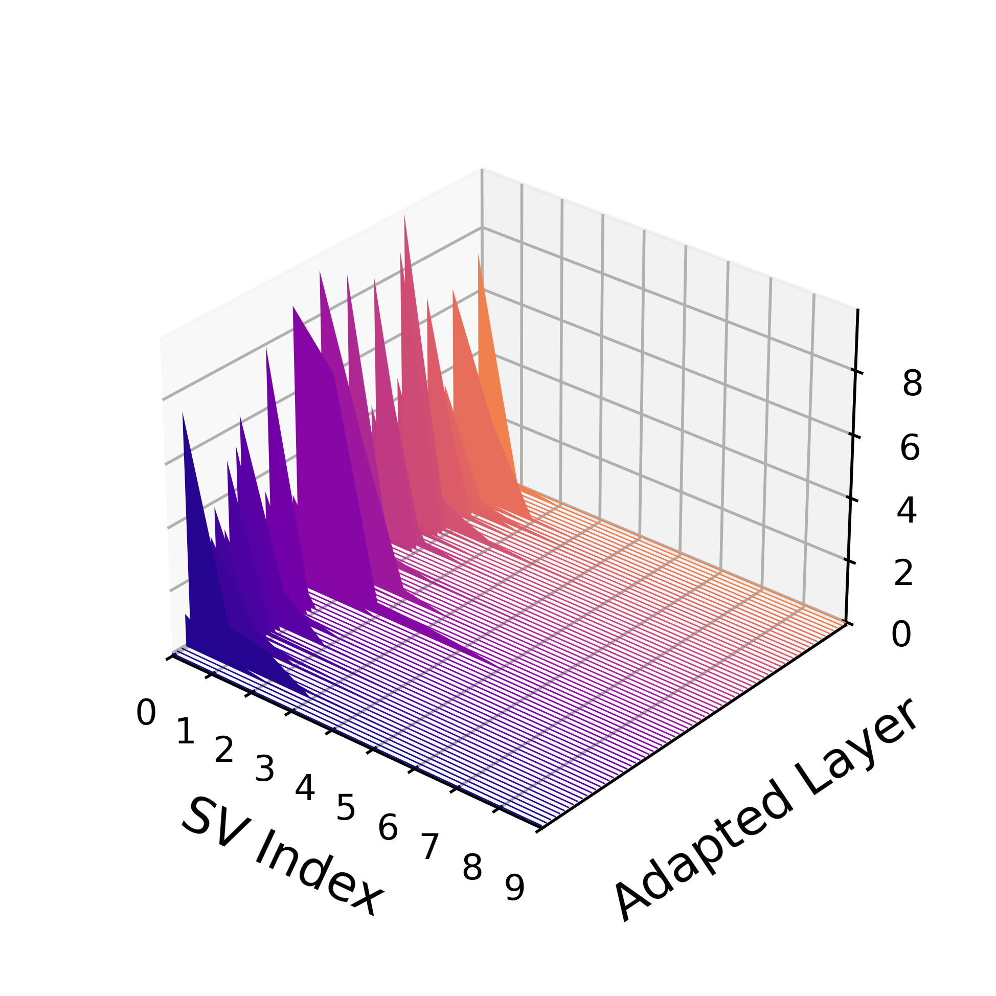
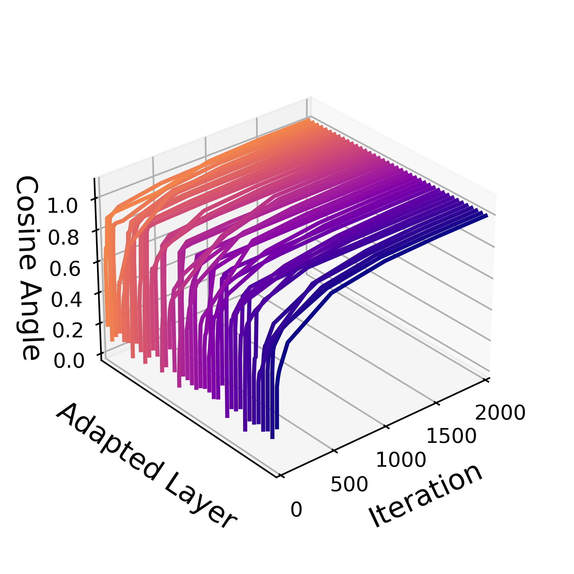
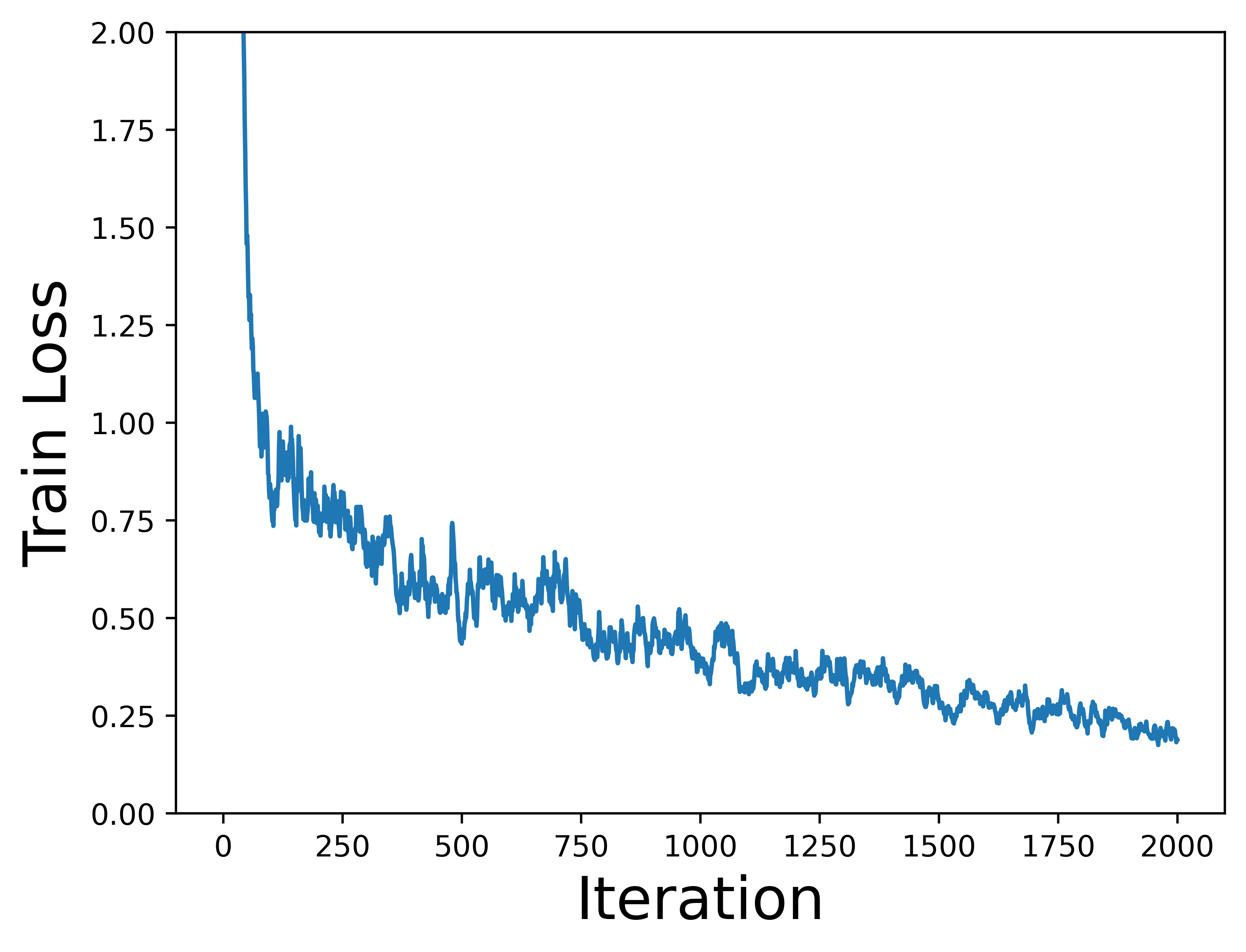
Figure 2: Invariant low-dimensional subspaces in deep overparameterized adaptation of language models. Fine-tuning BERT (Devlin et al., 2019) with deep overparameterized adaptation on the STS-B dataset (Cer et al., 2017). Left: Singular value spectra across all adapted layers at the end of fine-tuning. Middle: Alignment of subspaces formed by top 8 right singular vectors between current adapted weights and final adapted weights throughout training. Right: Training loss continues to decrease in iterations after subspace alignment with final adapted weights. See Section 4 for more details.

We deal with this drawback of LoRA by employing a deep (three-layer) overparameterized factorization for the trainable update, which is constructed and optimized via the compression technique used for deep matrix completion. As such, our new method, which we term as Deep LoRA, enjoys notable advantages over the original LoRA method, namely (i) less overfitting by exploiting depth, and (ii) fewer hyperparameters without rank $r$ and scale $\alpha$ having to be carefully tuned across all layers, all while having a comparable parameter efficiency due to compression.

Contributions.

We summarize our contributions below.

• Practical contributions. We develop efficient compression methods by exploring compressible learning dynamics in overparameterized factorizations. Our method enjoys the benefits of overparameterization while significantly improving its efficiency. We demonstrate the effectiveness not only on deep matrix completion, but also for improving LoRA for language model fine-tuning.

• Theoretical contributions. Our methods are inspired by our theoretical results for deep matrix factorization. Mathematically, we rigorously prove the existence of invariant low-dimensional subspaces throughout gradient descent for each weight matrix, and show how they can constructed in practice.

Related Works

There is a great deal of literature on implicit regularization in the setting of matrix factorization/linear networks (Neyshabur et al., 2015; Gunasekar et al., 2017; Arora et al., 2019; Moroshko et al., 2020; Timor et al., 2023; Ji and Telgarsky, 2019; Gidel et al., 2019; You et al., 2020; Liu et al., 2022), as well as low-rank learning in deep networks (Jaderberg et al., 2014; Sainath et al., 2013; Denil et al., 2013; Khodak et al., 2020; Oymak et al., 2019; Min Kwon et al., 2024; Tarzanagh et al., 2023). Similarly, there is an abundance of work discussing the benefits of overparameterization (Du and Hu, 2019; Arora et al., 2018b; Allen-Zhu et al., 2019b; Arpit and Bengio, 2019).

2 Warm-up Study: Deep Matrix Factorization

Towards gaining theoretical insights into the phenomena in Figure 2, we first build some intuition based on the problem of deep matrix factorization. Under simplified settings, we rigorously unveil the emergence of low-dimensionality and compressibility in gradient descent learning dynamics.

2.1 Basic Setup

Given a low-rank matrix $\bm{\Phi}\in\mathbb{R}^{d_{x}\times d_{y}}$ with $\mbox{rank}(\bm{\Phi})=r^{*}$, we approximate the matrix $\bm{\Phi}$ by an $L$-layer deep overparameterized factorization

$$f(\bm{\Theta}):=\bm{W}_{L}\bm{W}_{L-1}\cdots\bm{W}_{2}\bm{W}_{1}=\bm{W}_{L:1},$$ (1)

where $\bm{\Theta}=(\bm{W}_{l})_{l=1}^{L}$ are the parameters with weights $\bm{W}_{l}\in\mathbb{R}^{d_{l}\times d_{l-1}}$ for $l\in[L]$. We consider the case where the weights are all square $d_{0}=d_{1}=\dots=d_{L}=d$, and learn the parameters $\bm{\Theta}$ by solving

$$\min_{\bm{\Theta}}\ell(\bm{\Theta})=\frac{1}{2}\|f(\bm{\Theta})-\bm{\Phi}\|_{F}^{2}$$ (2)

via gradient descent (GD) from scaled orthogonal initialization, i.e., we initialize parameters $\bm{\Theta}(0)$ such that

$$\bm{W}_{l}(0)\bm{W}_{l}(0)^{\top}=\bm{W}_{l}(0)^{\top}\bm{W}_{l}(0)=\epsilon_{l}^{2}\bm{I}_{d},\;l\in[L]$$ (3)

where $\epsilon_{l}>0$. We assume this for ease of analysis, and believe that our results could hold for arbitrary small initialization. For each weight matrix, the GD iterations can be written as

$$\bm{W}_{l}(t+1)=(1-\eta\lambda)\bm{W}_{l}(t)-\eta\nabla_{\bm{W}_{l}}\ell(\bm{\Theta}(t)),\;l\in[L]$$ (4)

for $t=0,1,2,\dots$, where $\eta>0$ is the learning rate and $\lambda\geq 0$ is an optional weight decay parameter.

2.2 Main Theorem

We show that learning only occurs within an invariant low-dimensional subspace of the weight matrices, whose dimensionality depends on $\mbox{rank}(\bm{\Phi})$.

Figure 3: Evolution of SVD of weight matrices. We visualize the SVD dynamics of the first layer weight matrix of an $L=3$ layer deep matrix factorization for a random matrix with $d=30$, $r^{*}=3$, $\epsilon_{l}=1$ throughout GD without weight decay. Left: Magnitude of the $i$-th singular value $\sigma_{i}(t)$ at iteration $t$. Middle: Angle $\angle(\bm{v}_{i}(t),\bm{v}_{i}(0))$ between the $i$-th right singular vector at iteration $t$ and initialization. Right: Angle $\angle(\bm{u}_{i}(t),\bm{u}_{i}(0))$ between the $i$-th left singular vector at iteration $t$ and initialization.

Theorem 2.1.

Let $\bm{W}_{l}(t)$ satisfy the initialization scheme (3) and updates (4), and suppose $\bm{\Phi}\in\mathbb{R}^{d\times d}$ is at most rank $r$ and let $m:=d-2r>0$. Then there exist orthogonal matrices $(\bm{U}_{l})_{l=1}^{L}\subset\mathcal{O}^{d\times d}$ and $(\bm{V}_{l})_{l=1}^{L}\subset\mathcal{O}^{d\times d}$ (depending only on $\bm{\Theta}(0)$ and $\bm{\Phi}$) satisfying $\bm{V}_{l+1}=\bm{U}_{l}$ for $l\in[L-1]$, such that $\bm{W}_{l}(t)$ admits the decomposition

$$\bm{W}_{l}(t)=\bm{U}_{l}\begin{bmatrix}\widetilde{\bm{W}}_{l}(t)&\bm{0}\\ \bm{0}&\rho_{l}(t)\bm{I}_{m}\end{bmatrix}\bm{V}_{l}^{\top}$$ (5)

for all $l\in[L]$ and $t\geq 0$, where $\widetilde{\bm{W}}_{l}(t)\in\mathbb{R}^{2r\times 2r}$ with $\widetilde{\bm{W}}_{l}(0)=\epsilon_{l}\bm{I}_{2r}$, and

$$\rho_{l}(t)=\rho_{l}(t-1)\cdot(1-\eta\lambda-\eta\cdot\prod_{k\neq l}\rho_{k}^{2}(t-1))$$ (6)

for all $l\in[L]$ and $t\geq 1$ with $\rho_{l}(0)=\epsilon_{l}$.

In the following, we discuss several implications of our result and its relationship to previous work.

• SVD dynamics of weight matrices. The decomposition (5) is closely related to the singular value decomposition (SVD) of $\bm{W}_{l}(t)$. Specifically, let $\bm{U}_{l}=[\bm{U}_{l,1}\ \bm{U}_{l,2}]$, $\bm{V}_{l}=[\bm{V}_{l,1}\ \bm{V}_{l,2}]$, where $\bm{U}_{l,1},\bm{V}_{l,1}\in\mathcal{O}^{d\times 2r}$, $\bm{U}_{l,2},\bm{V}_{l,2}\in\mathcal{O}^{d\times(d-2r)}$. Let $\widetilde{\bm{W}}_{l}(t)=\widetilde{\bm{U}}_{l}(t)\widetilde{\bm{\Sigma}}_{l}(t)\widetilde{\bm{V}}_{l}^{\top}(t)$ be an SVD of $\widetilde{\bm{W}}_{l}(t)$, where $\widetilde{\bm{U}}_{l}(t),\widetilde{\bm{V}}_{l}(t)\in\mathcal{O}^{2r}$ and $\widetilde{\bm{\Sigma}}_{l}(t)\in\mathbb{R}^{2r\times 2r}$ is a diagonal matrix. Then, by (5) we can write $\bm{W}_{l}(t)$ as

  $$\bm{W}_{l}(t)=\begin{bmatrix}\bm{U}_{l,1}\widetilde{\bm{U}}_{l}(t)&\bm{U}_{l,2}\end{bmatrix}\begin{bmatrix}\widetilde{\bm{\Sigma}}_{l}(t)&\bm{0}\\ \bm{0}&\rho(t)\bm{I}_{m}\end{bmatrix}\begin{bmatrix}\bm{V}_{l,1}\widetilde{\bm{V}}_{l}(t)&\bm{V}_{l,2}\end{bmatrix}^{\top}$$

  which is essentially an SVD of $\bm{W}_{l}(t)$ (besides the ordering of singular values). According to this, we can verify that $\rho(t)$ is a (repeated) singular value undergoing minimal changes across iterations illustrated in Figure 3 (left). Additionally, these repeated singular values correspond to invariant subspaces $\bm{U}_{l,2},\bm{V}_{l,2}$ that are stationary throughout GD, as seen in Figure 3 (middle and right).

• Low-rank bias. From (6), we can show under mild assumptions that the GD trajectory for each weight matrix either remains or tends towards a solution with rank at most $2r$. This is true whether we employ implicit or explicit regularization. Indeed, if we use small initialization $\epsilon_{l}\approx 0$ with no weight decay $\lambda=0$, then the fact that $\rho_{l}$ is a decreasing sequence (w.r.t. iteration) implies that the approximate rank of $\bm{W}_{l}(t)$ can be no more than $2r$ throughout the entire trajectory. On the other hand, if we use weight decay with $\lambda>0$, then we have $\rho_{l}(t)\rightarrow 0$ as $t\rightarrow\infty$. This forces $\bm{W}_{l}(t)$ towards a solution of rank at most $2r$ when the training converges. See Section E.2 for a formal statement and proof. This result is consistent with previous findings on low-rank and simplicity bias in deep networks (Huh et al., 2022; Galanti and Poggio, 2022; Li et al., 2020; Chou et al., 2024).

• Comparison to prior arts. In contrast to existing work studying implicit bias of GD towards low-rank solutions (Gunasekar et al., 2017; Arora et al., 2019), our result explicitly shows how GD finds these solutions. Moreover, unlike previous work on implicit bias (Min et al., 2021; Gissin et al., 2019; Arora et al., 2019; Vardi and Shamir, 2021), we also examine the effect of weight decay, which is commonly employed during the training of deep networks. Our analysis is distinct from that of (Saxe et al., 2014, 2019), which studied continuous time dynamics under the special (separable) setting $\bm{W}_{L:1}(0)=\bm{U}\bm{V}^{\top}$ with $\bm{\Phi}=\bm{U}\bm{\Sigma}\bm{V}^{\top}$. In comparison, our result applies to discrete time dynamics and holds for initialization that is agnostic to the target matrix. It should also be noted that our result does not depend on balanced initialization like those in (Arora et al., 2018a), as the initialization scale $\epsilon_{l}$ for each layer can be arbitrarily different from one another.

A sketch of analysis.

We now provide a rough sketch for the beginning of the proof of Theorem 2.1 in the special case of small initialization $\epsilon_{l}=\epsilon\approx 0$ for all $l\in[L]$ and $\lambda=0$, highlighting the construction of the invariant subspace at initialization. The full proof can be found in Section E.1.

Proof sketch.

Since $\epsilon^{L}\approx 0$, from the gradient of $\ell(\bm{\Theta})$ (see Appendix E), we have

$$\bm{G}_{1}:=\nabla_{\bm{W}_{1}}\ell(\bm{\Theta}(0))\approx-\bm{W}_{L:2}^{\top}(0)\bm{\Phi}$$ (7)

implying that the rank of $\bm{G}_{1}$ is (approximately) at most $r$. Now consider the subspace $\mathcal{S}=\mathcal{N}(\bm{G}_{1})\cap\mathcal{N}(\bm{G}_{1}^{\top}\bm{W}_{1}(0))$, where we have $\dim\,\mathcal{S}\geq d-2r$. Then, there exist orthonormal sets $\{\bm{v}_{i}\}_{i=1}^{d-2r}$ and $\{\bm{u}_{i}\}_{i=1}^{d-2r}$ which satisfy $\bm{G}_{1}\bm{v}_{i}=\bm{0}$, $\bm{u}_{i}\propto\bm{W}_{1}(0)\bm{v}_{i}$ and therefore

$$\bm{G}_{1}^{\top}\bm{u}_{i}\propto\bm{G}_{1}^{\top}\bm{W}_{1}(0)\bm{v}_{i}=\bm{0}$$

so along with the orthogonality of $\bm{W}_{1}(0)$, the pairs $(\bm{u}_{i},\bm{v}_{i})$ form singular vector pairs of both $\bm{W}_{1}(0)$ and $\bm{W}_{1}(1)$ simultaneously as they remain unchanged by the gradient update $\bm{G}_{1}$, giving the last $d-2r$ columns of $\bm{V}_{1}$ and $\bm{U}_{1}$ respectively. To see that we can take $\bm{V}_{2}=\bm{U}_{1}$, for instance, we note that

$$\nabla_{\bm{W}_{2}}\ell(\bm{\Theta}(0))\cdot\bm{u}_{i} \approx-\bm{W}_{L:3}^{\top}(0)\bm{\Phi}\bm{W}_{1}^{\top}(0)\bm{u}_{i}$$

$$\propto\bm{W}_{L:3}^{\top}(0)\bm{\Phi}\bm{v}_{i}=\bm{0}$$

by $\eqref{eq:g1}$, showing that $\bm{u}_{i}$ are invariant under gradient updates in the second layer. ∎

2.3 Compression of Overparameterized Factorization

We now show that, as a consequence of Theorem 2.1 and the proof sketch, we can run GD on dramatically fewer parameters to achieve a near identical end-to-end trajectory as the original (full-width) factorization; see Figure 4.

Constructing the “equivalent” compressed factorization.

More specifically, given that $\bm{\Phi}$ is at most rank $r$ and $d-2r>0$, from Theorem 2.1 we observe that

$$\bm{W}_{L:1}(t) =\bm{U}_{L,1}\widetilde{\bm{W}}_{L:1}(t)\bm{V}_{1,1}^{\top}+\left(\prod_{l=1}^{L}\rho_{l}(t)\right)\cdot\bm{U}_{L,2}\bm{V}_{1,2}^{\top}$$

$$\approx\underbrace{\bm{U}_{L,1}\widetilde{\bm{W}}_{L:1}(t)\bm{V}_{1,1}^{\top}}_{=:f_{C}(\widetilde{\bm{\Theta}},\bm{U}_{L,1},\bm{V}_{1,1})},\quad\forall\;t=1,2,\dots,$$ (8)

when we use initialization of small scale (i.e., $(\epsilon_{l})_{l=1}^{L}$ are small). Here, $\widetilde{\bm{W}}_{L:1}=\widetilde{\bm{W}}_{L}\widetilde{\bm{W}}_{L-1}\cdots\widetilde{\bm{W}}_{1}$ with compressed weights $\widetilde{\bm{W}}_{l}\in\mathbb{R}^{2r\times 2r}$. Correspondingly, $f_{C}(\widetilde{\bm{\Theta}},\bm{U}_{L,1},\bm{V}_{1,1})$ denotes the compressed function with compressed parameters $\widetilde{\bm{\Theta}}=(\widetilde{\bm{W}}_{l})_{l=1}^{L}$. As such, we can expect that solving

$$\min_{\widetilde{\bm{\Theta}}}\ell_{C}(\widetilde{\bm{\Theta}})=\frac{1}{2}\|f_{C}(\widetilde{\bm{\Theta}},\bm{U}_{L,1},\bm{V}_{1,1})-\bm{\Phi}\|_{F}^{2}$$ (9)

will approximately give the same solution as (2).

Figure 4: Network compression for deep matrix factorization. Comparison of trajectories for optimizing the original problem (2) vs. the compressed problem (9) with $L=3$, $d=1000$, $r=r^{*}=5$, and $\epsilon_{l}=10^{-3}$. Left: Principal components of end-to-end GD trajectories. Right: Training loss vs. wall-time comparison.

Constructing the factors $(\bm{U}_{l},\bm{V}_{l})_{l=1}^{L}$.

As Theorem 2.1 only showed the existence of $(\bm{U}_{l},\bm{V}_{l})_{l=1}^{L}$, to solve (9) via GD, we need a practical recipe for constructing $(\bm{U}_{l},\bm{V}_{l})_{l=1}^{L}$ efficiently at initialization of small scale $\epsilon_{l}$. This can be achieved based upon our proof sketch in Section 2.2: we compute $\bm{G}_{1}=\nabla_{\bm{W}_{1}}\ell(\bm{\Theta}(0))\in\mathbb{R}^{d\times d}$, find an orthonormal set $\{\bm{v}_{i}\}_{i=1}^{d-2r}$ contained in $\mathcal{S}=\mathcal{N}(\bm{G}_{1})\cap\mathcal{N}(\bm{G}_{1}^{\top}\bm{W}_{1}(0))$, and complete to an orthonormal basis to yield $\bm{V}_{1}$. The remaining $\bm{U}_{l},\bm{V}_{l}$ can then be iteratively constructed via

$$\bm{U}_{l}=\bm{W}_{l}(0)\bm{V}_{l}/\epsilon_{l},\;\bm{V}_{l+1}=\bm{U}_{l},\;l=1,\cdots,L-1,$$

and $\bm{U}_{L}=\bm{W}_{L}(0)\bm{V}_{L}/\epsilon_{L}$. Finally, we take the first $2r$ columns of $\bm{U}_{L}$ and $\bm{V}_{1}$ to yield $\bm{U}_{L,1}$ and $\bm{V}_{1,1}$, respectively. It should be noted that these compressed factors are related to, yet distinct from, spectral initialization, which is well-studied in the literature (Chi et al., 2019; Khodak et al., 2020; Stöger and Soltanolkotabi, 2021). Since $\bm{U}_{l,1},\bm{V}_{l,1}$ are constructed via orthogonal complements to nullspaces involving the gradient, these directions do indeed correlate with the top singular subspaces of $\bm{\Phi}$ in the deep matrix factorization case (although we do not use the singular value information). On the other hand, our approach is more general through the lens of compression, as it can be applied to a given deep overparameterized factorization trained on an arbitrary loss.

Optimization, complexity, and approximation error.

In summary, we can approximately solve the original problem by solving (9) via GD for the compressed parameters $\widetilde{\bm{\Theta}}=(\widetilde{\bm{W}}_{l})_{l=1}^{L}$, starting from small initialization ($\epsilon_{l}\approx 0$). The factors $\bm{U}_{L,1},\bm{V}_{1,1}$ can be efficiently constructed based upon an iterative scheme that we discussed above from the initial weights.

Comparing the parameter counts of the compressed $f_{C}(\widetilde{\bm{\Theta}},\bm{U}_{L,1},\bm{V}_{1,1})$ vs. the original $f(\bm{\Theta})$, we only need to optimize $4L\cdot r^{2}$ parameters compared to the original $L\cdot d^{2}$. Since $r\ll d$, our approach leads to significant improvement in efficiency during GD; see Figure 4 (right). On the other hand, compression requires some additional computation to construct the factors $\bm{U}_{L,1}$ and $\bm{V}_{1,1}$ prior to training, which involves taking a gradient of the first weight in the original factorization followed by an SVD or QR decomposition to compute an orthonormal basis for $\mathcal{S}$. While this requires an additional $O(d^{3})$ compute, this has the same complexity as a single iteration of GD for the original factorization and is therefore a negligible overhead when comparing the two.

Finally, the following result demonstrates that our compression method can achieve an almost identical end-to-end trajectory when we use small initializations; see Figure 4 (left).

Proposition 2.2.

For $r$ such that $m:=d-2r>0$, if we run GD on the compressed weights $\widetilde{\bm{\Theta}}$ as described above for the loss (9), we have

$$\left\|f(\bm{\Theta}(t))-f_{C}(\widetilde{\bm{\Theta}}(t),\bm{U}_{L,1},\bm{V}_{1,1})\right\|_{F}^{2}\leq m\cdot\prod_{l=1}^{L}\epsilon_{l}^{2}$$

for any iterate $t=0,1,2,\cdots$. Here, $\epsilon_{l}$ is the initialization scale for the weight $\bm{W}_{l}(0)$.

The key idea of Proposition 2.2 is that GD is invariant under orthogonal transformations, and each factor $\widetilde{\bm{W}}_{l}$ in the end-to-end factorization in (9) is the result of an orthogonal transformation of $\bm{W}_{l}$. Then, the approximation error $m\cdot\prod_{l=1}^{L}\epsilon_{l}^{2}$ is only due to the approximation we showed in (8). We defer the full proof to Section E.3.

3 Application I: Deep Matrix Completion

In this section, we show that we can generalize our method in Section 2 from vanilla matrix factorization to solving low-rank matrix completion problems (Candes and Recht, 2012; Candès and Tao, 2010; Davenport and Romberg, 2016) via compressed deep factorizations. Given a ground-truth $\bm{\Phi}\in\mathbb{R}^{d\times d}$ with rank $r^{*}\ll d$, the goal of low-rank matrix completion is to recover $\bm{\Phi}$ from only a few number of observations encoded by a mask $\bm{\Omega}\in\{0,1\}^{d\times d}$. Adopting a matrix factorization approach, we minimize the objective

$$\ell_{\mathrm{mc}}(\bm{\Theta})=\frac{1}{2}\|\bm{\Omega}\odot(f(\bm{\Theta})-\bm{\Phi})\|_{F}^{2},$$ (10)

where $f(\bm{\Theta})$ is the deep overparameterized factorization introduced in (1). The problem simplifies to deep matrix factorization (2) that we studied earlier when $\bm{\Omega}=\bm{1}_{d}\bm{1}_{d}^{\top}$ in the full observation case. Additionally, (10) reduces to vanilla (shallow) matrix factorization when $L=2$, whose global optimality and convergence have been widely studied under various settings (Jain et al., 2013; Zheng and Lafferty, 2016; Sun and Luo, 2016; Ge et al., 2016; Bhojanapalli et al., 2016; Ge et al., 2017; Gunasekar et al., 2017; Li et al., 2019; Chi et al., 2019; Li et al., 2018b; Soltanolkotabi et al., 2023; Sun et al., 2018; Zhang et al., 2020; Ding et al., 2021).

Figure 5: Network compression for deep matrix completion. Comparison of trajectories for optimizing the original problem (10) vs. the compressed problem (11) with $\gamma$ discrepant updates ($\gamma=0.01$) and ablating $\gamma$ ($\gamma=0$) with $L=3$, $d=1000$, $r=r^{*}=5$, $\epsilon_{l}=10^{-3}$ and 20% of entries observed. Left: Principal components of end-to-end trajectories of each factorization. Middle: Recovery error vs. iteration comparison. Right: Recovery error vs wall-time comparison.

A double-edged sword of overparameterization.

In practice, the true rank $r^{*}$ is not known – instead, we assume to have an upper bound $r$ of the same order as $r^{*}$, i.e., $r^{*}\leq r\ll d$. Surprisingly, overparameterization has advantages in terms of both depth $L$ and width $r$:

• Benefits of depth: mitigating overfitting. When $r>r^{*}$, it has been demonstrated (Arora et al., 2019) that optimizing deeper factorizations (i.e., $L\geq 3$) generalize better in the low sample regime, while their shallow counterparts overfit; see Figure 1 (left).

• Benefits of width: improving convergence. On the other hand, increasing the width $r$ of the deep factorization beyond $r^{*}$ results in accelerated convergence in terms of iterations, see Figure 1 (right).

However, the advantages of overparameterization come with the challenges of much higher computational costs. For an $L$-layer factorization of (full)-width $d$, we require $O(L\cdot d^{3})$ multiplications per iteration to evaluate gradients and need to store $O(L\cdot d^{2})$ parameters, where $d$ is often very large. Using ideas from Section 2, however, we can obtain the benefits of overparameterization without the extra computational costs.

Compression for deep matrix completion.

Given the similarity between deep matrix factorization and completion (i.e., $\bm{\Omega}=\bm{1}_{d}\bm{1}_{d}^{\top}$ vs arbitrary $\bm{\Omega}$), it seems straightforward to generalize our compression methods in Section 2.3 to deep matrix completion. However, as shown by the orange trace in Figure 5, direct application does not work well, as the compressed factorization’s trajectory diverges from that of the original. This is because the compressed subspaces $\bm{U}_{L,1},\bm{V}_{1,1}\in\mathbb{R}^{d\times 2\widehat{r}}$ computed at the initialization $\bm{\Theta}(0)$ via the gradient

$$\nabla_{\bm{W}_{1}}\ell_{\mathrm{mc}}(\bm{\Theta}(0))\approx-\bm{W}_{L:2}^{\top}(0)[\bm{\Omega}\odot\bm{\Phi}]$$

can be misaligned with the true subspace due to the perturbation by the mask $\bm{\Omega}$.

Nonetheless, this issue can be mitigated by slowly updating $\bm{U}_{L,1},\bm{V}_{1,1}$ during training. Specifically, compared to (9), we minimize

$$\min_{\widetilde{\bm{\Theta}},\bm{U}_{L,1},\bm{V}_{1,1}}\frac{1}{2}\|\bm{\Omega}\odot(f_{C}(\widetilde{\bm{\Theta}},\bm{U}_{L,1},\bm{V}_{1,1})-\bm{\Phi})\|_{F}^{2}$$ (11)

via GD by updating $\widetilde{\bm{\Theta}},\bm{U}_{L,1},\bm{V}_{1,1}$ simultaneously every iteration, with a learning rate $\eta$ on $\widetilde{\bm{\Theta}}$ along with a discrepant learning rate $\gamma\eta$ on $\bm{U}_{L,1},\bm{V}_{1,1}$. Because we update $\bm{U}_{L,1},\bm{V}_{1,1}$ slower than updating $\widetilde{\bm{\Theta}}$, we generally choose $\gamma>0$ to be small and tuned accordingly for the given problem.

As a result, we reduce computational costs to $O((L+d)\cdot r^{2})$ multiplications per iteration for computing gradients, and $O(d\cdot r+L\cdot r^{2})$ parameters. Yet still the trajectory of the deep compressed factorization ultimately aligns with that of the original, while converging roughly $5\times$ faster w.r.t. wall-time, as demonstrated in Figure 5. Moreover, the accelerated convergence induced by the full-width trajectory results in the compressed factorization being $3\times$ faster than randomly initialized factorizations of similar width – see Section D.1 for more details.

4 Application II: Model Fine-tuning

In this section, we show that our compression idea can be further extended to parameter-efficient fine-tuning of pretrained language models, specifically via low-rank adaptation (LoRA) (Hu et al., 2021). In particular, inspired by our approach for deep matrix completion, we propose Deep Low-Rank Adaptation (Deep LoRA), which consistently outperforms vanilla LoRA in the limited sample regime.

4.1 Deep Low-Rank Adaptation (Deep LoRA)

Background on LoRA.

With the ever-growing size of pretrained models and countless downstream tasks, full model fine-tuning is often computationally infeasible. Given a pretrained model whose parameters consist of a collection of dense weight matrices $\{\bm{W}_{0k}\}_{k=1}^{m}\subset\mathbb{R}^{d\times d}$ (e.g., the query/key/value projections of a transformer (Vaswani et al., 2017)), LoRA seeks to adapt each layer to a given task by freezing the pretrained weight $\{\bm{W}_{0k}\}_{k=1}^{m}$ and optimizing an extra trainable low-rank factorization on top. In other words, the fine-tuned weight $\bm{W}_{k}$ is given by

$$\bm{W}_{k}=\bm{W}_{0k}+\frac{\alpha}{r}\bm{W}_{k}^{(2)}\bm{W}_{k}^{(1)}$$

where $\alpha>0$ is a tunable scale parameter and $\bm{W}_{k}^{(2)}\in\mathbb{R}^{d\times r}$, $\bm{W}_{k}^{(1)}\in\mathbb{R}^{r\times d}$ with $r\ll d$, thereby substantially reducing the number of trainable parameters during fine-tuning.

Figure 6: Deep LoRA shows better performance on few shot fine-tuning over vanilla LoRA, with varying numbers of training samples. For each case, we draw $n$ samples at random from STS-B over 20 trials with different seeds, and measure performance on the validation split of each method using the same train set.

Figure 7: Deep LoRA finds lower rank solutions compared to vanilla LoRA. We plot a histogram of numerical ranks for Deep LoRA and vanilla LoRA with $r=8$ after adapting to STS-B with 256 samples. The numerical rank is computed as the number of singular values $\sigma_{i}$ greater than $10^{-8}$ and $d\sigma_{1}\epsilon$ where $\epsilon$ is machine epsilon.

Figure 8: Deep LoRA is more robust to the choice of rank compared to vanilla LoRA. For each choice of rank $r$, we draw 16 samples at random from STS-B over 5 trials with different seeds, and measure performance on the validation split of each method using the same train set.

Proposed method: Deep LoRA.

For vanilla LoRA, if we view adapting each weight matrix of model as an individual low-rank factorization problem, we have demonstrated in previous sections that overparameterization and subsequently compressing factorizations improves generalization with minimal extra computational costs. With this in mind, we can employ a deep overparameterized adaptation of each pretrained weight as

$$\bm{W}_{k}=\bm{W}_{0k}+\underbrace{\bm{W}_{k}^{(L)}\cdots\bm{W}_{k}^{(2)}\bm{W}_{k}^{(1)}}_{=:\Delta\bm{W}_{k}}$$ (12)

where each $\bm{W}_{k}^{(i)}$ is full-width, i.e., $\bm{W}_{k}^{(i)}\in\mathbb{R}^{d\times d}$. Here, $L>0$ is the depth, and typically we choose $L=3$, which is precisely the setting of Figure 2. From the figure, we can see that (i) all the converged weights $\{\Delta\bm{W}_{k}\}_{k=1}^{m}$ are very low-rank (left panel), (ii) the learning dynamics each for each weight approximately stay within the same invariant subspace throughout the iterations (middle panel), and (iii) this happens independent of the training loss decreasing (right panel).

These observations imply that deep overparameterized factorizations in Deep LoRA are highly compressible, so we can apply the compression method from deep matrix completion in Section 3 to compress the learning dynamics for each individual weight for model fine-tuning. Here, the major differences of our compression approach for deep LoRA from that of deep matrix completion is that (i) we have a separate compressed factorization for each layer to be adapted, and (ii) the fine-tuned loss function can be tailored for specific tasks (e.g., the cross-entropy) besides the $\ell_{2}$ loss.

Advantages of Deep LoRA.

Compared to vanilla LoRA, Deep LoRA has clear advantages that we highlight below. More details are provided in Section 4.2.

• Less overfitting in limited data regime. Fine-tuning overparameterized models using LoRA can still result in overfitting in few shot or limited data regime (Sebastian Raschka, 2023). In comparison, the extra depth in (12) of Deep LoRA can help prevent overfitting (see Figure 8), which is similar to deep matrix completion in Figure 1.

• Robustness to the hyperparameter $r$. As shown in Figure 8, by exploiting the intrinsic low-dimensional dynamics in GD via overparameterization in width, our approach is robust to the choice of the rank $r$ in fine-tuning.

Deep LoRA only requires $3r^{2}$ additional trainable parameters for each adapted layer compared to vanilla LoRA, where $r$ is relatively small (e.g., $r=8$).

4.2 More Experimental Details

To evaluate our approach, we use a pretrained BERT (Devlin et al., 2019) base model and apply adaptation on all attention and feedforward weights in the transformer, resulting in 72 adapted layers in total. Unless stated otherwise, we use $r=8$ for both vanilla and Deep LoRA throughout all experiments, in which case Deep LoRA has roughly 0.01% more parameters (with respect to BERT) than vanilla LoRA. We utilize Adam (Kingma and Ba, 2014) as an optimizer for both methods. See Appendix B for more details on the experimental setup.

Table 1: Improvement of Deep LoRA over vanilla LoRA for limited data GLUE fine-tuning. For each task, we draw 1024 samples at random over 10 trials with different seeds, and report the performance gap (with variance) on the validation split between Deep LoRA and vanilla LoRA using the same train set.

	CoLA	MNLI	MRPC	QNLI	QQP
$\Delta$	$+0.090_{\pm 0.002}$	$+0.011_{\pm 0.0005}$	$+0.0042_{\pm 0.001}$	$+0.048_{\pm 0.0009}$	$+0.005_{\pm 0.0002}$

	RTE	SST-2	STS-B	Overall
$\Delta$	$+0.029_{\pm 0.002}$	$+0.019_{\pm 0.0006}$	$+0.018_{\pm 0.00006}$	$+0.028_{\pm 0.002}$

Advantage I: Better generalization with limited data.

We first evaluate our approach on tasks in the GLUE benchmark (Wang et al., 2018), which is a standard benchmark for natural language understanding. To test the performance in a limited data setting, for one given trial of a single task, we randomly sample $1024$ examples from the task data for fine-tuning, a nd compare the difference in performance on the same train set between Deep LoRA and vanilla LoRA on the entire validation split. From the results shown in Table 1, we can see that Deep LoRA delivers significant improvements across most tasks compared to vanilla LoRA, and on average improves performance by nearly 3 points, a notable margin.

This improvement in performance becomes more pronounced in scenarios with severely limited data, such as few-shot settings. Applying the same sampling procedure as in the prior study to the STS-B dataset, we assess both approaches using only $n\in\{16,64,256\}$ training instances. Experiments in Figure 8 illustrate that Deep LoRA consistently surpasses vanilla LoRA across all sample sizes, with the most significant difference observed when $n=16$.

Deep LoRA finds lower rank solutions.

We find that at the end of fine-tuning, Deep LoRA finds lower rank solutions for $\Delta\bm{W}_{k}$ than vanilla LoRA, as shown in Figure 8. In the limited data setting (256 samples), we see that all adapted layers in the vanilla LoRA saturate the constrained numerical rank $r=8$, while most layers in Deep LoRA are perturbed by matrices with numerical ranks between 0 and 4. This suggests that Deep LoRA can adaptively select the appropriate rank for each layer depending on the task. This low-rank bias induces implicit regularization during the fine-tuning process and ultimately prevents overfitting to the task, particularly when only few training samples are available. As a practical consideration, Deep LoRA also requires a fraction of the memory cost to store compared to vanilla LoRA due to the parsimony in adapted weights.

Advantage II: Robustness to choice of rank $r$.

Due to the scarcity of the target training data, choosing the rank $r$ in LoRA is a delicate process – it needs to be large enough to capture the complexity in modeling the downstream task, while small enough to prevent overfitting. The proposed Deep LoRA, on the other hand, avoids catastrophic overfitting as we increase $r$, as demonstrated in Figure 8. This observation mirrors the behavior seen in deep matrix completion, as illustrated in Figure 1. For shallow factorizations, an overestimation of rank $r$ leads to an increase in the generalization error. In contrast, deep factorizations remain resilient to overfitting.

Finally, we show that Deep LoRA outperforms vanilla LoRA for few-shot natural language generation fine-tuning in Appendix C. We also provide an ablation study in Section D.2 on the compression mechanism for Deep LoRA and show that it is crucial for accelerating training.

5 Conclusion & Future Directions

In this work, we have provided an in-depth exploration of low-dimensionality and compressibility in the dynamics of deep overparameterized learning, providing theoretical understandings in the setting of deep matrix factorization and applications to efficient deep matrix completion and language model adaptation. Finally, we outline a couple potential future directions following this work.

Compressibility in non-linear settings.

Although the results on network compression in Section 2 exploit the specific gradient structure of deep matrix factorizations, we believe that our analysis can provide meaningful direction for analyzing the fully non-linear case.

To sketch an idea, consider the setting of Section 2.1 except with a non-linear factorization, i.e., (1) becomes

$$f(\bm{\Theta}):=\bm{W}_{L}\sigma(\bm{W}_{L-1}\cdots\sigma(\bm{W}_{2}\sigma(\bm{W}_{1})))$$ (13)

where $\sigma$ is (for example) the entry-wise ReLU activation. For concreteness, consider the $L=3$ case. The gradient of the loss with respect to, e.g., $\bm{W}_{2}$ in (2) is given by

$$\nabla_{\bm{W}_{2}}\ell(\bm{\Theta})=[h(\bm{W}_{2}\sigma(\bm{W}_{1}))\odot(\bm{W}_{3}^{\top}\bm{E})]\sigma(\bm{W}_{1})^{\top}$$

where $h$ is the entry-wise unit step function and $\bm{E}=f(\bm{\Theta})-\bm{\Phi}$. Comparing this to the gradient in the linear setting (14), there is a great deal of shared structure, with the two main differences being the non-linearity applied to $\bm{W}_{1}$ in the post factor and a projection on the inner term via $h(\bm{W}_{2}\sigma(\bm{W}_{1}))$. However, we still have the low-rank structure of $\bm{W}_{3}^{\top}\bm{E}$, and the zeroing out of certain entries preserves approximate spectral properties of the matrix (Chatterjee, 2015). Moreover, this projection is akin to the masking via $\bm{\Omega}$ as in deep matrix completion from Section 3, for which we do find compressible dynamics. In Figure 9, we plot the singular value spectrum of the above gradient at small initialization, finding that the top $r^{*}$ singular values separate from the rest of the spectrum. This suggests that we may be able to identify a low-dimensional subspace along which we can achieve similar dynamics to the full parameter space.

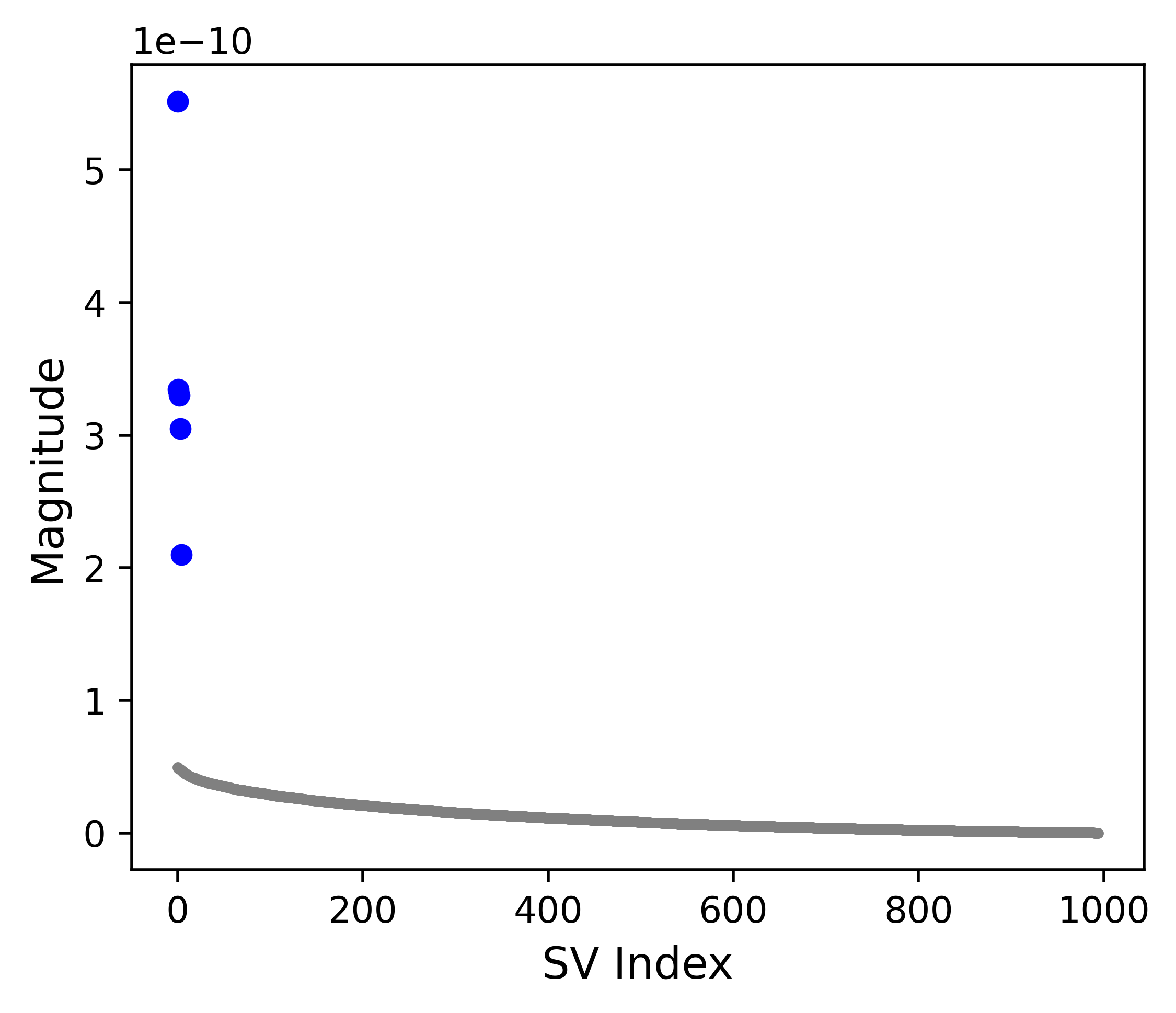
Figure 9: Low-rank gradient of non-linear factorizations at initialization. Singular values spectrum of $\nabla_{\bm{W}_{2}}\ell(\bm{\Theta})$ at initialization for non-linear factorization with $L=3$, $d=1000$, $r^{*}=5$, and $\epsilon_{l}=10^{-3}$. The top 5 singular values separate from the tail of the spectrum.

Extensions to Deep LoRA.

We have demonstrated the efficacy of Deep LoRA for natural language understanding and generation in Section 4 and Appendix C respectively. However, it would be meaningful to evaluate Deep LoRA in other modalities, e.g., diffusion models, where fine-tuning on limited data is commonplace. Moreover, the high degree of alignment at initialization to the final adapted subspaces shown in Figure 2 suggests that SGD (rather than Adam) can be used for the outer factors of Deep LoRA, further reducing memory costs. Finally, exploring the use of second-order methods to accelerate fine-tuning along the rank-$r$ subspace could be a potential improvement.

Implications for representation learning.

The low-rank bias in the end-to-end features of deep networks may have important connections to emergent phenomena in representation learning, such as deep neural collapse (Zhai et al., 2024; Zhou et al., 2022b; Yaras et al., 2022; Wang et al., 2022; Zhou et al., 2022a; Zhu et al., 2021; Beaglehole et al., 2024; Li et al., 2024), whereby the last-layer representations exhibit surprisingly simple structures. Moreover, by uncovering the low-rank evolution of individual weights, we could shed light on more intricate phenomena such as progressive neural collapse (He and Su, 2023; Wang et al., 2023).

 

Appendix

 

Appendix A	Related Works
Appendix B	Experimental Details
Appendix C	Evaluation on Natural Language Generation
Appendix D	Ablating Compression Mechanism
Appendix E	Proofs

In Appendix A, we provide an in-depth discussion of related works. In Appendix B, we provide further details for experiments in Section 4. In Appendix C, we carry out additional experiments for evaluating Deep LoRA for few-shot natural language generation fine-tuning. In Appendix D, we carry out an ablation study for the compression mechanism presented in the main paper, for both deep matrix completion and Deep LoRA. In Appendix E, we provide proofs of all claims from Section 2.

Appendix A Related Works & Future Directions

Implicit regularization.

The first work to theoretically justify implicit regularization in matrix factorization (Gunasekar et al., 2017) was inspired by empirical work that looked into the implicit bias in deep learning (Neyshabur et al., 2015) and made the connection with factorization approaches as deep nets using linear activations. Since then a long line of literature has investigated deep factorizations and their low-rank bias, including (Arora et al., 2019; Moroshko et al., 2020; Timor et al., 2023); in fact there is so much work in this direction that there is already a survey in the Communications of the ACM (Vardi, 2023).

Several older works explicitly imposed low-rank factorization in deep networks (Jaderberg et al., 2014; Sainath et al., 2013) or studied a low-rank factorization of the weights after the learning process (Denil et al., 2013). Newer works along these lines discuss initialization and relationships to regularization (Khodak et al., 2020).

The work in Oymak et al. (2019) also discusses low-rank learning in deep nets, by studying the singular vectors of the Jacobian and arguing that the “information space” or top singular vectors of the Jacobian are learned quickly. Very recent work has shown that the typical factorization of the weights in an attention layer of a transformer into key and query layers has an implicit bias towards low-rank weights (Tarzanagh et al., 2023).

Overparameterization.

There is a sizeable body of work discussing the various benefits of overparameterization in deep learning settings, of which we discuss a few. Du and Hu (2019) demonstrate that width is provably necessary to guarantee convergence of deep linear networks. Arora et al. (2018b) show that overparameterization can result in an implicit acceleration in optimization dynamics for training deep linear networks. Allen-Zhu et al. (2019b) argue that overparameterization plays a fundamental role in rigorously showing that deep networks find global solutions in polynomial time. Arpit and Bengio (2019) shows that depth in ReLU networks improves a certain lower bound on the preservation of variance in information flowing through the network in the form of activations and gradients.

LoRA and its variants.

There is a substantial body of existing work in the realm of parameter efficient fine-tuning – see Xu et al. (2023) for a comprehensive survey. However, the method that has arguably gained the most traction in recent years is LoRA (Hu et al., 2021), in which trainable rank decomposition matrices are added on top of frozen pretrained weights to adapt transformers to downstream tasks. Since then, there has been a plethora of variants. Generalized LoRA (Chavan et al., 2023) proposes a general formulation of LoRA that encapsulates a handful of other parameter efficient adapters. AdaLoRA (Zhang et al., 2022) parameterizes the updates in an SVD-like form and iteratively prunes the inner factor to dynamically control the factorization rank. VeRA (Kopiczko et al., 2024) parameterizes the updates via diagonal adapters which are transformed via random projections that are shared across layers.

The idea of LoRA was initially inspired by the notion of low intrinsic dimension of fine-tuning pretrained models. Intrinsic dimension for an objective was first proposed in Li et al. (2018a), where it was defined to be the minimum dimensionality needed for a random subspace to contain a solution to the objective. Using this idea, Aghajanyan et al. (2021) demonstrated that the objective of fine-tuning a pretrained model has a low intrinsic dimension. Building on this, Zhang et al. (2023) learns the intrinsic subspace of a given fine-tune task from the original parameter trajectory to investigate transferability between these task-specific subspaces.

Appendix B Experimental Details

The pretrained BERT and T5 models are retrieved from the HuggingFace transformers library (Wolf et al., 2019) as google-bert/bert-base-cased and google-t5/t5-base respectively. We choose the best learning rate for each method from $\eta\in\{10^{-5},10^{-4},10^{-3},10^{-2}\}$ on STS-B with 1024 samples, and find that $\eta=10^{-4}$ and $\alpha=8$ works best for vanilla LoRA, while $\eta=10^{-2}$ with $\gamma=10^{-2}$ works best for Deep LoRA (although $\gamma$ can be chosen relatively freely). We tried using a linear decay learning rate but found worse results in the limited data setting for both vanilla and Deep LoRA. We use a maximum sequence length of 128 tokens for all tasks. Vanilla LoRA is initialized in the same fashion as the original paper (i.e., $\bm{W}_{k}^{(2)}$ is initialized to all zeros, $\bm{W}_{k}^{(1)}$ is initialized to be Gaussian with standard deviation 1), whereas Deep LoRA is compressed from a full-width 3-layer factorization with orthogonal initialization of scale $\epsilon_{l}=10^{-3}$. We use a train batch size of 16, and train all models until convergence in train loss, and use the final model checkpoint for evaluation. For generative tasks, we use beam search Freitag and Al-Onaizan (2017) with beam size 4 and maximum generation length of 64. All experiments are carried out on a single NVIDIA Tesla V100 GPU, with time and memory usage reported in Table 2.

Table 2: Comparison of step wall-time and memory usage for vanilla and Deep LoRA.

Method	Iteration Wall-Time (ms)	Memory Usage (GB)
Vanilla LoRA	102	12.526
Deep LoRA	106	12.648

Appendix C Evaluation on Natural Language Generation

In addition to the natural language understanding tasks evaluated in Section 4, we test the effectiveness of Deep LoRA compared to vanilla LoRA for few-shot fine-tuning for natural language generation (NLG), specifically on the E2E dataset (Novikova et al., 2017) with the T5 base model (Raffel et al., 2020). All hyperparameters are as reported in Section 4 and Appendix B. The results are shown in Table 3. We observe significant improvements using Deep LoRA in BLEU (Papineni et al., 2002) and ROUGE (Lin, 2004) scores, with marginally worse results with respect to METEOR (Banerjee and Lavie, 2005) score.

Table 3: Improvement of Deep LoRA over vanilla LoRA for few-shot NLG fine-tuning. On the E2E dataset, we draw 16 samples at random over 10 trials with different seeds, and report the average performance gap on the validation split between Deep LoRA and vanilla LoRA for various metrics using the same train set.

	BLEU	ROUGE-1	ROUGE-2	ROUGE-L	ROUGE-LSUM	METEOR
$\Delta$	$+0.033$	$+0.032$	$+0.056$	$+0.061$	$+0.047$	$-0.00036$

Appendix D Ablating Compression Mechanism

D.1 Deep Matrix Completion

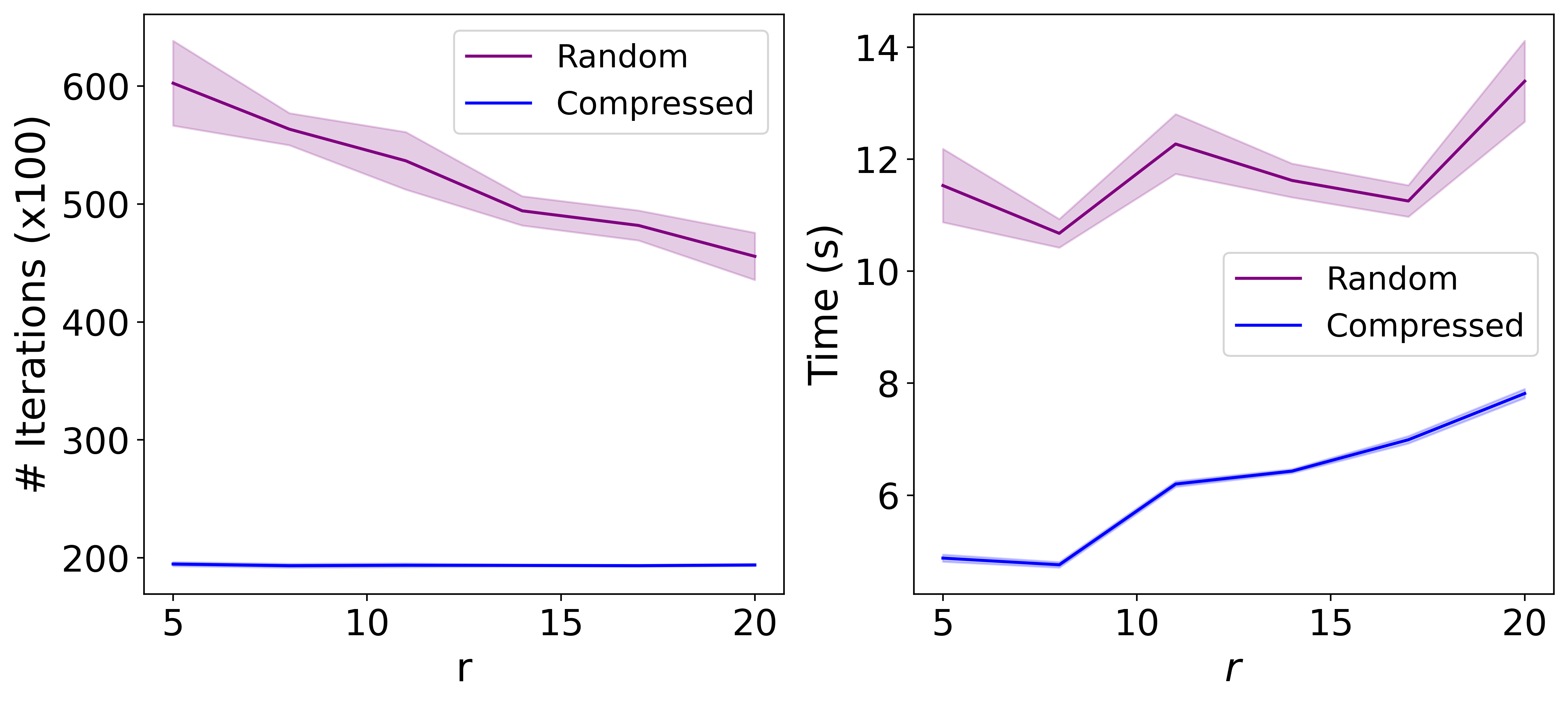
Figure 10: Comparing efficiency of compressed networks vs. randomly initialized narrow networks for deep matrix completion with different overestimated $r$ and $L=3$, $d=1000$, $r^{*}=5$, $\epsilon_{l}=10^{-3}$ and 20% of entries observed. Left: Number of iterations to converge. Right: Wall-time to converge.

We compare the training efficiency of deep $2r$-compressed factorizations (within a wide network of width $d\gg r$) with randomly initialized deep factorizations of width $2r$. As depicted in Figure 10 (left), the compressed factorization requires fewer iterations to reach convergence, and the number of iterations necessary is almost unaffected by $r$. Consequently, training compressed factorizations is considerably more time-efficient than training narrow networks of the same size, provided that $r$ is not significantly larger than $r^{*}$. The distinction between compressed and narrow factorizations underscores the benefits of wide factorizations, as previously demonstrated and discussed in Figure 1 (right), where increasing the width results in faster convergence. However, increasing the width alone also increases computational costs – by employing compression, we can achieve the best of both worlds.

D.2 Deep LoRA

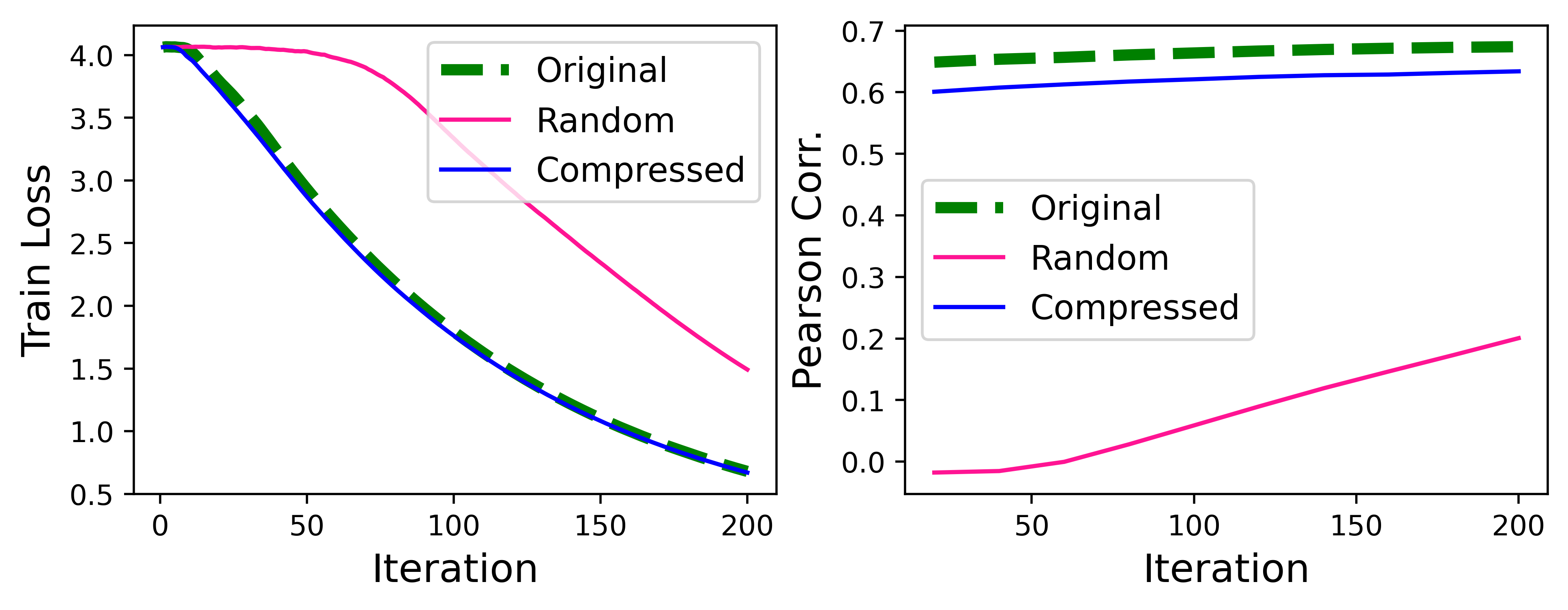
Figure 11: Compression enables faster convergence of Deep LoRA. We compare full-width, compressed, and narrow deep factorizations for adapting to STS-B with 16 samples. Left: Batch train loss vs. iterations. Right: STS-B evaluation metric (Pearson correlation) vs. iterations.

We verify that compression is crucial for the efficiency of Deep LoRA. We compare the performance of three different approaches: (i) Original, where we use a three-layer full-width factorization as in (12), (ii) Compressed, which is the rank-$r$ compression of (12) (a.k.a. Deep LoRA), and (iii) Random, where the $\bm{W}_{k}^{(i)}$ in (12) are initialized randomly with $\bm{W}_{k}^{(2)}\in\mathbb{R}^{r\times r}$. We can see that via compression, Deep LoRA can achieve similar convergence behavior to the original overparameterized factorization with much fewer parameters, while the randomly initialized version takes much longer to train, similar to the result for deep matrix completion in Section D.1.

Appendix E Proofs

The analytic form of the gradient $\nabla_{\bm{\Theta}}\,\ell(\bm{\Theta})$ is given by

$$\nabla_{\bm{W}_{l}}\ell(\bm{\Theta})=\bm{W}_{L:l+1}^{\top}\bm{E}\bm{W}_{l-1:1}^{\top},\;l\in[L]$$ (14)

where $\bm{E}=f(\bm{\Theta})-\bm{\Phi}$, which when substituted into (4) gives the update rules

$$\bm{W}_{l}(t+1)=(1-\eta\lambda)\bm{W}_{l}(t)-\eta\bm{W}_{L:l+1}^{\top}(t)\bm{E}(t)\bm{W}_{l-1:1}^{\top}(t),\;l\in[L]$$ (15)

for $t=0,1,2,\dots$, where $\bm{E}(t)=f(\bm{\Theta}(t))-\bm{\Phi}$.

We first establish the following Lemma E.1 – the claim in Theorem 2.1 then follows in a relatively straightforward manner. We note that all statements quantified by $i$ in this section implicity hold for all $i\in[m]$ (as defined in Theorem 2.1) for the sake of notational brevity.

E.1 Proof of Theorem 2.1

Lemma E.1.

Under the setting of Theorem 2.1, there exist orthonormal sets $\{\bm{u}_{i}^{(l)}\}_{i=1}^{m}\subset\mathbb{R}^{d}$ and $\{\bm{v}_{i}^{(l)}\}_{i=1}^{m}\subset\mathbb{R}^{d}$ for $l\in[L]$ satisfying $\bm{v}_{i}^{(l+1)}=\bm{u}_{i}^{(l)}$ for all $l\in[L-1]$ such that the following hold for all $t\geq 0$:

$$\mathcal{A}(t) :\bm{W}_{l}(t)\bm{v}_{i}^{(l)}=\rho_{l}(t)\bm{u}_{i}^{(l)}\quad \forall l\in[L],$$

$$\mathcal{B}(t) :\bm{W}_{l}^{\top}(t)\bm{u}_{i}^{(l)}=\rho_{l}(t)\bm{v}_{i}^{(l)}\quad \forall l\in[L],$$

$$\mathcal{C}(t) :\bm{\Phi}^{\top}\bm{W}_{L:l+1}(t)\bm{u}_{i}^{(l)}=\bm{0}\quad \forall l\in[L],$$

$$\mathcal{D}(t) :\bm{\Phi}\bm{W}^{\top}_{l-1:1}(t)\bm{v}_{i}^{(l)}=\bm{0}\quad \forall l\in[L],$$

where $\rho_{l}(t)=\rho_{l}(t-1)\cdot(1-\eta\lambda-\eta\cdot\prod_{k\neq l}\rho_{k}(t-1)^{2})$ for all $t\geq 1$ with $\rho_{l}(0)=\epsilon_{l}>0$.

Proof.

Define $\bm{\Psi}:=\bm{W}^{\top}_{L:2}(0)\bm{\Phi}$. Since the rank of $\bm{\Phi}$ is at most $r$, we have that the rank of $\bm{\Psi}\in\mathbb{R}^{d\times d}$ is at most $r$, which implies that $\mathrm{dim}\,\mathcal{N}\left(\bm{\Psi}\right)=\mathrm{dim}\,\mathcal{N}\left(\bm{\Psi}^{\top}\right)\geq d-r$. We define the subspace

$$\mathcal{S}:=\mathcal{N}\left(\bm{\Psi}\right)\cap\mathcal{N}\left(\bm{\Psi}^{\top}\bm{W}_{1}(0)\right)\subset\mathbb{R}^{d}.$$

Since $\bm{W}_{1}(0)\in\mathbb{R}^{d\times d}$ is nonsingular, we have

$$\mathrm{dim}(\mathcal{S})\geq 2(d-r)-d=m.$$

Let $\{\bm{v}_{i}^{(1)}\}_{i=1}^{m}$ denote an orthonormal set contained in $\mathcal{S}$ and set $\bm{u}_{i}^{(1)}:=\bm{W}_{1}(0)\bm{v}_{i}^{(1)}/\epsilon_{1}$, where $\epsilon_{1}>0$ is the scale of $\bm{W}_{1}(0)$ – since $\bm{W}_{1}(0)/\epsilon_{1}$ is orthogonal, $\{\bm{u}_{i}^{(1)}\}_{i=1}^{m}$ is also an orthonormal set. Then we trivially have $\bm{W}_{1}(0)\bm{v}_{i}^{(1)}=\epsilon_{1}\bm{u}_{i}^{(1)}$, which implies $\bm{W}_{1}^{\top}(0)\bm{u}_{i}^{(1)}=\epsilon_{1}\bm{v}_{i}^{(1)}$. It follows from $\bm{v}_{i}^{(1)}\in\mathcal{S}$ that $\bm{\Psi}\bm{v}_{i}^{(1)}=\bm{0}$ and $\bm{\Psi}^{\top}\bm{W}_{1}(0)\bm{v}_{i}^{(1)}=\bm{0}$, which is equivalent to $\bm{W}^{\top}_{L:2}(0)\bm{\Phi}\bm{v}_{i}^{(1)}=\bm{0}$ and $\bm{\Phi}^{\top}\bm{W}_{L:2}(0)\bm{W}_{1}(0)\bm{v}_{i}^{(1)}=\epsilon_{1}\bm{\Phi}^{\top}\bm{W}_{L:2}(0)\bm{u}_{i}^{(1)}=\bm{0}$ respectively. Since $\bm{W}_{L:2}^{\top}(0)$ is full column rank, we further have that $\bm{\Phi}\bm{v}_{i}^{(1)}=\bm{0}$.

Now let $\mathcal{E}(l)$ denote that we have orthonormal sets $\{\bm{u}_{i}^{(l)}\}_{i=1}^{m}$ and $\{\bm{v}_{i}^{(l)}\}_{i=1}^{m}$ satisfying $\bm{W}_{l}(0)\bm{v}_{i}^{(l)}=\epsilon_{l}\bm{u}_{i}^{(l)}$, $\bm{W}_{l}^{\top}(0)\bm{u}_{i}^{(l)}=\epsilon_{l}\bm{v}_{i}^{(l)}$, $\bm{\Phi}^{\top}\bm{W}_{L:l+1}(0)\bm{u}_{i}^{(l)}=\bm{0}$, and $\bm{\Phi}\bm{W}_{l-1:1}^{\top}(0)\bm{v}_{i}^{(l)}=\bm{0}$. From the above arguments, we have that $\mathcal{E}(1)$ holds – now suppose $\mathcal{E}(k)$ holds for some $1\leq k<L$. Set $\bm{v}_{i}^{(k+1)}:=\bm{u}_{i}^{(k)}$ and $\bm{u}_{i}^{(k+1)}:=\bm{W}_{k+1}(0)\bm{v}_{i}^{(k+1)}/\epsilon_{k+1}$. This implies that $\bm{W}_{k+1}(0)\bm{v}_{i}^{(k+1)}=\epsilon_{k+1}\bm{u}_{i}^{(k+1)}$ and $\bm{W}_{k+1}^{\top}(0)\bm{u}_{i}^{(k+1)}=\epsilon_{k+1}\bm{v}_{i}^{(k+1)}$. Moreover, we have

$$\bm{\Phi}^{\top}\bm{W}_{L:(k+1)+1}(0)\bm{u}_{i}^{(k+1)} =\bm{\Phi}^{\top}\bm{W}_{L:k+1}(0)\bm{W}_{k+1}^{\top}(0)\bm{u}_{i}^{(k+1)}/\epsilon_{k+1}^{2}$$

$$=\bm{\Phi}^{\top}\bm{W}_{L:k+1}(0)\bm{v}_{i}^{(k+1)}/\epsilon_{k+1}$$

$$=\bm{\Phi}^{\top}\bm{W}_{L:k+1}(0)\bm{u}_{i}^{(k)}/\epsilon_{k+1}=\bm{0},$$

where the first two equalities follow from orthogonality and $\bm{u}_{i}^{(k+1)}=\bm{W}_{k+1}(0)\bm{v}_{i}^{(k+1)}/\epsilon_{k+1}$, and the last equality is due to $\bm{v}_{i}^{(k+1)}=\bm{u}_{i}^{(k)}$. Similarly, we have

$$\bm{\Phi}\bm{W}_{(k+1)-1:1}^{\top}(0)\bm{v}_{i}^{(k+1)} =\bm{\Phi}\bm{W}_{k-1:1}^{\top}(0)\bm{W}_{k}^{\top}(0)\bm{v}_{i}^{(k+1)}$$

$$=\bm{\Phi}\bm{W}_{k-1:1}^{\top}(0)\bm{W}_{k}^{\top}(0)\bm{u}_{i}^{(k)}$$

$$=\epsilon_{k}\bm{\Phi}\bm{W}_{k-1:1}^{\top}(0)\bm{v}_{i}^{(k)}=\bm{0},$$

where the second equality follows from $\bm{v}_{i}^{(k+1)}=\bm{u}_{i}^{(k)}$ and the third equality is due to $\bm{W}_{k}^{\top}(0)\bm{u}_{i}^{(k)}=\epsilon_{k}\bm{v}_{i}^{(k)}$. Therefore $\mathcal{E}(k+1)$ holds, so we have $\mathcal{E}(l)$ for all $l\in[L]$. As a result, we have shown the base cases $\mathcal{A}(0)$, $\mathcal{B}(0)$, $\mathcal{C}(0)$, and $\mathcal{D}(0)$.

Now we proceed by induction on $t\geq 0$. Suppose that $\mathcal{A}(t)$, $\mathcal{B}(t)$, $\mathcal{C}(t)$, and $\mathcal{D}(t)$ hold for some $t\geq 0$. First, we show $\mathcal{A}(t+1)$ and $\mathcal{B}(t+1)$. We have

$$\bm{W}_{l}(t+1)\bm{v}_{i}^{(l)} =\left[(1-\eta\lambda)\bm{W}_{l}(t)-\eta\bm{W}_{L:l+1}^{\top}(t)\bm{E}(t)\bm{W}_{l-1:1}^{\top}(t)\right]\bm{v}_{i}^{(l)}$$

$$=\left[(1-\eta\lambda)\bm{W}_{l}(t)-\eta\bm{W}_{L:l+1}^{\top}(t)\left(\bm{W}_{L:1}(t)-\bm{\Phi}\right)\bm{W}_{l-1:1}^{\top}(t)\right]\bm{v}_{i}^{(l)}$$

$$=(1-\eta\lambda)\bm{W}_{l}(t)\bm{v}_{i}^{(l)}-\eta\bm{W}_{L:l+1}^{\top}(t)\bm{W}_{L:1}(t)\bm{W}_{l-1:1}^{\top}(t)\bm{v}_{i}^{(l)}$$

$$=(1-\eta\lambda)\bm{W}_{l}(t)\bm{v}_{i}^{(l)}-\eta\cdot(\prod_{k\neq l}\rho_{k}^{2}(t))\bm{W}_{l}(t)\bm{v}_{i}^{(l)}$$

$$=\rho_{l}(t)\cdot(1-\eta\lambda-\eta\cdot\prod_{k\neq l}\rho_{k}^{2}(t))\bm{u}_{i}^{(l)}=\rho_{l}(t+1)\bm{u}_{i}^{(l)}$$

for all $l\in[L]$, where the first equality follows from (15), the second equality follows from definition of $\bm{E}(t)$, the third equality follows from $\mathcal{D}(t)$, and the fourth equality follows from $\mathcal{A}(t)$ and $\mathcal{B}(t)$ applied repeatedly along with $\bm{v}_{i}^{(l+1)}=\bm{u}_{i}^{(l)}$ for all $l\in[L-1]$, proving $\mathcal{A}(t+1)$. Similarly, we have

$$\bm{W}_{l}^{\top}(t+1)\bm{u}_{i}^{(l)} =\left[(1-\eta\lambda)\bm{W}_{l}^{\top}(t)-\eta\bm{W}_{l-1:1}(t)\bm{E}^{\top}(t)\bm{W}_{L:l+1}(t)\right]\bm{u}_{i}^{(l)}$$

$$=\left[(1-\eta\lambda)\bm{W}_{l}^{\top}(t)-\eta\bm{W}_{l-1:1}(t)\bm{\left missing}(\bm{W}_{L:1}^{\top}(t)-\bm{\Phi}^{\top}\right)\bm{W}_{L:l+1}(t)\right]\bm{u}_{i}^{(l)}$$

$$=(1-\eta\lambda)\bm{W}_{l}^{\top}(t)\bm{u}_{i}^{(l)}-\eta\bm{W}_{l-1:1}(t)\bm{W}_{L:1}^{\top}(t)\bm{W}_{L:l+1}(t)\bm{u}_{i}^{(l)}$$

$$=(1-\eta\lambda)\bm{W}_{l}^{\top}(t)\bm{u}_{i}^{(l)}-\eta\cdot(\prod_{k\neq l}\rho_{k}^{2}(t))\bm{W}_{l}^{\top}(t)\bm{u}_{i}^{(l)}$$

$$=\rho_{l}(t)\cdot(1-\eta\lambda-\eta\cdot\prod_{k\neq l}\rho_{k}^{2}(t))\bm{v}_{i}^{(l)}=\rho_{l}(t+1)\bm{v}_{i}^{(l)}$$

for all $l\in[L]$, where the third equality follows from $\mathcal{C}(t)$, and the fourth equality follows from $\mathcal{A}(t)$ and $\mathcal{B}(t)$ applied repeatedly along with $\bm{v}_{i}^{(l+1)}=\bm{u}_{i}^{(l)}$ for all $l\in[L-1]$, proving $\mathcal{B}(t+1)$. Now, we show $\mathcal{C}(t+1)$. For any $k\in[L-1]$, it follows from $\bm{v}_{i}^{(k+1)}=\bm{u}_{i}^{(k)}$ and $\mathcal{A}(t+1)$ that

$$\bm{W}_{k+1}(t+1)\bm{u}_{i}^{(k)}=\bm{W}_{k+1}(t+1)\bm{v}_{i}^{(k+1)}=\rho_{k+1}(t+1)\bm{u}_{i}^{(k+1)}.$$

Repeatedly applying the above equality for $k=l,l+1,\dots,L-1$, we obtain

$$\bm{\Phi}^{\top}\bm{W}_{L:l+1}(t)\bm{u}_{i}^{(l)}=\left[\prod_{k=l}^{L-1}\rho_{k+1}(t)\right]\cdot\bm{\Phi}^{\top}\bm{u}_{i}^{(L)}=\bm{0}$$

which follows from $\mathcal{C}(t)$, proving $\mathcal{C}(t+1)$. Finally, we show $\mathcal{D}(t+1)$. For any $k\in\{2,\dots,L\}$, it follows from $\bm{v}_{i}^{(k)}=\bm{u}_{i}^{(k-1)}$ and $\mathcal{B}(t+1)$ that

$$\bm{W}_{k-1}^{\top}(t+1)\bm{v}_{i}^{(k)}=\bm{W}_{k-1}^{\top}(t+1)\bm{u}_{i}^{(k-1)}=\rho_{k-1}(t+1)\bm{v}_{i}^{(k-1)}.$$

Repeatedly applying the above equality for $k=l,l-1,\dots,2$, we obtain

$$\bm{\Phi}\bm{W}^{\top}_{l-1:1}(t)\bm{v}_{i}^{(l)}=\left[\prod_{k=2}^{l}\rho_{k-1}(t)\right]\cdot\bm{\Phi}\bm{v}_{i}^{(1)}=\bm{0}$$

which follows from $\mathcal{D}(t)$. Thus we have proven $\mathcal{D}(t+1)$, concluding the proof. ∎

Proof of Theorem 2.1.

By $\mathcal{A}(t)$ and $\mathcal{B}(t)$ of Lemma E.1, there exists orthonormal matrices $\{\bm{U}_{l,2}\}_{l=1}^{L}\subset\mathbb{R}^{d\times m}$ and $\{\bm{V}_{l,2}\}_{l=1}^{L}\subset\mathbb{R}^{d\times m}$ for $l\in[L]$ satisfying $\bm{V}_{l+1,2}=\bm{U}_{l,2}$ for all $l\in[L-1]$ as well as

$$\bm{W}_{l}(t)\bm{V}_{l,2}=\rho_{l}(t)\bm{U}_{l,2}\quad\mbox{and}\quad\bm{W}_{l}(t)^{\top}\bm{U}_{l,2}=\rho_{l}(t)\bm{V}_{l,2}$$ (16)

for all $l\in[L]$ and $t\geq 0$, where $\rho_{l}(t)$ satisfies (6) for $t\geq 1$ with $\rho_{l}(0)=\epsilon_{l}$. First, complete $\bm{V}_{1,2}$ to an orthonormal basis for $\mathbb{R}^{d}$ as $\bm{V}_{1}=[\bm{V}_{1,1}\ \bm{V}_{1,2}]$. Then for each $l\in[L-1]$, set $\bm{U}_{l}=[\bm{U}_{l,1}\ \bm{U}_{l,2}]$ where $\bm{U}_{l,1}=\bm{W}_{l}(0)\bm{V}_{l,1}/\epsilon_{l}$ and $\bm{V}_{l+1}=[\bm{V}_{l+1,1}\ \bm{V}_{l+1,2}]$ where $\bm{V}_{l+1,1}=\bm{U}_{l,1}$, and finally set $\bm{U}_{L}=[\bm{U}_{L,1}\ \bm{U}_{L,2}]$ where $\bm{U}_{L,1}=\bm{W}_{L}(0)\bm{V}_{L,1}/\epsilon_{L}$. We note that $\bm{V}_{l+1}=\bm{U}_{l}$ for each $l\in[L-1]$ and $\bm{U}_{l},\bm{V}_{l}$ are orthogonal since $\bm{W}_{l}(0)/\epsilon_{l}$ is orthogonal for all $l\in[L]$. Then we have

$$\bm{U}_{l,1}^{\top}\bm{W}_{l}(t)\bm{V}_{l,2}=\rho_{l}(t)\bm{U}_{l,1}^{\top}\bm{U}_{l,2}=\bm{0}$$ (17)

for all $l\in[L]$ and $t\geq 0$, where the first equality follows from (16). Similarly, we also have

$$\bm{U}_{l,2}^{\top}\bm{W}_{l}(t)\bm{V}_{l,1}=\rho(t)\bm{V}_{l,2}^{\top}\bm{V}_{l,1}=\bm{0}$$ (18)

for all $l\in[L]$ and $t\geq 0$, where the first equality also follows from (16). Therefore, combining (16), (17), and (18) yields

$$\bm{U}_{l}^{\top}\bm{W}_{l}(t)\bm{V}_{l}=\begin{bmatrix}\bm{U}_{l,1}&\bm{U}_{l,2}\end{bmatrix}^{\top}\bm{W}_{l}(t)\begin{bmatrix}\bm{V}_{l,1}&\bm{V}_{l,2}\end{bmatrix}=\begin{bmatrix}\widetilde{\bm{W}}_{l}(t)&\bm{0}\\ \bm{0}&\rho_{l}(t)\bm{I}_{m}\end{bmatrix}$$

for all $l\in[L]$, where $\widetilde{\bm{W}}_{l}(0)=\epsilon_{l}\bm{I}_{2r}$ by construction of $\bm{U}_{l,1}$. This directly implies (5), completing the proof. ∎

E.2 Low-rank bias in Theorem 2.1

Here, we verify the claims following Theorem 2.1 and give a precise characterization of the rate of decay of $\rho_{l}$ as given by (6) and the conditions on learning rate $\eta$ needed to achieve such behavior. These are given in the following lemma.

Lemma E.2.

In the setting of Theorem 2.1, suppose $0<\epsilon_{l}=\epsilon\leq 1$ for all $l\in[L]$ and $0<\eta\leq\frac{1}{\lambda+\epsilon}$. Then for all $t\geq 0$, the updates of $\rho_{l}(t)$ in (6) satisfy $\rho_{l}(t)=\rho(t)$ for some $\rho$, and

$$\epsilon\cdot(1-\eta\cdot(\lambda+\epsilon))^{t}\leq\rho(t)\leq\epsilon\cdot(1-\eta\lambda)^{t}.$$ (19)

Since $\lambda$ and $\epsilon$ are often chose to be small, the above lemma implies that a small learning rate is not required to achieve a low-rank solution. Moreover, by choice of $\eta$, when weight decay is employed (i.e., $\lambda>0$) the above inequality implies that $\rho(t)\rightarrow 0$ as $t\rightarrow\infty$. When $\lambda=0$, we instead have that $\rho$ is bounded by $\epsilon$.

Proof of Lemma E.2.

If $\rho_{l}(0)=\epsilon$ for all $l\in[L]$, it is clear that $\rho_{l}(t)=\rho(t)$ for some $\rho$ for all $t\geq 0$, and the updates take the form

$$\rho(t)=\rho(t-1)\cdot\left[1-\eta\cdot\left(\lambda+\rho(t-1)^{2(L-1)}\right)\right]$$

for each $t\geq 0$. We proceed by induction. For $t=0$, since $\rho(0)=\epsilon$, the claim holds trivially. Now suppose (19) holds for some $t\geq 0$. By choice of $\eta$, we have that $1-\eta\cdot(\lambda+\epsilon)\geq 0$, so $\rho(t)\geq 0$. It then follows that

$$\rho(t+1)=\rho(t)\cdot\left[1-\eta\cdot\left(\lambda+\rho(t)^{2(L-1)}\right)\right]\leq\rho(t)\cdot(1-\eta\lambda)\leq\epsilon\cdot(1-\eta\lambda)^{t+1}$$

by the fact that $\rho(t)\leq\epsilon\cdot(1-\eta\lambda)^{t}$. Next, by choice of $\eta$ and initial condition, we have that $\rho(t)\leq\epsilon$, so that

$$\rho(t+1)=\rho(t)\cdot\left[1-\eta\cdot\left(\lambda+\rho(t)^{2(L-1)}\right)\right]\geq\rho(t)\cdot(1-\eta\cdot(\lambda+\epsilon))\geq\epsilon\cdot(1-\eta\cdot(\lambda+\epsilon))^{t+1}$$

since $\epsilon^{2(L-1)}\leq\epsilon$ by $\epsilon\leq 1$. The claim follows. ∎

E.3 Proof of Proposition 2.2

Proof.

First, it follows from Theorem 2.1 that for any $1\leq i\leq j\leq L$ we have

$$\bm{W}_{j:i}(t)=\bm{U}_{j,1}\widetilde{\bm{W}}_{j:i}(t)\bm{V}_{i,1}^{\top}+(\prod_{k=i}^{j}\rho_{k}(t))\cdot\bm{U}_{j,2}\bm{V}_{i,2}^{\top}$$ (20)

for all $t\geq 0$, where $\bm{U}_{l,1},\bm{V}_{l,1}\in\mathbb{R}^{d\times 2r}$ and $\bm{U}_{l,2},\bm{V}_{l,2}\in\mathbb{R}^{d\times m}$ are the first $2r$ and last $m$ columns of $\bm{U}_{l},\bm{V}_{l}\in\mathbb{R}^{d\times d}$ respectively.

The key claim to be shown here is that $\widehat{\bm{W}}_{l}(t)=\widetilde{\bm{W}}_{l}(t)$ for all $l\in[L]$ and $t\geq 0$. Afterwards, it follows straightforwardly from (20) that

$$\left\|f(\bm{\Theta}(t))-\widehat{f}(\widehat{\bm{\Theta}}(t),\bm{U}_{L,1},\bm{V}_{1,1})\right\|_{F}^{2}$$

$$= \left\|\bm{U}_{L,1}\widetilde{\bm{W}}_{L:1}(t)\bm{V}_{1,1}^{\top}+(\prod_{l=1}^{L}\rho_{l}(t))\cdot\bm{U}_{L,2}\bm{V}_{1,2}^{\top}-\bm{U}_{L,1}\widehat{\bm{W}}_{L:1}(t)\bm{V}_{L,1}^{\top}\right\|_{F}^{2}$$

$$= \left\|\bm{U}_{L,1}(\widetilde{\bm{W}}_{L:1}(t)-\widehat{\bm{W}}_{L:1}(t))\bm{V}_{1,1}^{\top}+(\prod_{l=1}^{L}\rho_{l}(t))\cdot\bm{U}_{L,2}\bm{V}_{1,2}^{\top}\right\|_{F}^{2}=\left\|(\prod_{l=1}^{L}\rho_{l}(t))\cdot\bm{U}_{L,2}\bm{V}_{1,2}^{\top}\right\|_{F}^{2}\leq m\cdot\prod_{l=1}^{L}\epsilon_{l}^{2}.$$

We proceed by induction. For $t=0$, we have that

$$\widehat{\bm{W}}_{l}(0)=\bm{U}_{l,1}^{\top}\bm{W}_{l}(0)\bm{V}_{l,1}=\widetilde{\bm{W}}_{l}(0)$$

for all $l\in[L]$ by (20) and choice of initialization.

Now suppose $\widehat{\bm{W}}_{l}(t)=\widetilde{\bm{W}}_{l}(t)$ for all $l\in[L]$. Comparing

$$\widehat{\bm{W}}_{l}(t+1)=(1-\eta\lambda)\widehat{\bm{W}}_{l}(t)-\eta\nabla_{\widehat{\bm{W}}_{l}}\widehat{\ell}(\widehat{\bm{\Theta}}(t))$$

with

$$\widetilde{\bm{W}}_{l}(t+1) =\bm{U}_{l,1}^{\top}\bm{W}_{l}(t+1)\bm{V}_{l,1}$$

$$=\bm{U}_{l,1}^{\top}\left[(1-\eta\lambda)\bm{W}_{l}(t)-\eta\nabla_{\bm{W}_{l}}\ell(\bm{\Theta}(t))\right]\bm{V}_{l,1}$$

$$=(1-\eta\lambda)\widetilde{\bm{W}}_{l}(t)-\eta\bm{U}_{l,1}^{\top}\nabla_{\bm{W}_{l}}\ell(\bm{\Theta}(t))\bm{V}_{l,1}$$

it suffices to show that

$$\nabla_{\widehat{\bm{W}}_{l}}\widehat{\ell}(\widehat{\bm{\Theta}}(t))=\bm{U}_{l,1}^{\top}\nabla_{\bm{W}_{l}}\ell(\bm{\Theta}(t))\bm{V}_{l,1},\;\forall l\in[L]$$ (21)

to yield $\widehat{\bm{W}}_{l}(t+1)=\widetilde{\bm{W}}_{l}(t+1)$ for all $l\in[L]$. Computing the right hand side of (21), we have

$$\bm{U}_{l,1}^{\top}\nabla_{\bm{W}_{l}}\ell(\bm{\Theta}(t))\bm{V}_{l,1} =\bm{U}_{l,1}^{\top}\bm{W}^{\top}_{L:l+1}(t)(\bm{W}_{L:1}(t)-\bm{\Phi})\bm{W}^{\top}_{l-1:1}(t)\bm{V}_{l,1}$$

$$=(\bm{W}_{L:l+1}(t)\bm{U}_{l,1})^{\top}(\bm{W}_{L:1}(t)-\bm{\Phi})(\bm{V}_{l,1}^{\top}\bm{W}_{l-1:1}(t))^{\top}$$

where

$$\bm{W}_{L:l+1}(t)\bm{U}_{l,1}=\left(\bm{U}_{L,1}\widetilde{\bm{W}}_{L:l+1}(t)\bm{V}_{l+1,1}^{\top}+(\prod_{k=l+1}^{L}\rho_{k}(t))\cdot\bm{U}_{L,2}\bm{V}_{l+1,2}^{\top}\right)\bm{U}_{l,1}=\bm{U}_{L,1}\widetilde{\bm{W}}_{L:l+1}(t)$$

by (20) and the fact that $\bm{U}_{l}=\bm{V}_{l+1}$, and similarly

$$\bm{V}_{l,1}^{\top}\bm{W}_{l-1:1}(t)=\bm{V}_{l,1}^{\top}\left(\bm{U}_{l-1,1}\widetilde{\bm{W}}_{l-1:1}(t)\bm{V}_{1,1}^{\top}+(\prod_{k=1}^{l-1}\rho_{k}(t))\cdot\bm{U}_{l-1,2}\bm{V}_{1,2}^{\top}\right)=\widetilde{\bm{W}}_{l-1:1}(t)\bm{V}_{1,1}^{\top}.$$

We also have that

$$\bm{U}_{L,1}^{\top}(\bm{W}_{L:1}(t)-\bm{\Phi})\bm{V}_{1,1} =\bm{U}_{L,1}^{\top}\left(\bm{U}_{L,1}\widetilde{\bm{W}}_{L:1}(t)\bm{V}_{1,1}^{\top}+(\prod_{k=1}^{L}\rho_{k}(t))\cdot\bm{U}_{L,2}\bm{V}_{1,2}^{\top}-\bm{\Phi}\right)\bm{V}_{1,1}$$

$$=\widetilde{\bm{W}}_{L:1}(t)-\bm{U}_{L,1}^{\top}\bm{\Phi}\bm{V}_{1,1}$$

so putting together the previous four equalities yields

$$\bm{U}_{l,1}^{\top}\nabla_{\bm{W}_{l}}\ell(\bm{\Theta}(t))\bm{V}_{l,1} =(\bm{W}_{L:l+1}(t)\bm{U}_{l,1})^{\top}(\bm{W}_{L:1}(t)-\bm{\Phi})(\bm{V}_{l,1}^{\top}\bm{W}_{l-1:1}(t))^{\top}$$

$$=\widetilde{\bm{W}}_{L:l+1}^{\top}(t)\bm{U}_{L,1}^{\top}(\bm{W}_{L:1}(t)-\bm{\Phi})\bm{V}_{1,1}\widetilde{\bm{W}}^{\top}_{l-1:1}(t)$$

$$=\widetilde{\bm{W}}_{L:l+1}^{\top}(t)(\widetilde{\bm{W}}_{L:1}(t)-\bm{U}_{L,1}^{\top}\bm{\Phi}\bm{V}_{1,1})\widetilde{\bm{W}}^{\top}_{l-1:1}(t).$$

On the other hand, the left hand side of (21) gives

$$\nabla_{\widehat{\bm{W}}_{l}}\widehat{\ell}(\widehat{\bm{\Theta}}(t)) =\widehat{\bm{W}}_{L:l+1}(t)^{\top}\bm{U}_{L,1}^{\top}(\bm{U}_{L,1}\widehat{\bm{W}}_{L:1}(t)\bm{V}_{1,1}^{\top}-\bm{\Phi})\bm{V}_{1,1}\widehat{\bm{W}}_{l-1:1}(t)^{\top}$$

$$=\widehat{\bm{W}}_{L:l+1}(t)^{\top}(\widehat{\bm{W}}_{L:1}(t)-\bm{U}_{L,1}^{\top}\bm{\Phi}\bm{V}_{1,1})\widehat{\bm{W}}_{l-1:1}(t)^{\top}$$

so (21) holds by the fact that $\widehat{\bm{W}}_{l}(t)=\widetilde{\bm{W}}_{l}(t)$ for all $l\in[L]$, completing the proof. ∎

References

- Aghajanyan et al. (2021) Armen Aghajanyan, Sonal Gupta, and Luke Zettlemoyer. Intrinsic dimensionality explains the effectiveness of language model fine-tuning. In Proceedings of the 59th Annual Meeting of the Association for Computational Linguistics and the 11th International Joint Conference on Natural Language Processing (Volume 1: Long Papers), pages 7319–7328, 2021.
- Allen-Zhu et al. (2019a) Zeyuan Allen-Zhu, Yuanzhi Li, and Yingyu Liang. Learning and generalization in overparameterized neural networks, going beyond two layers. Advances in neural information processing systems, 32, 2019a.
- Allen-Zhu et al. (2019b) Zeyuan Allen-Zhu, Yuanzhi Li, and Zhao Song. A convergence theory for deep learning via over-parameterization. In International conference on machine learning, pages 242–252. PMLR, 2019b.
- Arora et al. (2018a) Sanjeev Arora, Nadav Cohen, Noah Golowich, and Wei Hu. A convergence analysis of gradient descent for deep linear neural networks. In International Conference on Learning Representations, 2018a.
- Arora et al. (2018b) Sanjeev Arora, Nadav Cohen, and Elad Hazan. On the optimization of deep networks: Implicit acceleration by overparameterization. In International Conference on Machine Learning, pages 244–253. PMLR, 2018b.
- Arora et al. (2019) Sanjeev Arora, Nadav Cohen, Wei Hu, and Yuping Luo. Implicit regularization in deep matrix factorization. Advances in Neural Information Processing Systems, 32, 2019.
- Arpit and Bengio (2019) Devansh Arpit and Yoshua Bengio. The benefits of over-parameterization at initialization in deep relu networks. arXiv preprint arXiv:1901.03611, 2019.
- Banerjee and Lavie (2005) Satanjeev Banerjee and Alon Lavie. METEOR: An automatic metric for MT evaluation with improved correlation with human judgments. In Proceedings of the ACL Workshop on Intrinsic and Extrinsic Evaluation Measures for Machine Translation and/or Summarization, pages 65–72, Ann Arbor, Michigan, June 2005. Association for Computational Linguistics. URL https://www.aclweb.org/anthology/W05-0909.
- Beaglehole et al. (2024) Daniel Beaglehole, Peter Súkeník, Marco Mondelli, and Mikhail Belkin. Average gradient outer product as a mechanism for deep neural collapse. arXiv preprint arXiv:2402.13728, 2024.
- Bhojanapalli et al. (2016) Srinadh Bhojanapalli, Behnam Neyshabur, and Nati Srebro. Global optimality of local search for low rank matrix recovery. Advances in Neural Information Processing Systems, 29, 2016.
- Brown et al. (2020) Tom Brown, Benjamin Mann, Nick Ryder, Melanie Subbiah, Jared D Kaplan, Prafulla Dhariwal, Arvind Neelakantan, Pranav Shyam, Girish Sastry, Amanda Askell, et al. Language models are few-shot learners. Advances in neural information processing systems, 33:1877–1901, 2020.
- Buhai et al. (2020) Rares-Darius Buhai, Yoni Halpern, Yoon Kim, Andrej Risteski, and David Sontag. Empirical study of the benefits of overparameterization in learning latent variable models. In International Conference on Machine Learning, pages 1211–1219. PMLR, 2020.
- Candes and Recht (2012) Emmanuel Candes and Benjamin Recht. Exact matrix completion via convex optimization. Communications of the ACM, 55(6):111–119, 2012.
- Candès and Tao (2010) Emmanuel J Candès and Terence Tao. The power of convex relaxation: Near-optimal matrix completion. IEEE Transactions on Information Theory, 56(5):2053–2080, 2010.
- Cer et al. (2017) Daniel Cer, Mona Diab, Eneko Agirre, Inigo Lopez-Gazpio, and Lucia Specia. Semeval-2017 task 1: Semantic textual similarity multilingual and crosslingual focused evaluation. In Proceedings of the 11th International Workshop on Semantic Evaluation (SemEval-2017). Association for Computational Linguistics, 2017.
- Chatterjee (2015) Sourav Chatterjee. Matrix estimation by universal singular value thresholding. The Annals of Statistics, 43(1):177–214, 2015.
- Chavan et al. (2023) Arnav Chavan, Zhuang Liu, Deepak Gupta, Eric Xing, and Zhiqiang Shen. One-for-all: Generalized lora for parameter-efficient fine-tuning. arXiv preprint arXiv:2306.07967, 2023.
- Chi et al. (2019) Yuejie Chi, Yue M Lu, and Yuxin Chen. Nonconvex optimization meets low-rank matrix factorization: An overview. IEEE Transactions on Signal Processing, 67(20):5239–5269, 2019.
- Chou et al. (2024) Hung-Hsu Chou, Carsten Gieshoff, Johannes Maly, and Holger Rauhut. Gradient descent for deep matrix factorization: Dynamics and implicit bias towards low rank. Applied and Computational Harmonic Analysis, 68:101595, 2024.
- Dalton and Deshmane (1991) Jeff Dalton and Atul Deshmane. Artificial neural networks. IEEE Potentials, 10(2):33–36, 1991.
- Davenport and Romberg (2016) Mark A Davenport and Justin Romberg. An overview of low-rank matrix recovery from incomplete observations. IEEE Journal of Selected Topics in Signal Processing, 10(4):608–622, 2016.
- Denil et al. (2013) Misha Denil, Babak Shakibi, Laurent Dinh, Marc’Aurelio Ranzato, and Nando De Freitas. Predicting parameters in deep learning. Advances in neural information processing systems, 26, 2013.
- Devlin et al. (2019) Jacob Devlin, Ming-Wei Chang, Kenton Lee, and Kristina Toutanova. Bert: Pre-training of deep bidirectional transformers for language understanding. In Proceedings of the 2019 Conference of the North American Chapter of the Association for Computational Linguistics: Human Language Technologies, Volume 1 (Long and Short Papers), pages 4171–4186, 2019.
- Ding et al. (2021) Lijun Ding, Liwei Jiang, Yudong Chen, Qing Qu, and Zhihui Zhu. Rank overspecified robust matrix recovery: Subgradient method and exact recovery. Advances in Neural Information Processing Systems, 34:26767–26778, 2021.
- Du and Hu (2019) Simon Du and Wei Hu. Width provably matters in optimization for deep linear neural networks. In International Conference on Machine Learning, pages 1655–1664. PMLR, 2019.
- Freitag and Al-Onaizan (2017) Markus Freitag and Yaser Al-Onaizan. Beam search strategies for neural machine translation. In Proceedings of the First Workshop on Neural Machine Translation, pages 56–60, 2017.
- Galanti and Poggio (2022) Tomer Galanti and Tomaso Poggio. Sgd noise and implicit low-rank bias in deep neural networks. Technical report, Center for Brains, Minds and Machines (CBMM), 2022.
- Ge et al. (2016) Rong Ge, Jason D Lee, and Tengyu Ma. Matrix completion has no spurious local minimum. Advances in neural information processing systems, 29, 2016.
- Ge et al. (2017) Rong Ge, Chi Jin, and Yi Zheng. No spurious local minima in nonconvex low rank problems: A unified geometric analysis. In International Conference on Machine Learning, pages 1233–1242. PMLR, 2017.
- Gidel et al. (2019) Gauthier Gidel, Francis Bach, and Simon Lacoste-Julien. Implicit regularization of discrete gradient dynamics in linear neural networks. Advances in Neural Information Processing Systems, 32, 2019.
- Gissin et al. (2019) Daniel Gissin, Shai Shalev-Shwartz, and Amit Daniely. The implicit bias of depth: How incremental learning drives generalization. In International Conference on Learning Representations, 2019.
- Gunasekar et al. (2017) Suriya Gunasekar, Blake E Woodworth, Srinadh Bhojanapalli, Behnam Neyshabur, and Nati Srebro. Implicit regularization in matrix factorization. Advances in neural information processing systems, 30, 2017.
- He and Su (2023) Hangfeng He and Weijie J Su. A law of data separation in deep learning. Proceedings of the National Academy of Sciences, 120(36):e2221704120, 2023.
- Hu et al. (2021) Edward J Hu, Phillip Wallis, Zeyuan Allen-Zhu, Yuanzhi Li, Shean Wang, Lu Wang, Weizhu Chen, et al. Lora: Low-rank adaptation of large language models. In International Conference on Learning Representations, 2021.
- Huh et al. (2022) Minyoung Huh, Hossein Mobahi, Richard Zhang, Brian Cheung, Pulkit Agrawal, and Phillip Isola. The low-rank simplicity bias in deep networks. Transactions on Machine Learning Research, 2022.
- Jaderberg et al. (2014) Max Jaderberg, Andrea Vedaldi, and Andrew Zisserman. Speeding up convolutional neural networks with low rank expansions. In Proceedings of the British Machine Vision Conference 2014. British Machine Vision Association, 2014.
- Jain et al. (2013) Prateek Jain, Praneeth Netrapalli, and Sujay Sanghavi. Low-rank matrix completion using alternating minimization. In Proceedings of the forty-fifth annual ACM symposium on Theory of computing, pages 665–674, 2013.
- Ji and Telgarsky (2019) Ziwei Ji and Matus Telgarsky. Gradient descent aligns the layers of deep linear networks. In 7th International Conference on Learning Representations, ICLR 2019, 2019.
- Kaplan et al. (2020) Jared Kaplan, Sam McCandlish, Tom Henighan, Tom B Brown, Benjamin Chess, Rewon Child, Scott Gray, Alec Radford, Jeffrey Wu, and Dario Amodei. Scaling laws for neural language models. arXiv preprint arXiv:2001.08361, 2020.
- Khodak et al. (2020) Mikhail Khodak, Neil A Tenenholtz, Lester Mackey, and Nicolo Fusi. Initialization and regularization of factorized neural layers. In International Conference on Learning Representations, 2020.
- Kingma and Ba (2014) Diederik P Kingma and Jimmy Ba. Adam: A method for stochastic optimization. arXiv preprint arXiv:1412.6980, 2014.
- Kopiczko et al. (2024) Dawid Jan Kopiczko, Tijmen Blankevoort, and Yuki M Asano. VeRA: Vector-based random matrix adaptation. In The Twelfth International Conference on Learning Representations, 2024. URL https://openreview.net/forum?id=NjNfLdxr3A.
- Li et al. (2018a) Chunyuan Li, Heerad Farkhoor, Rosanne Liu, and Jason Yosinski. Measuring the intrinsic dimension of objective landscapes. In International Conference on Learning Representations, 2018a.
- Li et al. (2024) Pengyu Li, Xiao Li, Yutong Wang, and Qing Qu. Neural collapse in multi-label learning with pick-all-label loss. In Forty-first International Conference on Machine Learning, 2024.
- Li et al. (2019) Qiuwei Li, Zhihui Zhu, and Gongguo Tang. The non-convex geometry of low-rank matrix optimization. Information and Inference: A Journal of the IMA, 8(1):51–96, 2019.
- Li et al. (2018b) Yuanzhi Li, Tengyu Ma, and Hongyang Zhang. Algorithmic regularization in over-parameterized matrix sensing and neural networks with quadratic activations. In Conference On Learning Theory, pages 2–47. PMLR, 2018b.
- Li et al. (2020) Zhiyuan Li, Yuping Luo, and Kaifeng Lyu. Towards resolving the implicit bias of gradient descent for matrix factorization: Greedy low-rank learning. In International Conference on Learning Representations, 2020.
- Lin (2004) Chin-Yew Lin. ROUGE: A package for automatic evaluation of summaries. In Text Summarization Branches Out, pages 74–81, Barcelona, Spain, July 2004. Association for Computational Linguistics. URL https://www.aclweb.org/anthology/W04-1013.
- Liu et al. (2022) Sheng Liu, Zhihui Zhu, Qing Qu, and Chong You. Robust training under label noise by over-parameterization. In International Conference on Machine Learning, pages 14153–14172. PMLR, 2022.
- Min et al. (2021) Hancheng Min, Salma Tarmoun, Rene Vidal, and Enrique Mallada. On the explicit role of initialization on the convergence and implicit bias of overparametrized linear networks. In International Conference on Machine Learning, pages 7760–7768. PMLR, 2021.
- Min Kwon et al. (2024) Soo Min Kwon, Zekai Zhang, Dogyoon Song, Laura Balzano, and Qing Qu. Efficient low-dimensional compression of overparameterized models. In Sanjoy Dasgupta, Stephan Mandt, and Yingzhen Li, editors, Proceedings of The 27th International Conference on Artificial Intelligence and Statistics, volume 238 of Proceedings of Machine Learning Research, pages 1009–1017. PMLR, 02–04 May 2024.
- Moroshko et al. (2020) Edward Moroshko, Blake E Woodworth, Suriya Gunasekar, Jason D Lee, Nati Srebro, and Daniel Soudry. Implicit bias in deep linear classification: Initialization scale vs training accuracy. Advances in neural information processing systems, 33:22182–22193, 2020.
- Neyshabur et al. (2015) Behnam Neyshabur, Ryota Tomioka, and Nathan Srebro. In search of the real inductive bias: On the role of implicit regularization in deep learning. In Workshop at International Conference of Learning Represeatations, 2015.
- Novikova et al. (2017) Jekaterina Novikova, Ondřej Dušek, and Verena Rieser. The e2e dataset: New challenges for end-to-end generation. In Proceedings of the 18th Annual SIGdial Meeting on Discourse and Dialogue, pages 201–206, 2017.
- Oymak et al. (2019) Samet Oymak, Zalan Fabian, Mingchen Li, and Mahdi Soltanolkotabi. Generalization guarantees for neural networks via harnessing the low-rank structure of the jacobian,. In ICML Workshop on Generalization in Deep Networks, 2019. Long version at https://arxiv.org/abs/1906.05392.
- Papineni et al. (2002) Kishore Papineni, Salim Roukos, Todd Ward, and Wei jing Zhu. Bleu: a method for automatic evaluation of machine translation. pages 311–318, 2002.
- Radford et al. (2019) Alec Radford, Jeffrey Wu, Rewon Child, David Luan, Dario Amodei, Ilya Sutskever, et al. Language models are unsupervised multitask learners. OpenAI blog, 1(8):9, 2019.
- Raffel et al. (2020) Colin Raffel, Noam Shazeer, Adam Roberts, Katherine Lee, Sharan Narang, Michael Matena, Yanqi Zhou, Wei Li, and Peter J Liu. Exploring the limits of transfer learning with a unified text-to-text transformer. Journal of machine learning research, 21(140):1–67, 2020.
- Sainath et al. (2013) Tara N Sainath, Brian Kingsbury, Vikas Sindhwani, Ebru Arisoy, and Bhuvana Ramabhadran. Low-rank matrix factorization for deep neural network training with high-dimensional output targets. In 2013 IEEE international conference on acoustics, speech and signal processing, pages 6655–6659. IEEE, 2013.
- Saxe et al. (2014) A Saxe, J McClelland, and S Ganguli. Exact solutions to the nonlinear dynamics of learning in deep linear neural networks. In Proceedings of the International Conference on Learning Represenatations 2014. International Conference on Learning Represenatations 2014, 2014.
- Saxe et al. (2019) Andrew M Saxe, James L McClelland, and Surya Ganguli. A mathematical theory of semantic development in deep neural networks. Proceedings of the National Academy of Sciences, 116(23):11537–11546, 2019.
- Sebastian Raschka (2023) PhD Sebastian Raschka. Practical tips for finetuning llms using lora (low-rank adaptation), Nov 2023. URL https://magazine.sebastianraschka.com/p/practical-tips-for-finetuning-llms.
- Soltanolkotabi et al. (2023) Mahdi Soltanolkotabi, Dominik Stöger, and Changzhi Xie. Implicit balancing and regularization: Generalization and convergence guarantees for overparameterized asymmetric matrix sensing. In The Thirty Sixth Annual Conference on Learning Theory, pages 5140–5142. PMLR, 2023.
- Stöger and Soltanolkotabi (2021) Dominik Stöger and Mahdi Soltanolkotabi. Small random initialization is akin to spectral learning: Optimization and generalization guarantees for overparameterized low-rank matrix reconstruction. Advances in Neural Information Processing Systems, 34:23831–23843, 2021.
- Sun et al. (2018) Ju Sun, Qing Qu, and John Wright. A geometric analysis of phase retrieval. Foundations of Computational Mathematics, 18:1131–1198, 2018.
- Sun and Luo (2016) Ruoyu Sun and Zhi-Quan Luo. Guaranteed matrix completion via non-convex factorization. IEEE Transactions on Information Theory, 62(11):6535–6579, 2016.
- Tarzanagh et al. (2023) Davoud Ataee Tarzanagh, Yingcong Li, Christos Thrampoulidis, and Samet Oymak. Transformers as support vector machines. In NeurIPS 2023 Workshop on Mathematics of Modern Machine Learning, 2023.
- Timor et al. (2023) Nadav Timor, Gal Vardi, and Ohad Shamir. Implicit regularization towards rank minimization in relu networks. In International Conference on Algorithmic Learning Theory, pages 1429–1459. PMLR, 2023.
- Vardi (2023) Gal Vardi. On the implicit bias in deep-learning algorithms. Communications of the ACM, 66(6):86–93, 2023.
- Vardi and Shamir (2021) Gal Vardi and Ohad Shamir. Implicit regularization in relu networks with the square loss. In Conference on Learning Theory, pages 4224–4258. PMLR, 2021.
- Vaswani et al. (2017) Ashish Vaswani, Noam Shazeer, Niki Parmar, Jakob Uszkoreit, Llion Jones, Aidan N Gomez, Łukasz Kaiser, and Illia Polosukhin. Attention is all you need. Advances in neural information processing systems, 30, 2017.
- Wang et al. (2018) Alex Wang, Amanpreet Singh, Julian Michael, Felix Hill, Omer Levy, and Samuel R Bowman. Glue: A multi-task benchmark and analysis platform for natural language understanding. In International Conference on Learning Representations, 2018.
- Wang et al. (2022) Peng Wang, Huikang Liu, Can Yaras, Laura Balzano, and Qing Qu. Linear convergence analysis of neural collapse with unconstrained features. In OPT 2022: Optimization for Machine Learning (NeurIPS 2022 Workshop), 2022.
- Wang et al. (2023) Peng Wang, Xiao Li, Can Yaras, Zhihui Zhu, Laura Balzano, Wei Hu, and Qing Qu. Understanding deep representation learning via layerwise feature compression and discrimination. arXiv preprint arXiv:2311.02960, 2023.
- Wolf et al. (2019) Thomas Wolf, Lysandre Debut, Victor Sanh, Julien Chaumond, Clement Delangue, Anthony Moi, Pierric Cistac, Tim Rault, Rémi Louf, Morgan Funtowicz, et al. Huggingface’s transformers: State-of-the-art natural language processing. arXiv preprint arXiv:1910.03771, 2019.
- Wu et al. (2017) Lei Wu, Zhanxing Zhu, et al. Towards understanding generalization of deep learning: Perspective of loss landscapes. arXiv preprint arXiv:1706.10239, 2017.
- Xu et al. (2018) Ji Xu, Daniel J Hsu, and Arian Maleki. Benefits of over-parameterization with em. Advances in Neural Information Processing Systems, 31, 2018.
- Xu et al. (2023) Lingling Xu, Haoran Xie, Si-Zhao Joe Qin, Xiaohui Tao, and Fu Lee Wang. Parameter-efficient fine-tuning methods for pretrained language models: A critical review and assessment. arXiv preprint arXiv:2312.12148, 2023.
- Yaras et al. (2022) Can Yaras, Peng Wang, Zhihui Zhu, Laura Balzano, and Qing Qu. Neural collapse with normalized features: A geometric analysis over the riemannian manifold. Advances in neural information processing systems, 35:11547–11560, 2022.
- You et al. (2020) Chong You, Zhihui Zhu, Qing Qu, and Yi Ma. Robust recovery via implicit bias of discrepant learning rates for double over-parameterization. In Advances in Neural Information Processing Systems, 2020.
- Zhai et al. (2024) Yuexiang Zhai, Shengbang Tong, Xiao Li, Mu Cai, Qing Qu, Yong Jae Lee, and Yi Ma. Investigating the catastrophic forgetting in multimodal large language model fine-tuning. In Conference on Parsimony and Learning, pages 202–227. PMLR, 2024.
- Zhang et al. (2021) Chiyuan Zhang, Samy Bengio, Moritz Hardt, Benjamin Recht, and Oriol Vinyals. Understanding deep learning (still) requires rethinking generalization. Communications of the ACM, 64(3):107–115, 2021.
- Zhang et al. (2022) Qingru Zhang, Minshuo Chen, Alexander Bukharin, Pengcheng He, Yu Cheng, Weizhu Chen, and Tuo Zhao. Adaptive budget allocation for parameter-efficient fine-tuning. In The Eleventh International Conference on Learning Representations, 2022.
- Zhang et al. (2020) Yuqian Zhang, Qing Qu, and John Wright. From symmetry to geometry: Tractable nonconvex problems. arXiv preprint arXiv:2007.06753, 2020.
- Zhang et al. (2023) Zhong Zhang, Bang Liu, and Junming Shao. Fine-tuning happens in tiny subspaces: Exploring intrinsic task-specific subspaces of pre-trained language models. In Proceedings of the 61st Annual Meeting of the Association for Computational Linguistics (Volume 1: Long Papers), pages 1701–1713, 2023.
- Zheng and Lafferty (2016) Qinqing Zheng and John Lafferty. Convergence analysis for rectangular matrix completion using burer-monteiro factorization and gradient descent. arXiv preprint arXiv:1605.07051, 2016.
- Zhou et al. (2022a) Jinxin Zhou, Xiao Li, Tianyu Ding, Chong You, Qing Qu, and Zhihui Zhu. On the optimization landscape of neural collapse under mse loss: Global optimality with unconstrained features. In International Conference on Machine Learning, pages 27179–27202. PMLR, 2022a.
- Zhou et al. (2022b) Jinxin Zhou, Chong You, Xiao Li, Kangning Liu, Sheng Liu, Qing Qu, and Zhihui Zhu. Are all losses created equal: A neural collapse perspective. Advances in Neural Information Processing Systems, 35:31697–31710, 2022b.
- Zhu et al. (2021) Zhihui Zhu, Tianyu Ding, Jinxin Zhou, Xiao Li, Chong You, Jeremias Sulam, and Qing Qu. A geometric analysis of neural collapse with unconstrained features. Advances in Neural Information Processing Systems, 34:29820–29834, 2021.