Monte-Carlo Integration Based Multiple-Scattering Channel Modeling for Ultraviolet Communications in Turbulent Atmosphere

Abstract

Modeling of multiple-scattering channels in atmospheric turbulence is essential for the performance analysis of long-distance non-line-of-sight (NLOS) ultraviolet (UV) communications. Existing works on the turbulent channel modeling for NLOS UV communications either ignored the turbulence-induced scattering effect or erroneously estimated the turbulent fluctuation effect, resulting in a contradiction with reported experiments. In this paper, we establish a comprehensive multiple-scattering turbulent channel model for NLOS UV communications considering both the turbulence-induced scattering effect and the turbulent fluctuation effect. We first derive the turbulent scattering coefficient and turbulent phase scattering function based on the Booker-Gordon turbulent power spectral density model. Then an improved estimation method is proposed for both the turbulent fluctuation and the turbulent fading coefficient based on the Monte-Carlo integration approach. Numerical results demonstrate that the turbulence-induced scattering effect can always be ignored for typical UV communication scenarios. Besides, the turbulent fluctuation will increase as either the communication distance, the elevation angle, or the divergence angle increases, which is compatible with existing experimental results. Moreover, we find that the probability density of the equivalent turbulent fading for multiple-scattering turbulent channels can be approximated as a Gaussian distribution.

I Introduction

I-A Background and Motivation

The ultraviolet (UV) communication [1, 2] employing the “solar-blind” UV signals ($200$-$280$ nm) as the information carriers has attracted increasing attention in recent decades. Due to its inherent advantages including low background noise, high local security, good adaptivity to extreme weather, and ability of non-line-of-sight (NLOS) links, the UV communication becomes a promising technique for communication scenarios where radio-frequency (RF) communications are impermissible or line-of-sight (LOS) links for traditional free-space optical (FSO) are unavailable [1, 2]. Considerable works have been performed on the NLOS UV channel modeling [3, 4, 5, 6, 7, 8, 9, 10, 11, 12, 13, 14, 15, 16, 17, 18, 19, 20], channel estimation [21, 22, 23, 24, 25, 26], coding and modulation [27, 28, 29, 30], diversity reception [31, 32, 33], duplex and relay techniques [34, 35, 36, 37], and experimental tests [38, 39, 40, 41, 42, 43]. However, most existing works [3, 4, 5, 6, 7, 8, 9, 10, 11, 12, 13, 14, 15, 16, 17, 18, 19, 20] on the channel modeling ignored the impacts of atmospheric turbulence, which cannot be applied to the turbulent cases under either long communication distances or large elevation angles.

The major effects of the atmospheric turbulence on the photon propagating process can be divided into two types: the turbulence-induced scattering effect when a photon interacts with the atmospheric medium [44] and the turbulent fluctuation effect when a photon travels in the atmosphere [45]. In existing works [46, 47, 48, 49, 50, 51, 52], the turbulence-induced scattering effects [46] and the turbulent fluctuation effects [47, 48, 49, 50, 51, 52] were separately studied in the channel modeling of NLOS UV communications. Besides, there exist some contradictions between the existing theoretical turbulent fluctuation model [52] and experimental results [53, 54]. Therefore, a comprehensive turbulent channel model considering both the turbulence-induced scattering effect and the turbulent fluctuation effect is urgently demanded for long-distance NLOS UV communications.

I-B Related Works

The turbulence-induced scattering effect on light wave propagation in the atmosphere was elaborately studied and summarized in [44], where the turbulent atmosphere is modeled as a random continuum with refractive-index varying randomly and continuously in time and space. Some preliminary results on the receiving power and channel impulse response (CIR) of NLOS optical links were derived in [44] based on a single-scattering assumption. The impact of the turbulence-induced scattering effect on the NLOS UV communication was first studied in [46], where the authors claimed that more photons are scattered to the receiver in stronger turbulence for single-scattering cases. However, the impact of the turbulence-induced scattering on the phase scattering function for NLOS UV communications was not clearly studied. Besides, a recent study [55] in underwater optical communication also incorporated the turbulence-induced scattering effect into the scattering-based channel model and demonstrated an addition of more than $5$ dB path loss when the turbulence is considered, which seems opposite to the numerical results obtained in [46]. Therefore, the impact of the turbulence-induced scattering effect on the NLOS UV communication is still not clearly indicated.

The turbulent fluctuation effect on light wave propagating for LOS optical links was elaborately studied and summarized in [45]. The impact of turbulent fluctuation effect on the NLOS UV communications was first studied in a single-scattering model under small common volume assumption [47], where the NLOS link was divided into two LOS links: one from the transmitter to the common volume and another from the common volume to the receiver. When two turbulent fluctuations with log-normal (LN) distribution are introduced into these two LOS links, the authors in [47] demonstrated that the overall turbulent fluctuation can also be approximated as an LN distribution. Based on [47], the bit-error rate performance of NLOS UV communications using this turbulent fluctuation model was studied in [48]. Besides, the turbulent single-scattering model in [47] was extended to narrow beam cases in [49]. A turbulence-induced attenuation effect for LOS links was introduced into the turbulent channel model of NLOS UV communications in [49, 50, 51]. However, the turbulence-induced attenuation considered in LOS laser communications comes from the beam wandering and beam spreading effects [56] caused by the misalignment between the transceivers. Therefore, turbulence-induced attenuation does not apply to NLOS UV links since no alignment is required in NLOS UV communications. Besides, these works [47, 48, 49, 50, 51] are based on the single-scattering model, which cannot be applied to multiple-scattering based long-distance NLOS UV communications.

The turbulent fluctuation model for multiple-scattering was first studied in [52], where the Monte-Carlo based multiple-scattering model [13, 14, 15, 16, 17, 18, 19] is adopted and a Gamma-Gamma (GG) turbulent fading is introduced into each LOS link between two scatters. However, the authors in [52] estimated the turbulent fluctuation by simply calculating the variance of the average receiving power, which cannot really capture the turbulent fluctuation effect. This is because the randomness of the obtained average receiving power in a Monte-Carlo based channel model comes from not only the turbulent fluctuation but also the randomness of the Monte-Carlo process itself [15, 17]. As we will demonstrate in Section IV-C, any attempt to calculate the turbulent fluctuation by estimating the average receiving power of Monte-Carlo based channel models will fail. Based on the same reason, the distribution of the receiving power obtained in [52] cannot characterize the turbulent fading either. Besides, simulation results on the turbulent fluctuation obtained in [52] indicated that the multiple-scattering effect can somehow mitigate the turbulent fluctuation effect, which is opposite to reported experimental results [53, 54]. Therefore, a more sophisticated turbulent fluctuation model is demanded for characterizing the multiple-scattering turbulent channel.

I-C Contributions

Our work aims to establish a multiple-scattering turbulent channel model considering both the turbulence-induced scattering effect and the turbulent fluctuation effect. To achieve this, we first derived the turbulent scattering coefficient and turbulent phase scattering function based on the Booker-Gordon turbulent power spectral density model. Then we proposed an improved estimation method based on a Monte-Carlo integration (MCI) approach for both the turbulent fluctuation and the distribution of the turbulent fading coefficient. The numerical results verified our theoretical analysis and some interesting results were obtained. Specifically, we summarize the main contributions of this work as follows:

• We established the first comprehensive multiple-scattering turbulent channel model considering both the turbulence-induced scattering effect and fluctuation effect for NLOS UV communications by using an MCI approach.

• We proposed an improved estimation method for turbulent fluctuation and further proposed an estimation method for the distribution of the turbulent fading coefficient for NLOS UV communications under weak turbulence.

• We demonstrated that the turbulence-induced scattering effect cannot be ignored only if the turbulent correlation distance approximates the light wavelength under strong turbulence. Besides, for typical UV communication scenarios, we demonstrated that the turbulence-induced scattering effect can always be ignored.

• We demonstrated that the turbulent fluctuation for NLOS UV communications will increase as either the communication distance, the elevation angle, or the divergence angle increases, which is compatible with existing experimental results.

• We demonstrated that the distribution of the turbulent fading coefficient for an $n$-order scattering under weak turbulence can be well fitted by a weighted summation of $n$ Gaussian distributions. Besides, the distribution of the overall turbulent fading coefficient for NLOS UV communications can be approximated as a Gaussian distribution.

The rest of this paper is organized as follows. We first introduce the photon propagating model of turbulent channels in Section II. Based on the photon propagating model, we then derive the receiving power of multiple-scattering turbulent channels in Section III. Then we introduce the estimation methods for both the average receiving power, the CIR, the turbulent fluctuation, and the distribution of the turbulent fading coefficient using an MCI approach in Section IV. We then present some numerical results in Section V and conclude our work in Section VI.

II Photon Propagating in Turbulent Channels

The non-turbulent atmosphere can be regarded as a group of particles, which can be modeled as randomly distributed scatters including molecules and aerosols [44]; whereas the turbulent atmosphere is usually regarded as a group of turbulent eddies according to Kolmogorov’s theory of turbulence, which can be modeled as random continuum with refractive-index varying randomly and continuously in time and space [44]. Similar to [55], we consider the scattering effects due to both the random scatterers and the random continuum in this paper. Therefore, the potential scatters include both the particles and the turbulent eddies.

II-A Scattering Effects in Turbulent Channels

II-A1 Scattering Effect of Particles

When the particle size is much smaller than the light wavelength, the scattering process of a light wave can be modeled as a Rayleigh scattering; whereas when the particle size is comparable to or larger than the light wavelength, the scattering process can be modeled as a Mie scattering [1, 2]. We denote the Rayleigh scattering coefficient and the Mie scattering coefficient by $k_{s}^{ray}$ and $k_{s}^{mie}$, respectively. Then the total scattering coefficient due to the randomly distributed particles is given by $k^{par}_{s}=k_{s}^{ray}+k_{s}^{mie}$.

The scattering strength at different directions around the particle is characterized by the phase scattering function [44]. For UV signals, the phase scattering functions for Rayleigh scattering and Mie scattering are respectively given by [1, 2] $p^{ray}(\theta_{s})=\frac{3[1+3\gamma+(1-\gamma)\cos^{2}\theta_{s}]}{16\pi(1+2\gamma)}$ and $p^{mie}(\theta_{s})=\frac{1-g^{2}}{4\pi}\left[\frac{1}{(1+g^{2}-2g\cos\theta_{s})^{{3}/{2}}}\right.$ $\left.+f\frac{(3\cos^{2}\theta_{s}-1)}{2(1+g^{2})^{{3}/{2}}}\right]$, where $\theta_{s}$ is the scattering (zenith) angle between the incident light direction and the scattering light direction; $\gamma$, $g$, and $f$ are the model parameters. The Rayleigh scattering approximates an isotropic scattering and the Mie scattering is a forward direction dominated scattering [1, 2].

II-A2 Scattering Effect of Turbulence

The turbulence-induced scattering effect for a light propagating in a random continuum can be characterized by the differential cross section per unit volume $\sigma(\bm{i},\bm{o})$ [44], where $\bm{i}$ and $\bm{o}$ are the unit vectors for the incident and the scattering directions, respectively. For a statistically homogeneous and isotropic random continuum and a scalar light wave, the differential cross section $\sigma(\bm{i},\bm{o})$ can be obtained as [44]

$$\sigma(\bm{i},\bm{o})=2\pi k^{4}\Phi_{n}(k_{s}),$$ (1)

where $\Phi_{n}(k_{s})$ is the power spectral density of the turbulence; $k={2\pi}/{\lambda}$ is the wave number of the incident light; $k_{s}=2k\sin({\theta_{s}}/{2})$ and $\theta_{s}$ is the scattering angle between $\bm{i}$ and $\bm{o}$. Then the scattering coefficient caused by the turbulence can be obtained as [44]

$$k_{s}^{tur}=\int_{\Omega}\sigma(\bm{i},\bm{o})\mathrm{d}\omega=4\pi^{2}k^{2}\int_{0}^{2k}\Phi_{n}(k_{s})k_{s}\mathrm{d}k_{s},$$ (2)

where $\mathrm{d}\omega$ is the differential solid angle and $\Omega$ is the whole solid angle.

From (1) we can observe that the differential cross section $\sigma(\bm{i},\bm{o})$ is a function of the relative direction between $\bm{i}$ and $\bm{o}$. Then we can rewrite $\sigma(\bm{i},\bm{o})$ as $\sigma(\theta_{s})=2\pi k^{4}\Phi_{n}\left(2k\sin({\theta_{s}}/{2})\right)$ and further define the phase scattering function due to the turbulence as

$$p^{tur}(\theta_{s}) \triangleq\frac{\sigma(\theta_{s})}{\int_{\Omega}\sigma(\theta_{s})\mathrm{d}\omega}=\frac{2\pi k^{4}}{k_{s}^{tur}}\Phi_{n}\left(2k\sin({\theta_{s}}/{2})\right).$$ (3)

The scattering coefficient $k_{s}^{tur}$ in (2) and the phase scattering function $p^{tur}(\theta_{s})$ in (3) are closely related to the power spectral density $\Phi_{n}(k_{s})$ of the turbulence. However, different assumptions on the turbulence can result in different forms of the power spectral density [44]. Without loss of generality, we adopt the widely used Booker-Gordon model in this paper [44, 46].

The Booker-Gordon model characterizes the turbulent medium by using two quantities, i.e., the variance of the refractive index $\langle n_{1}^{2}\rangle$ and the correlation distance $d_{0}$. Here $n_{1}\triangleq n-\langle n\rangle$ is the fluctuation of the refractive index $n$; $d_{0}$ represents the average size of the turbulent eddies. Then the correlation function of the refractive-index at two positions $\bm{r}_{1}$ and $\bm{r}_{2}$ in Booker-Gordon model is assumed to be [44, 46] $B_{n}(r_{d})\triangleq\langle n_{1}(\bm{r}_{1})n_{1}(\bm{r}_{2})\rangle=\langle n_{1}^{2}\rangle\exp\left({-{r_{d}}/{d_{0}}}\right)$, where $r_{d}=|\bm{r}_{1}-\bm{r}_{2}|$. According to the Wiener-Khinchin theorem [44, 46], the power spectral density $\Phi_{n}(k_{s})$ is the Fourier transform of the correlation function $B_{n}(r_{d})$. For a scalar wave, the power spectral density $\Phi_{n}(k_{s})$ can be obtained as [44, 46]

$$\Phi_{n}(k_{s}) =\frac{\langle n_{1}^{2}\rangle d_{0}^{3}}{\pi^{2}(1+k_{s}^{2}d_{0}^{2})^{2}}.$$ (4)

Then by substituting (4) into (2), we can derive the scattering coefficient of Booker-Gordon model as

$$k_{s}^{tur} =\frac{8k^{4}\langle n_{1}^{2}\rangle d_{0}^{3}}{1+4k^{2}d_{0}^{2}}.$$ (5)

Besides, when the turbulence is assumed to be isotropic, we have [44, 46] $\langle n_{1}^{2}\rangle=\frac{C_{n}^{2}L_{0}^{{2}/{3}}}{1.91}$, where $L_{0}$ is the outer scale parameter representing the largest turbulent eddy size; $C_{n}^{2}$ is the refractive-index structure parameter representing the strength of the turbulence. The refractive-index structure parameter $C_{n}^{2}$ is defined as the constant coefficient of the refractive-index structure equation [44] $D_{n}(r)\triangleq\langle[n(\bm{r}_{1})-n(\bm{r}_{2})]^{2}\rangle=C_{n}^{2}r^{{2}/{3}}$, where $n(\bm{r}_{i})$ is the refractive-index at position $\bm{r}_{i}$ and $r=|\bm{r}_{1}-\bm{r}_{2}|$ is the distance between two positions $\bm{r}_{1}$ and $\bm{r}_{2}$. The refractive-index structure equation also provides a way for measuring $C_{n}^{2}$ in practical implementations. Typical values of $L_{0}$ can vary from the magnitude of $10^{0}$ m to $10^{3}$ m; typical values of $C_{n}^{2}$ are at the magnitude of $10^{-15}$ $\text{m}^{-2/3}$ and $C_{n}^{2}$ can vary from $10^{-17}$ for weak turbulence to $10^{-13}$ for strong turbulence [44, 46]. Then by substituting $\langle n_{1}^{2}\rangle$ into (5), we can further obtain

$$k_{s}^{tur}=\frac{8k^{4}C_{n}^{2}L_{0}^{{2}/{3}}d_{0}^{3}}{1.91(1+4k^{2}d_{0}^{2})}.$$ (6)

From the expression of $k_{s}^{tur}$ in (6), we can observe that $k_{s}^{tur}\propto C_{n}^{2}$. Besides, when $k^{2}d_{0}^{2}\ll 1$, we have $k_{s}^{tur}\approx\frac{8k^{4}C_{n}^{2}L_{0}^{{2}/{3}}d_{0}^{3}}{1.91}$, which indicates that $k_{s}^{tur}\propto d_{0}^{3}$ when the correlation distance $d_{0}$ is much smaller than the wavelength $\lambda$. In this case, we also have $k_{s}^{tur}\propto 1/\lambda^{4}$, which coincides with the Rayleigh scattering. When $k^{2}d_{0}^{2}\gg 1$, we have $k_{s}^{tur}\approx\frac{2k^{2}C_{n}^{2}L_{0}^{{2}/{3}}d_{0}}{1.91}$, which indicates that $k_{s}^{tur}\propto d_{0}$ when the correlation distance $d_{0}$ is much larger than the wavelength $\lambda$.

Substituting (4) and (5) into (3), we can obtain the phase scattering function for the Booker-Gordon model as

$$p^{tur}(\theta_{s})=\frac{1+4k^{2}d_{0}^{2}}{4\pi(1+4k^{2}d_{0}^{2}\sin^{2}({\theta_{s}}/{2}))^{2}}.$$ (7)

From the phase scattering function $p^{tur}(\theta_{s})$ in (7), we can observe that the phase scattering function depends only on the wave number $k$ and the correlation distance $d_{0}$. Besides, when $k^{2}d_{0}^{2}\ll 1$, we have $p^{tur}(\theta_{s})\approx 1/4\pi$, which indicates that the scattering will approach an isotropic scattering when the correlation distance $d_{0}$ is much smaller than the wavelength $\lambda$. This isotropic scattering property is similar to the Rayleigh scattering. When $k^{2}d_{0}^{2}\gg 1$, the majority of the scattering intensity happens at small scattering angles. This indicates that the scattering is forward direction dominated when the correlation distance $d_{0}$ is much larger than the wavelength $\lambda$, which is similar to the Mie scattering.

Combining the coefficients $k_{s}^{ray}$, $k_{s}^{mie}$, and $k_{s}^{tur}$, we can obtain the total scattering coefficients as

$$k_{s}^{tot}=k_{s}^{ray}+k_{s}^{mie}+k_{s}^{tur}.$$ (8)

Similarly, combining the phase scattering functions $p^{ray}(\theta_{s})$, $p^{mie}(\theta_{s})$, and $p^{tur}(\theta_{s})$, we can obtain the total phase scattering function as a weighted function of $p^{ray}(\theta_{s})$, $p^{mie}(\theta_{s})$, and $p^{tur}(\theta_{s})$, i.e.,

$$p^{tot}(\theta_{s})=\frac{k_{s}^{ray}}{k_{s}^{tot}}p^{ray}(\theta_{s})+\frac{k_{s}^{mie}}{k_{s}^{tot}}p^{mie}(\theta_{s})+\frac{k_{s}^{tur}}{k_{s}^{tot}}p^{tur}(\theta_{s}).$$ (9)

II-B Absorption Effects in Turbulent Channels

Besides the scattering effects, the light wave can also be selectively absorbed by the particles due to the electronic transition between different energy levels. The absorption coefficient caused by the turbulence depends on the complex dielectric constant $\epsilon=\epsilon_{r}+i\epsilon_{i}$, i.e., $k_{a}^{tur}=k\epsilon_{i}\epsilon_{r}^{-\frac{1}{2}}$, where $\epsilon_{i}=60\lambda\delta$ and $\delta$ is the atmospheric conductivity. For the atmosphere near the ground, we have $\epsilon_{r}\approx 1.00059$ and $\delta\approx 2.2\times 10^{-14}$ $\text{S}/\text{m}$. Then we can obtain the absorption coefficient due to the turbulence as $k_{a}^{tur}\approx 4.1457\times 10^{-12}$, which is much smaller than the absorption coefficient due to the particles. Therefore, we can always ignore the absorption effect due to the turbulence for UV communications.

Denoting the absorption coefficient due to the particles by $k_{a}^{par}$, we can obtain the total extinction coefficient of the atmosphere as

$$k^{tot}_{e}\triangleq k_{s}^{tot}+k^{par}_{a}=k_{s}^{ray}+k_{s}^{mie}+k_{s}^{tur}+k^{par}_{a}.$$ (10)

II-C Fluctuation Effects in Turbulent Channels

Besides the scattering and absorption effects, the turbulence also introduces a fluctuation effect on the light irradiance [45]. The turbulent fluctuation effect can be characterized by the turbulent fading coefficient $\eta$ with $\eta\triangleq P_{r}/P_{t}$ and $\quad\eta\geq 0$, where $P_{t}$ and $P_{r}$ are the transmit power and receiving power of a traveling process, respectively.

For weak turbulent conditions, the turbulent fading coefficient is usually modeled as an LN distribution with the normalized probability density function (PDF) given by [45]

$$f_{H,LN}(\eta;d)=\frac{1}{\eta\sqrt{2\pi\sigma_{I}^{2}}}\exp\left({-\frac{(\ln\eta+0.5\sigma_{I}^{2}(d))^{2}}{2\sigma_{I}^{2}(d)}}\right),$$ (11)

where $\sigma_{I}^{2}(d)=e^{\sigma_{r}^{2}(d)}-1$ and $\sigma_{r}^{2}(d)$ is the Rytov variance for a propagating distance $d$. For a plane wave, the Rytov variance is given by [45]

$$\sigma_{r}^{2}(d)=1.23C_{n}^{2}k^{7/6}d^{11/6}.$$ (12)

For moderate and strong turbulent conditions, the turbulent fading coefficient is usually modeled as a GG distribution with the normalized PDF given by [45, 57]

$$f_{H,GG}(\eta;d) =\frac{2[\alpha(d)\beta(d)]^{\frac{\alpha(d)+\beta(d)}{2}}\eta^{\frac{\alpha(d)+\beta(d)}{2}-1}}{\Gamma(\alpha(d))\Gamma(\beta(d))}K_{\alpha(d)-\beta(d)}\left(2\sqrt{\alpha(d)\beta(d)\eta}\right),\quad\eta\geq 0,$$ (13)

where $K_{v}(x)$ is the modified Bessel function of the second kind with parameter $v$; $\alpha(d)$ and $\beta(d)$ are related to the Rytov variance $\sigma_{r}^{2}(d)$ as [45, 57]

$$\begin{cases}\alpha(d)=\left[\exp\left(\frac{0.49\sigma_{r}^{2}(d)}{(1+1.11\sigma_{r}^{12/5})^{7/6}}\right)-1\right]^{-1},\\ \beta(d)=\left[\exp\left(\frac{0.51\sigma_{r}^{2}(d)}{(1+0.69\sigma_{r}^{12/5})^{5/6}}\right)-1\right]^{-1}.\end{cases}$$ (14)

For weak turbulence, i.e., $\sigma_{r}^{2}\to 0$, we have $\alpha\approx 1/0.49\sigma_{r}^{2}$, $\beta\approx 1/0.51\sigma_{r}^{2}$, and the turbulent variance $\text{Var}[\eta]=1/\alpha+1/\beta+1/\alpha\beta\approx\sigma_{r}^{2}$. For saturated turbulence, i.e., $\sigma_{r}^{2}\to\infty$, we have $\alpha\to\infty$, $\beta\to 1$, and the turbulent variance $\text{Var}[\eta]\approx 1$.

III Receiving Power of Multiple-Scattering in Turbulent Channels

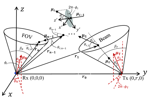
Figure 1: Geometry setting for the multiple-scattering process of NLOS UV communications

We first introduce the geometry setting for the multiple-scattering process of NLOS UV communications, shown in Fig. 1. The receiver (Rx) locates at the origin $(0,0,0)$ and the transmitter (Tx) locates at the $y$-axis with coordinates $(0,r,0)$. The direction cosines of Tx and Rx pointing directions are denoted by $\bm{\mu}_{T}$ and $\bm{\mu}_{R}$, respectively; The zenith angle and the azimuth angle of the Tx(Rx) are denoted by $\theta_{T(R)}$ and $\phi_{T(R)}$, respectively. The divergence angle of the Tx light beam is denoted by $\beta_{T}$ and the divergence angle of the Rx field-of-view (FOV) is denoted by $\beta_{R}$. We regard the initial photon emitting as the $zero$-order scattering and denote the propagating distance, scattering zenith angle and scattering azimuth angle of $i$-order scattering by $d_{i}$, $\theta_{i}$ and $\phi_{i}$, respectively. The position of the $i$th scatter is denoted by $\bm{r}_{i}$. The direction cosine of $i$-order scattering is denoted by $\bm{\mu}_{i}$. The initial scattering zenith angle $\theta_{0}$ is the angle between $\bm{\mu}_{0}$ and $\bm{\mu}_{T}$. We consider an $n$-order scattering process and define $\bm{d}\triangleq[d_{0},d_{1},\cdots,d_{n-1}]^{\text{T}}$, $\bm{\theta}\triangleq[\theta_{0},\theta_{1},\cdots,\theta_{n-1}]^{\text{T}}$, and $\bm{\phi}\triangleq[\phi_{0},\phi_{1},\cdots,\phi_{n-1}]^{\text{T}}$.

III-A Receiving Power Ignoring Turbulent Fluctuation

A photon propagating path of an $n$-order scattering is full characterized by the parameters $\{\bm{d},\bm{\theta},\bm{\phi}\}$. After scattered by the last scatter, the photon can be detected if and only if the position of the $n$th scatter locates in the FOV of the receiver. We denote the set of parameters satisfying this geometrical constrain by $\mathcal{F}\triangleq\{\bm{d},\bm{\theta},\bm{\phi}|\bm{r}_{n}\text{ in FOV}\}=\{\bm{d},\bm{\theta},\bm{\phi}|\bm{r}_{n}\cdot\bm{\mu}_{R}\geq d_{n}\cos(\beta_{R}/2)\}$. Then the conditional receiving probability of an $n$-order scattering process for a given propagating path $\{\bm{d},\bm{\theta},\bm{\phi}\}$ can be approximated as [17]

$$P_{n}(\bm{d},\bm{\theta},\bm{\phi}) =I_{n}(\bm{d},\bm{\theta},\bm{\phi})\left(\frac{k_{s}^{tot}}{k_{e}^{tot}}\right)^{n}\exp({-k_{e}^{tot}d_{n}})\cos\phi_{r}\min\left(1,p^{tot}(\theta_{r,n})\Omega_{r}\right),$$ (15)

where $d_{n}\triangleq\|\bm{r}_{n}\|$ and $\theta_{r,n}$ is the angle between $\bm{\mu}_{n-1}$ and $-\bm{r}_{n}$; $\phi_{r}$ is the angle between $\bm{\mu}_{R}$ and $\bm{r}_{n}$; $\Omega_{r}$ is the solid angle formed by $\bm{r}_{n}$ and the receiving area $A_{r}$; and we have $\Omega_{r}\approx 2\pi(1-d_{n}/\sqrt{d_{n}^{2}+r_{A}^{2}})$, where $r_{A}=\sqrt{A_{r}/\pi}$ is the radius of the receiving area; $I_{n}(\bm{d},\bm{\theta},\bm{\phi})$ is an indicator function; and we have $I_{n}(\bm{d},\bm{\theta},\bm{\phi})=1$ and $I_{n}(\bm{d},\bm{\theta},\bm{\phi})=0$ when the $n$th scatter locates within and without the FOV, respectively. Then the conditional receiving probability can be rewritten as

$$P_{n}(\bm{d},\bm{\theta},\bm{\phi})=\begin{cases}P_{d,n}(\bm{d},\bm{\theta},\bm{\phi}),\quad\{\bm{d},\bm{\theta},\bm{\phi}\}\in\mathcal{F},\\ 0,\quad\{\bm{d},\bm{\theta},\bm{\phi}\}\notin\mathcal{F},\end{cases}$$ (16)

where $P_{d,n}(\bm{d},\bm{\theta},\bm{\phi})\triangleq\left(\frac{k_{s}^{tot}}{k_{e}^{tot}}\right)^{n}\exp({-k_{e}^{tot}d_{n}})\cos\phi_{r}\min\left(1,\right.$ $\left.p^{tot}(\theta_{r,n})\Omega_{r}\right)$.

Then the receiving probability can be obtained by averaging $\{\bm{d},\bm{\theta},\bm{\phi}\}$ out, i.e.,

$$P_{n} =\int_{\bm{d}}\int_{\bm{\theta}}\int_{\bm{\phi}}P_{n}(\bm{d},\bm{\theta},\bm{\phi})f_{D,\Theta,\Phi}(\bm{d},\bm{\theta},\bm{\phi})\mathrm{d}\bm{d}\mathrm{d}\bm{\theta}\mathrm{d}\bm{\phi},$$ (17)

where $f_{D,\Theta,\Phi}(\bm{d},\bm{\theta},\bm{\phi})=\prod_{i=0}^{n-1}f_{D}(d_{i})f_{\Theta}(\theta_{i})f_{\Phi}(\phi_{i})$ is the joint PDF of $\{\bm{d},\bm{\theta},\bm{\phi}\}$. We have used the fact that $\bm{d}$, $\bm{\theta}$, and $\bm{\phi}$ are independent from each other. For the propagating distance $d_{i}$ with $i\in\{0,1,\cdots,n-1\}$, we have $f_{D}(d_{i})=k_{e}^{tot}e^{-k_{e}^{tot}d_{i}}$ with $0\leq d_{i}\leq\infty$ [17]. For the scattering angle $\theta_{i}$ with $i=0$, we have $f_{\Theta}(\theta_{0})=\frac{\sin\theta_{0}}{1-\cos({\beta_{T}}/{2})}$ with $0\leq\theta_{0}\leq{\beta_{T}}/{2}$ when a uniform light source is assumed [17]; and for the scattering angle $\theta_{i}$ with $i\in\{1,2,\cdots,n-1\}$, we have $f_{\Theta}(\theta_{i})=2\pi p^{tot}(\theta_{i})\sin\theta_{i}$ with $0\leq\theta_{i}\leq\pi$ [17]. For the scattering azimuth angle $\phi_{i}$ with $i\in\{0,1,\cdots,n-1\}$, we have $f_{\Phi}(\phi_{i})=\frac{1}{2\pi}$ with $0\leq\phi_{i}\leq 2\pi$ [17].

Without loss of generality, we assume that a unit light power is transmitted from the light source. Then the average receiving power equals the receiving probability $P_{n}$.

III-B Receiving Power Considering Turbulent Fluctuation

When the turbulent fluctuation effect is considered, a turbulent fading coefficient is introduced to each photon propagating distance. We denote the turbulent fading coefficient for the $i$th propagating distance $d_{i}$ by $\eta_{i}$. Then a photon propagating path $\{\bm{d},\bm{\theta},\bm{\phi}\}$ forms $(n+1)$ propagating distances $\{d_{0},d_{1},\cdots,d_{n}\}$, which corresponds to $(n+1)$ turbulent fading coefficients $\{\eta_{0},\eta_{1},\cdots,\eta_{n}\}$.

The conditional receiving probability without turbulent fluctuation for a given propagating path $\{\bm{d},\bm{\theta},\bm{\phi}\}$ is $P_{n}(\bm{d},\bm{\theta},\bm{\phi})$ given in (15). Then the conditional receiving probability under turbulent fluctuation effect for a given set of turbulent fading coefficients $\bm{\eta}\triangleq[\eta_{0},\eta_{1},\cdots,\eta_{n}]^{\text{T}}$ and a propagating path $\{\bm{d},\bm{\theta},\bm{\phi}\}$ can be expressed as

$$P_{tur,n}(\bm{\eta},\bm{d},\bm{\theta},\bm{\phi})=\prod_{i=0}^{n}\eta_{i}P_{n}(\bm{d},\bm{\theta},\bm{\phi}).$$ (18)

Then the receiving probability under turbulent fluctuation for a given propagating path $\{\bm{d},\bm{\theta},\bm{\phi}\}$ can be obtained by averaging $\bm{\eta}$ out, i.e.,

$$P_{tur,n}(\bm{d},\bm{\theta},\bm{\phi}) =\int_{\bm{\eta}}P_{tur,n}(\bm{\eta},\bm{d},\bm{\theta},\bm{\phi})f_{H|D,\Theta,\Phi}(\bm{\eta}|\bm{d},\bm{\theta},\bm{\phi})\mathrm{d}\bm{\eta},$$ (19)

where $f_{H|D,\Theta,\Phi}(\bm{\eta}|\bm{d},\bm{\theta},\bm{\phi})$ is the joint PDF of $\{\eta_{0},\eta_{1},\cdots,\eta_{n}\}$ conditioned on a given propagating path $\{\bm{d},\bm{\theta},\bm{\phi}\}$. For a given propagating path, $\eta_{0},\eta_{1},\cdots,\eta_{n}$ are assumed as independent variables. Then we have

$$f_{H|D,\Theta,\Phi}(\bm{\eta}|\bm{d},\bm{\theta},\bm{\phi})=\prod_{i=0}^{n}f_{H}(\eta_{i};d_{i}),$$ (20)

where $f_{H}(\eta;d)=f_{H,LN}(\eta;d)$ is given in (11) for LN distribution and $f_{H}(\eta;d)=f_{H,GG}(\eta;d)$ is given in (13) for GG distribution.

By substituting (18) and (20) into (19), we can obtain

$$P_{tur,n}(\bm{d},\bm{\theta},\bm{\phi}) =P_{n}(\bm{d},\bm{\theta},\bm{\phi})\prod_{i=0}^{n}\left[\int_{\eta_{i}}\eta_{i}f_{H}(\eta_{i};d_{i})\mathrm{d}\eta_{i}\right]=P_{n}(\bm{d},\bm{\theta},\bm{\phi}),$$ (21)

where we have used the property that $\int_{\eta_{i}}\eta_{i}f_{H}(\eta_{i};d_{i})\mathrm{d}\eta_{i}=1$ for $i=0,1,\cdots,n$.

Then the receiving probability considering the turbulent fluctuation effect can be obtained by averaging $\{\bm{d},\bm{\theta},\bm{\phi}\}$ out, i.e.,

$$P_{tur,n} =\int_{\bm{d}}\int_{\bm{\theta}}\int_{\bm{\phi}}P_{n}(\bm{d},\bm{\theta},\bm{\phi})f_{D,\Theta,\Phi}(\bm{d},\bm{\theta},\bm{\phi})\mathrm{d}\bm{d}\mathrm{d}\bm{\theta}\mathrm{d}\bm{\phi}=P_{n}.$$ (22)

From (22), we can see that $P_{tur,n}=P_{n}$, which indicates that the average receiving power considering the turbulent fluctuation equals the average receiving power ignoring the turbulent fluctuation. Therefore, in practical implementations, we can estimate the average receiving power by solving the integration in (17).

IV Estimating Turbulent Channels Using MCI Approach

IV-A Estimating the Average Receiving Power

The integration in (17) can be estimated by using the Monte-Carlo methods. In this paper, we use the MCI approach to estimate the average receiving power in (17). Compared with another widely used Monte-Carlo simulation (MCS) approach [13, 14], the MCI approach [15, 16, 17, 18, 19] enjoys a more flexible sampling function, resulting in a higher computational efficiency. Specifically, we can rewrite (17) as

$$P_{n}=\int_{\bm{d}}\int_{\bm{\theta}}\int_{\bm{\phi}}g_{n}(\bm{d},\bm{\theta},\bm{\phi})\mathrm{d}\bm{d}\mathrm{d}\bm{\theta}\mathrm{d}\bm{\phi},$$ (23)

where $g_{n}(\bm{d},\bm{\theta},\bm{\phi})$ is defined as $g_{n}(\bm{d},\bm{\theta},\bm{\phi})\triangleq P_{n}(\bm{d},\bm{\theta},\bm{\phi})f_{D,\Theta,\Phi}(\bm{d},\bm{\theta},\bm{\phi})$, and where $P_{n}(\bm{d},\bm{\theta},\bm{\phi})$ is given in (16). Now we can choose a sampling PDF $f_{n}(\bm{d},\bm{\theta},\bm{\phi})$ and further rewrite the receiving power $P_{n}$ in (23) as

$$P_{n} =\int_{\bm{d}}\int_{\bm{\theta}}\int_{\bm{\phi}}O_{n}(\bm{d},\bm{\theta},\bm{\phi})f_{n}(\bm{d},\bm{\theta},\bm{\phi})\mathrm{d}\bm{d}\mathrm{d}\bm{\theta}\mathrm{d}\bm{\phi}=\text{E}[O_{n}(\bm{d},\bm{\theta},\bm{\phi})],$$ (24)

where $O_{n}(\bm{d},\bm{\theta},\bm{\phi})\triangleq g_{n}(\bm{d},\bm{\theta},\bm{\phi})/f_{tur,n}(\bm{d},\bm{\theta},\bm{\phi})$ is called the objective function of MCI approach; and $\text{E}[x]$ denotes the expectation of $x$. Therefore, we have expressed the receiving power $P_{n}$ as the expectation of the objective function $O_{n}(\bm{d},\bm{\theta},\bm{\phi})$ when the joint PDF of $\{\bm{d},\bm{\theta},\bm{\phi}\}$ is the sampling PDF $f_{n}(\bm{d},\bm{\theta},\bm{\phi})$.

Different sampling PDF $f_{n}(\bm{d},\bm{\theta},\bm{\phi})$ can result in different computational efficiency of MCI approach [15, 16, 17]. Here we adopt the so-called important sampling method [15], which enjoys the same convergent speed as the MCS approach. The sampling PDF of the important sampling is given by

$$f_{n}(\bm{d},\bm{\theta},\bm{\phi})=f_{D,\Theta,\Phi}(\bm{d},\bm{\theta},\bm{\phi})=\prod_{i=0}^{n-1}f_{D}(d_{i})f_{\Theta}(\theta_{i})f_{\Phi}(\phi_{i}).$$ (25)

According to the sampling PDF $f_{n}(\bm{d},\bm{\theta},\bm{\phi})$ in (25), we can obtain the sampling functions for generating the propagating distance, the scattering angle, and the scattering azimuth angle as

$$d_{i}=-\frac{\ln(1-\text{rand}(1))}{k_{e}^{tot}},\quad i=0,1,\cdots,n-1,$$ (26)

$$\theta_{i}=\begin{cases}\arccos\left(1-\text{rand}(1)\times\left(1-\cos(\beta_{T}/2)\right)\right),\quad i=0,\\ F_{\Theta}^{-1}(\text{rand}(1)),\quad i=1,2,\cdots,n-1,\end{cases}$$ (27)

$$\phi_{i}=2\pi\times\text{rand}(1),\quad i=0,1,\cdots,n-1,$$ (28)

where $\text{rand}(1)$ is a random number between 0 and 1; $F_{\Theta}^{-1}(\theta_{s})$ is the inverse function of the cumulative distribution function of the scattering angle, i.e., $F_{\Theta}(\theta_{s})=\int_{0}^{\theta_{s}}f_{\Theta}(\theta)\mathrm{d}\theta$, which can be obtained as

$$F_{\Theta}(\theta_{s}) =C_{1}\cos\theta_{s}+C_{2}\cos^{3}\theta_{s}+C_{3}+C_{4}(C_{5}-C_{6}\cos\theta_{s})^{-1/2}+\frac{C_{7}(1-\cos\theta_{s})}{2+C_{8}(1-\cos\theta_{s})},$$ (29)

where $C_{1}=-\frac{3(1+3\gamma)}{8(1+2\gamma)}\frac{k_{s}^{ray}}{k_{s}^{tot}}+\frac{f(1-g^{2})}{4(1+g^{2})^{3/2}}\frac{k_{s}^{mie}}{k_{s}^{tot}}$, $C_{2}=-\frac{1-\gamma}{8(1+2\gamma)}\frac{k_{s}^{ray}}{k_{s}^{tot}}-\frac{f(1-g^{2})}{4(1+g^{2})^{3/2}}\frac{k_{s}^{mie}}{k_{s}^{tot}}$, $C_{3}=\frac{1}{2}\frac{k_{s}^{ray}}{k_{s}^{tot}}+\frac{1+g}{2g}\frac{k_{s}^{mie}}{k_{s}^{tot}}$, $C_{4}=-\frac{1-g^{2}}{2g}\frac{k_{s}^{mie}}{k_{s}^{tot}}$, $C_{5}=1+g^{2}$, $C_{6}=2g$, $C_{7}=(1+4k^{2}d_{0}^{2})\frac{k_{s}^{tur}}{k_{s}^{tot}}$, and $C_{8}=4k^{2}d_{0}^{2}$. For $i=1,2,\cdots,n-1$, the scattering angle $\theta_{i}$ can be solved by using numerical methods, e.g., Newton’s bisection search.

Then the corresponding objective function becomes

$$O_{n}(\bm{d},\bm{\theta},\bm{\phi}) =P_{n}(\bm{d},\bm{\theta},\bm{\phi})=\begin{cases}P_{d,n},\quad\{\bm{d},\bm{\theta},\bm{\phi}\}\in\mathcal{F},\\ 0,\quad\{\bm{d},\bm{\theta},\bm{\phi}\}\notin\mathcal{F}.\end{cases}$$ (30)

According to the law of large numbers, we can estimate the expectation $P_{n}$ using the average of sampling values for the objective function. Specifically, we can first randomly generate $M$ sampling points $\{\bm{s}_{n}^{1},\bm{s}_{n}^{2},\cdots,\bm{s}_{n}^{M}\}$ according to the sampling PDF given in (25), where we have

$$\bm{s}_{n}^{m}\triangleq[d_{0}^{m},\theta_{0}^{m},\phi_{0}^{m},\cdots,d_{n-1}^{m},\theta_{n-1}^{m},\phi_{n-1}^{m}]^{\text{T}}.$$ (31)

Then we can approximate the receiving power when $M$ is large as

$$P_{n}=\frac{1}{M}\sum_{m=1}^{M}O_{n}(\bm{s}_{n}^{m}).$$ (32)

The total receiving power over $N$ scattering orders can be obtained as

$$P_{tot}=\sum_{n=1}^{N}P_{n}=\frac{1}{M}\sum_{m=1}^{M}\sum_{n=1}^{N}O_{n}(\bm{s}_{n}^{m}).$$ (33)

IV-B Estimating the Channel Impulse Response

For each sampling point $\bm{s}_{n}^{m}$, we can calculating the corresponding receiving time as

$$t_{n}^{m}=\frac{\sum_{i=0}^{n}d_{i}^{m}}{c},$$ (34)

where $c$ is the light speed in the atmosphere. Then according to the result in [17], we can obtain the CIR of the multiple-scattering of UV communications in the following steps:

• Step 1: Classify the objective function value $O_{n}(\bm{s}_{n}^{m})$ into $L$ different time slots $\{(0,\Delta t)$, $(\Delta t,2\Delta t),\cdots,((L-1)\Delta t,L\Delta t)\}$ according to its receiving time $t_{n}^{m}$, where $\Delta t$ is a pre-chosen time interval;

• Step 2: Add up objective function values in each time slot and divide it by the number of sampling points $M$. Then we obtain the receiving probability sequences $[{P}_{n}(\Delta t),{P}_{n}(2\Delta t)$, $\cdots,{P}_{n}(L\Delta t)]^{\text{T}}$;

• Step 3: The CIR is obtained by normalizing the sequences $[{P}_{n}(\Delta t),{P}_{n}(2\Delta t),\!\cdots,\!{P}_{n}(L\Delta t)]^{\text{T}}$ using the receiving time interval $\Delta t$ and the receiving area $A_{r}$. Therefore, the value of CIR in a unit of irradiance at $t=l\Delta t$ is given by

  $$h_{n}(l\Delta t)=\frac{P_{n}(l\Delta t)}{\Delta_{t}A_{r}},\quad l=1,2\cdots,L.$$ (35)

Then the total CIR at $t=l\Delta t$ over $N$ scattering orders can be obtained as

$$h_{tot}(l\Delta t)=\sum_{n=1}^{N}\frac{P_{n}(l\Delta t)}{\Delta_{T}A_{r}},\quad l=1,2\cdots,L.$$ (36)

IV-C Estimating the Turbulent Fluctuation

It is challenging to estimate the turbulent fluctuation of the receiving power by using Monte-Carlo based methods. This is because the Monte-Carlo process itself will introduce a fluctuation effect on the calculated average receiving power [17]. In existing literature [52], the turbulent fluctuation was estimated by simply calculating the variance of the average receiving power $P_{tur,n}$, i.e, $\text{Var}[P_{tur,n}]$, obtained from the Monte-Carlo models. However, because $P_{tur,n}=P_{n}$, using the expression in (32), we can obtain

$$\text{Var}[P_{tur,n}]=\frac{1}{M^{2}}\sum_{m=1}^{M}\text{Var}[O_{n}(\bm{s}_{n}^{m})]=\frac{1}{M}\text{Var}[O_{n}(\bm{d},\bm{\theta},\bm{\phi})],$$ (37)

where we have used the fact that all sampling points $\{\bm{s}_{n}^{1},\bm{s}_{n}^{2},\cdots,\bm{s}_{n}^{M}\}$ are independent from each other and $\text{Var}[O_{n}(\bm{s}_{n}^{1})]=\text{Var}[O_{n}(\bm{s}_{n}^{2})]\cdots=\text{Var}[O_{n}(\bm{s}_{n}^{M})]=\text{Var}[O_{n}(\bm{d},\bm{\theta},\bm{\phi})]$ is the variance of the objective function. We can see that the variance $\text{Var}[P_{tur,n}]$ depends on both $\text{Var}[O_{n}(\bm{d},\bm{\theta},\bm{\phi})]$ and $M$. Besides, we have $\text{Var}[P_{tur,n}]\to 0$ when the number of sampling points $M\to\infty$, which means the calculated variance can be arbitrarily small as long as $M$ is large enough. Whereas, larger sampling points $M$ in the Monte-Carlo process only reduce the fluctuation caused by randomness, leading to more stable and precise results. Therefore, any attempt to calculate the turbulent fluctuation by estimating $\text{Var}[P_{tur,n}]$ will fail due to the fact that $\text{Var}[P_{tur,n}]$ depends on $M$. Here we present an improved estimating method for the turbulent fluctuation, which is independent of $M$.

By substituting (16) into (18), we can obtain

$$P_{tur,n}(\bm{\eta},\bm{d},\bm{\theta},\bm{\phi})=\begin{cases}\prod_{i=0}^{n}\eta_{i}P_{d,n}(\bm{d},\bm{\theta},\bm{\phi}),\quad\{\bm{d},\bm{\theta},\bm{\phi}\}\in\mathcal{F},\\ 0,\quad\{\bm{d},\bm{\theta},\bm{\phi}\}\notin\mathcal{F},\end{cases}$$ (38)

which can be regarded as a function of random variables $\bm{\eta}$, $\bm{d}$, $\bm{\theta}$, and $\bm{\phi}$. Therefore, the randomness of the receiving power comes from both the turbulent fading $\bm{\eta}$ and the propagating path $\{\bm{d},\bm{\theta},\bm{\phi}\}$. To characterize the turbulent fluctuation effect only, we can average $\{\bm{d},\bm{\theta},\bm{\phi}\}$ out and obtain the instantaneous receiving power conditioned on turbulent fading coefficients as

$$P_{tur,n}(\bm{\eta}) =\!\prod_{i=0}^{n}\eta_{i}\!\!\int_{\bm{d}}\int_{\bm{\theta}}\int_{\bm{\phi}}\!P_{n}(\bm{d},\bm{\theta},\bm{\phi})f_{D,\Theta,\Phi}(\bm{d},\bm{\theta},\bm{\phi})\mathrm{d}\bm{d}\mathrm{d}\bm{\theta}\mathrm{d}\bm{\phi}=\!{\prod_{i=0}^{n}\eta_{i}}P_{n}.$$ (39)

Then we can define an equivalent turbulent fading coefficient $\eta_{eq,n}\triangleq P_{tur,n}(\bm{\eta})/P_{n}$ on the average receiving power $P_{n}$ such that the instantaneous receiving power $P_{tur,n}(\bm{\eta})=\eta_{eq,n}P_{n}$. Obviously, we have

$$\eta_{eq,n}=\prod_{i=0}^{n}\eta_{i}.$$ (40)

One can easily verify that $\text{E}[\eta_{eq,n}]=1$. Then the turbulent fluctuation for the $n$th scattering order can be fully characterized by the turbulent variance

$$\sigma_{tur,n}^{2} \triangleq\text{Var}[\eta_{eq,n}]=\int_{\bm{\eta}}(\eta_{eq,n}-1)^{2}f_{H}(\bm{\eta})\mathrm{d}\bm{\eta},$$ (41)

where $f_{H}(\bm{\eta})$ is the joint PDF of $\{\eta_{0},\eta_{1},\cdots,\eta_{n}\}$. From (38) we can see that those propagating paths with $\{\bm{d},\bm{\theta},\bm{\phi}\}\notin\mathcal{F}$ contribute zero to the turbulent fluctuation effect. Therefore, we should restrict the variance on the set $\mathcal{F}$. Then the joint PDF $f_{H}(\bm{\eta})$ can be obtained by averaging $\{\bm{d},\bm{\theta},\bm{\phi}\}$ out of the conditional PDF $f_{H|D,\Theta,\Phi}(\bm{\eta}|\bm{d},\bm{\theta},\bm{\phi})$ in (20) on the set $\mathcal{F}$, i.e.,

$$f_{H}(\bm{\eta}) \!=\!\int_{\mathcal{F}}f_{D,\Theta,\Phi}(\bm{d},\bm{\theta},\bm{\phi}|\{\bm{d},\bm{\theta},\bm{\phi}\}\in\mathcal{F})f_{H|D,\Theta,\Phi}(\bm{\eta}|\bm{d},\bm{\theta},\bm{\phi})\mathrm{d}\bm{d}\mathrm{d}\bm{\theta}\mathrm{d}\bm{\phi},$$ (42)

where $f_{D,\Theta,\Phi}(\bm{d},\bm{\theta},\bm{\phi}|\{\bm{d},\bm{\theta},\bm{\phi}\}\in\mathcal{F})$ is the joint PDF of $\{\bm{d},\bm{\theta},\bm{\phi}\}$ on the set $\mathcal{F}$; and we have

$$f_{D,\Theta,\Phi}(\bm{d},\bm{\theta},\bm{\phi}|\{\bm{d},\bm{\theta},\bm{\phi}\}\in\mathcal{F}) =\frac{f_{D,\Theta,\Phi}(\bm{d},\bm{\theta},\bm{\phi})}{\text{Pr}[\{\bm{d},\bm{\theta},\bm{\phi}\}\in\mathcal{F}]},$$ (43)

where $\text{Pr}[\{\bm{d},\bm{\theta},\bm{\phi}\}\in\mathcal{F}]$ is the probability of $\{\bm{d},\bm{\theta},\bm{\phi}\}\in\mathcal{F}$ given by

$$\text{Pr}[\{\bm{d},\bm{\theta},\bm{\phi}\}\in\mathcal{F}]=\int_{\mathcal{F}}f_{D,\Theta,\Phi}(\bm{d},\bm{\theta},\bm{\phi})\mathrm{d}\bm{d}\mathrm{d}\bm{\theta}\mathrm{d}\bm{\phi}.$$ (44)

By substituting (20), (43), and (44) into (42), we can obtain

$$f_{H}(\bm{\eta}) =\frac{\int_{\mathcal{F}}\prod_{i=0}^{n}f_{H}(\eta_{i};d_{i})f_{D,\Theta,\Phi}(\bm{d},\bm{\theta},\bm{\phi})\mathrm{d}\bm{d}\mathrm{d}\bm{\theta}\mathrm{d}\bm{\phi}}{\int_{\mathcal{F}}f_{D,\Theta,\Phi}(\bm{d},\bm{\theta},\bm{\phi})\mathrm{d}\bm{d}\mathrm{d}\bm{\theta}\mathrm{d}\bm{\phi}}$$ (45)

$$=\frac{\int_{\bm{d}}\int_{\bm{\theta}}\int_{\bm{\phi}}\prod_{i=0}^{n}f_{H}(\eta_{i};d_{i})I_{n}f_{D,\Theta,\Phi}(\bm{d},\bm{\theta},\bm{\phi})\mathrm{d}\bm{d}\mathrm{d}\bm{\theta}\mathrm{d}\bm{\phi}}{\int_{\bm{d}}\int_{\bm{\theta}}\int_{\bm{\phi}}I_{n}f_{D,\Theta,\Phi}(\bm{d},\bm{\theta},\bm{\phi})\mathrm{d}\bm{d}\mathrm{d}\bm{\theta}\mathrm{d}\bm{\phi}}.$$

Then by substituting (40) and (45) into (41), we can obtain the turbulent variance as

$$\sigma_{tur,n}^{2} \!=\!\frac{\int_{\bm{d}}\int_{\bm{\theta}}\int_{\bm{\phi}}(\prod_{i=0}^{n}M_{2}(d_{i})-1)I_{n}f_{D,\Theta,\Phi}(\bm{d},\bm{\theta},\bm{\phi})\mathrm{d}\bm{d}\mathrm{d}\bm{\theta}\mathrm{d}\bm{\phi}}{\int_{\bm{d}}\int_{\bm{\theta}}\int_{\bm{\phi}}I_{n}(\bm{d},\bm{\theta},\bm{\phi})f_{D,\Theta,\Phi}(\bm{d},\bm{\theta},\bm{\phi})\mathrm{d}\bm{d}\mathrm{d}\bm{\theta}\mathrm{d}\bm{\phi}},$$ (46)

where $M_{2}(d_{i})$ is the second-order moment of the turbulent fading coefficient $\eta_{i}(d_{i})$. For LN distribution, we have $M_{2}(d_{i})=\exp(\sigma_{r}^{2}(d_{i}))$; and for GG distribution, we have $M_{2}(d_{i})=(1+1/\alpha(d_{i}))(1+1/\beta(d_{i}))$.

Similar to the estimation of the average receiving power $P_{n}$, we can also use the MCI approach to estimate both the nominator and the denominator of $\sigma_{tur,n}^{2}$ in (46) using the same sampling PDF given in (25). Then using the same sampling points $\{\bm{s}_{n}^{1},\bm{s}_{n}^{2},\cdots,\bm{s}_{n}^{M}\}$, we can estimate the turbulent variance $\sigma_{tur,n}^{2}$ as

$$\sigma_{tur,n}^{2} =\frac{\frac{1}{M}\sum_{m=1}^{M}\left[\prod_{i=0}^{n}M_{2}(d_{i}^{m})-1\right]I_{n}(\bm{s}_{n}^{m})}{\frac{1}{M}\sum_{m=0}^{M}I_{n}(\bm{s}_{n}^{m})}=\frac{1}{Count}\sum_{m=1}^{M}\left[\prod_{i=0}^{n}M_{2}(d_{i}^{m})-1\right]I_{n}(\bm{s}_{n}^{m}),$$ (47)

where $Count\triangleq\sum_{m=0}^{M}I_{n}(\bm{s}_{n}^{m})$ is the number of sampling points satisfying $\{\bm{d},\bm{\theta},\bm{\phi}\}\in\mathcal{F}$.

Similar to the $n$th scattering order, the total turbulent fluctuation effect on the total receiving power of $N$ scattering orders can be characterized by defining an equivalent turbulent fading coefficient $\eta_{eq}\triangleq\sum_{n=1}^{N}P_{tur,n}(\bm{\eta})/\sum_{n=1}^{N}P_{n}$. Using the relations $P_{tur,n}(\bm{\eta})=\eta_{eq,n}P_{n}$ and $P_{tot}=\sum_{n=1}^{N}P_{n}$, we can obtain

$$\eta_{eq} =\sum_{n=1}^{N}\frac{P_{n}}{P_{tot}}\eta_{eq,n}.$$ (48)

Then the total turbulent variance $\sigma_{tur}^{2}$ for $N$ scattering orders can be obtained as

$$\sigma_{tur}^{2} \triangleq\text{Var}[\eta_{eq}]=\sum_{n=1}^{N}\left(\frac{P_{n}}{P_{tot}}\right)^{2}\sigma_{tur,n}^{2},$$ (49)

where $P_{n}$, $P_{tot}$, and $\sigma_{tur,n}^{2}$ are given by (32), (33), and (47), respectively.

IV-D Estimating the Distribution of Turbulent Fading Coefficient

It is challenging to derive the distribution of the turbulent fading coefficient for a general turbulent fading model. However, when the turbulence is weak and an LN fading is considered, then we can further derive the distributions of the equivalent turbulent fading coefficients $\eta_{eq,n}$ and $\eta_{eq}$. For a given propagating path $\{\bm{d},\bm{\theta},\bm{\phi}\}$, the equivalent turbulent fading coefficient $\eta_{eq,n}$ can be obtained from (40) as

$$\eta_{eq,n}(\bm{d},\bm{\theta},\bm{\phi})=\prod_{i=0}^{n}\eta_{i}(\bm{d},\bm{\theta},\bm{\phi}).$$ (50)

The logarithm of $\eta_{eq,n}(\bm{d},\bm{\theta},\bm{\phi})$ is

$$\ln\eta_{eq,n}(\bm{d},\bm{\theta},\bm{\phi})=\sum_{i=0}^{n}\ln\eta_{i}(\bm{d},\bm{\theta},\bm{\phi}).$$ (51)

Because $\eta_{i}(\bm{d},\bm{\theta},\bm{\phi})$ satisfies an LN distribution with parameter $\sigma_{I}^{2}(d_{i})$ and $\{\eta_{0},\eta_{1},\cdots,\eta_{n}$ are independent variables, from (51) we can see that $\eta_{eq,n}(\bm{d},\bm{\theta},\bm{\phi})$ also satisfies an LN distribution with parameter $\sigma_{eq,n}^{2}(\bm{d},\bm{\theta},\bm{\phi})=\sum_{i=0}^{n}\sigma_{I}^{2}(d_{i})$. Therefore, the conditional PDF of $\eta_{eq,n}(\bm{d},\bm{\theta},\bm{\phi})$ is given by

$$f_{H,n}(\eta_{eq,n}|\bm{d},\bm{\theta},\bm{\phi}) =\frac{1}{\eta_{eq,n}\sqrt{2\pi\sigma_{eq,n}^{2}(\bm{d},\bm{\theta},\bm{\phi})}}\exp\left(\!{-\frac{(\ln\eta_{eq,n}+0.5\sigma_{eq,n}^{2}(\bm{d},\bm{\theta},\bm{\phi}))^{2}}{2\sigma_{eq,n}^{2}(\bm{d},\bm{\theta},\bm{\phi})}}\!\right).$$ (52)

Then the unconditional PDF for the equivalent turbulent fading coefficient $\eta_{eq,n}$ can be obtained by averaging $\{\bm{d},\bm{\theta},\bm{\phi}\}$ on $\mathcal{F}$ out, which is given by

$$f_{H,n}(\eta_{eq,n}) =\frac{\int_{\bm{d}}\int_{\bm{\theta}}\int_{\bm{\phi}}\frac{I_{n}(\bm{d},\bm{\theta},\bm{\phi})}{\eta_{eq,n}\sqrt{2\pi\sum_{i=0}^{n}\sigma_{I}^{2}(d_{i})}}\exp\left({-\frac{(\ln\eta_{eq,n}+0.5\sum_{i=0}^{n}\sigma_{I}^{2}(d_{i}))^{2}}{2\sum_{i=0}^{n}\sigma_{I}^{2}(d_{i})}}\right)f_{D,\Theta,\Phi}(\bm{d},\bm{\theta},\bm{\phi})\mathrm{d}\bm{d}\mathrm{d}\bm{\theta}\mathrm{d}\bm{\phi}}{\int_{\bm{d}}\int_{\bm{\theta}}\int_{\bm{\phi}}I_{n}(\bm{d},\bm{\theta},\bm{\phi})f_{D,\Theta,\Phi}(\bm{d},\bm{\theta},\bm{\phi})\mathrm{d}\bm{d}\mathrm{d}\bm{\theta}\mathrm{d}\bm{\phi}}.$$ (53)

Then we can also use the MCI approach to estimate $f_{H}(\eta_{eq,n})$ using the same sampling PDF given in (25). Using the same sampling points $\{\bm{s}_{n}^{1},\bm{s}_{n}^{2},\cdots,\bm{s}_{n}^{M}\}$, we can estimate the PDF of equivalent turbulent fading coefficient $f_{H}(\eta_{eq,n})$ as

$$f_{H,n}(\eta_{eq,n}) =\frac{1}{Count}\sum_{m=1}^{M}\frac{I_{n}(\bm{s}_{n}^{m})}{\eta_{eq,n}\sqrt{2\pi\sum_{i=0}^{n}\sigma_{I}^{2}(d_{i}^{m})}}\exp\left({-\frac{(\ln\eta_{eq,n}+0.5\sum_{i=0}^{n}\sigma_{I}^{2}(d_{i}^{m}))^{2}}{2\sum_{i=0}^{n}\sigma_{I}^{2}(d_{i}^{m})}}\right).$$ (54)

According to (48), the PDF of the total equivalent turbulent fading coefficient $\eta_{eq}$ for $N$ scattering orders can be obtained as the convolution of the PDFs of $\{\frac{P_{1}}{P_{tot}}\eta_{eq,1},\frac{P_{2}}{P_{tot}}\eta_{eq,2},\cdots,\frac{P_{N}}{P_{tot}}\eta_{eq,N}\}$, i.e.,

$$f_{H}(\eta_{eq}) =\frac{P_{tot}}{P_{1}}f_{H,1}\left(\frac{P_{tot}}{P_{1}}\eta_{eq}\right)*\frac{P_{tot}}{P_{2}}f_{H,2}\left(\frac{P_{tot}}{P_{2}}\eta_{eq}\right)*\cdots*\frac{P_{tot}}{P_{N}}f_{H,N}\left(\frac{P_{tot}}{P_{N}}\eta_{eq}\right),$$ (55)

where $*$ denotes the convolution operation and $f_{H,n}(x)$ is calculated by (54).

The pseudocode of the MCI approach is similar to the one we presented in [17]. The only difference is that we need to add the estimation of turbulent fluctuation and distribution in each MCI process according to the equations given in (47) and (54), respectively.

V Numerical Results and Discussions

In this section, we present some numerical results to verify our theoretical analysis and discuss some interesting findings. Unless otherwise specified, the simulation parameters we used in this section are listed in Table I. Without loss of generality, we set $C_{n}^{2}=10^{-17}$ $\text{m}^{-2/3}$, $C_{n}^{2}=10^{-15}$ $\text{m}^{-2/3}$, and $C_{n}^{2}=10^{-13}$ $\text{m}^{-2/3}$ for weak, moderate, and strong turbulent conditions, respectively.

TABLE I: Simulation Parameters

Parameters	Values
$r$	$500$ m
$[\theta_{T},\phi_{T}]$	$[45^{\circ},-90^{\circ}]$
$[\theta_{R},\phi_{R}]$	$[45^{\circ},90^{\circ}]$
$[\beta_{T},\beta_{R}]$	$[17^{\circ},30^{\circ}]$
$A_{r}$	$1.77\times 10^{-4}{\text{m}}^{2}$
$\lambda$	$2.6\times 10^{-7}$ m
$c$	$2.998\times 10^{8}$ $\text{m}/\text{s}$
$[k_{a}^{par},k_{s}^{ray},k_{s}^{mie}]$	$[0.802,0.266,0.284]$ ${\text{km}}^{-1}$
$[\gamma,g,f]$	$[0.017,0.72,0.5]$
$L_{0}$	$10^{2}$ m
$d_{0}$	$10^{-3}$ m
$C_{n}^{2}$	$10^{-15}$ $\text{m}^{-2/3}$
$\Delta t$	$0.02$ $\mu$s
$M$	$10^{6}$
$N$	$3$

V-A Results for Turbulence-Induced Scattering Effect

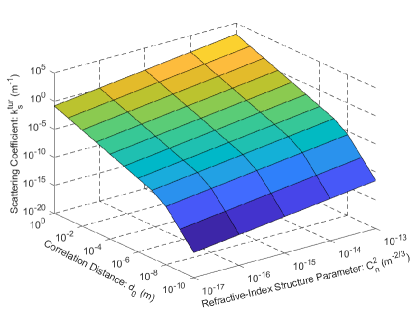
(a)

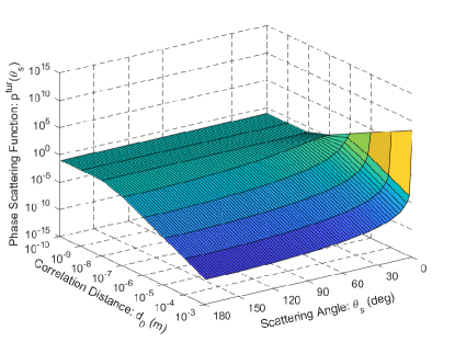
(b)

Figure 2: Turbulence-induced scattering effect: (a) scattering coefficient $k_{s}^{tur}$ under different $C_{n}^{2}$ and $d_{0}$; (b) phase scattering function $p^{tur}(\theta_{s})$ at different $\theta_{s}$ and $d_{0}$

We first explore the turbulence-induced scattering coefficient $k_{s}^{tur}$ and phase scattering function $p^{tur}(\theta_{s})$ under different turbulent parameters in Fig. 2. Fig. 2(a) presents the scattering coefficient $k_{s}^{tur}$ under different refractive-index structure parameter $C_{n}^{2}$ and correlation distance $d_{0}$. From Fig. 2(a) we can see that the scattering coefficient $k_{s}^{tur}$ increases as either the turbulence strength or the correlation distance increases. Besides, for a given refractive-index structure parameter $C_{n}^{2}$, the slop of the turbulent scattering coefficient $k_{s}^{tur}$ for $d_{0}\gg\lambda$ is much smaller than that for $d_{0}\ll\lambda$, where $\lambda=2.6\times 10^{-7}$ m. These observations verified our theoretical analysis on Eq. (6). Fig. 2(b) presents the phase scattering function $p^{tur}(\theta_{s})$ at different scattering angle $\theta_{s}$ and correlation distance $d_{0}$. Note that $L_{0}$ and $C_{n}^{2}$ have no impact on the phase scattering function. From Fig. 2(b), we can see that, when $d_{0}\gg\lambda$, the scattering intensity rapidly increases as the scattering angle decreases. This indicates that the incident photons will have a high probability of maintaining their original traveling direction after scattering. By contrast, when $d_{0}\ll\lambda$, we can see that the phase scattering function varies slowly at different scattering angles and will finally approximate an isotropic scattering. These observations verified our theoretical analysis on Eq. (7).

The impacts of turbulence-induced scattering effect on the receiving power of NLOS UV communications should be explored by considering both the scattering coefficient $k_{s}^{tur}$ and the phase scattering function $p^{tur}(\theta_{s})$. Combining the results in Figs. 2(a) and 2(b), we have the following observations:

• When $d_{0}\ll\lambda$, we have $k_{s}^{tur}\to 0$; in this case, though the phase scattering function approaches an isotropic scattering, the overall impact of the turbulence-induced scattering effect is negligible compared with the scattering effect due to particles; therefore, we can always ignore the turbulence-induced scattering effect when $d_{0}\ll\lambda$.

• When $d_{0}\gg\lambda$, the scattering is almost a complete forward scattering since almost all the scattering intensity concentrates at $\theta_{s}=0^{\circ}$; in this case, though there exists large scattering coefficient $k_{s}^{tur}\gg 1$, the overall turbulence-induced scattering can be equivalently regarded as a rectilinear propagation with negligible divergence angle, which means no evident impact on the final receiving power can be observed; therefore, we can also ignore the turbulence-induced scattering effect when $d_{0}\gg\lambda$.

• When $d_{0}\sim\lambda$, the phase scattering function is not a complete forward scattering; then we cannot ignore the turbulence-induced scattering effect if the scattering coefficient $k_{s}^{tur}$ is not negligible compared with $k_{s}^{par}$, which can happen under strong turbulent conditions; for example, when $d_{0}=10^{-7}$ m, $C_{n}^{2}=10^{-13}$ $\text{m}^{-2/3}$, and $L_{0}=10^{3}$ m, we have $k_{s}^{tur}=0.586$ $\text{km}^{-1}$, which is comparable with $k_{s}^{par}=0.550$ $\text{km}^{-1}$.

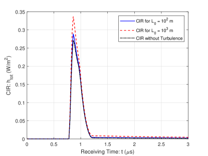
(a)

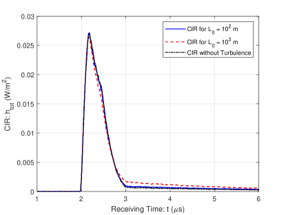
(b)

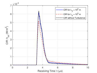
(c)

Figure 3: CIR results under different outer scale parameters $L_{0}$: (a) $r=200$ m; (b) $r=500$ m; (c) $r=800$ m

Let us explore the cases with $d_{0}\sim\lambda$. Fig. 3 presents the CIR results under different outer scale parameters $L_{0}$ in different communication distances $r\in\{200\ \text{m},500\ \text{m},800\ \text{m}\}$ with $d_{0}=10^{-7}$ m and $C_{n}^{2}=10^{-13}$ $\text{m}^{-2/3}$. Comparing Figs. 3(a), 3(b), and 3(c), we can see that when the communication distance is small, the turbulence-induced scattering can enhance the receiving power. However, as the communication distance increases, the enhancement due to the turbulence-induced scattering gradually decreases and finally the turbulence-induced scattering will introduce an extra attenuation on receiving power in large communication distance. Here we can explain this distance-dependent scaling effect on the receiving power. Since the single-scattering is the major scattering here, we roughly consider the single-scattering only. As we know, an increase in the scattering coefficient can not only increase the scattering strength but also increase the extinction strength and shorten the photon traveling distance. The expectation of the photon traveling distance can be estimated as $1/k_{e}^{tot}$ and here we have $1/k_{e}^{tot}=1/(k_{s}^{par}+k_{a}^{par})\approx 739.6$ m by ignoring the turbulence-induced scattering. Then when the communication distance is smaller than $739.6$ m, an increase in the scattering coefficient will shorten the expected traveling distance and thus increase the scattering strength in the common volume, and vice versa. Therefore, when $r=200$ m, the turbulence-induced scattering mainly acts as a scattering effect enhancer; whereas when $r=800$ m, the turbulence-induced scattering mainly acts as an extinction effect enhancer.

Though we have demonstrated that the turbulence-induced scattering effect can impact the final receiving power when $d_{0}\sim\lambda$, in practical implementations, we have $d_{0}\gg\lambda$ almost always holds. For example, the correlation distance $d_{0}$ is normally in between $l_{0}$ and $L_{0}$, where $l_{0}$ is the inner scale parameter representing the smallest turbulent eddy size; and $l_{0}$ is at the same order of magnitude with the Fresnel zone $R_{F}=(L/k)^{1/2}$, where $k$ is the light wave number and $L$ is the light propagating distance. For typical UV communication scenarios, we have $10^{0}\ \text{m}\leq L\leq 10^{4}\ \text{m}$ and $2.034\times 10^{-4}\ \text{m}\leq R_{F}\leq 2.034\times 10^{-2}\ \text{m}$, which results in $d_{0}\sim R_{F}\gg\lambda$. Therefore, we can conclude that the turbulence-induced scattering effect can always be ignored in typical UV communication scenarios.

V-B Results for Turbulent Fluctuation Effect

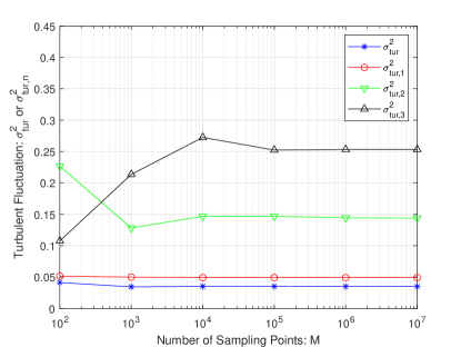
Figure 4: Turbulent fluctuations under different number of sampling points

Then we explore the turbulent fluctuation effects. Fig. 4 presents the estimated turbulent fluctuation under different number of sampling points $M$. As we can see from Fig. 4, the estimated turbulent fluctuation $\sigma^{2}_{tur}$ or $\sigma_{tur,n}^{2}$ will become stable as $M$ increases. Besides, we can also roughly estimate the turbulent variance by using the method proposed for the single-scattering link in [47]. Specifically, the turbulent variance can be approximated as $\sigma_{tur,1}^{2}\approx\exp(\sigma_{I}^{2}(r_{1})+\sigma_{I}^{2}(r_{2}))-1\approx 0.0493$, which is quite close to our result $\sigma_{tur,1}^{2}=0.0492$ in Fig. 4. This verified that our proposed estimation method for turbulent fluctuation can well estimate the turbulent variance.

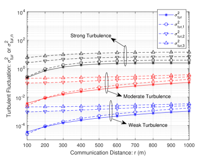
(a)

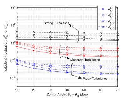
(b)

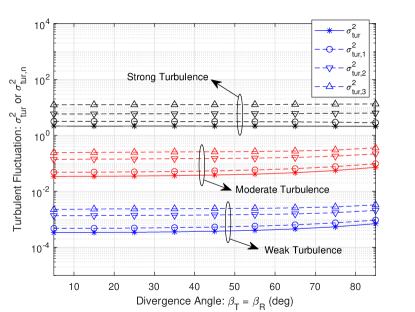
(c)

Figure 5: Turbulent fluctuations under various system geometries: (a) turbulent fluctuations under different communication distances; (b) turbulent fluctuations under different zenith angles; (c) turbulent fluctuations under different divergence angles

Then we present the turbulent fluctuations results under various system geometries in Fig. 5. From Figs. 5(a), 5(b) and 5(c), we can see that the turbulent variance increases as either the communication distance $r$, the elevation angle $\pi/2-\theta_{T}$, or the divergence angle $\beta_{T}$ increases, which is compatible with reported experimental results in [53, 54]. Besides, we can also observe that the turbulence variance will approach a stable value for strong turbulent conditions in Figs. 5(a), 5(b) and 5(c). This is because the channel will become a saturated turbulent channel under strong turbulence as either the communication distance $r$, the elevation angle $\pi/2-\theta_{T}$, or the divergence angle $\beta_{T}$ increases, which is compatible with the saturated turbulence case with $\sigma_{r}^{2}\to\infty$ at the end of Section II.

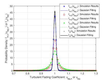
(a)

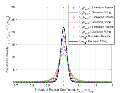
(b)

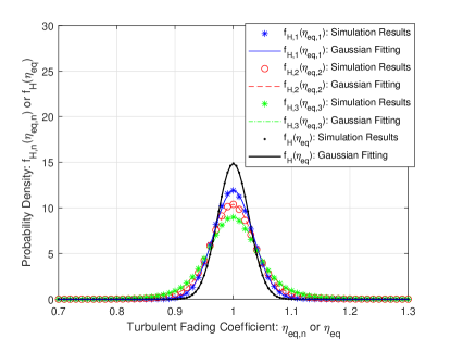
(c)

Figure 6: Distribution of turbulent fading coefficient under different distances: (a) $r=200$ m; (b) $r=500$ m; (c) $r=800$ m

At last, we present the estimated probability density for the turbulent fading coefficients under different communication distances $r\in\{200\ \text{m},500\ \text{m},800\ \text{m}\}$ with $C_{n}^{2}=10^{-17}$ $\text{m}^{-2/3}$ in Fig. 6. The simulation results of $f_{H,n}(\eta_{eq,n})$ for the $n$th order scattering are fitted with a weighted summation of $n$ Gaussian distributions, and the simulation results of $f_{H}(\eta_{eq})$ are fitted with a Gaussian distribution. From Fig. 6, we can see that the Gaussian fitting can well match the simulation results. Here we give an explanation on the single-scattering only. For a single-scattering, we can divide the common volume $V$ into many small volumes $\{v_{1},v_{2},\cdots,v_{L}\}$. Then according to the LN assumption in [47], the receiving power $P_{r}^{l}$ contributed from the $l$th volume $v_{l}$ follows a LN distribution. Then according to the central limit theorem, the total receiving power $P_{r}=\sum_{l=1}^{L}P_{r}^{l}$ will converge to a Gaussian distribution when $L$ is large.

VI Conclusion

Existing works on the modeling of multiple-scattering turbulent channels either ignored the turbulence-induced scattering effect or erroneously estimated the turbulent fluctuation effect on the NLOS UV communications. In this paper, we established a multiple-scattering turbulent channel model considering both the turbulence-induced scattering effect and the turbulent fluctuation effect. Numerical results demonstrated that, for typical UV communication scenarios, the turbulence-induced scattering effect can always be ignored; and the turbulent fluctuation will increase as either the communication distance, the elevation angle, or the divergence angle increases, which is compatible with existing experimental results. Besides, we also demonstrated that the distribution of the overall turbulent fading coefficient for the multiple-scattering process can be approximated as a Gaussian distribution.

References

- [1] R. J. Drost and B. M. Sadler, “Survey of ultraviolet non-line-of-sight communications,” Semicond. Sci. Technol., vol. 29, no. 8, p. 084006, June 2014.
- [2] R. Yuan and J. Ma, “Review of ultraviolet non-line-of-sight communication,” China Commun., vol. 13, no. 6, pp. 63–75, June 2016.
- [3] M. R. Luettgen, D. M. Reilly, and J. H. Shapiro, “Non-line-of-sight single-scatter propagation model,” J. Opt. Soc. Am. A, vol. 8, no. 12, pp. 1964–1972, Dec. 1991.
- [4] Z. Xu, H. Ding, B. M. Sadler, and G. Chen, “Analytical performance study of solar blind non-line-of-sight ultraviolet short-range communication links,” Opt. Lett., vol. 33, no. 16, pp. 1860–1862, Aug. 2008.
- [5] M. A. Elshimy and S. Hranilovic, “Non-line-of-sight single-scatter propagation model for noncoplanar geometries,” J. Opt. Soc. Am. A, vol. 28, no. 3, pp. 420–428, Mar. 2011.
- [6] Y. Zuo, H. Xiao, J. Wu, Y. Li, and J. Lin, “A single-scatter path loss model for non-line-of-sight ultraviolet channels,” Opt. Express, vol. 20, no. 9, pp. 10 359–10 369, Apr. 2012.
- [7] T. Wu, J. Ma, P. Su, R. Yuan, and J. Cheng, “Modeling of short-range ultraviolet communication channel based on spherical coordinate system,” IEEE Commun. Lett., vol. 23, no. 2, pp. 242–245, Feb. 2019.
- [8] T. Wu, J. Ma, R. Yuan, P. Su, and J. Cheng, “Single-scatter model for short-range ultraviolet communication in a narrow beam case,” IEEE Photonic. Tech. L, vol. 31, no. 3, pp. 265–268, Feb. 2019.
- [9] Z. Shen, J. Ma, T. Shan, and T. Wu, “Modeling of ultraviolet scattering propagation and its applicability analysis,” Optics letters, vol. 44, no. 20, pp. 4953–4956, Oct. 2019.
- [10] T. Cao, X. Gao, T. Wu, C. Pan, and J. Song, “Single-scatter path loss model of led-based non-line-of-sight ultraviolet communications,” Opt. Lett., vol. 46, no. 16, pp. 4013–4016, Aug. 2021.
- [11] T. Cao, J. Song, and C. Pan, “Simplified closed-form single-scatter path loss model of non-line-of-sight ultraviolet communications in noncoplanar geometry,” IEEE J. Quantum Electron., vol. 57, no. 2, pp. 1–9, Apr. 2021.
- [12] T. Cao, T. Wu, C. Pan, and J. Song, “Single-collision-induced path loss model of reflection-assisted non-line-of-sight ultraviolet communications,” Opt. Express, vol. 30, no. 9, pp. 15 227–15 237, Apr. 2022.
- [13] H. Ding, G. Chen, A. K. Majumdar, B. M. Sadler, and Z. Xu, “Modeling of non-line-of-sight ultraviolet scattering channels for communication,” IEEE J. Sel. Areas Commun., vol. 27, no. 9, pp. 1535–1544, Dec. 2009.
- [14] R. J. Drost, T. J. Moore, and B. M. Sadler, “UV communications channel modeling incorporating multiple scattering interactions,” J. Opt. Soc. Am. A, vol. 28, no. 4, pp. 686–695, Apr. 2011.
- [15] R. Yuan, J. Ma, P. Su, Y. Dong, and J. Cheng, “An importance sampling method for Monte-Carlo integration model for ultraviolet communication,” in 2019 International Conference on Advanced Communication Technologies and Networking (CommNet). IEEE, Apr. 2019, pp. 1–6.
- [16] H. Ding, Z. Xu, and B. M. Sadler, “A path loss model for non-line-of-sight ultraviolet multiple scattering channels,” EURASIP J. Wirel. Commun. Netw., vol. 2010, pp. 63:1–63:11, Apr. 2010.
- [17] R. Yuan, J. Ma, P. Su, Y. Dong, and J. Cheng, “Monte-Carlo integration models for multiple scattering based optical wireless communication,” IEEE Trans. Commun., vol. 68, no. 1, pp. 334–348, Nov. 2019.
- [18] T. Shan, J. Ma, T. Wu, Z. Shen, and P. Su, “Modeling of ultraviolet omni-directional multiple scattering channel based on monte carlo method,” Opt. Lett., vol. 45, no. 20, pp. 5724–5727, Oct. 2020.
- [19] Z. Shen, J. Ma, T. Shan, and P. Su, “Improved monte carlo integration models for ultraviolet communications,” in 2020 IEEE 20th International Conference on Communication Technology (ICCT). IEEE, 2020, pp. 168–172.
- [20] R. Yuan, J. Ma, P. Su, and Z. He, “An integral model of two-order and three-order scattering for non-line-of-sight ultraviolet communication in a narrow beam case,” IEEE Commun. Lett., vol. 20, no. 12, pp. 2366–2369, Sep. 2016.
- [21] M. A. El-Shimy and S. Hranilovic, “Binary-input non-line-of-sight solar-blind UV channels: Modeling, capacity and coding,” J. Opt. Commun., vol. 4, no. 12, pp. 1008–1017, Nov. 2012.
- [22] C. Gong and Z. Xu, “Channel estimation and signal detection for optical wireless scattering communication with inter-symbol interference,” IEEE Trans. Wirel. Commun., vol. 14, no. 10, pp. 5326–5337, Oct. 2015.
- [23] C. Gong, X. Zhang, Z. Xu, and L. Hanzo, “Optical wireless scattering channel estimation for photon-counting and photomultiplier tube receivers,” IEEE Trans. Commun., vol. 64, no. 11, pp. 4749–4763, Nov. 2016.
- [24] Z. Wei, W. Hu, D. Han, M. Zhang, B. Li, and C. Zhao, “Simultaneous channel estimation and signal detection in wireless ultraviolet communications combating inter-symbol-interference,” Opt. Express, vol. 26, no. 3, pp. 3260–3270, Feb. 2018.
- [25] W. Hu, Z. Wei, S. Popov, M. Leeson, M. Zhang, and T. Xu, “Non-coherent detection for ultraviolet communications with inter-symbol interference,” J. Light. Technol., vol. 38, no. 17, pp. 4699–4707, Sept. 2020.
- [26] Z. Shen, J. Ma, and P. Su, “LMMSE-based SIMO receiver for ultraviolet scattering communication with nonlinear conversion,” IEEE Wirel. Commun. Lett., vol. 10, no. 10, pp. 2140–2144, Oct. 2021.
- [27] T. Cao, T. Wu, C. Pan, and J. Song, “Performance of multipulse pulse-position modulation in nlos ultraviolet communications,” IEEE Commun. Lett., vol. 27, no. 3, pp. 901–905, Mar. 2023.
- [28] M. Noshad, M. Brandt-Pearce, and S. G. Wilson, “Nlos uv communications using m-ary spectral-amplitude-coding,” ieee Transactions on Communications, vol. 61, no. 4, pp. 1544–1553, Apr. 2013.
- [29] Q. He, B. M. Sadler, and Z. Xu, “Modulation and coding tradeoffs for non-line-of-sight ultraviolet communications,” in Free-space laser communications IX, vol. 7464. SPIE, 2009, pp. 151–162.
- [30] T. Cao, T. Wu, C. Pan, and J. Song, “A power-domain mst scheme with bppm in nlos ultraviolet communications,” IEEE Photon. J., vol. 15, no. 1, pp. 1–10, Feb. 2023.
- [31] H. Qin, Y. Zuo, F. Li, R. Cong, L. Meng, and J. Wu, “Noncoplanar geometry for mobile NLOS MIMO ultraviolet communication with linear complexity signal detection,” IEEE Photon. J., vol. 9, no. 5, pp. 1–12, Oct. 2017.
- [32] R. Yuan and M. Peng, “Single-input multiple-output scattering based optical communications using statical combining in turbulent channels,” IEEE Trans. Wirel. Commun., Early Access, 2023.
- [33] S. Wang, M. Peng, and R. Yuan, “Mimo free-space optical communications using photon-counting receivers under weak links,” IEEE Commun. Lett., vol. 27, no. 4, pp. 1185–1189, Feb. 2023.
- [34] M. H. Ardakani, A. R. Heidarpour, and M. Uysal, “Performance analysis of relay-assisted NLOS ultraviolet communications over turbulence channels,” J. Opt. Commun. Netw., vol. 9, no. 1, pp. 109–118, Sept. 2017.
- [35] C. Gong, K. Wang, Z. Xu, and X. Wang, “On full-duplex relaying for optical wireless scattering communication with on-off keying modulation,” IEEE Trans. Wirel. Commun., vol. 17, no. 4, pp. 2525–2538, Apr. 2018.
- [36] A. Refaai, M. Abaza, M. S. El-Mahallawy, and M. H. Aly, “Performance analysis of multiple NLOS UV communication cooperative relays over turbulent channels,” Opt. Express, vol. 26, no. 16, pp. 19 972–19 985, July 2018.
- [37] Z. Wang, R. Yuan, and M. Peng, “Non-line-of-sight full-duplex ultraviolet communications under self-interference,” IEEE Trans. Wirel. Commun., Early Access, 2023.
- [38] Z. Xu, G. Chen, F. Abou-Galala, and M. Leonardi, “Experimental performance evaluation of non-line-of-sight ultraviolet communication systems,” in Free-Space Laser Communications VII, vol. 6709. International Society for Optics and Photonics, 2007, p. 67090Y.
- [39] G. Chen, Z. Xu, and B. M. Sadler, “Experimental demonstration of ultraviolet pulse broadening in short-range non-line-of-sight communication channels,” Opt. Express, vol. 18, no. 10, pp. 10 500–10 509, May 2010.
- [40] X. Meng, M. Zhang, D. Han, L. Song, and P. Luo, “Experimental study on 1 4 real-time SIMO diversity reception scheme for a ultraviolet communication system,” in 2015 20th European Conference on Networks and Optical Communications-(NOC). IEEE, 2015, pp. 1–4.
- [41] X. Sun, Z. Zhang, A. Chaaban, T. K. Ng, C. Shen, R. Chen, J. Yan, H. Sun, X. Li, J. Wang et al., “71-Mbit/s ultraviolet-B LED communication link based on 8-QAM-OFDM modulation,” Opt. Express, vol. 25, no. 19, pp. 23 267–23 274, Sept. 2017.
- [42] G. Wang, K. Wang, C. Gong, D. Zou, Z. Jiang, and Z. Xu, “A 1Mbps real-time NLOS UV scattering communication system with receiver diversity over 1km,” IEEE Photon. J., vol. 10, no. 2, pp. 1–13, Apr. 2018.
- [43] O. Alkhazragi, F. Hu, P. Zou, Y. Ha, C. H. Kang, Y. Mao, T. K. Ng, N. Chi, and B. S. Ooi, “Gbit/s ultraviolet-C diffuse-line-of-sight communication based on probabilistically shaped DMT and diversity reception,” Opt. Express, vol. 28, no. 7, pp. 9111–9122, Mar. 2020.
- [44] A. Ishimaru et al., Wave propagation and scattering in random media. Academic press New York, 1978, vol. 2.
- [45] L. C. Andrews and R. L. Phillips, “Laser beam propagation through random media,” Laser Beam Propagation Through Random Media: Second Edition, 2005.
- [46] H. Xiao, Y. Zuo, J. Wu, Y. Li, and J. Lin, “Non-line-of-sight ultraviolet single-scatter propagation model in random turbulent medium,” Opt. Lett., vol. 38, no. 17, pp. 3366–3369, Sept. 2013.
- [47] H. Ding, G. Chen, A. K. Majumdar, B. M. Sadler, and Z. Xu, “Turbulence modeling for non-line-of-sight ultraviolet scattering channels,” in Atmospheric Propagation VIII, vol. 8038. SPIE, 2011, pp. 195–202.
- [48] T. Liu, P. Wang, and H. Zhang, “Performance analysis of non-line-of-sight ultraviolet communication through turbulence channel,” Chin. Opt. Lett., vol. 13, no. 4, pp. 040 601–040 601, Apr. 2015.
- [49] T. Shan, J. Ma, T. Wu, Z. Shen, and P. Su, “Single scattering turbulence model based on the division of effective scattering volume for ultraviolet communication,” Chin. Opt. Lett., vol. 18, no. 12, p. 120602, Dec. 2020.
- [50] Y. Zuo, H. Xiao, J. Wu, X. Hong, and J. Lin, “Effect of atmospheric turbulence on non-line-of-sight ultraviolet communications,” in 2012 IEEE 23rd International Symposium on Personal, Indoor and Mobile Radio Communications-(PIMRC). IEEE, 2012, pp. 1682–1686.
- [51] H. Xiao, Y. Zuo, C. Fan, C. Wu, and J. Wu, “Non-line-of-sight ultraviolet channel parameters estimation in turbulence atmosphere,” in 2012 Asia Communications and Photonics Conference (ACP). IEEE, 2012, pp. 1–3.
- [52] P. Wang and Z. Xu, “Characteristics of ultraviolet scattering and turbulent channels,” Opt. Lett., vol. 38, no. 15, pp. 2773–2775, Aug. 2013.
- [53] G. Chen, L. Liao, Z. Li, R. J. Drost, and B. M. Sadler, “Experimental and simulated evaluation of long distance nlos uv communication,” in 2014 9th International Symposium on Communication Systems, Networks & Digital Sign (CSNDSP). IEEE, 2014, pp. 904–909.
- [54] L. Liao, Z. Li, T. Lang, B. M. Sadler, and G. Chen, “Turbulence channel test and analysis for nlos uv communication,” in Laser Communication and Propagation through the Atmosphere and Oceans III, vol. 9224. SPIE, 2014, pp. 411–416.
- [55] D. Xu, P. Yue, X. Yi, and J. Liu, “Improvement of a monte-carlo-simulation-based turbulence-induced attenuation model for an underwater wireless optical communications channel,” J. Opt. Soc. Am. A, vol. 39, no. 8, pp. 1330–1342, Aug. 2022.
- [56] H. Kaushal, V. Jain, and S. Kar, Free space optical communication. Springer, 2017.
- [57] M. Al-Habash, L. C. Andrews, and R. L. Phillips, “Mathematical model for the irradiance probability density function of a laser beam propagating through turbulent media,” Opt. Eng., vol. 40, no. 8, pp. 1554–1562, Aug. 2001.