Energy-Efficient Hybrid Beamforming for Integrated Sensing and Communication Enabled mmWave MIMO Systems

Abstract

This paper conceives a hybrid beamforming (HBF) design that maximizes the energy efficiency (EE) of an integrated sensing and communication (ISAC)-enabled millimeter wave (mmWave) multiple-input multiple-output (MIMO) system. In the system under consideration, an ISAC base station (BS) with the hybrid MIMO architecture communicates with multiple users and simultaneously detects multiple targets. The proposed scheme seeks to maximize the EE of the system, considering the signal-to-interference and noise ratio (SINR) as the user’s quality of service (QoS) and the sensing beampattern gain of the targets as constraints. To solve this non-convex problem, we initially adopt Dinkelbach’s method to convert the fractional objective function to subtractive form and subsequently obtain the sub-optimal fully-digital transmit beamformer by leveraging the principle of semi-definite relaxation. Subsequently, we propose a penalty-based manifold optimization scheme in conjunction with an alternating minimization method to determine the baseband (BB) and analog beamformers based on the designed fully-digital transmit beamformer. Finally, simulation results are given to demonstrate the efficacy of our proposed algorithm with respect to the benchmarks.

I INTRODUCTION

High data rate and accurate sensing are essential objectives for various applications of 6G wireless networks, such as vehicle-to-everything (V2X) communications, vehicle-to-infrastructure (V2I) networks, connected automated vehicles (CAVs), etc. Integrated sensing and communication (ISAC) with millimeter wave (mmWave) multi-input multi-output (MIMO) technology is a plausible solution to accomplish these objectives [ISAC_1, ISAC_3]. By incorporating moderate hardware changes in the mmWave MIMO systems, one can develop an ISAC enabled mmWave MIMO system, which can yield the mutual benefits of sensing as well as communication. Furthermore, one can generate ultra-narrow beams by employing massive antenna elements at the ISAC base station (BS), which are highly desirable for precise sensing, and to also achieve the large array gain necessary to enhance the data rates at the users.

To shed light on these advantages, the authors of [mm_ISAC_1, mm_ISAC_2, mm_ISAC_4, mm_ISAC_3, mm_ISAC_5] investigated various hybrid beamforming (HBF) designs for ISAC-aided mmWave MIMO systems to meet both the data rate and sensing requirements. In consonance with the HBF architecture, the signal processing burden is partitioned into baseband (BB) and analog/radio frequency (RF) domains, which significantly reduces the number of power-hungry RF chains (RFCs) required [co_2, mmWave_MIMO_RIS]. Note that the analog domain beamformer in HBF is implemented using a digitally-controlled network of phase shifters. To maximize the achievable data rate and meet the sensing requirements, the authors of [mm_ISAC_1, mm_ISAC_4] have extensively studied the HBF architecture for a mmWave MIMO ISAC system. Authors therein formulated the optimization problem for the hybrid beamformers as the minimization of a weighted sum of the sensing and communication beamforming errors. To solve this problem, Liu et al. [mm_ISAC_1] and Yu et al. [mm_ISAC_4] proposed the triple alternating approach and the Riemannian optimization methods, respectively, to deal with the constant modulus constraints on the phase-shifters of the analog beamformer. Moreover, the authors of [mm_ISAC_3] optimized the HBF, while considering the required signal-to-interference and noise ratios (SINRs) as quality of service (QoS) constraints of the users.

The aforementioned works on ISAC-aided mmWave MIMO systems [mm_ISAC_1, mm_ISAC_2, mm_ISAC_4, mm_ISAC_3, mm_ISAC_5] primarily focused on enhancing the sensing and data rate requirements. However, these requirements can not be fulfilled by ignoring the transmit power and energy efficiency (EE). Motivated by these facts, the authors of [co_1, EE_4, EE_1, EE_2, EE_3] have explored the EE of wireless systems. Specifically, Zou et al. [EE_1] have considered the problem of EE maximization to optimize the transmit beamformer at the ISAC BS, while constraining the Cramér rao bound (CRB) for the estimation accuracy of the targets. He et al. [EE_2] proposed a transmit beamformer design procedure in ISAC systems that maximize the EE of the system under constraints on the SINR of the users and beampattern gains of the targets. Furthermore, the authors of [EE_3] have explored the EE maximization problem in ISAC systems considering the availability of only imperfect channel state information (CSI) of the mobile objects.

It is important to note that all the above works toward EE optimization of an ISAC system have considered the sub-6 GHz band, and none of them have explored the same for the high-frequency mmWave band. Moreover, transmit beamforming in the above-mentioned works requires a dedicated RFC per antenna, which is highly inefficient for ISAC-enabled mmWave MIMO systems due to a large number of antennas. To deal with this problem, we propose a novel HBF design for ISAC-enabled mmWave MIMO systems to maximize the EE of the system. Particularly, an EE maximization problem is formulated, considering the desired SINR values as the QoS thresholds of the users and beampattern gains for the targets as constraints. To solve this non-convex problem, we first adopt Dinkelbach’s method to obtain the fully-digital beamformer via semi-definite relaxation. Given the fully-digital beamformer, a penalty-based manifold optimization algorithm is proposed in conjunction with the alternating minimization method to optimize the energy-efficient baseband (BB) and analog beamformers.

This paper employs the following notation. Quantities $\mathbf{A}$, $\mathbf{a}$, and $a$ represent a matrix, a vector, and a scalar quantity respectively; The $(i,j)$th element, and $i$th element of a matrix $\mathbf{A}$ and a vector $\mathbf{a}$ are denoted by $\mathbf{A}{(i,j)}$ and $\mathbf{a}(i)$, respectively. The conjugate transpose of a matrix $\mathbf{A}$ is denoted by $\mathbf{A}^{H}$; $\left|\left|\mathbf{A}\right|\right|_{F}$ and $\left|a\right|$ denote the the Frobenius norm of a matrix and magnitude of a scalar, respectively; $\mathrm{Tr}(\mathbf{A})$ denotes the trace of a matrix $\mathbf{A}$; $\nabla f$ denotes the gradient vector of function $f$; ${\mathbf{I}}_{M}$ denotes an $M\times M$ identity matrix; $\mathcal{CN}(0,\sigma^{2})$ is the distribution of a complex circularly symmetric Gaussian random variable with mean $0$ and variance $\sigma^{2}$.

II System Model

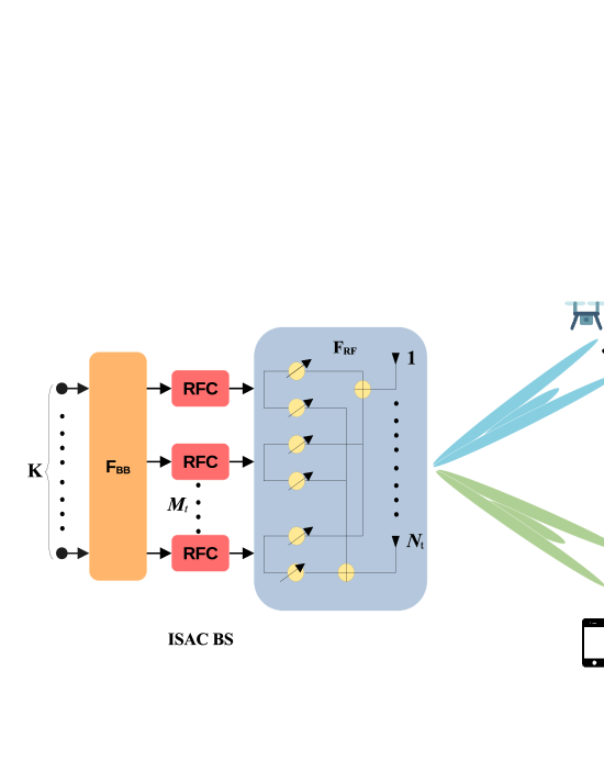
Figure 1: Illustration of an ISAC enabled mmWave MIMO system.

As shown in Fig. 1, we consider an ISAC-aided mmWave MIMO system, where the ISAC BS with $N_{\mathrm{t}}$ transmit antennas/ receive antennas transmits $K=L+M$ streams to serve $M$ users and detect $L$ different radar targets, simultaneously. Moreover, each user is assumed to be equipped with a single antenna. A fully connected hybrid architecture is assumed to be exploited at the ISAC BS with only $M_{\mathrm{t}}<<N_{\mathrm{t}}$ RFCs to reduce the cost and power consumption [mmWave_MIMO_RIS]. Notably, for the considered model, $M_{\mathrm{t}}$ and $K$ are required to satisfy the property $M_{\mathrm{t}}\triangleq K$ at the ISAC BS in order to form $L$ beams for the targets and $M$ beams towards the users. Let us define the transmit signal $\mathbf{x}\in\mathbb{C}^{K\times 1}$ as

$$\mathbf{x}=\bmatrix\mathbf{s}_{1}\\ \mathbf{s}_{2},$$ (1)

where $\mathbf{s}_{1}=[s_{1},s_{2},\hdots,s_{M}]^{T}\in\mathbb{C}^{M\times 1}$ is meant for the users and $\mathbf{s}_{2}=[s_{M+1},\hdots,s_{M_{K}}]^{T}\in{\mathbb C}^{L\times 1}$ is used to detect the targets. Furthermore, we assume that both the signals $\mathbf{s}_{1}$ and $\mathbf{s}_{2}$ are statistically independent with zero mean, i.e., satisfying $\mathbb{E}\{\mathbf{x}\}=\mathbf{0}$ and $\mathbf{E}\{\mathbf{x}\mathbf{x}^{H}\}=\mathbf{I}_{K}$. Following the fully-connected hybrid architecture [mmWave_MIMO_RIS], the transmitted signal $\mathbf{x}$ is first precoded by a BB beamformer $\mathbf{F}_{\mathrm{BB}}=[\mathbf{f}_{{\rm BB},1},\hdots,\mathbf{f}_{{\rm BB},K}]\in{\mathbb C}^{{M_{\mathrm{t}}}\times K}$, followed by precoding using an analog beamformer $\mathbf{F}_{\mathrm{RF}}\in{\mathbb C}^{{N_{\mathrm{t}}}\times{M_{\mathrm{t}}}}$.

II-A Communication model

Considering the availability of the CSI at each user, the received signal $y_{m}$ at the $m$th user can be written as &y_m=h^H_m F_RFF_BBx + n_m,
=h^H_m F_RFf_BB,m s_m + ∑_n=1, n ≠m^Kh^H_mF_RFf_BB,n s_n+ n_m, where the quantity $n_{m}$ is the noise that has the distribution $n_{m}\sim\mathcal{CN}(0,\sigma^{2})$ and $\mathbf{h}_{m}$ is the narrowband block-fading mmWave MISO channel between the ISAC BS and $m$th user, which is given by the model

$$\mathbf{h}^{H}_{m}=\sum_{i=1}^{N^{\rm p}_{m}}\alpha_{m,i}\mathbf{a}_{\rm t}^{H}(\theta_{m,i}),$$ (2)

where $N^{p}_{m}$ denotes the number of multipath components in $\mathbf{h}_{m}$. The quantity $\alpha_{m,i}$ is the channel gain of the $i$th multipath component with distribution $\mathcal{CN}(0,\beta_{m}^{2}10^{-0.1PL(d_{m})}),\forall l=\{1,\hdots,N^{p}_{m}\}$, where $\beta_{m}=\sqrt{N_{\mathrm{t}}/N^{p}_{m}}$ denotes the normalization factor with $PL(d_{m})$ as the path loss that depends on the distance $d_{m}$ associated with the corresponding link. Furthermore, $\mathbf{a}_{\mathrm{t}}(\theta_{l})\in\mathbb{C}^{N_{\mathrm{t}}\times 1}$ is the steering vector of direction $\theta_{l}$, which is given by

$$\aligned\mathbf{a}_{t}\left(\theta_{l}\right)=\frac{1}{\sqrt{N_{t}}}\Biggl{[}1,\ldots,e^{j\frac{2\pi}{\lambda}b\left(n\cos\theta_{l}\right)},\ldots,e^{j\frac{2\pi}{\lambda}b\left({N_{t}-1)\cos\theta_{l}}\right)}\Biggr{]}^{T},$$ (3)

where, $\lambda$ denotes the wavelength and $b$ represents the antenna spacing, which is assumed to be half of the wavelength.

To simplify the notation, we further define

$$\mathbf{F}\triangleq[\mathbf{f}_{1},\mathbf{f}_{2},\ldots,\mathbf{f}_{K}]\triangleq\mathbf{F}_{\mathrm{RF}}\mathbf{F}_{\mathrm{BB}}~{}\in\mathbb{C}^{N_{\mathrm{t}}\times K},$$ (4)

where $\mathbf{f}_{n}\in\mathbb{C}^{N_{\mathrm{t}}\times 1},n=1,2,\hdots,K$ denotes the $n$th column of $\mathbf{F}$. Thus, the SINR of the $m$th user is given by

$$\gamma_{m}\left(\mathbf{F}\right)=\frac{\left|\mathbf{h}^{H}_{m}\mathbf{f}_{m}\right|^{2}}{\sum_{n=1,n\neq m}^{K}{\left|\mathbf{h}_{m}^{H}\mathbf{f}_{n}\right|^{2}}+\sigma^{2}}.$$ (5)

Based on (5), the achievable rate ${\cal R}_{m}$ of the $m$th user is given by

$${\cal R}_{m}\left(\mathbf{F}\right)=\log_{2}\big{(}1+\gamma_{m}\left(\mathbf{F}\right)\big{)}.$$ (6)

II-B Radar model

We consider the same antenna array to be used at the ISAC BS to transmit and receive radar signals. The resulting signal leakage can be overcome efficiently via the correlation suppression techniques, discussed in [CST]. Thus, the received radar signal $\mathbf{y}_{rad}(\theta_{n})\in\mathbb{C}^{N_{\mathrm{t}}\times 1}$ at the ISAC BS can be written as

$$\mathbf{y}_{rad}(\theta_{n})=\mathbf{r}_{t}+\mathbf{r}_{i}+\mathbf{n}_{r},$$ (7)

where $\mathbf{r}_{t},\mathbf{r}_{i}$ and $\mathbf{n}_{r}$ denote the desired target, interference and the noise signals in the radar sensing environment, respectively. It must be noted that some of the targets may act as scatterers for communication. The desired target signal $\mathbf{r}_{t}$ from the $L$ targets is modeled as

$$\mathbf{r}_{t}=\sum_{l=1}^{L}\tau_{l}\mathbf{a}_{\mathrm{t}}(\theta_{l})\mathbf{a}_{\mathrm{t}}^{T}(\theta_{l})\mathbf{F}\mathbf{s},\vspace{-2mm}$$ (8)

where $\tau_{l}$ is the reflection coefficient for a target located at an angle $\theta_{l}$. In order to detect multiple targets, the ISAC BS scans different angles of the space by generating multiple beams toward the targets. To evaluate the sensing performance, we compute the beampattern gains of the targets. Mathematically, the beampattern gain of the target located at $\theta_{l}$ is given as

$$G(\theta_{l},\mathbf{F})=\mathbb{E}\left\{\left|\mathbf{a}_{\mathrm{t}}^{H}(\theta_{l})\mathbf{F}\mathbf{x}\right|^{2}\right\}=\mathbf{a}_{\mathrm{t}}^{H}(\theta_{l})\mathbf{F}\mathbf{F}^{H}\mathbf{a}_{\mathrm{t}}(\theta_{l}).$$ (9)

II-C Energy model

To evaluate the performance of the communication users, we evaluate the EE of the system in bits/Hz/J, which is defined as the ratio of achievable sum-rate to power consumption. Thus, the EE can be expressed as

$$\aligned EE(\mathbf{F})&=\frac{\sum_{m=1}^{M}\mathcal{R}_{m}\left(\mathbf{F}\right)}{P_{\rm diss}\left(\mathbf{F}\right)},$$ (10)

where $P_{\mathrm{diss}}\left(\mathbf{F}\right)$ is the power dissipation for the considered downlink system. This is given by [EE_1, EE_2]

$$\aligned P_{\rm diss}\left(\mathbf{F}\right)=\eta&\sum_{n=1}^{K}\|\mathbf{f}_{n}\|^{2}+M_{\mathrm{t}}P_{\rm c},$$ (11)

where $\eta\in[0,1]$ is the power amplifier efficiency and $P_{\rm c}$ denotes the static hardware power required for each RFC.

II-D Problem formulation

In this work, we aim to optimize the hybrid beamformers $\mathbf{F}_{\mathrm{RF}}$ and $\mathbf{F}_{\mathrm{BB}}$ at the ISAC BS, which maximize the EE of the system $EE(\mathbf{F})$. We consider the SINR requirement of each individual user, beampattern gains of the radar targets and total transmit power as constraints. Therefore, the pertinent optimization problem is given by & max_F∑m=1MRm(F)Pdiss(F)
s.t.  γ_m (F) ≥τ_m,  m=1, 2, , M,
  G(θ_l, F) ≥Γ_l,  l=1, 2, , L,
  ∑_n=1^K∥f_n∥^2≤P_t, where $\tau_{m}$ denotes the required SINR threshold of the $m$th user, $\Gamma_{l}$ is the beampattern gain threshold for the successful sensing of the $l$th target and $P_{\mathrm{t}}$ is the maximum transmit power at the ISAC BS. The above problem (II-D) is highly non-convex, particularly due to the non-concave nature of the objective function (II-D) and the non-convex constraints (II-D).

III Proposed Solution

We employ the well-known Dinkelbach’s method [Dink_1] to deal with the non-concavity of (II-D), which converts a fractional objective function into a subtractive form. To this end, we introduce the quantity $\lambda^{\star}$ as the optimal price corresponding to the optimal fully-digital beamformer $\mathbf{F}^{\star}$. Therefore, the objective function (II-D) can be written in terms of $\lambda^{\star}$ as

$$\lambda^{\star}=\frac{\sum_{m=1}^{M}\mathcal{R}_{m}(\mathbf{F}^{\star})}{P_{\rm diss}(\mathbf{F}^{\star})}=\max_{\mathbf{F}}\frac{\sum_{m=1}^{M}\mathcal{R}_{m}(\mathbf{F})}{P_{\rm diss}(\mathbf{F})}.$$ (12)

As a result, the original fractional problem (II-D) can be reformulated in the subtractive form &max_F∑_m=1^MR_m(F)-λP_diss(F)
s.t.  (II-D),   (II-D)   and  (II-D), where $\lambda>0$ regulates the performance of the system between the achievable sum-rate and the EE. When $\lambda=0$, (III) reduces to sum-rate maximization, since the price associated with power dissipation $P_{\rm diss}$ is zero. Whereas, increasing the value of $\lambda$ results in selecting the available power resources wisely to maximize the EE of the system.

The optimization problem (III) is still non-convex due to the non-convex quantity $\mathcal{R}_{m}(\mathbf{F})$ and the non-convex constraints in (II-D). Therefore, it is challenging to find a closed-form solution using conventional methods. In order to overcome this hurdle, we follow the MMSE-based approach described in [Dink_2]. Employing the available CSI at the ISAC BS, the quantity $\gamma_{m}\left(\mathbf{F}\right)$ can be rewritten as

$$\gamma_{m}\left(\mathbf{F}\right)=\mathbf{f}^{H}_{m}\mathbf{h}_{m}\boldsymbol{\Phi}^{-1}\mathbf{h}^{H}_{m}\mathbf{f}_{m},$$ (13)

where $\boldsymbol{\Phi}=\sum_{n=1,n\neq m}^{K}\mathbf{f}_{n}\mathbf{h}^{H}_{m}\mathbf{h}_{m}\mathbf{f}^{H}_{n}+\sigma^{2}\mathbf{I}$. Thus, the SINR $\gamma_{m}\left(\mathbf{F}\right)$ in (5) can be expressed as $\gamma_{m}(\mathbf{F})=\mathbf{f}^{H}_{m}\mathbf{Q}\mathbf{f}_{m},\forall m$, where $\mathbf{Q}=\mathbf{h}_{m}\boldsymbol{\Phi}^{-1}\mathbf{h}^{H}_{m}$. Hence, the problem (III) can be recast as &max_F ∑_m=1^Mlog_2(1+f^H_mQf_m)-λ∑_n=1^K∥f_n∥^2
s.t.  f^H_mQf_m ≥τ_m, ∀m,   (II-D)   and  (II-D). Furthermore, we define the Hermitian positive semidefinite matrix $\mathbf{T}_{m}=\mathbf{f}_{m}\mathbf{f}^{H}_{m}$ that has rank $1$. Therefore, (III) can be reformulated as &max_T_m ∑_m=1^Mlog_2(1+Tr(QT_m))-λ∑_n=1^KTr(T_n)
s.t.   Tr(QT_m)≥τ_m, ∀m,   (II-D)   and  (II-D). We now relax the rank one constraint of $\mathbf{T}_{m}$ to obtain the semidefinite program (SDP) below max_T_m⪰0 &∑_m=1^Mlog_2(1+Tr(QT_m))-λ∑_n=1^KTr(T_m)
s.t.   Tr(QT_m)≥τ_m, ∀m,   (II-D)   and  (II-D). Note that the above SDP is convex and can be efficiently solved within polynomial time via standard interior-point methods [Dink_2]. Moreover, it should be noted that the solution provided by the SDP (III) is a sub-optimal solution of the original optimization problem (III). However, one can find the rank-one solution by employing eigenvalue decomposition and then choosing the eigenvector corresponding to the maximum eigenvalue as the $m$th beamformer [Dink_2]. Next, we obtain the optimal value of the price factor $\lambda$ by employing a local maximizer of problem (III) as

$$\aligned\lambda^{\star}=\frac{\sum_{m=1}^{M}\mathcal{R}_{m}(\mathbf{F}^{\star})}{P_{\rm diss}.(\mathbf{F}^{\star})}.$$ (14)

[t] Energy-efficient hybrid beamformer design for an ISAC mmWave MIMO system