Excluding the Irrelevant: Focusing Reinforcement Learning through Continuous Action Masking

Abstract

Continuous action spaces in reinforcement learning (RL) are commonly defined as interval sets. While intervals usually reflect the action boundaries for tasks well, they can be challenging for learning because the typically large global action space leads to frequent exploration of irrelevant actions. Yet, little task knowledge can be sufficient to identify significantly smaller state-specific sets of relevant actions. Focusing learning on these relevant actions can significantly improve training efficiency and effectiveness. In this paper, we propose to focus learning on the set of relevant actions and introduce three continuous action masking methods for exactly mapping the action space to the state-dependent set of relevant actions. Thus, our methods ensure that only relevant actions are executed, enhancing the predictability of the RL agent and enabling its use in safety-critical applications. We further derive the implications of the proposed methods on the policy gradient. Using Proximal Policy Optimization (PPO), we evaluate our methods on three control tasks, where the relevant action set is computed based on the system dynamics and a relevant state set. Our experiments show that the three action masking methods achieve higher final rewards and converge faster than the baseline without action masking.

1 Introduction

RL can solve complex tasks in robotics [9], games [27], and is used for fine-tuning large language models [19]. Yet, training reinforcement learning (RL) agents is often sample-inefficient due to frequent exploration of actions, which are irrelevant to learning a good policy. Examples for irrelevant actions are driving into a wall for autonomous cars, or tipping a drone off-balance. The global action space is typically large in relation to the relevant actions in each state. Therefore, exploring these actions frequently can introduce unnecessary costs, lead to slow convergence, or even prevent the agent from learning a suitable policy.

Action masking mitigates this problem by constraining the exploration to the set of relevant state-specific actions, which can be obtained based on task knowledge. For example, when there is no opponent within reach in video games, attack actions are masked from the action space [33]. Leveraging task knowledge through action masking usually leads to faster convergence and also increases the predictability of the RL agent as the set of relevant actions can provide additional meaning. For instance, if the set of relevant actions is a set of verified safe actions, action masking can be used to provide safety guarantees [6, 14].

Whenever the relevant action set is easy to compute, action masking can be seamlessly integrated into RL algorithms and is the quasi-standard for discrete action spaces [36, 26], e.g., in motion planning [18, 13, 32, 22, 4], games [11, 33, 10], and power systems [30, 16]. However, real-world systems operate in continuous space and discretization to a higher-level decision space might prevent learning optimal policies. Furthermore, simulation of real-world systems is compute-intensive, and developing RL agents for them often requires additional real-world training [35]. Thus, sample efficiency is particularly valuable for these applications.

In this work, we propose three action masking methods for continuous action spaces. They employ expressive convex set representations, i.e., polytopes or zonotopes for the relevant action set. Our action masking methods generalize previous work in [14], which is constrained to intervals as relevant action sets. This extends the applicability of continuous action masking to expressive convex relevant action sets, which is especially useful when action dimensions are coupled, e.g., for a thrust-controlled quadrotor. To integrate the relevant action set into RL, we introduce three methods: the generator mask, which exploits the generator representation of a zonotope, the ray mask, which projects an action into the relevant action set based on radial directions, and the distributional mask, which truncates the policy distribution to the relevant action set. In summary our main contributions are:

• We introduce continuous action masking based on arbitrary convex sets representing the state-dependent relevant action sets;

• We present three methods to utilize the relevant action sets and derive their integration in the backward pass of RL with stochastic policies;

• We evaluate our approach on three benchmark environments that demonstrate the application conditions of our continuous action masking approaches.

1.1 Related literature

Action masking is mainly applied for discrete action spaces [6, 18, 13, 32, 22, 4, 11, 33, 10, 30, 16, 14, 36, 31]. Huang et al. [11] derive the implications on policy gradient RL while evaluating the theoretical findings on real-time strategy games. The authors show that masking actions leads to higher training efficiency and scales better with increased action spaces compared to simply penalizing the agent whenever an irrelevant action is selected. Huo et al. [10] extend [11] to off-policy RL and observe similar empirical results.

Action masking for discrete action spaces can be categorized by the purpose of the state-dependent relevant action set. Often, the set is obtained by removing irrelevant actions based on task knowledge [11, 10, 32, 22, 4, 16]. For example, actions that would exceed the maximum speed of an areal vehicle [4]. The relevant action sets are then usually manually engineered. In contrast, a recent study [36] identifies redundant actions based on similarity metrics and removes them automatically to obtain the relevant action set. Another common interpretation of the relevant action set is that it only includes safe actions [18, 13, 30, 6, 31]. Here, the system dynamics are typically used to verify the safety of actions. Safety is either defined as avoiding unsafe areas or complying with logic formulas. In our experiments, we use the former approach to obtain a relevant (safe) action set.

For continuous action spaces, there is only work on utilizing action masking with intervals as relevant action sets [14]. In particular, the proposed continuous action masking uses a safe action interval set as relevant action set and maps the action space to this set with a straightforward re-normalization operation. In this paper, we generalize previous work for more expressive relevant action sets and demonstrate the applicability to three benchmark environments. Note that the ray mask and generator mask are mathematically equivalent to the approach in [14] if the relevant action set is constrained to interval sets.

2 Preliminaries

As basis for our derivations of the three masking methods, we provide a concise overview of RL with policy gradients. Further, we define the system dynamics of the RL environment as well as set representations, which will be used to compute the relevant action set.

2.1 Reinforcement learning with policy gradients

Given a Markov-Decision Process $\left(\mathcal{S},\mathcal{A},T,r,\gamma\right)$, the goal of RL is to learn a parameterized policy $\pi_{\theta}(a|s)$ that maximizes the expected reward $\max_{\theta}\mathbb{E}_{\pi_{\theta}}\sum_{t}\gamma^{t}r(s_{t},a_{t})$, where $r\rightarrow:\mathcal{S}\times\mathcal{A}$ is the reward the agent receives and $\gamma$ is the discount factor for future rewards [29]. The action set $\mathcal{A}$, and state set $\mathcal{S}$ are observable and continuous, and the state-transition function $T(s,a,s^{\prime})$ is stationary.

For policy gradient algorithms, learning the optimal policy $\pi_{\theta}^{*}(a|s)$ is achieved by updating its parameters $\theta$ with the policy gradient

$$\nabla J(\pi_{\theta})=\mathbb{E}_{\pi_{\theta}}\left[\nabla_{\theta}\log\pi_{\theta}(a|s)A_{\pi_{\theta}}(a,s)\right],$$ (1)

where $A_{\pi_{\theta}}(a,s)$ is the advantage function, which represents the expected improvement in reward by taking action $a$ in state $s$ compared to the average action taken in that state according to the policy $\pi_{\theta}(a|s)$ [28]. An estimation of the advantage $A_{\pi_{\theta}}(a,s)$ is usually approximated by a neural network.

2.2 System model and set representations

We consider general continuous-time systems of the form

$$\dot{s}=f(s,a,w),$$ (2)

where $s\in\mathcal{S}\subset\mathbb{R}^{n^{\mathcal{S}}}$, $a\in\mathcal{A}\subset\mathbb{R}^{N}$, and $w\in\mathcal{W}\subset\mathbb{R}^{n^{\mathcal{W}}}$ denote the system state, input, and disturbance, respectively. Input and disturbance are piece-wise constant with a sampling interval $\Delta t$. We assume $\mathcal{S}$, $\mathcal{A}$, and $\mathcal{W}$ to be convex.

A convex set representation well-suited for representing the relevant action set are zonotopes due to the efficiency of operations on them. A zonotope $\mathcal{Z}\subset\mathbb{R}^{N}$ with center $c\in\mathbb{R}^{N}$, generator matrix $G\in\mathbb{R}^{N\times P}$, and scaling factors $\beta\in\mathbb{R}^{P}$ is defined as

$$\mathcal{Z}=\left\{c+G\beta\,\big{|}\,\|\beta\|_{\infty}\leq 1\right\}=\mathcal{Z}(c,G)=\langle c,G\rangle_{\mathcal{Z}}.$$ (3)

The Minkowski addition $\mathcal{Z}_{1}\oplus\mathcal{Z}_{2}$ of two zonotopes $\mathcal{Z}_{1}$, $\mathcal{Z}_{2}$ and the linear map $M\mathcal{Z}_{1}$ of a zonotope $\mathcal{Z}_{1}$ are given by

$$\mathcal{Z}_{1}\oplus\mathcal{Z}_{2} =\langle c_{1}+c_{2},\begin{bmatrix}G_{1}&G_{2}\end{bmatrix}\rangle_{\mathcal{Z}},$$ (4a)

$$M\mathcal{Z}_{1} =\langle Mc_{1},MG_{1}\rangle_{\mathcal{Z}}.$$ (4b)

3 Continuous action masking

To apply action masking, a relevant action set $\mathcal{A}^{r}(s)\subset\mathbb{R}^{N}$ has to be available. For our continuous action masking methods, we specifically require the following two assumptions:

Assumption 1.

The relevant action set $\mathcal{A}^{r}(s)$ is convex and the center and boundary points are computable.

Assumption 2.

The policy $\pi_{\theta}:S\times\mathcal{A}\rightarrow\mathbb{R}_{+}$ of the agent is represented by a parameterized probability distribution $a\sim\pi_{\theta}(a|s)=\mathbb{P}_{\theta}(a;\theta)$.

Common convex set representations that fulfill Assumption 1 are polytopes or zonotopes, which can express a variety of geometric shapes. Our continuous action masking methods transform the policy $\pi_{\theta}(a|s)$, for which the parameters $\theta$ usually specify a neural network, into the relevant policy $\pi_{\theta}^{r}:S\times\mathcal{A}^{r}\rightarrow\mathbb{R}_{+}$ through an abstract mapping function $\mathcal{F}$

$$a^{r}\sim\pi_{\theta}^{r}(a^{r}|s)=\mathcal{F}\big{(}\pi_{\theta}(a|s)\big{)},$$ (5)

so that $a^{r}\in\mathcal{A}^{r}$ always holds. The policy gradient updates only necessitate the ability to sample from, and compute the gradient of the policy, hence $\pi_{\theta}^{r}(a^{r}|s)$ does not have to be available in closed form.

In the following, we introduce and evaluate three mapping methods: generator mask, ray mask, and distributional mask, as shown in Fig. 1. Note that by ensuring only actions in the relevant action set $\mathcal{A}^{r}(s)$ are selected, all three methods potentially increase the predictability and safety of the RL agent. We derive the effect of each mapping approach on the gradient of the agent’s objective function for the most common stochastic policy RL algorithm; PPO.

(a) Ray mask

(b) Generator mask

(c) Distributional mask

Figure 1: Illustration of masking methods in action space $\mathcal{A}$ with a hexagon-shaped relevant action set $\mathcal{A}^{r}$. The ray mask radially maps the actions towards the center of the relevant action set. The generator mask employs the latent action space $\mathcal{A}^{l}$, which is the generator space of the zonotope modeling the relevant action set. The distributional mask augments the policy probability density function so that it is zero outside the relevant action set.

3.1 Ray mask

The ray mask locally compresses the action set $\mathcal{A}$ into $\mathcal{A}^{r}$, which is accomplished by scaling each action $a$ alongside a ray from the center of $\mathcal{A}^{r}$ to the boundary of $\mathcal{A}$ This allows for sets with substantially different shapes, as shown in Figure 1(a). Specifically, the relevant policy distribution is created by transforming the action $a\in\mathcal{A}\subset\mathbb{R}^{N}$, given by $\pi_{\theta}(a|s)$, with a mapping function $g:\mathcal{A}\rightarrow\mathcal{A}^{r}$:

$$a^{r}=g(a)=c+\frac{\lambda_{\mathcal{A}}(a)}{\lambda_{\mathcal{A}^{r}}(a)}(a-c).$$ (6)

Here, $\lambda_{\mathcal{A}}(a)$, and $\lambda_{\mathcal{A}^{r}}(a)$ denote the distances to the boundary of the relevant action set and action space, respectively, measured from the center of the relevant action set $c$ in the direction of $a$. Note that computing $\lambda_{\mathcal{A}^{r}}(a)$ for a zonotope requires solving a convex optimization problem, as specified in Appendix A.4. Yet, the ray mask is applicable for all convex sets, for which we can compute the center and boundary points. Since $g(a)$ is bijective, we can apply the change of variables formula to compute the relevant policy

$$\pi_{\theta}^{r}(a^{r}|s)=\pi_{\theta}\left(g^{-1}(a^{r})|s\right)\left|\text{det}\left(\frac{\mathrm{d}}{\mathrm{d}a^{r}}g^{-1}(a^{r})\right)\right|,$$ (7)

where $g^{-1}(a^{r})=a$ is the inverse of $g$ at $a$. In general, there is no closed form of this distribution available. However, for policy gradient-based RL, we only require to sample from the distribution and compute its policy gradient. Samples from $\pi_{\theta}^{r}(a^{r}|s)$ are created by sampling from the original policy $a\sim\pi_{\theta}(a|s)$, which is transformed with $a^{r}=g(a)$. The policy gradient is derived in the following.

Proposition 1.

Policy gradient for the ray mask.

The policy gradient of $\pi_{\theta}^{r}(a|s)$ for the ray mask is given by

$$\nabla_{\theta}J\left(\pi_{\theta}^{r}(a|s)\right)=\mathbb{E}_{\pi_{\theta}^{r}}\left[\nabla_{\theta}\log\pi_{\theta}(a|s)A_{\pi_{\theta}^{r}}(a^{r},s)\right],$$ (8)

where $A_{\pi_{\theta}^{r}}(a^{r},s)$ is the advantage function associated to $\pi_{\theta}^{r}(a|s)$, and evaluated at the action $a^{r}$.

Proof.

Since the determinant in (7) is independent of $\theta$, the gradient of it w.r.t. $\theta$ is

$$\nabla_{\theta}\text{det}\left(\frac{\mathrm{d}}{\mathrm{d}a^{r}}g^{-1}(a^{r})\right)=0,$$ (9)

which simplifies the score function of $\pi_{\theta}^{r}(a|s)$ to

$$\nabla_{\theta}\log\pi_{\theta}^{r}(a|s)=\nabla_{\theta}\log\pi_{\theta}(a|s).$$ (10)

Combining (10) and the general form of the policy gradient for $\pi_{\theta}^{r}(a|s)$, as in (1), results in (8).

∎

3.2 Generator mask

Zonotopes are a scalable convex set representation. By definition (see Section 2.2), they map a point from the hypercube in the generator space to a point in the set space. The generator mask is based on exploiting this property by letting the RL agent select actions in the generator space. Since the size of the output layer of the policy or Q-function network cannot change during the learning process, we require that the dimensionality of the generator space static. Overall, the generator mask requires the following assumption:

Assumption 3.

The relevant action set $\mathcal{A}^{r}(s)$ is represented by a zonotope and the generator dimensions for the relevant action set are fixed during training and deployment.

In particular, the relevant action set $\mathcal{A}^{r}(s)$ is defined as $\langle c(s),G(s)\rangle_{\mathcal{Z}}$, with $G\in\mathbb{R}^{P\times N}$ and $c\in\mathbb{R}^{N}$. Note that in practice Assumption 3 is typically a weak limitation since a high-dimensional generator space allows for a greater variety of relevant action sets. Since the policy $\pi_{\theta}(a|s)$ is defined in the space of the zonotope’s hypercube, we treat the hypercube as a latent action space $\mathcal{A}^{l}\subset\mathbb{R}^{P}$. However, the domain of $\pi_{\theta}^{r}(a^{r}|s)$ is still a subset of the action space $\mathcal{A}^{r}\subseteq\mathcal{A}\subset\mathbb{R}^{N}$ (see Figure 1(b)).

For deriving the policy gradient of the generator mask, we assume that the policy follows the most common probability distribution for continuous RL policies:

Assumption 4.

$\pi_{\theta}(a|s)$ follows a normal distribution $\mathcal{N}(a;\mu_{\theta},\Sigma_{\theta})$.

Proposition 2.

The relevant policy of the generator mask is given by

$$\pi_{\theta}^{r}(a|s)=\mathcal{N}(a;G\mu_{\theta}+c,G\Sigma_{\theta}G^{T})$$ (11)

Proof.

The mapping function for the generator mask $g:\mathcal{A}\rightarrow\mathcal{A}^{r}$, as defined by the mapping of a zonotope,

$$a^{r}=g(a)=c+Ga,$$ (12)

represents a linear mapping of $a\sim\pi_{\theta}(a|s)$. Therefore, we can apply the linear transformation theorem for multivariate normal distributions, to compute the closed-form of the relevant policy in (11) (see Lemma 1 in Appendix A.1). ∎

Next, we discuss the implications of this mapping on the policy gradient. Since $g(a)$ is not bijective generally, we cannot derive the gradient through the change of variables formula as for the ray mask.

Proposition 3.

The policy gradient for $\pi_{\theta}^{r}(a^{r}|s)$ as defined in (11) with respect to $\mu_{\theta}$ and $\Sigma_{\theta}$ is given by

$$\nabla_{\mu_{\theta}}\log\pi_{\theta}^{r}(a^{r}|s)= \,G^{T}(G\Sigma_{\theta}G^{T})^{-1}(a^{r}-c-G\mu_{\theta}),$$ (13)

$$\nabla_{\Sigma_{\theta}}\log\pi_{\theta}^{r}(a^{r}|s)= \,-\frac{1}{2}\big{(}G^{T}(G\Sigma_{\theta}G^{T})^{-1}G-G^{T}(G\Sigma_{\theta}G^{T})^{-1}(a^{r}-c-G\mu_{\theta})$$ (14)

$$(a^{r}-c-G\mu_{\theta})^{T}(G\Sigma_{\theta}G^{T})^{-1}G\big{)}.$$

Proof.

The proposition is proven with linear algebra operations and detailed in Appendix A.2. ∎

Note that the expressions in (13) and (14) simplify to $\nabla_{\mu_{\theta}}\log\pi_{\theta}(a|s)$, and $\nabla_{\Sigma\theta}\log\pi_{\theta}(a|s)$, respectively, if $G^{-1}$ exists, i.e., $G$ is square and non-singular (see Proposition 5 in Appendix A.2).

3.3 Distributional mask

The intuition behind the distributional mask is drawn from discrete action masking, where the probability for irrelevant actions is set to $0$ [11]. For continuous action spaces, we aim to achieve the same by ensuring that actions are only sampled from the relevant action set $\mathcal{A}^{r}(s)$, by constraining the policy distribution $\pi_{\theta}(a|s)$ to this convex set (see Figure 1(c)). For the one-dimensional case, this can be expressed by the truncated distribution. In higher dimensions, the resulting policy density is

$$\pi_{\theta}^{r}(a^{r}|s)=\frac{\phi(a,s)\pi_{\theta}(a|s)}{\int_{\mathcal{A}^{r}}\pi_{\theta}(a|s)\mathrm{d}a},$$ (15)

where $\phi(a,s)$ is the indicator function

$$\phi(a,s)=\begin{cases}1&\text{if }a\in\mathcal{A}^{r}(s),\\ 0&\text{otherwise}.\end{cases}$$ (16)

Since there is no closed-form of this density, we employ Markov-Chain Monte-Carlo sampling to sample actions from the policy. More specifically, we utilize the random direction Hit-and-Run algorithm: a geometric random walk that allows sampling from a non-negative, integrable function $f:\mathbb{R}^{N}\rightarrow\mathbb{R}_{+}$, while constraining the samples to a bounded set [34]. The algorithm iteratively chooses a random direction from the current point, computes the one-dimensional, truncated probability density of $f$ along this direction, and samples a new point from this density. The approach is particularly effective for high-dimensional spaces where other sampling methods might struggle with convergence or efficiency. For the distributional mask, $f$ is the policy $\pi_{\theta}(a|s)$, and the set is $\mathcal{A}^{r}(s)$. As suggested by [17], we choose the mixing time to be $N^{3}$, i.e., we execute $N^{3}$ iterations before accepting the sample. To estimate the integral in (15), we use numerical integration with cubature [7], which is a method to approximate the definite integral of a function $h:\mathbb{R}^{N}\rightarrow\mathbb{R}$ over a multidimensional geometric set.

Proposition 4.

The policy gradient for the distributional mask is

$$\nabla_{\theta}\log\pi_{\theta}^{r}(a^{r}|s)=\nabla_{\theta}\log\pi_{\theta}(a|s)-\nabla_{\theta}\log\int_{\mathcal{A}^{r}}\pi_{\theta}(a|s)\mathrm{d}a.$$ (17)

Proof.

The indicator function, $\pi_{\theta}^{r}(a^{r}|s)$ is not continuous and differentiable, which necessitates the use of the sub-gradient for learning. However, since $a^{r}\in\mathcal{A}^{r}$ always holds, the gradient has to be computed for the continuous part of $\pi_{\theta}^{r}(a^{r}|s)$ only, and thus $\phi(a,s)$ can be omitted. ∎

Since we cannot compute the gradient of the numerical integral $\int_{\mathcal{A}^{r}}\pi_{\theta}(a|s)\mathrm{d}a$, we treat the integral as a constant in practice, and approximate $\nabla_{\theta}\log\pi_{\theta}^{r}(a^{r}|s)\approx\nabla_{\theta}\log\pi_{\theta}(a|s)$. We discuss potential improvements in Section 4.3.

4 Numerical experiments

We compare the three continuous action masking methods on three different environments: The simple and intuitive Seeker Reach-Avoid environment, the 2D Quadrotor environment to demonstrate the generalization from the continuous action masking approach in [14], and the 3D Quadrotor environment to show the applicability to higher dimensional action spaces. Because the derivation of the relevant action set is not trivial in practice, we selected three environments for which we could compute intuitive relevant action sets. We use the stable-baseline3 [21] implementation of PPO [25]. PPO is selected for the experiments, because it is a widely-used algorithm in the field of reinforcement learning and fulfills both Assumptions 2 and 4 per default. We conduct a hyperparameter optimization with $50$ trials for each masking method and environment. The resulting hyperparameters are reported in Appendix A.7. All experiments are run on a machine with a Intel(R) Xeon(R) Platinum 8380 2.30 GHz processor and 2 TB RAM.

4.1 Environments

We briefly introduce the three environments with their dynamics, state space, action space, reward, and relevant action set $\mathcal{A}^{r}(s)$. Parameters for the environments are detailed in Appendix A.5.

4.1.1 Seeker Reach-Avoid

This episodic environment features an agent navigating a 2D space, tasked with reaching a goal while avoiding a circular obstacle (see Figure 2). It is explicitly designed to provide an intuitive relevant action set $\mathcal{A}^{r}$. The system is defined as in Section 2.2: The dynamics for the agent position $s=\left[s_{x},s_{y}\right]$ and the action $a=\left[a_{x},a_{y}\right]$ are $\dot{s}=a$, and there are no disturbances.

Figure 2: The Seeker Reach-Avoid environment with examplatory state space configuration (left) and action space (middle). The agent (black) has to reach the goal (gray), while avoiding the obstacle (red). The center of the action space is illustrated with a black dot and the relevant action set $\mathcal{A}^{r}$ for the current state is shown in green. The state set at the next time step $k+1$ reachable with the relevant action set is $\mathcal{S}_{k+1}$.

The environment is characterized by the agent’s position, the goal position $s^{*}$, the obstacle position $o$, and the obstacle radius $r_{o}$. These values are pseudo-randomly assigned at the beginning of each episode, with the constraints that the goal cannot be inside the obstacle and the obstacle blocks the direct path between the agent’s initial position and the goal. The reward for each time step is

$$r(a,s)=\begin{cases}100&\text{if goal reached},\\ -100&\text{if collision occurred},\\ -1-||s^{*}-s||_{2}&\text{otherwise}.\end{cases}$$ (18)

We compute the relevant action set $\mathcal{A}^{r}(s)$ so that all actions that cause a collision with the obstacle or the boundary, are excluded (see Appendix A.3.3).

4.1.2 2D Quadrotor

The 2D Quadrotor environment models a stabilization task and employs an action space where the two action dimensions are coupled, i.e., rotational movement is originating from differences between the action values and vertical movement is proportional to the sum of the action values. Specifically, the system dynamics are:

$$\dot{s}=\left(\begin{array}[]{c}\dot{x}\\ \dot{z}\\ (a_{1}+a_{2})k\sin(\theta)\\ -g+(a_{1}+a_{2})k\cos(\theta)\\ \dot{\theta}\\ -d_{0}\theta-d_{1}\dot{\theta}+n_{0}(-a_{1}+a_{2})\end{array}\right)+\left(\begin{array}[]{c}0\\ 0\\ w_{1}\\ w_{2}\\ 0\\ 0\end{array}\right),$$ (19)

where the state is $s=\left[x,z,\dot{x},\dot{z},\theta,\dot{\theta}\right]$, the action is $a=\left[a_{1},a_{2}\right]$, and the disturbance is $w=\left[w_{1},w_{2}\right]$. The parameter values are specified in Appendix A.5. The relevant action set is computed based on the system dynamics and a relevant state set (see Appendix, Eq. (35)). The reward function is defined as

$$r(a,s)=\exp\left(-\|s-s^{*}\|_{2}-\frac{0.01}{2}\left\|\frac{a-\mathrm{min}(\mathcal{A})}{\mathrm{max}(\mathcal{A})-\mathrm{min}(\mathcal{A})}\right\|_{1}\right),$$ (20)

where $s^{*}=\mathbf{0}$ is the stabilization goal state, $\mathrm{min}(\mathcal{A})$ returns the lower bound for each dimension of the action space, and $\mathrm{max}(\mathcal{A})$ the upper bound.

4.1.3 3D Quadrotor

The last environment models a stabilization task defined in [12]. The system is modeled in a twelve-dimensional state space with state $s=[x,y,z,\dot{x},\dot{y},\dot{z},\theta,\phi,\psi,\dot{\theta},\dot{\phi},\dot{\psi}]$ and four-dimensional action space with action $a=[a_{1},a_{2},a_{3},a_{4}]$. The system dynamics are $\dot{s}=[\dot{x},\dot{y},\dot{z},-9.81\phi,9.81\theta,a_{1},\dot{\theta},\dot{\phi},\dot{\psi},a_{2},a_{3},a_{4}]$ The reward is defined in (20) As for the 2D Quadrotor environment, we calculate the relevant action set based on the system dynamics and a relevant state set (see Appendix, Eq. (35)).

4.2 Results

The reported training results are based on ten random seeds for each configuration. Figure 3 shows the mean reward and bootstrapped 95% confidence interval [20] for the three environments. For all environments, the baseline, which is standard PPO, converges significantly slower or not at all. Additionally, the initial rewards when using action masking methods are significantly higher than for the baseline, indicating that the exploration is indeed constrained to relevant task-fulfilling actions. We depict the mean and standard deviation of the episode return during deployment in Table 1. The baseline episode returns are significantly lower than for action masking while the three masking methods perform similar.

For the Seeker environment, the fraction between relevant action set and global action space is on average $70\%$. All action masking methods converge significantly faster to high rewards than the baseline. The generator mask and the distributional mask achieve the highest final reward. For the 2D Quadrotor, the relevant action to action space fraction is much smaller with on average $28\%$. In this environment, the ray mask and generator mask achieve the highest reward. While the baseline converges significantly slower, the final average reward is similar to the one of the distributional mask. Note that the confidence interval for the baseline is significantly larger. This is because three of the ten runs do not converge and produce an average reward around one throughout training. Note that if we constrain the relevant action set to an interval for this environment, our optimization problem in (35) often renders infeasible because the maximal relevant action set cannot be well approximated by an interval. Thus, the masking method proposed in [14] is not suitable for the 2D Quadrotor task. The results on the 3D Quadrotor are similar to those on the 2D Quadrotor, again the generator mask converges the fastest but yields a final reward similar to that of the ray mask. The fraction of the relevant action space is on average $25\%$. Notably, on this environment the baseline does not learn a meaningful policy.

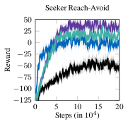
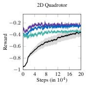
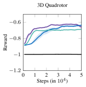
Figure 3: Average reward curves for benchmarks with transparent bootstrapped 95% confidence interval.

Table 1: Mean and standard deviation of episode return for ten runs per trained model.

	Baseline	Ray mask	Generator mask	Distributional mask
Seeker	$-71.03\pm 19.670$	$-20.45\pm 16.39$	$18.60\pm 22.02$	$-13.66\pm 19.97$
2D Quadrotor	$-0.80\pm 0.15$	$-0.26\pm 0.05$	$-0.25\pm 0.02$	$-0.23\pm 0.02$
3D Quadrotor	$-1.00\pm 0.00$	$-0.63\pm 0.03$	$-0.68\pm 0.07$	$-0.66\pm 0.02$

4.3 Limitations

Our experimental results provide indication that continuous action masking with zonotopes can improve both the sample efficiency and the final policy of PPO. While the sample efficiency is higher in our experiments, computing the relevant action set adds additional computational load as apparent from the increased computation times (see Appendix A.6). Thus, in practice a tight relevant action set might increase the computation time by more than the computation time for additional samples with standard RL algorithms. Yet, if the relevant action set provides guarantees, e.g., is a set of verified safe actions, this increased computation time might be acceptable.

PPO is the most common RL algorithm. However, off-policy algorithms such as Twin Delayed DPPG (TD3) [5] and Soft Actor-Critic (SAC) [8] are frequently employed as well. The ray mask and generator mask are conceptually applicable for deterministic policies as used in TD3. Yet, the implications on the gradient must be derived for each RL algorithm and are subject to future work. For the distributional mask, treating the integral in (15) as constant w.r.t. to $\theta$ is a substantial simplification, which might be an explanation of the slightly worse convergence of the distributional mask. To address this in future work, one could approximate the integral with a neural network, which has the advantage that it is easily differentiable.

We focus this work on the integration of a convex relevant action set into RL and assume that an appropriate relevant action set can be obtained. Yet, obtaining this can be a major challenge in practice. On the one hand, the larger the relevant action set is with respect to the action space, the smaller the sample efficiency gain from action masking might get. On the other hand, an accurate relevant action set might require significant computation time to obtain and could lead to a high-dimensional generator space, which could be challenging for the generator mask. Thus, future work should investigate efficient methods to obtain sufficiently tight relevant action sets.

5 Conclusion

We propose action masking methods for continuous action spaces that focus the exploration on the relevant part of the action set. In particular, we extend previous work on continuous action masking to general convex relevant action sets. To this end, we introduce three masking methods and derive their implications on the gradient of PPO. We empirically evaluate the methods on three benchmarks and observe that the generator mask and ray mask perform best. If the relevant action set can be described by a zonotope with fixed generator dimensions and the policy follows a normal distribution, the generator mask is straightforward to implement. If the assumptions for the generator mask cannot be fulfilled, the ray mask is recommended based on our experiments. Because of the subpar performance and longer computation time of the distributional mask, it needs to be further improved. Future work should also investigate a broad range of benchmarks to more clearly identify the applicability and limits of continuous action masking with expressive convex sets.

Appendix A Appendix

A.1 Linear transformation of multivariate normal distributions

Lemma 1.

Applying the linear mapping of a Zonotope $\langle c,G\rangle_{\mathcal{Z}}$ for the multivariate normal distribution $a\sim\mathcal{N}(\mu,\Sigma)$ results in the multivariate normal distribution $b=c+Ga\sim\mathcal{N}(c+G\mu,G\Sigma G^{T}$).

Proof.

The moment-generating function of the random variable $a$ is $M_{a}(t)=\mathbb{E}_{a}\left[\exp\left(t^{T}a\right)\right]$, and for $b$ it is

$$\begin{split}M_{b}(t)&=\mathbb{E}_{a}\left[\exp\left(t^{T}(c+Ga)\right)\right]\\ &=\exp\left(t^{T}c\right)\mathbb{E}_{a}\left[\exp\left(t^{T}Ga\right)\right]\\ &=\exp\left(t^{T}c\right)M_{a}(G^{T}t).\end{split}$$ (21)

Since $a$ is normally distributed, we can write $M_{a}(t)=\exp\left(t^{T}\mu+0.5t^{T}\Sigma t\right)$, and hence

$$\begin{split}M_{b}(t)&=\exp\left(t^{T}c\right)\exp\left(t^{T}G\mu+0.5t^{T}G\Sigma G^{T}t\right)\\ &=\exp\left(t^{T}(G\mu+c)+0.5t^{T}G\Sigma G^{T}t\right),\end{split}$$ (22)

which is the moment-generating function for the variable b $\sim\mathcal{N}(c+G\mu,G\Sigma G^{T})$. ∎

A.2 Policy gradient for the generator mask

The log probability density function of the relevant policy for the generator mask is

$$\log\pi_{\theta}^{r}(a^{r}|s)=-\frac{d}{2}\log(2\pi)-\frac{1}{2}\log|G\Sigma_{\theta}G^{T}|-\frac{1}{2}(a^{r}-c-G\mu_{\theta})^{T}(G\Sigma_{\theta}G^{T})^{-1}(a^{r}-c-G\mu_{\theta}).$$ (23)

We can derive the gradient w.r.t $\mu_{\theta}$ as

$$\begin{split}\nabla_{\mu_{\theta}}\log\pi_{\theta}^{r}(a^{r}|s)&=-\frac{1}{2}\nabla_{\mu_{\theta}}(a^{r}-c-G\mu_{\theta})^{T}(G\Sigma_{\theta}G^{T})^{-1}(a^{r}-c-G\mu_{\theta})\\ &=-\frac{1}{2}\left(-2(G\Sigma_{\theta}G^{T})^{-1}(a^{r}-c-G\mu_{\theta})\right)\nabla_{\mu_{\theta}}(a^{r}-c-G\mu_{\theta})\\ &=G^{T}(G\Sigma_{\theta}G^{T})^{-1}(a^{r}-c-G\mu_{\theta}),\\ \end{split}$$ (24)

and w.r.t $\Sigma_{\theta}$ as

$$\nabla_{\Sigma_{\theta}}\log\pi_{\theta}^{r}(a^{r}|s)=$$

$$=-\frac{1}{2}\nabla_{\Sigma_{\theta}}\log|G\Sigma_{\theta}G^{T}|-\frac{1}{2}\nabla_{\Sigma_{\theta}}(a^{r}-c-G\mu_{\theta})^{T}(G\Sigma_{\theta}G^{T})^{-1}(a^{r}-c-G\mu_{\theta})$$

$$=-\frac{1}{2}(G\Sigma_{\theta}G^{T})^{-1}\nabla_{\Sigma_{\theta}}G\Sigma_{\theta}G^{T}$$ (25)

$$\quad+\frac{1}{2}(G\Sigma_{\theta}G^{T})^{-1}(a^{r}-c-G\mu_{\theta})(a^{r}-c-G\mu_{\theta})^{T}(G\Sigma_{\theta}G^{T})^{-1}\nabla_{\Sigma_{\theta}}G\Sigma_{\theta}G^{T}$$

$$=-\frac{1}{2}\left(G^{T}(G\Sigma_{\theta}G^{T})^{-1}G-G^{T}(G\Sigma_{\theta}G^{T})^{-1}(a^{r}-c-G\mu_{\theta})(a^{r}-c-G\mu)^{T}(G\Sigma_{\theta}G^{T})^{-1}G\right)$$

We can state the following, for the special case, when the inverse of $G$ exists.

Proposition 5.

If $G$ is invertible, $\nabla_{\theta}\log\pi_{\theta}^{r}(a^{r}|s)=\nabla_{\theta}\log\pi_{\theta}(a|s)$ holds for the generator mask.

Proof.

If $G$ is invertible, we can further simplify (24) to

$$\begin{split}\nabla_{\mu_{\theta}}\log\pi_{\theta}^{r}(a^{r}|s)&=G^{T}G^{-T}\Sigma_{\theta}^{-1}G^{-1}(a^{r}-c-G\mu_{\theta})\\ &=\Sigma_{\theta}^{-1}\left(G^{-1}(a^{r}-c)-G^{-1}G\mu_{\theta}\right)\\ &=\Sigma_{\theta}^{-1}\left(a-\mu_{\theta}\right)=\nabla_{\mu_{\theta}}\log\pi_{\theta}(a|s),\end{split}$$ (26)

and (A.2) to

$$\begin{split}\nabla_{\Sigma_{\theta}}\log\pi_{\theta}^{r}(a^{r}|s)&=-\frac{1}{2}\left(\Sigma_{\theta}^{-1}-\Sigma_{\theta}^{-1}G^{-1}(a^{r}-c-G\mu_{\theta})(a^{r}-c-G\mu_{\theta})^{T}G^{-T}\Sigma_{\theta}^{-1}\right)\\ &=-\frac{1}{2}\left(\Sigma_{\theta}^{-1}-\Sigma_{\theta}^{-1}(a-\mu_{\theta})(a-\mu_{\theta})^{T}\Sigma_{\theta}^{-1}\right)=\nabla_{\Sigma_{\theta}}\log\pi_{\theta}(a|s),\end{split}$$ (27)

by using $a=g^{-1}(a^{r})=G^{-1}(a^{r}-c)$, and thus proving the statement. ∎

A.3 Computation of the relevant action set

A.3.1 General case

Given an initial state $s_{0}$, an input trajectory $a$, and a disturbance trajectory $w$, we denote the solution of (2) at time $t$ as $\xi_{t}(s_{0},a,w)$. The reachable set of (2) at some time $t$ given an uncertain initial state $\mathcal{S}_{0}$ and an input trajectory $a$ is denoted as

$$\mathcal{R}^{e}_{t}(\mathcal{S}_{0},a)=\big{\{}\xi_{t}(s_{0},a,w)\colon\exists s_{0}\in\mathcal{S}_{0},\exists w\in\mathcal{W}\big{\}}.$$ (28)

The reachable set over the time interval $[0,t]$ is defined as

$$\mathcal{R}^{e}_{[0,t]}(\mathcal{S}_{0},a)=\bigcup_{\tau\in[0,t]}\mathcal{R}^{e}_{\tau}(\mathcal{S}_{0},a).$$ (29)

For a single time step, we can compute the reachable set given a set of inputs $\tilde{\mathcal{A}}\subseteq\mathcal{A}$ as

$$\mathcal{R}^{e}_{\Delta t}(\mathcal{S}_{0},\tilde{\mathcal{A}})=\big{\{}\xi_{t}(s_{0},a,w)\colon\exists x_{0}\in\mathcal{S}_{0},\exists a\in\tilde{\mathcal{A}},\exists w\in\mathcal{W}\big{\}}.$$ (30)

It can be prohibitively hard to compute the reachable set exactly, which is why we generally compute overapproximations $\mathcal{R}(\cdot)\supseteq\mathcal{R}^{e}(\cdot)$.

To guarantee constraint satisfaction over an infinite time horizon, we use a relevant state set $\mathcal{S}^{r}$. This set is defined such that constraint satisfaction is guaranteed for all time as long as the system state remains inside it. Formally, it is defined such that

$$\forall\mathcal{S}\subseteq\mathcal{S}^{r},\exists a\in\mathcal{A}\colon\mathcal{R}_{\Delta t}(\mathcal{S},a)\subseteq\mathcal{S}^{r},\mathcal{R}_{[0,\Delta t]}(\mathcal{S},a)\subseteq\mathcal{S}.$$ (31)

Such sets are commonly called control invariant. For an efficient computation, the reader is referred to [24].

We compute the relevant action set as the largest set of inputs that allows us to keep the system in the relevant state set in the next step. We define a parameterized action set $\mathcal{A}^{r}(p)$, where $p\in\mathbb{R}^{n^{p}}$ is a parameter vector. The relevant action set at some time step $k$ is then computed with the optimal program

$$\!\max_{p} \text{Vol}\left(\mathcal{A}^{r}_{k}(p)\right)$$ (32)

subject to $$\mathcal{A}^{r}_{k}(p)\subseteq\mathcal{A}$$

$$\mathcal{R}_{k+\Delta t}(\mathcal{S}_{k},\mathcal{A}^{r}_{k}(p))\subseteq\mathcal{S}^{r}$$

$$\mathcal{R}_{[k,k+\Delta t]}(\mathcal{S}_{k},\mathcal{A}^{r}_{k}(p))\subseteq\mathcal{S},$$

where $\texttt{Vol}(\cdot)$ is a function representing the set volume. In the following, we provide a detailed formulation of (32) as an exponential cone program.

A.3.2 Exponential cone program

We consider the discrete-time linearization of our system

$$s_{k+1}=As_{k}+Ba_{k}+w_{k}^{\prime},$$ (33)

where $w_{k}^{\prime}\in\mathcal{W}^{\prime}(s_{k})$ additionally contains linearization errors and the enclosure of all possible trajectory curvatures between the two discrete time steps [2]. Furthermore, we assume $\mathcal{S}$, $\mathcal{A}$, $\mathcal{W}$, and $\mathcal{S}^{r}$ to be zonotopes.

With regard to the input set parameterization, we consider a template zonotope with a predefined template generator matrix $\tilde{G}$ and variable generator scaling factors. We then use the vector $p^{G}\in\mathbb{R}^{n^{g}}_{>0}$ of generator scaling factors to define the generator matrix. The parameterized template zonotope is then given by

$$\mathcal{A}^{r}(p)=c+\tilde{G}\,diag(p^{G}),$$ (34)

where $p=\begin{bmatrix}c&p^{G}\end{bmatrix}^{\top}$.

We denote the center and generator matrix of a zonotope $\mathcal{Z}$ by $c^{\mathcal{Z}}$ and $G^{\mathcal{Z}}$, respectively. Based on the linearized system dynamics, and using $\mathcal{R}$ as a shorthand for $\mathcal{R}_{k+\Delta t}(\cdot)$, we have $G^{\mathcal{R}}=\begin{bmatrix}AG^{\mathcal{S}_{0}}&BG^{\mathcal{A}^{r}_{k}}&G^{\mathcal{W}}\end{bmatrix}$ and $c^{\mathcal{R}}=\begin{bmatrix}Ac^{\mathcal{S}_{0}}&Bc^{\mathcal{A}^{r}_{k}}&c^{\mathcal{W}}\end{bmatrix}$.

We follow the approach in [23] to formulate the set containment constraints in (32) as linear constraints. Since we already consider trajectory curvature in the disturbance, we only need to guarantee that the relevant input set is contained in the feasible input set and that the reachable set of the next time step is contained in the relevant state set. We define the auxiliary variables $\Gamma^{\mathcal{R}}\in\mathbb{R}^{n^{\mathcal{S}^{r}}\times n^{\mathcal{R}}}$, $\beta^{\mathcal{R}}\in\mathbb{R}^{n^{\mathcal{S}^{r}}}$, $\Gamma^{\mathcal{A}^{r}_{k}}\in\mathbb{R}^{n^{\mathcal{A}}\times n^{\mathcal{A}^{r}_{k}}}$, and $\beta^{\mathcal{A}^{r}_{k}}\in\mathbb{R}^{n^{\mathcal{A}}}$ and solve

$$\!\max_{p} \text{Vol}\left(\mathcal{A}^{r}_{k}(p)\right)$$ (35)

subject to $$G^{\mathcal{R}}-G^{\mathcal{S}^{r}}\Gamma^{\mathcal{R}}=\mathbf{0}$$

$$c^{\mathcal{S}^{r}}-c^{\mathcal{R}}-G^{\mathcal{S}^{r}}\beta^{\mathcal{R}}=\mathbf{0}$$

$$\|\begin{bmatrix}\Gamma^{\mathcal{R}}&\beta^{\mathcal{R}}\end{bmatrix}\|_{\infty}\leq 1$$

$$G^{\mathcal{A}^{r}_{k}}-G^{\mathcal{A}}\Gamma^{\mathcal{A}^{r}_{k}}=\mathbf{0}$$

$$c^{\mathcal{A}}-c^{\mathcal{A}^{r}_{k}}-G^{\mathcal{A}}\beta^{\mathcal{A}^{r}_{k}}=\mathbf{0}$$

$$\|\begin{bmatrix}\Gamma^{\mathcal{A}^{r}_{k}}&\beta^{\mathcal{A}^{r}_{k}}\end{bmatrix}\|_{\infty}\leq 1,$$

where $\mathbf{0}$ are zero matrices of appropriate dimensions. By vectorizing $\Gamma^{\mathcal{R}}$ and $\Gamma^{\mathcal{A}^{r}_{k}}$ and resolving the absolute value constraints, we can obtain a formulation with purely linear constraints. Since computing the exact volume of a zonotope is computationally expensive, we approximate it by computing the geometric mean of the parameterization vector:

$$\texttt{Vol}(\mathcal{A}^{r}_{k}(p))=\left(\prod_{i}p_{i}\right)^{\frac{1}{n^{p}}}.$$ (36)

With the cost function from (36), the problem in (35) represents an exponential cone program, which is convex and can be efficiently computed [3].

A.3.3 Seeker Reach-Avoid environment

Because of the dynamics of the seeker reach-avoid environment, we can simplify the relevant action set computation to the following optimization problem

$$\!\max_{p} \text{Vol}(\mathcal{A}^{r}_{k}(p))$$ (37)

subject to $$\mathcal{A}^{r}_{k}(p)\subseteq\mathcal{A}$$

$$\mathcal{S}^{r}_{k+\Delta t}=s_{k}\oplus\mathcal{A}^{r}_{k}(p)$$

$$\mathcal{S}^{r}_{k+\Delta t}\subseteq\left[-10,10\right]^{2}$$

$$\mathcal{S}^{r}_{k+\Delta t}\cap\mathcal{O}=\emptyset,$$

Where $p$ is the parameter vector for the relevant set $\mathcal{A}^{r}(p)$, $\mathcal{S}_{1}$ is the reachable set of the agent in the next time step, $s_{0}\oplus\mathcal{A}^{r}(p)$ is the Minkowski sum (see 2.2) of the current state and the relevant action set, the set $\mathcal{O}$ represents the obstacle, and the box $\left[-10,10\right]^{2}$ is the outer boundary. We can solve this as a convex geometric program, using the same objective as in (36), and using the support function $\rho_{\mathcal{Z}}(l)=l^{T}c+\sum_{i=1}^{k}\big{|}l^{T}G_{(\cdot,i)}\big{|}$ of the zonotope $\langle c,G\rangle_{\mathcal{Z}}$ in the direction $l$:

$$\!\max_{p} \text{Vol}(\mathcal{A}^{r}_{k}(p))$$ (38)

subject to $$\|c^{\mathcal{A}^{r}_{k}}+\sum_{i}|G^{\mathcal{A}^{r}_{k}}_{(\cdot,i)}|\|_{\infty}\leq 1$$

$$\|c^{\mathcal{A}^{r}_{k}}+\sum_{i}-|G^{\mathcal{A}^{r}_{k}}_{(\cdot,i)}|\|_{\infty}\leq 1$$

$$\|c^{\mathcal{A}^{r}_{k}}+s_{k}+\sum_{i}|G^{\mathcal{A}^{r}_{k}}_{(\cdot,i)}|\|_{\infty}\leq 10$$

$$\|c^{\mathcal{A}^{r}_{k}}+s_{k}+\sum_{i}-|G^{\mathcal{A}^{r}_{k}}_{(\cdot,i)}|\|_{\infty}\leq 10$$

$$c^{\mathcal{A}^{r}_{k}}+s_{k}+\sum_{i}|n^{T}G^{\mathcal{A}^{r}_{k}}_{(\cdot,i)}|\leq b,$$

The last constraint represents the containment of $S_{k+\Delta t}$ in the halfspace constructed by the normal vector $n$ at the intersection point of the line from the agent’s position to the center of the obstacle. More specifically, the halfspace is $\{x|n^{T}x\leq b\}$, where $n=\frac{o-s_{k}}{\|o-s_{k}\|}$, and $b=n^{T}(o-n)*r$.

A.4 Computation of zonotope boundary points

The boundary point $p\in\mathbb{R}^{N}$ on a zonotope $\langle c,G\rangle_{\mathcal{Z}}\subset\mathbb{R}^{N}$ in a direction $d\in\mathbb{R}^{N}$ starting from an origin point $x\in\mathbb{R}^{N}$ is obtained by solving the linear program

$$\!\min_{\alpha\in\mathbb{R},\gamma\in\mathbb{R}^{N}} \alpha$$ (39)

subject to $$x+\alpha d=c+G\gamma$$

$$\|\gamma\|_{\infty}\leq 1$$

and computing $p=x+\alpha d$ [15].

A.5 Parameters for environments

We report the action space bounds, the state space bounds and the generator template matrix $\tilde{G}$ for the three environments in Table 2. Additionally, the parameters for the dynamics of the 2D Quadrotor are $g=$$9.81\text{\,}\mathrm{m}\text{\,}{\mathrm{s}}^{-2}$, $k=$$1\text{\,}\mathrm{1}\mathrm{/}\mathrm{k}\mathrm{g}$, $d_{0}=$$70$, $d_{1}=$$17$, $n_{0}=$$55$, and $\mathcal{W}=[[-0.08,0.08],[-0.08,0.08]]$.

Table 2: Parameters for important sets of environments.

Parameter	Seeker	2D Quadrotor	3D Quadrotor
Lower bound actions	[-1, -1]	[6.83, 6.83]	[-9.81, -0.5, -0.5, -0.5]
Upper bound actions	[1, 1]	[8.59, 8.59]	[2.38, 0.5, 0.5, 0.5]
Lower bound states	[-10, -10]	[-1.7, 0.3, -0.8, … -1, -$\pi$/12, -$\pi$/2]	[-3, -3, -3, -3, -3, -3, … -$\pi$/4, -$\pi$/4, -$\pi$, -3, -3, -3]
Upper bound states	[10, 10]	[1.7, 2.0, 0.8, … 1.0, $\pi$/12, $\pi$/2]	[3, 3, 3, 3, 3, 3, … $\pi$/4, $\pi$/4, $\pi$, 3, 3, 3]
Template matrix $\tilde{G}$	[[1, 1, 1, 0], [1, -1, 0, 1]]	[[1, 1, 1], [1, -1, 0]]	$I_{4}$

A.6 Computational runtime for training

Note that the increase of runtime between the masking approaches and baseline is mainly due to the computation of the relevant action sets. Since the relevant action set is a zonotope, the generator mask does not require expensive additional computations. The increased runtime for the ray mask mainly originate from the computation of the boundary point (see Appendix A.4). For the distributional mask the increased runtime is mostly caused by the Markov-Chain Monte-Carlo sampling of the action.

Table 3: Mean and standard deviation of runtime in hours for training runs on utilized machine.

	Baseline	Ray mask	Generator mask	Distributional mask
Seeker	$0.045\pm 0.001$	$0.865\pm 0.013$	$0.699\pm 0.016$	$1.62\pm 0.017$
2D Quadrotor	$1.049\pm 0.197$	$3.140\pm 0.097$	$2.533\pm 0.021$	$4.083\pm 0.080$
3D Quadrotor	$0.493\pm 0.077$	$2.031\pm 0.258$	$1.528\pm 0.010$	$3.130\pm 0.045$

A.7 Hyperparameters for learning algorithms

We specify the hyperparameters for the three approaches and baseline in the Seeker environment (Table 4), the 2D Quadrotor (Table 5, and the 3D Quadrotor environment (Table 6). These were achieved through hyperparameter optimization with 50 trials using the Tree-structured Parzen estimator of optuna [1].

Table 4: PPO hyperparameters for the Seeker environment.

Parameter	Baseline	Ray mask	Generator mask	Distributional mask
Learning rate	$5.432\mathrm{E}-5$	$8.249\mathrm{E}-4$	$3.446\mathrm{E}-4$	$3.848\mathrm{E}-5$
Discount factor $\gamma$	$0.98$	$0.98$	$0.98$	$0.98$
Steps per update	$32$	$256$	$2084$	$32$
Optimization epochs	$4$	$8$	$16$	$4$
Minibatch size	$8$	$128$	$256$	$8$
Max gradient norm	$0.9$	$0.9$	$0.9$	$0.9$
Entropy coefficient	$4.709\mathrm{E}-5$	$1.657\mathrm{E}-7$	$6.609\mathrm{E}-7$	$3.326\mathrm{E}-6$
Initial log stddev.	$-1.183$	$-0.010$	$-0.255$	$-1.213$
Value function coefficient	$0.5$	$0.5$	$0.5$	$0.5$
Clipping range	$0.1$	$0.1$	$0.1$	$0.1$
GAE $\lambda$	$0.9$	$0.9$	$0.9$	$0.9$
Activation function	ReLU	ReLU	ReLU	ReLU
Hidden layers	$2$	$2$	$2$	$2$
Neurons per layer	$32$	$32$	$32$	$32$

Table 5: PPO hyperparameters for the 2D Quadrotor environment.

Parameter	Baseline	Ray mask	Generator mask	Distributional mask
Learning rate	$1.240\mathrm{E}-4$	$7.919\mathrm{E}-4$	$4.342\mathrm{E}-3$	$3.94\mathrm{E}-4$
Discount factor $\gamma$	$0.99$	$0.99$	$0.99$	$0.99$
Steps per update	$256$	$1024$	$1024$	$1024$
Optimization epochs	$32$	$8$	$8$	$8$
Minibatch size	$64$	$128$	$128$	$128$
Max gradient norm	$0.9$	$0.9$	$0.9$	$0.9$
Entropy coefficient	$8.9\mathrm{E}-2$	$5.645\mathrm{E}-2$	$5.077\mathrm{E}-2$	$5.99\mathrm{E}-3$
Initial log stddev.	$-0.4366$	$-0.7838$	$-1.2509$	$-1.217$
Value function coefficient	$0.5$	$0.5$	$0.5$	$0.5$
Clipping range	$0.1$	$0.1$	$0.1$	$0.1$
GAE $\lambda$	$0.95$	$0.95$	$0.95$	$0.95$
Activation function	ReLU	ReLU	ReLU	ReLU
Hidden layers	$2$	$2$	$2$	$2$
Neurons per layer	$256$	$256$	$256$	$256$

Table 6: PPO hyperparameters for the 3D Quadrotor environment.

Parameter	Baseline	Ray mask	Generator mask	Distributional mask
Learning rate	$2.384\mathrm{E}-4$	$1.077\mathrm{E}-3$	$9.241\mathrm{E}-5$	$7.875\mathrm{E}-4$
Discount factor $\gamma$	$0.98$	$0.98$	$0.98$	$0.98$
Steps per update	$32$	$128$	$128$	$64$
Optimization epochs	$8$	$4$	$16$	$4$
Minibatch size	$16$	$32$	$16$	$64$
Max gradient norm	$0.9$	$0.9$	$0.9$	$0.9$
Entropy coefficient	$5.847\mathrm{E}-5$	$1.136\mathrm{E}-7$	$3.408\mathrm{E}-7$	$2.746\mathrm{E}-6$
Initial log stddev.	$-3.609$	$-1.793$	$-1.363$	$-1.880$
Value function coefficient	$0.5$	$0.5$	$0.5$	$0.5$
Clipping range	$0.1$	$0.1$	$0.1$	$0.1$
GAE $\lambda$	$0.9$	$0.9$	$0.9$	$0.9$
Activation function	ReLU	ReLU	ReLU	ReLU
Hidden layers	$2$	$2$	$2$	$2$
Neurons per layer	$32$	$32$	$32$	$32$

References

- [1] Takuya Akiba et al. “Optuna: A Next-Generation Hyperparameter Optimization Framework” In 25th ACM SIGKDD Int. Conf. on Knowledge Discovery & Data Mining, 2019, pp. 2623–2631
- [2] Matthias Althoff “Reachability Analysis and its Application to the Safety Assessment of Autonomous Cars”, 2010
- [3] Stephen Boyd, Seung-Jean Kim, Lieven Vandenberghe and Arash Hassibi “A tutorial on geometric programming” In Optimization and engineering 8 Springer, 2007, pp. 67–127
- [4] Xutao Feng, Yaofei Ma, Liping Zhao and Hanbo Yang “Autonomous Decision Making with Reinforcement Learning in Multi-UAV Air Combat” In IEEE Int. Conf. on Systems, Man, and Cybernetics (SMC), 2023, pp. 2874–2879
- [5] Scott Fujimoto, Herke Van Hoof and David Meger “Addressing Function Approximation Error in Actor-Critic Methods” In Proc. of the Int. Conf. on Machine Learning (ICML), 2018, pp. 2587–2601
- [6] Nathan Fulton and André Platzer “Safe Reinforcement Learning via Formal Methods: Toward Safe Control Through Proof and Learning” In Proc. of the AAAI Conf. on Artificial Intelligence (AAAI), 2018, pp. 6485–6492
- [7] Alan Genz and Ronald Cools “An adaptive numerical cubature algorithm for simplices” In ACM Trans. Math. Softw. 29.3, 2003, pp. 297–308
- [8] Tuomas Haarnoja, Aurick Zhou, Pieter Abbeel and Sergey Levine “Soft actor-critic: Off-policy maximum entropy deep reinforcement learning with a stochastic actor” In Proc. of the Int. Conf. on Machine Learning (ICML), 2018, pp. 1861–1870
- [9] Dong Han, Beni Mulyana, Vladimir Stankovic and Samuel Cheng “A Survey on Deep Reinforcement Learning Algorithms for Robotic Manipulation” In Sensors 23.7, 2023
- [10] Yueqi Hou et al. “Exploring the Use of Invalid Action Masking in Reinforcement Learning: A Comparative Study of On-Policy and Off-Policy Algorithms in Real-Time Strategy Games” In Applied Sciences 13.14, 2023
- [11] Shengyi Huang and Santiago Ontañón “A Closer Look at Invalid Action Masking in Policy Gradient Algorithms” In Int. Florida Artificial Intelligence Research Society Conf. Proc. (FLAIRS) 35, 2022
- [12] Shahab Kaynama, Ian M. Mitchell, Meeko Oishi and Guy A. Dumont “Scalable Safety-Preserving Robust Control Synthesis for Continuous-Time Linear Systems” In IEEE Trans. on Automatic Control 60.11, 2015, pp. 3065–3070
- [13] Hanna Krasowski, Xiao Wang and Matthias Althoff “Safe Reinforcement Learning for Autonomous Lane Changing Using Set-Based Prediction” In Proc. of the IEEE Int. Intelligent Transportation Systems Conf. (ITSC), 2020, pp. 1–7
- [14] Hanna Krasowski et al. “Provably Safe Reinforcement Learning: Conceptual Analysis, Survey, and Benchmarking” In Trans. on Machine Learning Research, 2023
- [15] Adrian Kulmburg and Matthias Althoff “On the co-NP-Completeness of the Zonotope Containment Problem” In European Journal of Control 62 Elsevier, 2021, pp. 84–91
- [16] Lingyu Liang et al. “Enhancement of Distribution Network Resilience: A Multi-Buffer Invalid-Action-Mask Double Q-Network Approach for Distribution Network Restoration” In 3rd Int. Conf. on New Energy and Power Engineering (ICNEPE), 2023, pp. 1055–1060
- [17] László Lovász and Santosh Vempala “Hit-and-Run from a Corner” In SIAM Journal on Computing 35.4, 2006, pp. 985–1005
- [18] Branka Mirchevska et al. “High-level Decision Making for Safe and Reasonable Autonomous Lane Changing using Reinforcement Learning” In Proc. of the IEEE Int. Intelligent Transportation Systems Conf. (ITSC), 2018, pp. 2156–2162
- [19] Long Ouyang et al. “Training language models to follow instructions with human feedback” In Advances in Neural Information Processing Systems 35 Curran Associates, Inc., 2022, pp. 27730–27744
- [20] Andrew Patterson, Samuel Neumann, Martha White and Adam White “Empirical Design in Reinforcement Learning”, 2023 arXiv:2304.01315
- [21] Antonin Raffin et al. “Stable-Baselines3: Reliable Reinforcement Learning Implementations” In Journal of Machine Learning Research 22.268, 2021, pp. 1–8
- [22] Thomas Rudolf et al. “Fuzzy Action-Masked Reinforcement Learning Behavior Planning for Highly Automated Driving” In Int. Conf. on Control, Automation and Robotics (ICCAR), 2022, pp. 264–270
- [23] Sadra Sadraddini and Russ Tedrake “Linear encodings for polytope containment problems” In IEEE 58th Conf. on Decision and Control (CDC), 2019, pp. 4367–4372
- [24] Lukas Schäfer, Felix Gruber and Matthias Althoff “Scalable Computation of Robust Control Invariant Sets of Nonlinear Systems” In IEEE Trans. on Automatic Control 69.2, 2024, pp. 755–770
- [25] John Schulman et al. “Proximal Policy Optimization Algorithms”, 2017 arXiv:1707.06347
- [26] Ashish Kumar Shakya, Gopinatha Pillai and Sohom Chakrabarty “Reinforcement learning algorithms: A brief survey” In Expert Systems with Applications 231, 2023
- [27] Kun Shao et al. “A Survey of Deep Reinforcement Learning in Video Games”, 2019 arXiv:1912.10944
- [28] Richard S Sutton, David McAllester, Satinder Singh and Yishay Mansour “Policy Gradient Methods for Reinforcement Learning with Function Approximation” In Advances in Neural Information Processing Systems 12 MIT Press, 1999
- [29] Richard S. Sutton and Andrew G. Barto “Reinforcement Learning: An Introduction” MIT Press, 2018
- [30] Daniel Tabas and Baosen Zhang “Computationally Efficient Safe Reinforcement Learning for Power Systems” In Proc. of the American Control Conf. (ACC), 2022, pp. 3303–3310
- [31] G Varricchione et al. “Pure-past action masking” In Proc. of the AAAI Conf. on Artificial Intelligence (AAAI) 38.19, 2024, pp. 21646–21655
- [32] Yang Xiaofei et al. “Global path planning algorithm based on double DQN for multi-tasks amphibious unmanned surface vehicle” In Ocean Engineering 266, 2022, pp. 112809
- [33] Deheng Ye et al. “Mastering Complex Control in MOBA Games with Deep Reinforcement Learning” In Proc. of the AAAI Conf. on Artificial Intelligence (AAAI) 34.04, 2020, pp. 6672–6679
- [34] Zelda B. Zabinsky and Robert L. Smith “Hit-and-Run Methods” In Encyclopedia of Operations Research and Management Science Boston, MA: Springer US, 2013, pp. 721–729
- [35] Wenshuai Zhao, Jorge Peña Queralta and Tomi Westerlund “Sim-to-Real Transfer in Deep Reinforcement Learning for Robotics: a Survey” In IEEE Symposium Series on Computational Intelligence (SSCI), 2020, pp. 737–744
- [36] Dianyu Zhong, Yiqin Yang and Qianchuan Zhao “No Prior Mask: Eliminate Redundant Action for Deep Reinforcement Learning” In Proc. of the AAAI Conf. on Artificial Intelligence (AAAI) 38.15, 2024, pp. 17078–17086