Discrete error dynamics of mini-batch gradient descent for least squares regression

Abstract

We study the discrete dynamics of mini-batch gradient descent for least squares regression when sampling without replacement. We show that the dynamics and generalization error of mini-batch gradient descent depends on a sample cross-covariance matrix $\mathbf{Z}$ between the original features $\mathbf{X}$ and a set of new features $\widetilde{\mathbf{X}}$, in which each feature is modified by the mini-batches that appear before it during the learning process in an averaged way. Using this representation, we rigorously establish that the dynamics of mini-batch and full-batch gradient descent agree up to leading order with respect to the step size using the linear scaling rule. We also study discretization effects that a continuous-time gradient flow analysis cannot detect, and show that mini-batch gradient descent converges to a step-size dependent solution, in contrast with full-batch gradient descent. Finally, we investigate the effects of batching, assuming a random matrix model, by using tools from free probability theory to numerically compute the spectrum of $\mathbf{Z}$.

1 Introduction

Modern machine learning models are primarily trained via gradient based methods on large datasets. In practice, since it is not feasible to compute the entire gradient for massive datasets, stochastic gradient descent (SGD) is often the algorithm of choice [Bot09, Bot12], where a subset of the data – or mini-batch – is used in each iteration, and the training dataset is randomly shuffled in each epoch.

Studying the dynamics of gradient descent is an important problem for understanding its implicit bias, especially for learning overparameterized models [Gun+18a, Gun+18]. However, the effect of mini-batching on the training dynamics and generalization capabilities of the learned model is less well-understood. Most prior theoretical work focuses on analyzing gradient descent with infinitesimal learning rates [ASS20] (i.e. gradient flow), and, for SGD, mini-batches that are sampled independently with replacement [Gow+19] and with sizes that are asymptotically small compared to the number of data points [Paq+22]. It has been observed in practice that training with larger mini-batches can be more efficient [Smi+18, Gei+22]. Furthermore, sampling without replacement (or random reshuffling) often leads to faster convergence [Bot09, Bot12]; however, the introduction of dependencies makes theoretical analysis of the dynamics more difficult [Gür21].

In this paper, we study the discrete dynamics of gradient descent using mini-batches sampled without replacement for the fundamental problem of least squares regression. Our main contributions are the following:

• We show that the error dynamics of mini-batch gradient descent are driven by a sample cross-covariance matrix $\mathbf{Z}:=\frac{1}{n}\widetilde{\mathbf{X}}^{{\mkern-1.5mu\mathsf{T}}}\mathbf{X}$ between the original features $\mathbf{X}$ and set of new features $\widetilde{\mathbf{X}}$, in which each feature is modified by the other mini-batches that appear before it during the learning process in an averaged way. Specifically, we compute the expected trajectory (Theorem 4.3) and the corresponding generalization error (Theorem 4.7, Proposition 5.2).

• We find that $\mathbf{Z}$, which is a non-commutative polynomial in the sample covariance matrices of each mini-batch, matches the sample covariance matrix of the features $\mathbf{W}:=\frac{1}{n}\mathbf{X}^{{\mkern-1.5mu\mathsf{T}}}\mathbf{X}$ up to leading order with respect to the step size $\alpha$ (Section 4). Based on this connection, we establish that the linear scaling rule for the step size exactly matches the error dynamics and generalization error of full-batch and mini-batch gradient descent for infinitesimal step sizes (Remark 4.5). For finite step sizes, we demonstrate that mini-batch gradient descent exhibits a subtle dependence on the step size that a gradient flow analysis cannot detect; for example, we show that it converges to a solution that depends on the step size (Corollary 4.6), in contrast with full-batch gradient descent.

• Assuming a random matrix model, we use tools from free probability theory to numerically compute the limiting spectral distribution of $\mathbf{Z}$ in the more tractable setting of two-batch gradient descent, and compare it with the limiting spectral distribution of $\mathbf{W}$ to investigate the effects of batching on the spectrum (Section 6).

1.1 Related works

The dynamics of gradient descent has typically been analyzed from the perspective of continuous-time gradient flow; this perspective is adopted in [SGB94, ASS20, AKT19] to study the effects of early stopping and implicit regularization via connections with ridge regression. Discretization effects can lead to new insights: e.g. [RDR22] shows that gradient descent can outperform ridge regression if the sample covariance exhibits slow spectral decay. The training error dynamics of a general model of SGD using mini-batches sampled with replacement is studied in [Gow+19].

The linear scaling rule for adjusting step sizes as a function of mini-batch size was empirically discovered for SGD to be a practically useful heuristic for training deep neural networks [Kri14, Goy+18, Smi+18, HLT19], and theoretical derivations are based on the effect of noise on the estimation of the gradient in each mini-batch for SGD. Interestingly, different optimizers may have different scaling rules: a square root scaling rule has been derived for adaptive gradient algorithms such as Adam and RMSProp using random matrix theory [GZR22] and SDE approximation [Mal+22].

Linear models in the high-dimensional regime have recently been intensely studied, and shown to be able to reproduce interesting empirical phenomena in deep learning, such as double descent and the benefits of overparameterization. The generalization errors of ridge(less) regression are precisely described in [Dob18, Has+22, Mei22, KSS24]. From a dynamical perspective, the exact risk trajectories of SGD for ridge regression are characterized in [Paq+22]. Linear models are also connected to neural networks in a certain “lazy” training regime in which the weights do not change much around initialization [COB19, Du+19a, Du+19, MM23].

2 Preliminaries

Suppose that we are given $n$ independent and identically distributed data samples $(\mathbf{x}_{i},y_{i})$, where $\mathbf{x}_{i}\in\mathbb{R}^{p}$ is the feature vector and $y_{i}\in\mathbb{R}$ is the response given by $y_{i}=\mathbf{x}_{i}^{{\mkern-1.5mu\mathsf{T}}}\bm{\beta}_{*}+\eta_{i}$, with $\bm{\beta}_{*}\in\mathbb{R}^{p}$ an underlying parameter vector and $\eta_{i}$ a noise term. We will assume that the (uncentered) covariance matrix of the features $\mathbf{x}_{i}$ is given by $\mathbb{E}\left[\mathbf{x}_{i}\mathbf{x}_{i}^{{\mkern-1.5mu\mathsf{T}}}\right]=\Sigma$, and the noise terms $\eta_{i}$ have mean $\mathbb{E}\left[\eta_{i}\mid\mathbf{x}_{i}\right]=0$ and variance $\mathbb{E}\left[\eta_{i}^{2}\mid\mathbf{x}_{i}\right]=\sigma^{2}$, conditional on the features. By arranging each observation as a row, we can write the linear model in matrix form as $\mathbf{y}=\mathbf{X}\bm{\beta}_{*}+\bm{\eta}$, where $\mathbf{y}\in\mathbb{R}^{n}$ and $\mathbf{X}\in\mathbb{R}^{n\times p}$.

We consider the following model of mini-batch gradient descent with $B\geq 1$ mini-batches (assuming for simplicity that $B$ divides $n$), initialized at $\bm{\beta}_{0}\in\mathbb{R}^{p}$. Suppose that the data $\mathbf{X}$ is partitioned into $B$ equally-sized mini-batches $\mathbf{X}_{1},\dots,\mathbf{X}_{B}\in\mathbb{R}^{(n/B)\times p}$, and let $\mathbf{y}_{1},\dots,\mathbf{y}_{B}$ and $\bm{\eta}_{1},\dots,\bm{\eta}_{B}$ denote the corresponding entries of $\mathbf{y}$ and $\bm{\eta}$. In each epoch, a permutation $\tau=(\tau(1),\tau(2),\dots,\tau(B))$ of the $B$ mini-batches is chosen uniformly at random, and $B$ iterations of gradient descent with step size $\alpha$ are performed with respect to the loss functions

$$L_{b}(\bm{\beta}):=\frac{B}{2n}\lVert\mathbf{y}_{b}-\mathbf{X}_{b}\bm{\beta}\rVert_{2}^{2}$$ (2.1)

for $b=\tau(1),\dots,\tau(B)$ using this ordering. That is, if $\bm{\beta}_{k}^{(b)}$ denotes the parameters after the first $b$ iterations using the mini-batches $\mathbf{X}_{\tau(1)},\dots,\mathbf{X}_{\tau(b)}$ in the $k$th epoch, then

$$\bm{\beta}_{k}^{(b)}=\bm{\beta}_{k}^{(b-1)}-\frac{B\alpha}{n}\mathbf{X}_{\tau(b)}^{{\mkern-1.5mu\mathsf{T}}}(\mathbf{X}_{\tau(b)}\bm{\beta}_{k}^{(b-1)}-\mathbf{y}_{\tau(b)}),\quad b=1,2,\dots,B,$$ (2.2)

with $\bm{\beta}_{k}^{(0)}:=\bm{\beta}_{k-1}^{(B)}$ and $\bm{\beta}_{0}^{(B)}:=\bm{\beta}_{0}$. Denote the set of all permutations of $B$ elements by $S_{B}$. Let

$$\bar{\bm{\beta}}_{k}:=\mathbb{E}_{\tau\sim\mathrm{Unif}(S_{B})}\left[\bm{\beta}_{k}^{(B)}\right]$$ (2.3)

be the parameters after $k$ epochs, averaged over the random permutations of the mini-batches in each epoch. Note that full-batch gradient descent corresponds to $B=1$ with the setup above.

Our goal is to study the dynamics of the error vector $\bar{\bm{\beta}}_{k}-\bm{\beta}_{*}$ under mini-batch gradient descent, as well as the corresponding generalization error $R_{\mathbf{X}}(\bar{\bm{\beta}}_{k})$, representing the prediction error on an out-of-sample observation, defined by

$$R_{\mathbf{X}}(\bm{\beta}):=\mathbb{E}\left[(\mathbf{x}^{{\mkern-1.5mu\mathsf{T}}}\bm{\beta}-\mathbf{x}^{{\mkern-1.5mu\mathsf{T}}}\bm{\beta}_{*})^{2}\mid\mathbf{X}\right]=\mathbb{E}\left[\lVert\bm{\beta}-\bm{\beta}_{*}\rVert_{\Sigma}^{2}\mid\mathbf{X}\right],$$ (2.4)

where the expectation, conditional on the data $\mathbf{X}$, is taken over a newly sampled feature vector $\mathbf{x}$ and the randomness in $\bm{\eta}$, and $\lVert\mathbf{z}\rVert^{2}_{\Sigma}=\mathbf{z}^{{\mkern-1.5mu\mathsf{T}}}\Sigma\mathbf{z}$ denotes the norm induced by $\Sigma$.

3 Full-batch gradient descent

In this section, we state formulas for the error dynamics and generalization error of full-batch gradient descent (i.e. with $B=1$). These results are not novel, having appeared in the literature in varying forms (e.g. [AKT19, RDR22]); however we include them for completeness and for comparison with analogous results for mini-batch gradient descent later.

The first lemma gives an exact expression for the error vector that is driven by the sample covariance matrix $\mathbf{W}:=\frac{1}{n}\mathbf{X}^{{\mkern-1.5mu\mathsf{T}}}\mathbf{X}$ of the features (i.e. Hessian of the least squares problem).

Lemma 3.1.

Let $(\bm{\beta}_{k})_{k\geq 0}$ be the sequence of full-batch gradient descent iterates for the least squares problem with step size $\alpha\geq 0$ and initialization $\bm{\beta}_{0}\in\mathbb{R}^{p}$. Then for all $k\geq 0$,

$$\bm{\beta}_{k}-\bm{\beta}_{*}=\left(\mathbf{I}-\alpha\mathbf{W}\right)^{k}(\bm{\beta}_{0}-\bm{\beta}_{*})+\frac{1}{n}\left[\mathbf{I}-\left(\mathbf{I}-\alpha\mathbf{W}\right)^{k}\right]\mathbf{W}^{\dagger}\mathbf{X}^{{\mkern-1.5mu\mathsf{T}}}\bm{\eta}.$$ (3.1)

Furthermore, if $\mathbf{P}_{0}:=\mathbf{I}-(\mathbf{X}^{{\mkern-1.5mu\mathsf{T}}}\mathbf{X})^{\dagger}(\mathbf{X}^{{\mkern-1.5mu\mathsf{T}}}\mathbf{X})$ and $\mathbf{P}:=\mathbf{I}-\mathbf{P}_{0}$ denote the orthogonal projectors onto the nullspace and row space of $\mathbf{X}$ respectively, then we may decompose the first term as

$$\left(\mathbf{I}-\alpha\mathbf{W}\right)^{k}(\bm{\beta}_{0}-\bm{\beta}_{*})=\mathbf{P}_{0}(\bm{\beta}_{0}-\bm{\beta}_{*})+\left(\mathbf{I}-\alpha\mathbf{W}\right)^{k}\mathbf{P}(\bm{\beta}_{0}-\bm{\beta}_{*}).$$ (3.2)

The term $\mathbf{P}_{0}(\bm{\beta}_{0}-\bm{\beta}_{*})$ of (3.2) in Lemma 3.1 corresponds to the components of $\bm{\beta}_{0}-\bm{\beta}_{*}$ that cannot be learned by gradient descent – referred to as a “frozen subspace” of weights in [ASS20] – and $\mathbf{P}(\bm{\beta}_{0}-\bm{\beta}_{*})$ corresponds to the “learnable” components. In particular, note that the projector $\mathbf{P}_{0}$ is always non-trivial in the overparameterized regime where $p>n$.

The following lemma gives a formula for the generalization error of full-batch gradient descent, corresponding to the usual bias-variance decomposition. It reveals that the generalization error is characterized by the eigenvalue spectrum of the sample covariance matrix $\mathbf{W}$, the alignment of the initial error $\bm{\beta}_{0}-\bm{\beta}_{*}$ with the eigenspaces of $\mathbf{W}$, as well as the covariance of the features $\Sigma$.

Lemma 3.2.

Consider the same setup as Lemma 3.1. Then for all $k\geq 0$, the generalization error (2.4) of the full-batch gradient descent iterates $\bm{\beta}_{k}$ is given by

$$R_{\mathbf{X}}(\bm{\beta}_{k}) =(\bm{\beta}_{0}-\bm{\beta}_{*})^{{\mkern-1.5mu\mathsf{T}}}\mathbf{P}_{0}\Sigma\mathbf{P}_{0}(\bm{\beta}_{0}-\bm{\beta}_{*})$$

$$\quad+(\bm{\beta}_{0}-\bm{\beta}_{*})^{{\mkern-1.5mu\mathsf{T}}}\mathbf{P}\left(\mathbf{I}-\alpha\mathbf{W}\right)^{k}\Sigma\left(\mathbf{I}-\alpha\mathbf{W}\right)^{k}\mathbf{P}(\bm{\beta}_{0}-\bm{\beta}_{*})$$

$$\quad\quad+\frac{\sigma^{2}}{n}\operatorname{Tr}\left(\left[\mathbf{I}-\left(\mathbf{I}-\alpha\mathbf{W}\right)^{k}\right]\Sigma\left[\mathbf{I}-\left(\mathbf{I}-\alpha\mathbf{W}\right)^{k}\right]\mathbf{W}^{\dagger}\right).$$

The proofs of Lemmas 3.1 and 3.2 can be found in Appendix A.1. In particular, by taking the limit as $k\to\infty$ with a small enough step size, Lemma 3.1 shows that gradient descent converges to the min-norm solution $(\mathbf{X}^{{\mkern-1.5mu\mathsf{T}}}\mathbf{X})^{\dagger}\mathbf{X}^{{\mkern-1.5mu\mathsf{T}}}\mathbf{y}$ of the least squares problem, shifted by the projection of $\beta_{0}$ onto the null space of $\mathbf{X}$. Additionally, Lemma 3.2 shows that the resulting generalization error is increased by small eigenvalues of $\mathbf{W}$, which corresponds to overfitting the noise.

Corollary 3.3.

Consider the same setup as Lemma 3.2. Let $\bm{\beta}_{\infty}:=\mathbf{P}_{0}\bm{\beta}_{0}+(\mathbf{X}^{{\mkern-1.5mu\mathsf{T}}}\mathbf{X})^{\dagger}\mathbf{X}^{{\mkern-1.5mu\mathsf{T}}}\mathbf{y}$. If $\alpha<2/(n^{-1}\lVert\mathbf{X}^{{\mkern-1.5mu\mathsf{T}}}\mathbf{X}\rVert)$, then $\bm{\beta}_{k}\to\bm{\beta}_{\infty}$ as $k\to\infty$, and the limiting generalization error is given by

$$R_{\mathbf{X}}(\bm{\beta}_{\infty})=(\bm{\beta}_{0}-\bm{\beta}_{*})^{{\mkern-1.5mu\mathsf{T}}}\mathbf{P}_{0}\Sigma\mathbf{P}_{0}(\bm{\beta}_{0}-\bm{\beta}_{*})+\frac{\sigma^{2}}{n}\operatorname{Tr}\left(\Sigma\mathbf{W}^{\dagger}\right).$$

4 Mini-batch gradient descent

In this section, we study the error dynamics and generalization error of mini-batch gradient descent with $B\geq 2$. Recall that the data is partitioned into $B$ mini-batches $\{(\mathbf{X}_{b},\mathbf{y}_{b})\}_{b=1}^{B}$, and $\bar{\bm{\beta}}_{k}$, defined in (2.3) denotes the parameters after $k$ epochs, averaged over the permutations of the mini-batches in each epoch. Let $\mathbf{W}_{b}:=\frac{B}{n}\mathbf{X}_{b}^{{\mkern-1.5mu\mathsf{T}}}\mathbf{X}_{b}$ be the sample covariance matrix of each mini-batch $\mathbf{X}_{b}$.

We will show that the dynamics of mini-batch gradient descent are analogous to the dynamics of full-batch gradient descent using features that are modified by the other mini-batches. Specifically, for $b=1,\dots,B$, we define the modified mini-batches $\widetilde{\mathbf{X}}_{b}:=\mathbf{X}_{b}\Pi_{b}$, where

$$\Pi_{b}:=\mathbb{E}_{\tau\sim\mathrm{Unif}(S_{B})}\left[\prod_{j:\tau(j)<\tau(b)}(\mathbf{I}-\alpha\mathbf{W}_{\tau(j)})\right]=\frac{1}{B!}\sum_{\tau\in S_{B}}\prod_{j:\tau(j)<\tau(b)}(\mathbf{I}-\alpha\mathbf{W}_{\tau(j)}).$$ (4.1)

That is, each feature $\mathbf{x}_{i}$ in $\mathbf{X}_{b}$ corresponds to the feature $\Pi_{b}\mathbf{x}_{i}$ in $\widetilde{\mathbf{X}}_{b}$, which has been modified by all the other mini-batches that appear before it in the learning process in an averaged way. Let $\widetilde{\mathbf{X}}\in\mathbb{R}^{n\times p}$ be the concatenation of the modified mini-batches $\widetilde{\mathbf{X}}_{b}$ (in the same order as the original partition), and define

$$\mathbf{Z}:=\frac{1}{n}\widetilde{\mathbf{X}}^{{\mkern-1.5mu\mathsf{T}}}\mathbf{X}=\frac{1}{n}\sum_{b=1}^{B}\Pi_{b}\mathbf{X}_{b}^{{\mkern-1.5mu\mathsf{T}}}\mathbf{X}_{b}$$ (4.2)

to be the $p\times p$ sample cross-covariance matrix of the modified features with the original features. The following technical lemma describes some key properties of $\mathbf{Z}$; its proof, which uses properties of the symmetric group in the definition of $\widetilde{\mathbf{X}}_{b}$, can be found in Appendix A.2.1.

Lemma 4.1.

Let $\widetilde{\mathbf{X}}$ and $\mathbf{Z}$ be defined as in (4.1) and (4.2). Then $\mathbf{Z}$ is a symmetric matrix, and hence all of its eigenvalues are real. Furthermore, $\mathrm{Range}(\mathbf{Z})\subseteq\mathrm{Range}(\widetilde{\mathbf{X}}^{{\mkern-1.5mu\mathsf{T}}})\subseteq\mathrm{Range}(\mathbf{X}^{{\mkern-1.5mu\mathsf{T}}})$, where $denotesthecolumnspaceofamatrix.$

Finally, note that $\widetilde{\mathbf{X}}\equiv\widetilde{\mathbf{X}}(\alpha)$ and $\mathbf{Z}\equiv\mathbf{Z}(\alpha)$ are functions of the step size $\alpha$. In particular, it follows from the definition of the modified features $\widetilde{\mathbf{X}}_{b}=\mathbf{X}_{b}\Pi_{b}$ in (4.1) that we can write

$$\mathbf{Z}(\alpha)=\frac{1}{n}\sum_{b=1}^{B}\mathbf{X}_{b}^{{\mkern-1.5mu\mathsf{T}}}\mathbf{X}_{b}+O(\alpha)=\mathbf{W}+O(\alpha),$$

where $O(\alpha)$ denotes terms of order $\alpha$ or smaller as $\alpha\to 0$; this shows that $\mathbf{Z}$ matches $\mathbf{W}$, the sample covariance matrix of the features, up to leading order in the step size $\alpha$. In general, $\mathbf{Z}$ is a complicated (non-commutative) polynomial of the mini-batch sample covariances $\mathbf{W}_{1},\dots\mathbf{W}_{B}$.

Remark 4.2 (Two-batch gradient descent).

For a concrete example where we can write down a tractable, explicit expression for $\mathbf{Z}$, consider the case of two-batch gradient descent with $B=2$ and mini-batches $\mathbf{X}_{1},\mathbf{X}_{2}\in\mathbb{R}^{(n/2)\times p}$. Here, the sample covariance matrices of the mini-batches are $\mathbf{W}_{1}=\frac{2}{n}\mathbf{X}_{1}^{{\mkern-1.5mu\mathsf{T}}}\mathbf{X}_{1}$ and $\mathbf{W}_{2}=\frac{2}{n}\mathbf{X}_{2}^{{\mkern-1.5mu\mathsf{T}}}\mathbf{X}_{2}$, and the modified mini-batches are given by

$$\widetilde{\mathbf{X}}_{1}\equiv\widetilde{\mathbf{X}}_{1}(\alpha)=\mathbf{X}_{1}\left(\mathbf{I}-\frac{1}{2}\alpha\mathbf{W}_{2}\right)\quad\text{and}\quad\widetilde{\mathbf{X}}_{2}\equiv\widetilde{\mathbf{X}}_{2}(\alpha)=\mathbf{X}_{2}\left(\mathbf{I}-\frac{1}{2}\alpha\mathbf{W}_{1}\right).$$ (4.3)

Thus, the features in $\widetilde{\mathbf{X}}_{1}$, corresponding to the first mini-batch, are given by $\left(\mathbf{I}-\frac{1}{2}\alpha\mathbf{W}_{2}\right)\mathbf{x}_{i}$. The sample cross-covariance matrix of the modified features $\widetilde{\mathbf{X}}$ with the original features is given by

$$\mathbf{Z}\equiv\mathbf{Z}(\alpha) =\frac{1}{n}(\widetilde{\mathbf{X}}_{1}(\alpha)^{{\mkern-1.5mu\mathsf{T}}}\mathbf{X}_{1}+\widetilde{\mathbf{X}}_{2}(\alpha)^{{\mkern-1.5mu\mathsf{T}}}\mathbf{X}_{2})=\frac{1}{2}\left(\mathbf{I}-\frac{1}{2}\alpha\mathbf{W}_{2}\right)\mathbf{W}_{1}+\frac{1}{2}\left(\mathbf{I}-\frac{1}{2}\alpha\mathbf{W}_{1}\right)\mathbf{W}_{2}$$

$$=\frac{1}{2}\left(\mathbf{W}_{1}+\mathbf{W}_{2}\right)-\frac{1}{4}\alpha\left(\mathbf{W}_{2}\mathbf{W}_{1}+\mathbf{W}_{1}\mathbf{W}_{2}\right).$$ (4.4)

Since $\frac{1}{2}(\mathbf{W}_{1}+\mathbf{W}_{2})=\frac{1}{n}(\mathbf{X}_{1}^{{\mkern-1.5mu\mathsf{T}}}\mathbf{X}_{1}+\mathbf{X}_{2}^{{\mkern-1.5mu\mathsf{T}}}\mathbf{X}_{2})=\mathbf{W}$, it is easily seen that $\mathbf{Z}=\mathbf{W}+O(\alpha)$.

4.1 Error dynamics

First, we derive an expression for the dynamics of the error $\bar{\bm{\beta}}_{k}-\bm{\beta}_{*}$ for mini-batch gradient. The expression depends on the spectrum of the sample cross-covariance matrix $\mathbf{Z}$, the alignment of the initial error $\bm{\beta}_{0}-\bm{\beta}_{*}$ with the eigenspaces of $\mathbf{Z}$, and the covariance of the features $\Sigma$. This is analogous to how the error of full-batch gradient descent depends on $\mathbf{W}$ in Lemma 3.1.

Theorem 4.3.

Let $\bar{\bm{\beta}}_{k}\in\mathbb{R}^{p}$ be the parameter estimate after $k$ epochs of gradient descent with $B$ mini-batches, averaged over the random permutations of the mini-batches, with step size $\alpha\geq 0$ and initialization $\bm{\beta}_{0}\in\mathbb{R}^{p}$. Let $\widetilde{\mathbf{X}}\in\mathbb{R}^{n\times p}$ be defined as in (4.1) and $\mathbf{Z}=\frac{1}{n}\widetilde{\mathbf{X}}^{{\mkern-1.5mu\mathsf{T}}}\mathbf{X}$, and assume that $.Thenforall$k ≥0$,\begin{equation}\bar{\bm{\beta}}_{k}-\bm{\beta}_{*}=(\mathbf{I}-B\alpha\mathbf{Z})^{k}(\bm{\beta}_{0}-\bm{\beta}_{*})+\frac{1}{n}\left[\mathbf{I}-(\mathbf{I}-B\alpha\mathbf{Z})^{k}\right]\mathbf{Z}^{\dagger}\widetilde{\mathbf{X}}^{{\mkern-1.5mu\mathsf{T}}}\bm{\eta}.\end{equation}Furthermore,if$$\mathbf{P}$_$\mathbf{Z}$, 0 := $\mathbf{I}$- $\mathbf{Z}$^† $\mathbf{Z}$$and$$\mathbf{P}$_$\mathbf{Z}$ := $\mathbf{I}$- $\mathbf{P}$_$\mathbf{Z}$, 0$denotetheorthogonalprojectorsontothenullspaceandrowspaceof$$\mathbf{Z}$$respectively,thenwemaydecomposethefirsttermas\begin{equation}(\mathbf{I}-B\alpha\mathbf{Z})^{k}(\bm{\beta}_{0}-\bm{\beta}_{*})=\mathbf{P}_{\mathbf{Z},0}(\bm{\beta}_{0}-\bm{\beta}_{*})+(\mathbf{I}-B\alpha\mathbf{Z})^{k}\mathbf{P}_{\mathbf{Z}}(\bm{\beta}_{0}-\bm{\beta}_{*}).\end{equation}$

The proof of Theorem 4.3 is given in Appendix A.2.2; the strategy is similar to the proof of Lemma 3.1 for full-batch gradient descent after developing some novel algebraic identities relating $\mathbf{Z}$ and products of the form $\mathbf{I}-B\alpha\mathbf{W}_{b}$ for each mini-batch.

Remark 4.4 (Assumptions in Theorem 4.3).

The condition $isneededtoensurethat$$\mathbf{P}$_$\mathbf{Z}$ ~$\mathbf{X}$^T = ~$\mathbf{X}$^T$inordertocontrolthelearnednoise.Intheoverparameterizedcase($p ≥n$),thiseasilyfollowsfromthenaturalassumptionthatthefeaturesmatrix$$\mathbf{X}$$hasfullrank.Theunderparameterizedcase($p < n$)seemstobemoredelicate,butwecanshowthattherequiredconditionfollowsifweassumethateither$~$\mathbf{X}$^T $\mathbf{X}$$hasfullrank,orthat$$\mathbf{X}$$hasfullrankand$. We prove these claims and provide more details in Appendix LABEL:app:batch_range_assump.

Note that the error of gradient descent depends on $B\alpha\mathbf{Z}$ in the mini-batch case (from Theorem 4.3), and on $\alpha\mathbf{W}$ in the full-batch case (from Lemma 3.1). Since $\mathbf{Z}$ matches $\mathbf{W}$ up to leading order, this implies that if the linear scaling rule is used so that a step size of $\alpha/B$ is used for mini-batch gradient descent, then the two dynamics should be very similar. The following remark establishes this intuition rigorously for infinitesimal step sizes $\alpha$.

Remark 4.5 (Gradient flow).

From Theorem 4.3, initialized at $\bar{\bm{\beta}}_{k-1}$ and using the fact that $\mathbf{Z}^{\dagger}\mathbf{Z}\widetilde{\mathbf{X}}^{{\mkern-1.5mu\mathsf{T}}}=\widetilde{\mathbf{X}}^{{\mkern-1.5mu\mathsf{T}}}$, the error of gradient descent with $B$ mini-batches and step size $\alpha/B$ satisfies

$$\bar{\bm{\beta}}_{k}-\bm{\beta}_{*}=\left(\mathbf{I}-\frac{\alpha}{n}\widetilde{\mathbf{X}}^{{\mkern-1.5mu\mathsf{T}}}\mathbf{X}\right)(\bar{\bm{\beta}}_{k-1}-\bm{\beta}_{*})+\frac{\alpha}{n}\widetilde{\mathbf{X}}^{{\mkern-1.5mu\mathsf{T}}}\bm{\eta}.$$

By rearranging this expression, recalling that $\mathbf{Z}=\mathbf{W}+O(\alpha)$, we obtain

$$\frac{\bar{\bm{\beta}}_{k}-\bar{\bm{\beta}}_{k-1}}{\alpha} =\frac{1}{n}\mathbf{X}^{{\mkern-1.5mu\mathsf{T}}}(\mathbf{y}-\mathbf{X}\bar{\bm{\beta}}_{k-1})+O(\alpha).$$

Hence, by taking the limit as $\alpha\to 0$, we deduce that the dynamics of mini-batch gradient descent with step size $\alpha/B$ corresponds to the ordinary differential equation

$$\frac{\mathrm{d}}{\mathrm{d}t}\bar{\bm{\beta}}(t)=\frac{1}{n}\mathbf{X}^{T}(\mathbf{y}-\mathbf{X}\bar{\bm{\beta}}(t)).$$

This is the same differential equation for the gradient flow corresponding to full-batch gradient descent (e.g. see [AKT19]), which rigorously establishes the heuristic that the dynamics of full-batch and mini-batch gradient descent are matched by the linear scaling rule for the step size. A consequence is that a gradient flow analysis cannot distinguish the effects of batching.

From Theorem 4.3, we deduce that if the step size is small enough such that the eigenvalues of $B\alpha\mathbf{Z}$ in the “learnable” directions $\mathrm{Range}(\mathbf{P}_{\mathbf{Z}})$ are not too large, then mini-batch gradient descent converges to a limiting vector $\bar{\bm{\beta}}_{\infty}$ that depends on the step size $\alpha$.

Corollary 4.6.

Consider the same setup as Theorem 4.3. If $\lVert(\mathbf{I}-B\alpha\mathbf{Z})\mathbf{P}_{\mathbf{Z}}\rVert<1$, then $\bar{\bm{\beta}}_{k}\to\bar{\bm{\beta}}_{\infty}$ as $k\to\infty$, where

$$\bar{\bm{\beta}}_{\infty}\equiv\bar{\bm{\beta}}_{\infty}(\alpha):=\mathbf{P}_{\mathbf{Z},0}\bm{\beta}_{0}+(\widetilde{\mathbf{X}}^{{\mkern-1.5mu\mathsf{T}}}\mathbf{X})^{\dagger}\widetilde{\mathbf{X}}^{{\mkern-1.5mu\mathsf{T}}}\mathbf{y}.$$

The proof of Corollary 4.6 follows from Theorem 4.3 and rearranging terms, and the details can be found in Appendix A.2.2. Since $\widetilde{\mathbf{X}}^{{\mkern-1.5mu\mathsf{T}}}\mathbf{X}=\mathbf{X}^{{\mkern-1.5mu\mathsf{T}}}\mathbf{X}+O(\alpha)$, Corollary 4.6 implies that the limit of mini-batch gradient descent as $\alpha\to 0$ is the same as the limit of full-batch gradient descent $\bm{\beta}_{\infty}=\mathbf{P}_{0}\bm{\beta}_{0}+(\mathbf{X}^{{\mkern-1.5mu\mathsf{T}}}\mathbf{X})^{\dagger}\mathbf{X}^{{\mkern-1.5mu\mathsf{T}}}\mathbf{y}$. For finite $\alpha$, the limit of mini-batch gradient descent $\bar{\bm{\beta}}_{\infty}$ exhibits more complex interactions between the mini-batches as well as a dependence on the step size.

4.2 Generalization error

Next, we provide an exact formula for the generalization error of mini-batch gradient descent in terms of the modified features $\widetilde{\mathbf{X}}$ and the sample cross-covariance $\mathbf{Z}=\frac{1}{n}\widetilde{\mathbf{X}}^{{\mkern-1.5mu\mathsf{T}}}\mathbf{X}$. The following result shows that the bias component of the generalization error (i.e. the first two terms) only depends on $\mathbf{Z}$, and the variance component (i.e. the last term) depends on $\mathbf{Z}$ as well as $\widetilde{\mathbf{X}}^{{\mkern-1.5mu\mathsf{T}}}\widetilde{\mathbf{X}}$. For comparison, the generalization error of full-batch gradient in Lemma 3.2 only depends on $\mathbf{W}$.

Theorem 4.7.

Consider the same setup as Theorem 4.3. Then for all $k\geq 0$, the generalization error of the mini-batch gradient descent iterates $\bar{\bm{\beta}}_{k}$ is given by

$$R_{\mathbf{X}}(\bar{\bm{\beta}}_{k}) =(\bm{\beta}_{0}-\bm{\beta}_{*})^{{\mkern-1.5mu\mathsf{T}}}\mathbf{P}_{\mathbf{Z},0}\Sigma\mathbf{P}_{\mathbf{Z},0}(\bm{\beta}_{0}-\bm{\beta}_{*})$$

$$\quad+(\bm{\beta}_{0}-\bm{\beta}_{*})^{{\mkern-1.5mu\mathsf{T}}}\mathbf{P}_{\mathbf{Z}}(\mathbf{I}-B\alpha\mathbf{Z})^{k}\Sigma(\mathbf{I}-B\alpha\mathbf{Z})^{k}\mathbf{P}_{\mathbf{Z}}(\bm{\beta}_{0}-\bm{\beta}_{*})$$

$$\quad\quad+\frac{\sigma^{2}}{n}\operatorname{Tr}\left(\left[\mathbf{I}-(\mathbf{I}-B\alpha\mathbf{Z})^{k}\right]\Sigma\left[\mathbf{I}-(\mathbf{I}-B\alpha\mathbf{Z})^{k}\right]\mathbf{Z}^{\dagger}\left(\frac{1}{n}\widetilde{\mathbf{X}}^{{\mkern-1.5mu\mathsf{T}}}\widetilde{\mathbf{X}}\right)\mathbf{Z}^{\dagger}\right).$$

The proof of Theorem 4.7, which uses the error dynamics from Theorem 4.3, appears in Appendix LABEL:app:batch_generr_exact_pf. As a straightforward corollary, we can write down the limiting risk of mini-batch gradient descent with a small enough step size. The following result, closely resembling Corollary 3.3, shows that the limiting generalization error consists of a constant term coming from the components $\mathbf{P}_{\mathbf{Z},0}(\bm{\beta}_{0}-\bm{\beta}_{*})$ of the initial error in the frozen subspace, and a term corresponding to overfitting the noise that is magnified by the small eigenvalues of $\mathbf{Z}$.

Corollary 4.8.

Consider the same setup as Theorem 4.7. Let $\bar{\bm{\beta}}_{\infty}=\mathbf{P}_{\mathbf{Z},0}\bm{\beta}_{0}+(\widetilde{\mathbf{X}}^{{\mkern-1.5mu\mathsf{T}}}\mathbf{X})^{\dagger}\widetilde{\mathbf{X}}^{{\mkern-1.5mu\mathsf{T}}}\mathbf{y}$. If $\lVert(\mathbf{I}-B\alpha\mathbf{Z})\mathbf{P}_{\mathbf{Z}}\rVert<1$, then $\bar{\bm{\beta}}_{k}\to\bar{\bm{\beta}}_{\infty}$ as $k\to\infty$, and the limiting generalization error is given by

$$R_{\mathbf{X}}(\bar{\bm{\beta}}_{\infty})=(\bm{\beta}_{0}-\bm{\beta}_{*})^{{\mkern-1.5mu\mathsf{T}}}\mathbf{P}_{\mathbf{Z},0}\Sigma\mathbf{P}_{\mathbf{Z},0}(\bm{\beta}_{0}-\bm{\beta}_{*})+\frac{\sigma^{2}}{n}\operatorname{Tr}\left(\Sigma\mathbf{Z}^{\dagger}\Big{(}\frac{1}{n}\widetilde{\mathbf{X}}^{{\mkern-1.5mu\mathsf{T}}}\widetilde{\mathbf{X}}\Big{)}\mathbf{Z}^{\dagger}\right).$$

5 Two-batch gradient descent

The analysis of mini-batch gradient descent with $B\geq 2$ batches involves some non-trivial combinatorics. In this section, we focus on analyzing the more tractable model of two-batch gradient descent with $B=2$. We will derive some more precise results for understanding how the sample cross-covariance

$$\mathbf{Z}=\frac{1}{2}(\mathbf{W}_{1}+\mathbf{W}_{2})-\frac{1}{4}\alpha(\mathbf{W}_{2}\mathbf{W}_{1}+\mathbf{W}_{1}\mathbf{W}_{2})$$

depends on the sample covariance matrices of the individual mini-batches $\mathbf{W}_{1}=\frac{2}{n}\mathbf{X}_{1}^{{\mkern-1.5mu\mathsf{T}}}\mathbf{X}_{1}$ and $\mathbf{W}_{2}=\frac{2}{n}\mathbf{X}_{2}^{{\mkern-1.5mu\mathsf{T}}}\mathbf{X}_{2}$, as well as the step size $\alpha$. Here, $\mathbf{Z}$ is already more challenging to characterize analytically since it involves interactions between the two mini-batches in the term $\mathbf{W}_{2}\mathbf{W}_{1}+\mathbf{W}_{1}\mathbf{W}_{2}$ (which is known as the anticommutator of $\mathbf{W}_{1}$ and $\mathbf{W}_{2}$).

5.1 Step size for convergence

A natural question is whether a condition, based only on the data $\mathbf{X}$, can be formulated for how small the step size $\alpha$ needs to be for two-batch gradient descent to converge as guaranteed by Proposition 4.6. The following result shows that if full-batch gradient descent with step size $\alpha$ converges, then two-batch gradient descent with step size $\alpha/2$ also converges (i.e. using the linear scaling rule).

Lemma 5.1.

If $\alpha<1/(n^{-1}\lVert\mathbf{X}^{{\mkern-1.5mu\mathsf{T}}}\mathbf{X}\rVert)$, then $\lVert(\mathbf{I}-2\alpha\mathbf{Z})\mathbf{P}_{\mathbf{Z}}\rVert<1$.

The proof of Lemma 5.1, which uses some matrix analysis, is given in Appendix LABEL:app:twobatch_stepcond_pf. Note that the converse of Lemma 5.1 is not necessarily true; i.e. two-batch gradient descent with step size $\alpha/2$ may converge even though full-batch gradient descent with step size $\alpha$ diverges.

5.2 Generalization error in terms of $\mathbf{Z}$

In the presence of noise, we might still expect the generalization error in Theorem 4.7 to be predominantly determined by $\mathbf{Z}$, even though $\frac{1}{n}\widetilde{\mathbf{X}}^{{\mkern-1.5mu\mathsf{T}}}\widetilde{\mathbf{X}}$ appears in the variance component. Indeed, the following result shows that the generalization error of two-batch gradient descent can be bounded within an interval that only depends on $\mathbf{Z}$, under a natural assumption on the step size $\alpha$ that was shown to be sufficient for convergence in Lemma 5.1.

Proposition 5.2.

Consider the same setup as Theorem 4.7 with $B=2$. If $\alpha\leq 1/(n^{-1}\lVert\mathbf{X}^{{\mkern-1.5mu\mathsf{T}}}\mathbf{X}\rVert)$, then for all $k\geq 0$, $R_{\mathbf{X}}(\bar{\bm{\beta}}_{k})\in[R_{-},R_{+}]$, where

$$R_{\pm} :=(\bm{\beta}_{0}-\bm{\beta}_{*})^{{\mkern-1.5mu\mathsf{T}}}\mathbf{P}_{\mathbf{Z},0}\Sigma\mathbf{P}_{\mathbf{Z},0}(\bm{\beta}_{0}-\bm{\beta}_{*})$$

$$\quad+(\bm{\beta}_{0}-\bm{\beta}_{*})^{{\mkern-1.5mu\mathsf{T}}}\mathbf{P}_{\mathbf{Z}}(\mathbf{I}-2\alpha\mathbf{Z})^{k}\Sigma(\mathbf{I}-2\alpha\mathbf{Z})^{k}\mathbf{P}_{\mathbf{Z}}(\bm{\beta}_{0}-\bm{\beta}_{*})$$

$$\quad\quad+\left(1\pm\alpha n^{-1}\lVert\mathbf{X}^{{\mkern-1.5mu\mathsf{T}}}\mathbf{X}\rVert\right)\frac{\sigma^{2}}{n}\operatorname{Tr}\left(\left[\mathbf{I}-(\mathbf{I}-2\alpha\mathbf{Z})^{k}\right]\Sigma\left[\mathbf{I}-(\mathbf{I}-2\alpha\mathbf{Z})^{k}\right]\mathbf{Z}^{\dagger}\right).$$

Furthermore, the upper bound is tight if $\mathbf{W}_{1}=\mathbf{W}_{2}=c^{2}\mathbf{I}$ for some $c>0$ and $\alpha=2/c$.

The proof of Proposition 5.2, which relies on some matrix analysis, is given in Appendix LABEL:app:twobatch_generr_Zonly_pf. In closer analogy with how full-batch gradient descent depends on the spectrum of $\mathbf{W}$, Proposition 5.2 shows that the generalization error of two-batch gradient descent is essentially determined by the spectrum of $\mathbf{Z}$. Note that the width of the interval depends linearly on $\alpha$, and thus shrinks to zero as the step size tends to zero. As a straightforward corollary, we can also bound the limiting risk of two-batch gradient descent in an interval that only depends on $\mathbf{Z}$.

Corollary 5.3.

Consider the same setup as Proposition 5.2. Let $\bar{\bm{\beta}}_{\infty}=\mathbf{P}_{\mathbf{Z},0}\bm{\beta}_{0}+(\widetilde{\mathbf{X}}^{{\mkern-1.5mu\mathsf{T}}}\mathbf{X})^{\dagger}\widetilde{\mathbf{X}}^{{\mkern-1.5mu\mathsf{T}}}\mathbf{y}$. If $\alpha\leq 1/(n^{-1}\lVert\mathbf{X}^{{\mkern-1.5mu\mathsf{T}}}\mathbf{X}\rVert)$, then $\bar{\bm{\beta}}_{k}\to\bar{\bm{\beta}}_{\infty}$ as $k\to\infty$, and the limiting generalization error satisfies

$$R_{\mathbf{X}}(\bar{\bm{\beta}}_{\infty}) \in(\bm{\beta}_{0}-\bm{\beta}_{*})^{{\mkern-1.5mu\mathsf{T}}}\mathbf{P}_{\mathbf{Z},0}\Sigma\mathbf{P}_{\mathbf{Z},0}(\bm{\beta}_{0}-\bm{\beta}_{*})+(1\pm\alpha n^{-1}\lVert\mathbf{X}^{{\mkern-1.5mu\mathsf{T}}}\mathbf{X}\rVert)\frac{\sigma^{2}}{n}\operatorname{Tr}\left(\Sigma\mathbf{Z}^{\dagger}\right).$$

6 Asymptotic analysis

We have shown that under the linear scaling rule, the generalization errors of full-batch gradient descent with step size $\alpha$, which depends on $\alpha\mathbf{W}$ (Lemma 3.2), and two-batch gradient descent with step size $\alpha/2$, which depends on $\alpha\mathbf{Z}(\alpha/2)=\frac{1}{2}\alpha(\mathbf{W}_{1}+\mathbf{W}_{2})-\frac{1}{8}\alpha^{2}(\mathbf{W}_{2}\mathbf{W}_{1}+\mathbf{W}_{1}\mathbf{W}_{2})$ (Proposition 5.2), are matched. In this section, we study and compare the spectra of $\alpha\mathbf{W}$ and $\alpha\mathbf{Z}(\alpha/2)$ as the number of data samples $n$ and parameters $p$ tend to infinity.

6.1 Large $n$, fixed $p$

First, we consider a more classical statistical regime where we assume that $p$ is fixed. By the law of large numbers, the sample covariances $\mathbf{W}=\frac{1}{n}\mathbf{X}^{{\mkern-1.5mu\mathsf{T}}}\mathbf{X}$, $\mathbf{W}_{1}=\frac{2}{n}\mathbf{X}_{1}^{{\mkern-1.5mu\mathsf{T}}}\mathbf{X}_{1}$, and $\mathbf{W}_{2}=\frac{2}{n}\mathbf{X}_{2}^{{\mkern-1.5mu\mathsf{T}}}\mathbf{X}_{2}$ tend to $\Sigma$ as $n\to\infty$, almost surely, and thus $\mathbf{Z}(\alpha/2)$ tends to $\Sigma-\frac{1}{4}\alpha\Sigma^{2}$. If we denote the eigenvalues of $\Sigma$ by $\lambda_{i}$ then the limiting eigenvalues of $\mathbf{Z}$ are given by $\lambda_{i}(1-\frac{1}{4}\alpha\lambda_{i})$.

Thus, we see that although $\mathbf{Z}$ matches $\mathbf{W}$ up to leading order in $\alpha$, asymptotically, batching results in a step-size dependent shrinkage of the spectrum of $\mathbf{W}$. This implies that in noiseless settings (i.e. $\bm{\eta}=\mathbf{0}$), two-batch gradient descent exhibits a slightly slower rate of convergence (Theorem 4.3) compared with full-batch gradient descent (Lemma 3.1), assuming the linear scaling rule is used.

6.2 Proportional regime: large $n$, $p$

Next, we consider the proportional regime in which both $n,p\to\infty$ such that $p/n\to\gamma\in(0,\infty)$. This setting has been extensively studied in the context of modern large-scale machine learning in prior theoretical works [Has+22, CL22, Mei22, Ba+22, WSH24]. In this regime, the sample covariance $\mathbf{W}$ does not have a deterministic limit in general. However, its limiting spectral distribution can be studied using tools from random matrix theory. Here, the spectral distribution of a symmetric matrix $\mathbf{A}\in\mathbb{R}^{p\times p}$ with eigenvalues $\lambda_{i}(\mathbf{A})$ is defined by $F_{\mathbf{A}}(x):=\frac{1}{p}\sum_{i=1}^{p}\mathbbm{1}_{\{\lambda_{i}(\mathbf{A})\leq x\}}$.

In this section, we make the following additional assumption on the features $\mathbf{x}_{i}$:

1. Each $\mathbf{x}_{i}$ has independent Gaussian entries with mean zero and variance one.

Under Assumption A1, it is known [Mar67, BS10] that almost surely, the empirical spectral distribution $F_{\alpha\mathbf{W}}(x)$ of the (scaled) sample covariance matrix $\alpha\mathbf{W}=\frac{1}{n}\alpha\mathbf{X}^{{\mkern-1.5mu\mathsf{T}}}\mathbf{X}$ weakly converges to the Marchenko-Pastur distribution with ratio parameter $\gamma$ and variance $\alpha$, which has probability measure $\nu_{\gamma,\alpha}$ given by

$$\;\mathrm{d}\nu_{\gamma,\alpha}(x):=\frac{1}{2\pi\alpha\gamma x}\sqrt{(x_{+}-x)(x-x_{-})}+\left(1-\frac{1}{\gamma}\right)_{+}\mathbbm{1}_{\{x=0\}},\quad\text{where }x_{\pm}:=\alpha(1\pm\sqrt{\gamma})^{2}.$$

That is, $\nu_{\gamma,\alpha}$ has a density supported on $[x_{-},x_{+}]$, and a point mass of $(1-\gamma^{-1})$ at zero if and only if $\gamma>1$ (i.e. in the overparameterized regime).

To study the limiting spectral distribution of $\mathbf{Z}$, a non-commutative polynomial in $\mathbf{W}_{1}$ and $\mathbf{W}_{2}$, we need tools from free probability theory, which, roughly speaking, deals with a notion of independence for non-commutative random variables called free independence. For the precise definitions and mathematical setup, we refer to the standard reference [MS17]. The key result that we need is the following (see [MS17, Section 4.5.1]):

Lemma 6.1.

Under Assumption A1, the independent Wishart matrices $\frac{\alpha}{2}\mathbf{W}_{1}$ and $\frac{\alpha}{2}\mathbf{W}_{2}$ are asymptotically free, almost surely, with respect to the normalized trace. Thus, if $p(x,y):=x+y-\frac{1}{2}(yx+xy)$ is the non-commutative polynomial in self-adjoint $x,y$, then the limiting spectral distribution of

$$\alpha\mathbf{Z}(\alpha/2)=\frac{\alpha}{2}(\mathbf{W}_{1}+\mathbf{W}_{2})-\frac{\alpha^{2}}{8}(\mathbf{W}_{2}\mathbf{W}_{1}+\mathbf{W}_{2}\mathbf{W}_{1})=p\left(\frac{\alpha}{2}\mathbf{W}_{1},\frac{\alpha}{2}\mathbf{W}_{2}\right)$$

is the spectral distribution of the polynomial $p(w_{1},w_{2})$ of two freely independent Marchenko-Pastur distributions $w_{1},w_{2}$ with ratio parameter $2\gamma$ and variance $\alpha/2$.

Techniques for computing the distribution of a sum or product of free random variables have been developed (e.g. see [MS17, RE08]). However, the problem of describing the distribution of a general polynomial of free random variables in terms of its individual marginals – such as its density or smoothness properties – remains a difficult open problem. Recent progress in [Ari+24] provides a general description of the atoms: [Ari+24, Theorem 1.3] implies that asymptotically, $\alpha\mathbf{Z}(\alpha/2)$ and $\mathbf{W}$ have the same point mass of $(1-\gamma^{-1})$ at zero if and only if $\gamma>1$ (i.e. in the overparameterized regime). This corresponds to the dimensions of the frozen subspaces of weights (i.e. rank of the projectors $\mathbf{P}_{\mathbf{Z},0}$ and $\mathbf{P}_{0}$) for mini-batch and full-batch gradient descent respectively.

The most relevant work that will allow us to compute the limiting spectral distribution of $\alpha\mathbf{Z}(\alpha/2)$ is [BMS17], which presents a general algorithm for calculating the distribution of a self-adjoint polynomial in free random variables. The key idea behind the algorithm is to linearize the polynomial and use an operator-valued version of free additive convolution. In the following, we present some numerical calculations from using this algorithm to compute the spectral distribution of $p(w_{1},w_{2})$ from Lemma 6.1. We refer to Appendix LABEL:app:freeprob_alg for details on our implementation.

6.2.1 Numerical results

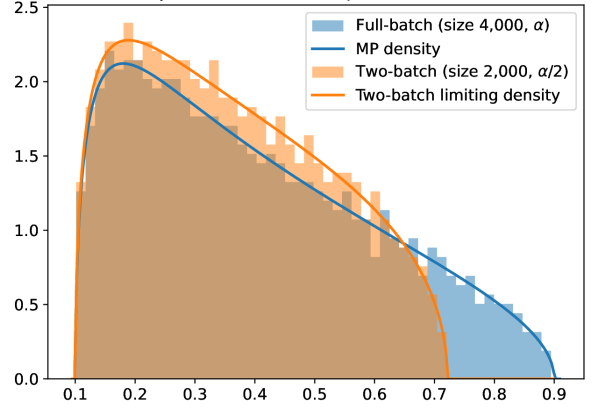
(a) Underparameterized case with $\gamma=1/4$ ($n=4,000$, $p=1,000$), and $\alpha=0.4$.

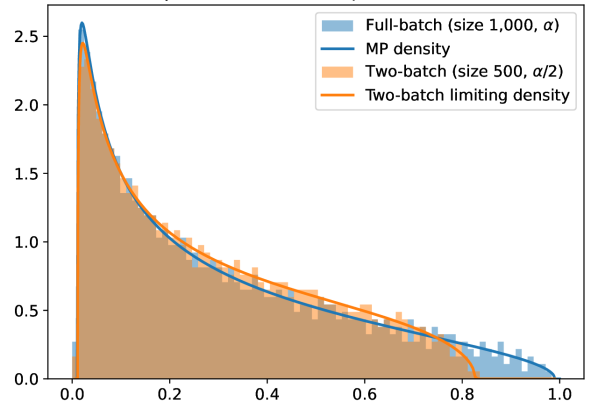
(b) Overparameterized case with $\gamma=3/2$ ($n=1,000$, $p=1,500$), and $\alpha=0.2$. Each distribution has a point mass of $(1-\gamma)^{-1}$ at zero not shown.

Figure 6.1: Comparison of the theoretical limiting spectral distributions of $\alpha\mathbf{W}$ and $\alpha\mathbf{Z}(\alpha/2)$ (lines) with spectral distributions from simulated $n\times p$ standard Gaussian matrices (histograms).

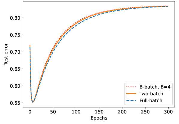
(a) Entire trajectory over 300 epochs.

(b) Limiting trajectory in the last 50 epochs.

Figure 6.2: Empirical generalization error dynamics with $1,000\times 1,500$ standard Gaussian data ($\gamma=3/2$), $\sigma=0.5$, and $\bm{\beta}_{*}$ sampled uniformly at random from the unit sphere. Gradient descent with step size $\alpha=0.2$ compared to $B$-batch gradient descent with step size $\alpha/B$ for $B=2,4$. The test error is averaged over $1,000$ simulations with $1,000$ test samples in each.

In Figure 6.1, we compute the limiting spectral distributions of $\alpha\mathbf{Z}(\alpha/2)$ and $\alpha\mathbf{W}$ in the underparameterized ($\gamma<1$) and overparameterized ($\gamma>1$) regimes, and compare them with the corresponding empirical spectra from a single simulated $n\times p$ Gaussian matrix $\mathbf{X}$. First, the close adherence between the theoretical predictions and the simulations using moderately-sized matrices highlights the predictive capacity of the asymptotic theory. Next, we see that batching results in a complicated transformation of the spectrum of the sample covariance matrix $\alpha\mathbf{W}$. The largest eigenvalues are consistently pushed in, reflecting a shrinkage in the directions that are learned more quickly. The density of the smaller eigenvalues, which magnify the generalization error from overfitting the noise, is typically higher; however, the peak near the edge closest to zero is less pronounced.

Figure 6.2 shows the generalization error dynamics of full-batch gradient descent with step size $\alpha$ and $B$-batch gradient descent with step size $\alpha/B$ for $B=2,4$ in the overparameterized regime. Overall, the difference is slight, highlighting how the full-batch and mini-batch dynamics are matched using the linear scaling rule. However, the difference is visually apparent during the middle of training, and we found that the limiting risks do differ by a tiny amount (with the mini-batch limits being larger by $\sim 0.01$). For an extreme illustration of the differences that can be caused by step size effects, $\alpha$ can be taken to be slightly larger than $n^{-1}\lVert\mathbf{X}^{{\mkern-1.5mu\mathsf{T}}}\mathbf{X}\rVert\sim(1+\sqrt{\gamma})^{2}$ (by the Bai-Yin law [BS10]); in this case, full-batch gradient descent typically diverges, but two-batch gradient descent still converges. See Appendix LABEL:app:numerical_exp for a demonstration and additional numerical experiments.

7 Conclusion

We showed that the error dynamics of a model of mini-batch gradient descent for least squares regression where the mini-batches are sampled without replacement depend on a sample cross-covariance matrix $\mathbf{Z}$ between the original features and a set of new features that have been modified by the other mini-batches. Using this connection, we rigorously established that the linear scaling rule for the step size matches the dynamics of mini-batch and full-batch gradient descent up to leading order with respect to the step size. Finally, we used tools from free probability theory to numerically investigate the effects of batching on the spectrum of $\mathbf{Z}$.

Appendices

The organization of the appendices is as follows:

• Appendix A contains the technical proofs for the results for full-batch gradient descent (Appendix A.1), mini-batch gradient descent (Appendix A.2), and two-batch gradient descent (Appendix LABEL:app:twobatch_gd).

• Appendix LABEL:app:freeprob_alg provides a high-level overview and details on our implementation of the algorithm from [BMS17] for calculating the spectral distribution of a polynomial of free random variables.

• Appendix LABEL:app:numerical_exp presents some additional numerical experiments.

Appendix A Technical proofs

A.1 Full-batch gradient descent

Proof of Lemma 3.1.

Since $\mathbf{y}=\mathbf{X}\bm{\beta}_{*}+\bm{\eta}$, the error vector satisfies the recursive relationship

$$\bm{\beta}_{k}-\bm{\beta}_{*}=\left(\mathbf{I}-\frac{\alpha}{n}\mathbf{X}^{{\mkern-1.5mu\mathsf{T}}}\mathbf{X}\right)(\bm{\beta}_{k-1}-\bm{\beta}_{*})+\frac{\alpha}{n}\mathbf{X}^{{\mkern-1.5mu\mathsf{T}}}\bm{\eta}.$$

By recursively applying this relationship, and instating the definition of $\mathbf{W}=\frac{1}{n}\mathbf{X}^{{\mkern-1.5mu\mathsf{T}}}\mathbf{X}$, we obtain

$$\bm{\beta}_{k}-\bm{\beta}_{*}=\left(\mathbf{I}-\alpha\mathbf{W}\right)^{k}(\bm{\beta}_{0}-\bm{\beta}_{*})+\frac{\alpha}{n}\sum_{j=1}^{k}\left(\mathbf{I}-\alpha\mathbf{W}\right)^{k-j}\mathbf{X}^{{\mkern-1.5mu\mathsf{T}}}\bm{\eta}.$$

The proof of (3.1) is completed by using the following identity to simplify the expression for the sum above, which follows from considering the eigendecomposition of the symmetric matrix $\mathbf{X}$:

$$\sum_{j=1}^{k}\left(\mathbf{I}-\alpha\mathbf{W}\right)^{k-j}\mathbf{X}^{{\mkern-1.5mu\mathsf{T}}}=\left[\mathbf{I}-\left(\mathbf{I}-\alpha\mathbf{W}\right)^{k}\right]\left(\alpha\mathbf{W}\right)^{\dagger}\mathbf{X}^{{\mkern-1.5mu\mathsf{T}}}.$$

Finally, by incorporating the decomposition of the initial error

$$\bm{\beta}_{0}-\bm{\beta}_{*}=\mathbf{P}_{0}(\bm{\beta}_{0}-\bm{\beta}_{*})+\mathbf{P}(\bm{\beta}_{0}-\bm{\beta}_{*}),$$

noting that $(\mathbf{I}-\alpha\mathbf{W})^{k}\mathbf{P}_{0}=\mathbf{P}_{0}$, we obtain (3.2). ∎

Proof of Lemma 3.2.

Note that $\lVert\bm{\beta}_{k}-\bm{\beta}_{*}\rVert^{2}_{\Sigma}=\lVert\Sigma^{1/2}(\bm{\beta}_{k}-\bm{\beta}_{*})\rVert^{2}_{2}$, where $\lVert\cdot\rVert_{2}$ is the usual $\ell_{2}$ norm. Hence, we may expand the square in (3.1) of Lemma 3.1, and use the fact that the cross-terms with a linear dependence on the mean-zero noise term $\bm{\eta}$ vanish upon taking expectation. The first term of this expansion, combined with the decomposition of the initial error in (3.2), yields the first two terms of the claimed generalization error, corresponding to the bias. The remaining variance term follows from writing the second term of the expansion as a trace (i.e. writing $\lVert\mathbf{z}^{{\mkern-1.5mu\mathsf{T}}}\mathbf{z}\rVert_{2}^{2}=\operatorname{Tr}\left(\mathbf{z}\mathbf{z}^{{\mkern-1.5mu\mathsf{T}}}\right)$), using the fact that $\mathbb{E}\left[\bm{\eta}\bm{\eta}^{{\mkern-1.5mu\mathsf{T}}}\right]=\sigma^{2}\,\mathbf{I}$, the cyclic property of trace, and the property $\mathbf{W}^{\dagger}\mathbf{W}\mathbf{W}^{\dagger}=\mathbf{W}^{\dagger}$ of the pseudoinverse. ∎

A.2 Mini-batch gradient descent

A.2.1 Proof of Lemma 4.1

Since $\mathbf{Z}=\frac{1}{n}\widetilde{\mathbf{X}}^{{\mkern-1.5mu\mathsf{T}}}\mathbf{X}=\frac{1}{n}\sum_{b=1}^{B}\widetilde{\mathbf{X}}_{b}^{{\mkern-1.5mu\mathsf{T}}}\mathbf{X}_{b}=\frac{1}{n}\sum_{b=1}^{B}\Pi_{b}\mathbf{X}_{b}^{{\mkern-1.5mu\mathsf{T}}}\mathbf{X}_{b}$, it suffices to show that

$$\sum_{b=1}^{B}\Pi_{b}\mathbf{W}_{b}=\sum_{b=1}^{B}\mathbf{W}_{b}\Pi_{b}$$

to prove that $\mathbf{Z}$ is symmetric. Fix $b\in\{1,\dots,B\}$. Note that $\Pi_{b}\mathbf{W}_{b}$ and $\mathbf{W}_{b}\Pi_{b}$ are polynomials in the non-commuting variables $\mathbf{W}_{1},\dots,\mathbf{W}_{B}$, and that $\Pi_{b}$ does not contain the term $\mathbf{W}_{b}$. Hence, it suffices to argue that the word ending in $\mathbf{W}_{b}$ on the left hand side – i.e. $\Pi_{b}\mathbf{W}_{b}$ – matches the word ending in $\mathbf{W}_{b}$ on the right hand side – i.e. the sum of the words ending in $\mathbf{W}_{b}$ in $\sum_{j\neq b}\mathbf{W}_{j}\Pi_{j}$.

Observe that $\Pi_{b}\mathbf{W}_{b}$ is a sum of words of the form $a_{i_{1},\dots,i_{\ell}}\mathbf{W}_{i_{1}}\mathbf{W}_{i_{2}}\cdots\mathbf{W}_{i_{\ell}}\mathbf{W}_{b}$, where each of the indices are distinct and $a_{i_{1},\dots,i_{\ell}}\in\mathbb{R}$ is a constant. From the form of $\Pi_{b}$, this term arises as a sum over permutations $\tau$ from a set, say $\mathcal{T}\equiv\mathcal{T}_{i_{1},\dots,i_{\ell}}$, such that $\tau(i_{\ell})<\dots<\tau(i_{2})<\tau(i_{1})<\tau(b)$:

$$a_{i_{1},\dots,i_{\ell}}\mathbf{W}_{i_{1}}\mathbf{W}_{i_{2}}\cdots\mathbf{W}_{i_{\ell}}\mathbf{W}_{b}=\left(\frac{1}{B!}\sum_{\tau\in\mathcal{T}}(-\alpha)^{\ell}\mathbf{W}_{i_{1}}\mathbf{W}_{i_{2}}\cdots\mathbf{W}_{i_{\ell}}\right)\mathbf{W}_{b}.$$

The same word arises in the expression $\sum_{j\neq b}\mathbf{W}_{j}\Pi_{j}$ from the single term $\mathbf{W}_{i_{1}}\Pi_{i_{1}}$ with $\mathbf{W}_{i_{1}}$ as the leftmost matrix in the product. For each $\tau\in\mathcal{T}$, consider shifting the sub-permutation $(i_{1},i_{2},\dots,i_{\ell},b)$ in $\tau$ cyclically to the right (keeping the other entries fixed) to obtain the permutation $\tau^{\prime}$ with sub-permutation $(b,i_{1},i_{2},\dots,i_{\ell})$. If $\mathcal{T}^{\prime}$ denotes the set of permutations obtained from $\mathcal{T}$ in this way, then by summing over all $\tau^{\prime}\in\mathcal{T}$ in $\Pi_{i_{1}}$ – choosing the term $-\alpha\mathbf{W}_{\tau^{\prime}(j)}$ for each $j\in\{i_{2},\dots,i_{\ell},b\}$, and $\mathbf{I}$ for the rest of the indices in the product over $\tau^{\prime}$ – this shows that the word $a^{\prime}_{i_{2},\dots,i_{\ell},b}\mathbf{W}_{i_{1}}\mathbf{W}_{i_{2}}\cdots\mathbf{W}_{i_{\ell}}\mathbf{W}_{b}$ appearing in $\mathbf{W}_{i_{1}}\Pi_{i_{1}}$ is equal to

$$\mathbf{W}_{i_{1}}\left(\frac{1}{B!}\sum_{\tau^{\prime}\in\mathcal{T}^{\prime}}(-\alpha)^{\ell}\mathbf{W}_{i_{2}}\cdots\mathbf{W}_{i_{\ell}}\mathbf{W}_{b}\right)=a_{i_{1},\dots,i_{\ell}}\mathbf{W}_{i_{1}}\mathbf{W}_{i_{2}}\cdots\mathbf{W}_{i_{\ell}}\mathbf{W}_{b}.$$

Thus, we conclude that $\sum_{b=1}^{B}\Pi_{b}\mathbf{W}_{b}=\sum_{b=1}^{B}\mathbf{W}_{b}\Pi_{b}$, and hence $\mathbf{Z}$ is symmetric.

Next, we will prove that $.Inthefollowing,let$$\mathbf{w}$∈R^n$beagenericvectorpartitionedinto$$\mathbf{w}$_1, …, $\mathbf{w}$_B$inthesamewayasthebatches$$\mathbf{X}$_1, …, $\mathbf{X}$_b$.Since$$\mathbf{Z}$$issymmetric,$$\mathbf{Z}$^T $\mathbf{w}$= 1n ∑_b=1^B ~$\mathbf{X}$_b^T $\mathbf{X}$_b $\mathbf{w}$= 1n ∑_b=1^B $\mathbf{X}$_b^T ~$\mathbf{X}$_b $\mathbf{w}$$,andhenceitisclearthattherowspaceof$$\mathbf{Z}$$iscontainedintherowspaceof$~$\mathbf{X}$$.Furthermore,fromexpandingtheproductin$Π_b$,wecanwrite$~$\mathbf{X}$^T $\mathbf{w}$= ∑_b=1^B Π_b $\mathbf{X}$_b^T $\mathbf{w}$_b = ∑_b=1^B $\mathbf{X}$_b^T $\mathbf{w}$_b + ∑_b=1^B α_b $\mathbf{X}$_b^T $\mathbf{X}$_b v_b$forsomecoefficients$α_b ∈R$andvectors$v_b$.Hence,therowspaceof$~$\mathbf{X}$$iscontainedintherowspaceofof$$\mathbf{X}$$.\qed\par\par$

A.2.2 Proof of Theorem 4.3

Lemma A.1.

Let $\mathbf{A}\in\mathbb{R}^{p\times p}$ be a symmetric matrix, and define $\mathbf{P}=(\mathbf{I}-\mathbf{A})(\mathbf{I}-\mathbf{A})^{\dagger}$ and $\mathbf{P}_{0}=\mathbf{I}-\mathbf{P}$ to be the orthogonal projectors onto the range and kernel of $\mathbf{I}-\mathbf{A}$ respectively. Then we have

$$(\mathbf{I}+\mathbf{A}+\dots+\mathbf{A}^{k-1})=(\mathbf{I}-\mathbf{A}^{k})(\mathbf{I}-\mathbf{A})^{\dagger}+k\mathbf{P}_{0}.$$

Proof.

Since $\mathbf{I}=\mathbf{P}+\mathbf{P}_{0}$, we can write $(\mathbf{I}+\mathbf{A}+\dots+\mathbf{A}^{k-1})=(\mathbf{I}+\mathbf{A}+\dots+\mathbf{A}^{k-1})(\mathbf{P}+\mathbf{P}_{0})$. By multiplying both sides of the algebraic identity $(\mathbf{I}+\mathbf{A}+\dots+\mathbf{A}^{k-1})(\mathbf{I}-\mathbf{A})=(\mathbf{I}-\mathbf{A}^{k})$ by $(\mathbf{I}-\mathbf{A})^{\dagger}$, we have $(\mathbf{I}+\mathbf{A}+\dots+\mathbf{A}^{k-1})\mathbf{P}=(\mathbf{I}-\mathbf{A}^{k})(\mathbf{I}-\mathbf{A})^{\dagger}$, which yields the first term. For the second term, note that $\mathbf{A}^{\ell}\mathbf{P}_{0}=\mathbf{P}_{0}$ for any $\ell\geq 1$, since $\mathbf{A}\mathbf{x}=\mathbf{x}$ for any $\mathbf{x}$ in the kernel of $\mathbf{I}-\mathbf{A}$. Thus, $(\mathbf{I}+\mathbf{A}+\dots+\mathbf{A}^{k-1})\mathbf{P}_{0}=k\mathbf{P}_{0}$, which yields the second term. ∎

Proof of Theorem 4.3.

Recall that from (2.2), the iterates $\bm{\beta}_{k}^{(b)}$ from mini-batch gradient descent after $b$ iterations over the mini-batches in the $k$th epoch satisfy

$$\bm{\beta}_{k}^{(b)}=\bm{\beta}_{k}^{(b)}-\frac{B\alpha}{n}\mathbf{X}_{\tau(b)}^{{\mkern-1.5mu\mathsf{T}}}(\mathbf{X}_{\tau(b)}\bm{\beta}_{k}^{(b-1)}-\mathbf{y}_{\tau(b)}),\quad b=1,2,\dots,B,$$

given a permutation $\tau=(\tau(1),\tau(2),\dots,\tau(B))$ of the mini-batches in the $k$th epoch, where $\bm{\beta}_{k}^{(0)}:=\bm{\beta}_{k-1}^{(B)}$ and $\bm{\beta}_{0}^{(B)}:=\bm{\beta}_{0}$. By using the fact that $\mathbf{y}_{b}=\mathbf{X}_{b}\bm{\beta}_{*}+\bm{\eta}_{b}$ for each mini-batch, the displayed equation above rearranges to

$$\bm{\beta}_{k}^{(b)}-\bm{\beta}_{*}=\left(\mathbf{I}-\frac{B\alpha}{n}\mathbf{X}_{\tau(b)}^{{\mkern-1.5mu\mathsf{T}}}\mathbf{X}_{\tau(b)}\right)(\bm{\beta}_{k}^{(b-1)}-\bm{\beta}_{*})+\frac{B\alpha}{n}\mathbf{X}_{\tau(b)}^{{\mkern-1.5mu\mathsf{T}}}\bm{\eta}_{\tau(b)},\quad b=1,2,\dots,B.$$

By iterating this relationship, we deduce that the estimate at the end of the $k$th epoch satisfies

$$\bm{\beta}_{k}^{(B)}-\bm{\beta}_{*}=\prod_{b=1}^{B}(\mathbf{I}-\alpha\mathbf{W}_{\tau(b)})(\bm{\beta}_{k-1}^{(B)}-\bm{\beta}_{*})+\frac{B\alpha}{n}\sum_{b=1}^{B}\prod_{j:\tau(j)<\tau(b)}(\mathbf{I}-\alpha\mathbf{W}_{\tau(j)})\mathbf{X}_{b}^{{\mkern-1.5mu\mathsf{T}}}\bm{\eta}_{b}.$$ (A.1)

Recall that $\bar{\bm{\beta}}_{k}=\mathbb{E}_{\tau\sim\mathrm{Unif}(S_{B})}\left[\bm{\beta}_{k}^{(B)}\right]$. Hence, by taking the expectation over the random permutations of the batches in each epoch, drawn uniformly from the $B!$ permutations in the symmetric group $S_{B}$ of $B$ elements, the error vector $\bar{\bm{\beta}}_{k}-\bm{\beta}_{*}$ satisfies the recursive relationship

$$\bar{\bm{\beta}}_{k}-\bm{\beta}_{*} =\frac{1}{B!}\sum_{\tau\in S_{B}}\prod_{b=1}^{B}(\mathbf{I}-\alpha\mathbf{W}_{\tau(b)})(\bar{\bm{\beta}}_{k-1}-\bm{\beta}_{*})$$ (A.2)

$$\quad+\frac{B\alpha}{n}\left\{\frac{1}{B!}\sum_{\tau\in S_{B}}\sum_{b=1}^{B}\prod_{j:\tau(j)<\tau(b)}(\mathbf{I}-\alpha\mathbf{W}_{\tau(j)})\mathbf{X}_{b}^{{\mkern-1.5mu\mathsf{T}}}\right\}\bm{\eta}_{b}.$$

By moving the sum over $b$ outside, the second term is equal to

$$\frac{B\alpha}{n}\sum_{b=1}^{B}\widetilde{\mathbf{X}}_{b}^{{\mkern-1.5mu\mathsf{T}}}\bm{\eta}_{b}=\frac{B\alpha}{n}\widetilde{\mathbf{X}}^{{\mkern-1.5mu\mathsf{T}}}\bm{\eta},$$

simply by definition of the modified features $\widetilde{\mathbf{X}}_{b}$ from (4.1). Next, by writing $\mathbf{Z}=\frac{1}{n}\sum_{b=1}^{B}\widetilde{\mathbf{X}}_{b}^{{\mkern-1.5mu\mathsf{T}}}\mathbf{X}_{b}$, we have

$$\mathbf{Z}=\frac{1}{B\alpha}\left(\frac{1}{B!}\sum_{\tau\in S_{B}}\sum_{b=1}^{B}\prod_{j:\tau(j)<\tau(b)}(\mathbf{I}-\alpha\mathbf{W}_{\tau(j)})\alpha\mathbf{W}_{b}\right).$$ (A.3)

We claim that the identity

$$\frac{1}{B!}\sum_{\tau\in S_{B}}\sum_{b=1}^{B}\prod_{j:\tau(j)<\tau(b)}(\mathbf{I}-\alpha\mathbf{W}_{\tau(j)})\alpha\mathbf{W}_{b}=\mathbf{I}-\frac{1}{B!}\sum_{\tau\in S_{B}}\prod_{b=1}^{B}(\mathbf{I}-\alpha\mathbf{W}_{\tau(b)})$$ (A.4)

holds. Assuming that this is true for now, combining (A.3) and (A.4) shows that (A.2) can be written as

$$\bar{\bm{\beta}}_{k}-\bm{\beta}_{*}=(\mathbf{I}-B\alpha\mathbf{Z})(\bar{\bm{\beta}}_{k-1}-\bm{\beta}_{*})+\frac{B\alpha}{n}\widetilde{\mathbf{X}}^{{\mkern-1.5mu\mathsf{T}}}\bm{\eta}.$$ (A.5)

Hence, by recursively applying this relationship, we obtain

$$\bar{\bm{\beta}}_{k}-\bm{\beta}_{*}=(\mathbf{I}-B\alpha\mathbf{Z})^{k}(\bm{\beta}_{0}-\bm{\beta}_{*})+\frac{B\alpha}{n}\sum_{j=1}^{k}(\mathbf{I}-B\alpha\mathbf{Z})^{k-j}\widetilde{\mathbf{X}}^{{\mkern-1.5mu\mathsf{T}}}\bm{\eta}.$$

The proof of (4.5) is completed by using the following identity from Lemma A.1 to simplify the expression for the sum above. Here, we use the assumption that $todeducethat$$\mathbf{P}$_$\mathbf{Z}$, 0 ~$\mathbf{X}$^T = 0$(i.e.\$$\mathbf{Z}$~$\mathbf{X}$^T $\bm{\eta}$= 0$ifandonlyif$

References

- [ASS20] Madhu S. Advani, Andrew M. Saxe and Haim Sompolinsky “High-dimensional dynamics of generalization error in neural networks” In Neural Networks 132, 2020, pp. 428–446 DOI: 10.1016/j.neunet.2020.08.022
- [AKT19] Alnur Ali, J. Kolter and Ryan J. Tibshirani “A Continuous-Time View of Early Stopping for Least Squares Regression” In International Conference on Artificial Intelligence and Statistics (AISTATS), 2019, pp. 1370–1378 arXiv:1810.10082 [stat.ML]
- [Ari+24] Octavio Arizmendi, Guillaume Cébron, Roland Speicher and Sheng Yin “Universality of free random variables: Atoms for non-commutative rational functions” In Advances in Mathematics 443, 2024, pp. 109595 DOI: 10.1016/j.aim.2024.109595
- [Ba+22] Jimmy Ba, Murat A. Erdogdu, Taiji Suzuki, Zhichao Wang, Denny Wu and Greg Yang “High-dimensional Asymptotics of Feature Learning: How One Gradient Step Improves the Representation” In Advances in Neural Information Processing Systems, 2022 arXiv:2205.01445 [stat.ML]
- [BS10] Zhidong Bai and Jack W. Silverstein “Spectral Analysis of Large Dimensional Random Matrices” Springer New York, NY, 2010 DOI: 10.1007/978-1-4419-0661-8
- [BMS17] Serban T. Belinschi, Tobias Mai and Roland Speicher “Analytic subordination theory of operator-valued free additive convolution and the solution of a general random matrix problem” In Journal für die reine und angewandte Mathematik 2017.732, 2017, pp. 21–53 DOI: 10.1515/crelle-2014-0138
- [Bot09] Léon Bottou “Curiously fast convergence of some stochastic gradient descent algorithms” Unpublished open problem offered to the attendance of the SLDS 2009 conference, 2009
- [Bot12] Léon Bottou “Stochastic Gradient Descent Tricks” In Neural Networks: Tricks of the Trade Springer Berlin Heidelberg, 2012, pp. 421–436 DOI: 10.1007/978-3-642-35289-8_25
- [COB19] Lénaı̈c Chizat, Edouard Oyallon and Francis Bach “On Lazy Training in Differentiable Programming” In Advances in Neural Information Processing Systems 32, 2019 arXiv:1812.07956 [math.OC]
- [CL22] Romain Couillet and Zhenyu Liao “Random Matrix Methods for Machine Learning” Cambridge University Press, 2022 DOI: 10.1017/9781009128490
- [Dob18] Dobriban, Edgar and Wager, Stefan “High-dimensional asymptotics of prediction: Ridge regression and classification” In The Annals of Statistics 46.1, 2018, pp. 247–279 DOI: 10.1214/17-AOS1549
- [Du+19] Simon Du, Jason Lee, Haochuan Li, Liwei Wang and Xiyu Zhai “Gradient Descent Finds Global Minima of Deep Neural Networks” In International Conference on Machine Learning 97, 2019, pp. 1675–1685 arXiv:1811.03804 [cs.LG]
- [Du+19a] Simon S. Du, Xiyu Zhai, Barnabas Poczos and Aarti Singh “Gradient Descent Provably Optimizes Over-parameterized Neural Networks” In International Conference on Learning Representations, 2019 arXiv:1810.02054 [cs.LG]
- [Gei+22] Jonas Geiping, Micah Goldblum, Phil Pope, Michael Moeller and Tom Goldstein “Stochastic Training is Not Necessary for Generalization” In International Conference on Learning Representations, 2022 arXiv:2109.14119 [cs.LG]
- [Gow+19] Robert Mansel Gower, Nicolas Loizou, Xun Qian, Alibek Sailanbayev, Egor Shulgin and Peter Richtárik “SGD: General Analysis and Improved Rates” In International Conference on Machine Learning 97, 2019, pp. 5200–5209 arXiv:1901.09401 [cs.LG]
- [Goy+18] Priya Goyal et al. “Accurate, Large Minibatch SGD: Training ImageNet in 1 Hour” Technical report, arXiv:1706.02677, 2018 arXiv:1706.02677 [cs.CV]
- [GZR22] Diego Granziol, Stefan Zohren and Stephen Roberts “Learning Rates as a Function of Batch Size: A Random Matrix Theory Approach to Neural Network Training” In Journal of Machine Learning Research 23.173, 2022, pp. 1–65 arXiv:2006.09092 [stat.ML]
- [Gun+18] Suriya Gunasekar, Jason Lee, Daniel Soudry and Nathan Srebro “Characterizing Implicit Bias in Terms of Optimization Geometry” In International Conference on Machine Learning 80, 2018, pp. 1832–1841 arXiv:1802.08246 [stat.ML]
- [Gun+18a] Suriya Gunasekar, Jason D. Lee, Daniel Soudry and Nati Srebro “Implicit Bias of Gradient Descent on Linear Convolutional Networks” In Advances in Neural Information Processing Systems 31, 2018 arXiv:1806.00468 [cs.LG]
- [Gür21] Gürbüzbalaban, Mert and Ozdaglar, Asuman and Parrilo, Pablo A. “Why random reshuffling beats stochastic gradient descent” In Mathematical Programming 186, 2021, pp. 49–84 DOI: 10.1007/s10107-019-01440-w
- [Has+22] Trevor Hastie, Andrea Montanari, Saharon Rosset and Ryan J. Tibshirani “Surprises in high-dimensional ridgeless least squares interpolation” In The Annals of Statistics 50.2, 2022, pp. 949–986 DOI: 10.1214/21-AOS2133
- [HLT19] Fengxiang He, Tongliang Liu and Dacheng Tao “Control Batch Size and Learning Rate to Generalize Well: Theoretical and Empirical Evidence” In Advances in Neural Information Processing Systems 32, 2019
- [KSS24] Chinmaya Kausik, Kashvi Srivastava and Rishi Sonthalia “Double Descent and Overfitting under Noisy Inputs and Distribution Shift for Linear Denoisers” In Transactions on Machine Learning Research, 2024 arXiv:2305.17297 [cs.LG]
- [Kri14] Alex Krizhevsky “One weird trick for parallelizing convolutional neural networks” "preprint, arXiv:1404.5997", 2014 arXiv:1404.5997 [cs.NE]
- [Mal+22] Sadhika Malladi, Kaifeng Lyu, Abhishek Panigrahi and Sanjeev Arora “On the SDEs and Scaling Rules for Adaptive Gradient Algorithms” In Advances in Neural Information Processing Systems, 2022 arXiv:2205.10287 [cs.LG]
- [Mar67] Marčenko, Vladimir A. and Pastur, Leonid Andreevich “Distribution of eigenvalues for some sets of random matrices” In Mathematics of the USSR-Sbornik 1.4, 1967, pp. 457 DOI: 10.1070/SM1967v001n04ABEH001994
- [Mei22] Mei, Song and Montanari, Andrea “The Generalization Error of Random Features Regression: Precise Asymptotics and the Double Descent Curve” In Communications on Pure and Applied Mathematics 75, 2022, pp. 667–766 DOI: 10.1002/cpa.22008
- [MS17] James A. Mingo and Roland Speicher “Free Probability and Random Matrices” Springer New York, NY, 2017 DOI: 10.1007/978-1-4939-6942-5
- [MM23] Theodor Misiakiewicz and Andrea Montanari “Six Lectures on Linearized Neural Networks” preprint, arXiv:2308.13431, 2023 arXiv:2308.13431 [stat.ML]
- [Paq+22] Courtney Paquette, Elliot Paquette, Ben Adlam and Jeffrey Pennington “Implicit Regularization or Implicit Conditioning? Exact Risk Trajectories of SGD in High Dimensions” In Advances in Neural Information Processing Systems 35, 2022, pp. 35984–35999 arXiv:2206.07252 [stat.ML]
- [RE08] N. Raj Rao and Alan Edelman “The Polynomial Method for Random Matrices” In Foundations of Computational Mathematics 8, 2008, pp. 649–702 DOI: 10.1007/s10208-007-9013-x
- [RDR22] Dominic Richards, Edgar Dobriban and Patrick Rebeschini “Comparing Classes of Estimators: When does Gradient Descent Beat Ridge Regression in Linear Models?” preprint, arXiv:2108.11872, 2022 arXiv:2108.11872 [math.ST]
- [SGB94] K. Skouras, C. Goutis and M.J. Bramson “Estimation in linear models using gradient descent with early stopping” In Statistics and Computing 4, 1994, pp. 271–278 DOI: 10.1007/BF00156750
- [Smi+18] Samuel L. Smith, Pieter-Jan Kindermans, Chris Ying and Quoc V. Le “Don’t Decay the Learning Rate, Increase the Batch Size” In International Conference on Learning Representations, 2018 arXiv:1711.00489 [cs.LG]
- [WSH24] Yutong Wang, Rishi Sonthalia and Wei Hu “Near-interpolators: Rapid norm growth and the trade-off between interpolation and generalization” In International Conference on Artificial Intelligence and Statistics, 2024, pp. 4483–4491 arXiv:2403.07264 [cs.LG]