Dynamical phase transitions in two-dimensional Brownian Matter

Abstract

We investigate a system of two-dimensional interacting Brownian particles at finite density. In the continuum limit, we uncover a hidden symmetry under area-preserving diffeomorphism transformations. This symmetry leads to the conservation of local vorticity. By calculating the generating functional within the saddle-point plus Gaussian fluctuations approximation, we reveal the emergence of a $U(1)$ gauge symmetry. This emergent symmetry enables us to describe the dynamics of density fluctuations as a gauge theory. We solve the corresponding equations of motion for various local and non-local two-body potentials, demonstrating the presence of multiple dynamical regimes and associated dynamical phase transitions.

I Introduction

The study of Brownian matter, i.e., a huge number of interacting Brownian particles, offers a rich variety of phenomena to explore. It provides valuable insights into universal principles of statistical physics, such as the role of fluctuations and the importance of symmetry breaking in driving phase transitions[1].

One of the most intriguing aspects of collective phenomema is pattern formation, where seemingly disordered systems give rise to structured arrangements and spatial organization. From the spontaneous formation of intricate fractal patterns to the emergence of self-assembled structures with remarkable complexity [2], the realm of Brownian matter is a playground for understanding the principles governing pattern formation in nature.

Beyond its theoretical significance, the study of Brownian matter holds practical implications in diverse fields. In materials science, insights into the self-assembly of colloidal particles[3, 4] offer pathways for designing novel materials with tailored properties, ranging from advanced ceramics to functional coatings. In biophysics, understanding the dynamics of biomolecules in cellular environments sheds light on crucial processes like protein folding and intracellular transport[5].

From the technical point of view, besides numerical simulations, the mathematical methods to address these types of systems prove to be quite intricate. The hydrodynamic limit is usually taken using the Dean-Kawasaki[6, 7] equation. The main idea behind this method is to describe the evolution of the density of particles by means of a closed functional Langevin equation [8].

In this work, we follow and alternative road. By means of the Martin-Siggia-Rose-Jenssen-De Dominicis (MSRJD) formalism[9, 10, 11] , we built a generating functional for correlation functions, subsequently considering the transition to the continuum limit. In this limit, we show a hidden symmetry generated by area preserving diffeomorphisms transformations. The physical consequence of this symmetry is the conservation of the local vorticity making contact with the Kelvin circulation theorem of fluid mechanics[12].

In the weak density fluctuations limit, this symmetry emerges as a simple $U(1)$ gauge symmetry, providing an effective dual gauge theory for the dynamics of density fluctuations. In a previous paper[13], we apply this method to a system of active particles, focusing in the orientational degrees of freedom. Here, we explore the consequence of these symmetries in a passive system for different types of microscopic interactions. In particular, we focus in the dynamical regime, showing the conditions for the appearance of dynamical phase transitions.

The main result of this paper is the dual gauge theory represented by the effective action of equation (49). The emergent “magnetic field” represents weak density flucutations around an homogeneous background, while the emergent electric field keep track of the conservation of local vorticity that, in the effective theory, emerges as “charge” conservation. The non-local “magnetic susceptibility” is determined by microscopic two-body interactions.

We have studied both, local as well as non-local two-body potentials. In the local repulsive case, we show that a static homogeneous density is stable, since weak fluctuations are damped to zero. However, in the attractive case, the combination of interaction and thermal fluctuations induces a critical temperature above which the Brownian system behaves as a dispersive medium where sound waves can be propagated. We have also studied purely repulsive non-local potentials, such as the two-dimensional dipolar and a class of soft core interactions. In both cases we show the appearance of dynamical phase transitions separating dissipative and a dispersive phases. At the transition regions, static pattern formation is possible. However, the non-analiticity of the dispersion relation suggest that the transitions do not correspond with the usual Brazovskii-Swift-Hohembergh mechanism[14, 15].

The paper is structured as follows: In section II we introduce the model and the formalism. In section III we present the central result of the paper, i.e., we show the appearance of an emergent gauge symmetry and build up the effective action for density fluctuations. We study the dynamic of density fluctuations in section IV and show, in section V and VI, some results on dynamical phase transitions for particular microscopic two-body interactions. In section VII, we present our conclusions leaving some mathematical details of the calculation for appendix A.

II Interacting two-dimensional Brownian particles

The simplest model for $N$ two-dimensional interacting Brownian particles is given by a system of overdamped Langevin equations,

$$\frac{d{\bf r}_{i}(t)}{dt} =-\sum_{j\neq i}\bm{\nabla}U(|{\bf r}_{i}-{\bf r}_{j}|))+\bm{\xi}^{T}_{i}(t)\;,$$ (1)

with white noise,

$$\langle\xi^{T}_{\alpha,i}\rangle =0$$ (2)

$$\langle\xi^{T}_{i,\alpha}(t)\xi^{T}_{j,\beta}(t^{\prime})\rangle =2k_{B}T\delta_{ij}\delta_{\alpha\beta}\delta(t-t^{\prime})\;.$$ (3)

${\bf r}_{i}(t)$ with $i=1,\ldots,N$ are the two-dimensional position vectors of each particle as a function of time. In these equations, Latin indexes $i,j=1,\ldots,N$ label the particles, while the Greek indexes $\alpha,\beta=1,2$ are Cartesian components in the plane $r_{\alpha}\equiv\{x_{1},x_{2}\}$. $U(|{\bf r}_{i}-{\bf r}_{j}|))$ is a pair potential between particles and $k_{B}T$ is the thermal energy of the bath ($k_{B}$ is the Boltzmann constant). Along the paper, we use bold characters for vector quantities.

We are interested in studding symmetries and collective behavior of this system. For this, a functional formalism is an appropriate tool.

II.1 Functional formalism

We use the Martin-Siggia-Rose-Jennsen-de Dominicis (MSRJD) formalism to buit up a generating functional of correlation functions. In appendix A we describe the formalism in detail. The generating functional can be cast in the form,

$$Z[\bm{\eta}]= \int\left(\prod_{i}{\cal D}{\bf r}_{i}(t)\right)$$ (4)

$$\times\exp\left\{-\frac{1}{2k_{B}T}S[{\bf r}_{i}]+\sum_{i}\int dt\;\bm{\eta}_{i}\cdot{\bf r}_{i}\right\}$$

where, as before, $i=1,\ldots,N$ labels each particle. The action is given by (please see appendix A)

$$S= \int dt\sum_{i}$$ (5)

$$\times\left\{\frac{1}{2}\left|\frac{d{\bf r}_{i}(t)}{dt}\right|^{2}+\frac{1}{2}\left|\bm{\nabla}_{r_{i}}\tilde{U}\right|^{2}-k_{B}T\nabla_{r_{i}}^{2}\tilde{U}\right\}$$

where

$$\tilde{U}({\bf r}_{i})=\sum_{j\neq i}U(|{\bf r}_{i}-{\bf r}_{j}|)$$ (6)

This formalism is an exact representation of the system of Langevin equations. Once $Z[\bm{\eta}]$ is known, we can compute any correlation function by functional differentiating

$$\left\langle r_{i_{1}}(t_{1})\ldots r_{i_{n}}(t_{n})\right\rangle_{\bm{\xi}}=\left.\frac{\delta^{(n)}Z[\bm{\eta}]}{\delta\eta_{i_{n}}(t_{n})\ldots\delta\eta_{i_{1}}(t_{1})}\right|_{{\bm{\eta}}=0}\;.$$ (7)

III Symmetries

III.1 Continuum limit

Consider a system with a huge number of particles at finite mean density, i. e., the number of particles $N$ per unit area $A$ is finite, even in the limit $N\to\infty,A\to\infty$. Under this assumption, we can take the continuum limit. For this, we simply promote the particle label $i=1,\ldots,N$ to a continuum two-dimensional vector variable ${\bf y}\equiv(y_{1},y_{2})$, in such a way that

$$i \to{\bf y}$$ (8)

$${\bf r}_{i}(t) \to{\bf r}({\bf y},t)\;.$$ (9)

In this way, the set of position vectors ${\bf r}_{i}$ with $i=1,\ldots,N$ turns out to be a two-dimensional vector field ${\bf r}({\bf y},t)$. Moreover, sums over particles turn out to transform into integrals,

$$\sum_{i} \to\rho_{0}\int d^{2}y$$ (10)

where $\rho_{0}$ is a constant density.

The action of Eq. (5) can be written in the continuum limit as

$$S=S_{K}+S_{U}\;,$$ (11)

where the kinetic part is given by

$$S_{K}=\frac{\rho_{0}}{2}\int dtd^{2}y\left|\partial_{t}{\bf r}({\bf y},t)\right|^{2}$$ (12)

and the interaction potential contribution is

$$S_{U} =\frac{\rho_{0}^{3}}{2}\int dtd^{2}yd^{2}y^{\prime}d^{2}y^{\prime\prime}$$

$$\times\bm{\nabla}U({\bf r}({\bf y})-{\bf r}({\bf y}^{\prime}))\cdot\bm{\nabla}U({\bf r}({\bf y})-{\bf r}({\bf y}^{\prime\prime}))$$

$$-k_{B}T\rho_{0}^{2}\int dtd^{2}yd^{2}y^{\prime}\nabla^{2}U({\bf r}({\bf y})-{\bf r}({\bf y}^{\prime}))\;.$$ (13)

In Eqs. (12) and (13), ${\bf r}({\bf y},t)$ is a vector field of $\{{\bf y},t\}$ and $\partial_{t}$ stands for the partial derivative with respect to time.

III.2 Area-preserving diffeomorphisms and vorticity

There is huge freedom in making the transition to the continuum limit. For instance, instead of the variable ${\bf y}$, given by equation (8), we could choose another parametrization ${\bf y}^{\prime}$, as for instance

$$i \to{\bf y}={\bf f}({\bf y}^{\prime})$$ (14)

where ${\bf f}({\bf y})$ is an invertible smooth vector function. Under this transformation, equation (9) transforms as,

$${\bf r}_{i}(t) \to{\bf r}({\bf y},t)={\bf r}({\bf f}({\bf y}^{\prime}),t)\equiv{\bf r}^{\prime}({\bf y}^{\prime})\;.$$ (15)

Therefore, each component of the position vector transforms as a scalar under reparametrizations

$$r^{\prime}_{\alpha}({\bf y}^{\prime})=r_{\alpha}({\bf y})\;.$$ (16)

with $\alpha=1,2$.

Moreover, from equation (10), we find

$$\sum_{i} \to\rho_{0}\int d^{2}y=\rho_{0}\int d^{2}y^{\prime}\det\left(\frac{\partial y_{i}}{\partial y^{\prime}_{j}}\right)$$ (17)

where the $\det\left(\partial y_{i}/\partial y^{\prime}_{j}\right)$ is the Jacobian of the transformation of equation (14).

The action of the system, equation (11) (with the expressions (12) and (13)), is invariant under this reparametrization,

$$S^{\prime}[{\bf r}^{\prime}({\bf y}^{\prime},t)]=S[{\bf r}({\bf y},t)]\;,$$ (18)

provided the Jacobian of the transformation is one, i. e. ,

$$J({\bf y}^{\prime})\equiv\det\left(\frac{\partial y_{i}}{\partial y^{\prime}_{j}}\right)=\det\left(\frac{\partial f_{i}({\bf y}^{\prime})}{\partial y^{\prime}_{j}}\right)=1\;.$$ (19)

In this case, the transformation of Eq. (14) is a mapping between the planes $\{y_{1},y_{2}\}\to\{y^{\prime}_{1},y^{\prime}_{2}\}$ that preserves the area contained in any closed contour. To see this, consider for instance a domain $D\subset\{y_{1},y_{2}\}$ enclosing an area $\Omega$. The transformation of Eq. (14) changes the domain from $D\to D^{\prime}\subset\{y^{\prime}_{1},y^{\prime}_{2}\}$, enclosing a new area $\Omega^{\prime}$. Thus,

$$\Omega=\int_{D}d^{2}y=\int_{D^{\prime}}d^{2}y^{\prime}\;J({\bf y}^{\prime})\;.$$ (20)

In the last equality, we have used equation (14) to transform ${\bf y}\to{\bf y}^{\prime}$ and $D\to D^{\prime}$. Due to the fact that the Jacobian $J({\bf y}^{\prime})=1$ (equation (19)), then, $\Omega^{\prime}=\Omega$.

Therefore, the action $S[{\bf r}({\bf y},t)]$ has an exact symmetry given by its invariance under general area preserving diffeomorphisms (APD).

Noëther theorem associates a conserved quantity with any continuous symmetry of the action. To compute it, it is sufficient to consider only infinitesimal transformations. Explicitly, an infinitesimal APD can be written in the following way,

$$y^{\prime}_{i}=y_{i}+\epsilon_{ij}\frac{\partial\Lambda({\bf y})}{\partial y_{j}}\;,$$ (21)

where $\epsilon_{ij}$ is the completely antisymmetric Levi-Civita tensor and $\Lambda({\bf y})$ is an arbitrary function satisfying

$$\left(\frac{\partial}{\partial y_{1}}\frac{\partial}{\partial y_{2}}-\frac{\partial}{\partial y_{2}}\frac{\partial}{\partial y_{1}}\right)\Lambda({\bf y})=0\;.$$ (22)

It is a simple matter to check from equations (21) and (22), by direct computation, that

$$\det(\frac{\partial y^{\prime}_{i}}{\partial y_{j}})=1+O(\Lambda^{2})\;.$$ (23)

Thus, equation (21) represent an APD at linear order in $\Lambda$.

From equations (16) and (21), the position vector transforms, at linear order in $\Lambda$, as

$$\delta r_{\alpha}({\bf y}) \equiv r^{\prime}_{\alpha}({\bf y})-r_{\alpha}({\bf y})$$

$$=-\epsilon_{ij}\partial_{i}r_{\alpha}({\bf y})\partial_{j}\Lambda({\bf y})+O\left(\Lambda^{2}\right)\;.$$ (24)

(From now on, Latin indexes $i,j=1,2$, label coordinates in the plane $\{y_{1},y_{2}\}$ and the symbol $\partial_{j}\equiv\partial~{}/\partial y_{j}$. In addition, we continue using Greek index $\alpha=1,2$ to label components of the position vector ${\bf r}$. )

For simplicity and to make the notation more familiar, we can recast the action of Eq. (11) in terms of a Lagrangian density,

$$S=\int dtd^{2}y\;{\cal L}({\bf r}({\bf y},t),\partial_{t}{\bf r}({\bf y},t))\;,$$ (25)

where

$${\cal L}=\frac{\rho_{0}}{2}\left|\partial_{t}{\bf r}({\bf y},t)\right|^{2}-k_{B}T\rho_{0}^{2}\int d^{2}y^{\prime}\nabla^{2}U({\bf r}(y)-{\bf r}(y^{\prime}))+$$

$$\frac{\rho_{0}^{3}}{2}\int d^{2}y^{\prime}d^{2}y^{\prime\prime}\bm{\nabla}U({\bf r}(y)-{\bf r}(y^{\prime}))\cdot\bm{\nabla}U({\bf r}(y)-{\bf r}(y^{\prime\prime}))$$ (26)

The first variation of the action reads,

$$\delta S =\int dtd^{2}y\left[\frac{\delta{\cal L}}{\delta r_{\alpha}({\bf y},t)}-\frac{d~{}}{dt}\left(\frac{\delta{\cal L}}{\delta\partial_{t}r_{\alpha}({\bf y},t)}\right)\right]\delta r_{\alpha}({\bf y},t)$$

$$+\int dtd^{2}y\frac{d~{}}{dt}\left[\frac{\delta{\cal L}}{\delta\partial_{t}r_{\alpha}({\bf y},t)}\delta r_{\alpha}({\bf y},t)\right]$$ (27)

Imposing $\delta S=0$ for fixed initial and final configurations, we arrive to the Euler-Lagrange equation for the field ${\bf r}({\bf y},t)$. From the first line of equation (27) and using the Lagrangian of equation (26), we find

$$\partial^{2}_{t}r_{\alpha}({\bf y},t)=-2k_{B}T\rho_{0}\int dtd^{2}y^{\prime}\partial_{\alpha}\nabla^{2}U[{\bf r}({\bf y})-{\bf r}({\bf y}^{\prime})]$$

$$+\rho_{0}^{2}\int dtd^{2}y^{\prime}d^{2}y^{\prime\prime}\left\{\partial_{\beta}U[{\bf r}({\bf y})-{\bf r}({\bf y^{\prime}})]\partial_{\alpha}\partial_{\beta}U[{\bf r}({\bf y})-{\bf r}({\bf y}^{\prime\prime})]\right.$$

$$\left.-\partial_{\beta}U[{\bf r}({\bf y}^{\prime})-{\bf r}({\bf y}^{\prime\prime})]\partial_{\alpha}\partial_{\beta}U[{\bf r}({\bf y})-{\bf r}({\bf y}^{\prime\prime})]\right\}$$ (28)

This is a set of dynamical integro-differential equations for the components of the position vector field $r_{\alpha}({\bf y},t)$ for general pair potentials $U({\bf r}-{\bf r}^{\prime})$.

For field configurations that satisfy equation (28), the condition $\delta S=0$ implies (form the second line of Eq. (27) the conserved quantity

$$Q(t)\equiv\int d^{2}y\frac{\delta{\cal L}}{\delta\partial_{t}r_{\alpha}({\bf y},t)}\delta r_{\alpha}({\bf y},t)$$ (29)

where

$$\frac{dQ(t)}{dt}=0.$$ (30)

Using Eq. (24), integrating by parts and asking for $Q$ to be a constant for any function $\Lambda({\bf y})$, we find

$$\frac{d~{}}{dt}\left[\partial_{j}\left(\epsilon_{ij}\frac{dr_{\alpha}}{dt}\partial_{i}r_{\alpha}\right)\right]=0\;.$$ (31)

Therefore, due to the invariance of the system under area preserving diffeomorphisms, there is a conserved quantity given by

$$\omega({\bf y})\equiv\partial_{j}{\cal J}_{j}$$ (32)

where the current

$${\cal J}_{j}=\epsilon_{ij}\frac{dr_{\alpha}({\bf y},t)}{dt}\partial_{i}r_{\alpha}({\bf y},t)\;.$$ (33)

To see more clearly the physical significance of $\omega({\bf y})$, let us integrate this quantity in a region $\Omega$ bounded by the closed curve $\partial\Omega$,

$$\int_{\Omega}d^{2}y\;\omega({\bf y})=\int_{\Omega}d^{2}y\;\partial_{j}{\cal J}_{j}({\bf y})=\oint_{\partial\Omega}{\cal J}_{j}\hat{n}_{j}d\ell$$ (34)

where, in the second equality, we have used the divergence theorem. $\hat{n}_{j}$ is a unit vector perpendicular to the curve $\partial\Omega$. Observing that $\epsilon_{ij}\hat{n}_{j}d\ell=dy_{i}$ over the curve $\partial\Omega$ we get

$$\int_{\Omega}d^{2}y\;\omega(y)=\oint_{\partial\Omega}\frac{dr_{\alpha}({\bf y},t)}{dt}\partial_{i}r_{\alpha}({\bf y},t)dy_{i}$$ (35)

Changing variables using the mapping ${\bf r}={\bf r}(\bf y)$ and noting that $dr_{\alpha}=\partial_{i}r_{\alpha}({\bf y},t)dy_{i}$ we immediately obtain

$$\int_{\Omega}d^{2}y\;\omega(y)=\oint_{C[t]}\frac{dr_{\alpha}}{dt}dr_{\alpha}$$ (36)

where $C[t]$ is the image of the closed curve $\partial\Omega$ in real position space, produced by the mapping $C[t]=\bar{\bf r}[\partial\Omega,t]$, where $\bar{\bf r}({\bf y},t)$ is a solution of the Euler-Lagrange equations (28). The right hand side of equation (36) is the circulation of the fluid velocity on the closed curve $C[t]$ that moves with the fluid stream. The conservation of the circulation of the velocity is known in fluid mechanics as the Kelvin circulation theorem[12] and is applied to barotropic fluids subject solely to forces deriving from a potential. In this paper, we are showing that the same result can be applied to overdamped Brownian particles interacting via two-body potentials. The deep reason behind this conservation is the invariance of the system under area preserving diffeomorphisms.

For instance, if $\omega=0$, the fluid has no circulation and this condition is kept by the dynamics. In this sense, $\omega({\bf y})$ can be interpreted as a local vorticity.

III.3 Emergent U(1) gauge symmetry

The particle density is defined as

$$\rho({\bf r},t)=\sum_{i}\delta^{2}\left({\bf r}-{\bf r}_{i}(t)\right)$$ (37)

where ${\bf r}_{i}(t)$ is the position of the $i^{\rm th}$ particle as a function of time. In the continuum limit, it takes the form,

$$\rho({\bf r},t)=\rho_{0}\int d^{2}y^{\prime}\;\delta^{2}\left({\bf r}-{\bf r}({\bf y}^{\prime},t)\right)$$ (38)

It is clear that, similarly to the action $S[{\bf r}({\bf y},t)]$, the density $\rho({\bf r},t)$ is also invariant under APDs. By using the property of the $\delta$-function

$$\delta^{2}(g_{\alpha}({\bf y}^{\prime}))=\frac{\delta^{2}({\bf y}^{\prime}-{\bf y})}{|\det(\partial_{i}g_{\alpha})|}$$ (39)

where ${\bf y}$ is a single root of ${\bf g}({\bf y}^{\prime})$, (i.e., $g_{\alpha}({\bf y})=0$) and choosing $g_{\alpha}({\bf y}^{\prime})=r_{\alpha}-r_{\alpha}({\bf y}^{\prime},t)$, we find the density written in the plane $\{y_{1},y_{2}\}$

$$\rho({\bf y},t)\equiv\rho({\bf r}({\bf y},t))=\rho_{0}\det\left(\frac{\partial y_{i}}{\partial r_{\alpha}}\right)$$ (40)

where the determinant is the Jacobian of the inverse mapping ${\bf y}\equiv{\bf y}({\bf r})$.

A configuration of constant density $\rho({\bf y})=\rho_{0}$ is characterized by a unit Jacobian, i. e., $\partial y_{i}/\partial r_{\alpha}=\delta_{i\alpha}$. Then, a state of constant density is described by the configuration

$$r_{\alpha}({\bf y})=y_{\alpha}\;.$$ (41)

It is not difficult to check that Eq. (41) is a static solution of the Euler-Lagrange equation, Eq. (28), for any short ranged two body potential. In this way, we can compute the generating functional in the saddle point approximation, considering a static uniform density solution and Gaussian perturbations around this solution.

To study the dynamics of small density fluctuations around a constant density $\rho_{0}$, we can parametrize fluctuations using a vector field ${\bf A}({\bf y},t)$ as[16]

$$r_{\alpha}({\bf y},t)=y_{\alpha}+\frac{1}{\rho_{0}}\epsilon_{\alpha\beta}A_{\beta}({\bf y},t)$$ (42)

The first term represents the homogeneous density distribution (equation (41)), while the second term of the left-hand side parametrizes fluctuations. With this parametrization, an infinitesimal area preserving diffeomorphism, Eq. (21), is now represented as

$$A_{i}({\bf y})\to A_{i}({\bf y})+\rho_{0}\partial_{i}\Lambda(\bf y)$$ (43)

which is a usual $U(1)$ gauge transformation. The particle density Eq. (40) can be rewritten in this approximation as

$$\rho({\bf y},t)=\rho_{0}+\bm{\nabla}\times{\bf A}({\bf y},t)+\ldots$$ (44)

Evidently, the density is gauge invariant as it should be, since area preserving diffeomorphisms cannot change the density. Defining an emergent “magnetic field” $B=\bm{\nabla}\times{\bf A}$, we have that $B$ represents density fluctuations around a uniform background $\rho_{0}$, since

$$\delta\rho({\bf y},t)\equiv\rho({\bf y},t)-\rho_{0}=B({\bf y},t)$$ (45)

It is necessary to bare in mind that, the $U(1)$ emergent gauge symmetry is appearing in the small fluctuation regime, where $\delta\rho/\rho_{0}=B/\rho_{0}<<1$.

In this parametrization, the kinetic term of Eq. (12) takes the form,

$$S_{K}=\frac{1}{2}\int dtd^{2}y\left|\partial_{t}{\bf A}({\bf y},t)\right|^{2}$$ (46)

Moreover, using Eqs. (32) and (42), we can write the condition of zero vorticity as

$$\omega({\bf y},t)=\frac{1}{\rho_{0}}\bm{\nabla}\cdot\partial_{t}{\bf A}=0\;.$$ (47)

We can identify Eqs. (46) and (47), as the usual electric field action, complemented with the Gauss law in the temporal gauge $A_{0}=0$. We can incorporate the field $A_{0}$ as a Lagrange multiplier, in order to get the Gauss law (zero vorticity) as an equation of motion. In this way, we can write $S_{K}$ in an explicit gauge invariant form,

$$S_{K}=\frac{1}{2}\int dtd^{2}y\left|{\bf E}({\bf y},t)\right|^{2}\;,$$ (48)

where we have defined the emergent “electric field” ${\bf E}=-\bm{\nabla}A_{0}-\partial_{t}{\bf A}$. By functional deriving $S_{K}$ with respect to $A_{0}$ we obtain the Gauss law $\bm{\nabla}\cdot{\bf E}=0$ in an explicit gauge form, which means that the fluid has zero circulation.

Terms containing two-body potentials are given by Eq. (13). By expanding ${\bf r}({\bf y})$ using Eq. (42) by keeping only the leading order terms in ${\bf A}({\bf y})$, we can write $S_{U}$ in terms of density fluctuations, that are already gauge invariant. We have found for the complete action $S$ the expression

$$S=\frac{1}{2} \int dtd^{2}y\left|{\bf E}({\bf y},t)\right|^{2}$$ (49)

$$+ \frac{1}{2}\int dtd^{2}yd^{2}y^{\prime}B({\bf y},t)V({\bf y}-{\bf y}^{\prime})B({\bf y}^{\prime},t)$$

in which

$$V({\bf y}-{\bf y}^{\prime}) =\frac{\rho_{0}}{2}\int d^{2}z\bm{\nabla}_{z}U({\bf y}-{\bf z})\cdot\bm{\nabla}_{z}U({\bf z}-{\bf y}^{\prime})$$

$$-k_{B}T\;\nabla^{2}_{y}U({\bf y}-{\bf y}^{\prime})\;.$$ (50)

Equation (49) is the main result of the paper. The action for interacting Brownian matter, in the small density fluctuation approximation, is completely equivalent to an $U(1)$ gauge theory that resembles an “electromagnetic theory”. Let us emphasize that this emergent $U(1)$ symmetry is not an exact symmetry of the hole system. It is a manifestation of the exact invariance under area preserving diffeomorphisms in the limit of small fluctuations around a constant density. The non-local “magnetic susceptibility” is given in terms of the two-body interaction $U({\bf r}-{\bf r}^{\prime})$ by equation (50).

IV Dynamics of density fluctuations

To study dynamics of density fluctuations from the action of Eq. (49) we compute the equations of motion

$$\frac{\delta S}{\delta A_{0}({\bf y},t)}=0\;,$$ (51)

$$\frac{\delta S}{\delta A_{i}({\bf y},t)}=0\;.$$ (52)

Equation (51) gives simply the Gauss law

$$\bm{\nabla}\cdot{\bf E}=0\;.$$ (53)

On the other hand, Faraday’s law is automatically satisfied due to gauge invariance,

$$\bm{\nabla}\times{\bf E}+\partial_{t}B=0\;.$$ (54)

Finally, Eq. (52) leads to the equation

$$\partial_{t}E_{i}({\bf y},t)+\rho_{0}\epsilon_{ij}\int d^{2}y^{\prime}V({\bf y}-{\bf y}^{\prime})\partial_{j}B({\bf y}^{\prime},t)=0\;.$$ (55)

Eqs. (53), (54) and (55) complete the set of integro-differential equations that determines the dynamics of the “electromagnetic” fields $\{{\bf E}({\bf y},t),B({\bf y},t)\}$. Since we are interesting in the dynamics of density fluctuations $\delta\rho=B$, we can write an equation only in terms of the magnetic field $B$. For this, we take the curl of equation (55) and use the Faraday law, equation (54), obtaining,

$$\partial_{t}^{2}B({\bf y},t)+\rho_{0}\int d^{2}y^{\prime}V({\bf y}-{\bf y}^{\prime})\nabla^{2}B({\bf y}^{\prime},t)=0\;.$$ (56)

This equation can be cast in terms of the original potential $U({\bf y}-{\bf y}^{\prime})$ by using Eq. (50). We find,

$$\partial_{t}^{2}B({\bf y},t)-\int d^{2}y^{\prime}\left\{\rho_{0}k_{B}T\;U({\bf y}-{\bf y}^{\prime})\right.$$ (57)

$$\left.+\frac{\rho^{2}_{0}}{2}\int d^{2}z\;U({\bf y}-{\bf z})U({\bf z}-{\bf y}^{\prime})\right\}\nabla^{4}B({\bf y}^{\prime},t)=0\;.$$

Since this is a linear equation, we can write it in Fourier space $\{\omega,{\bf k}\}$. By introducing the Fourier transform

$$B({\bf y},t)=\int\frac{d\omega}{2\pi}\frac{d^{2}k}{(2\pi)^{2}}\tilde{B}(\omega,{\bf k})e^{-i\omega t+i{\bf k}\cdot{\bf y}}$$ (58)

we obtain

$$\left(\omega^{2}+k_{B}T\rho_{0}\left\{\tilde{U}({\bf k})+\frac{\rho_{0}}{2k_{B}T}\tilde{U}^{2}({\bf k})\right\}k^{4}\right)\tilde{B}({\bf k},\omega)=0\;.$$ (59)

where

$$\tilde{U}({\bf k})=\int d^{2}y\;U({\bf y})e^{-i{\bf k}\cdot{\bf y}}\;.$$ (60)

Since Eq. (59) is an homogeneous linear equation, solutions with $\tilde{B}({\bf k},\omega)\neq 0$ only exist if the following dispersion relation is satisfied

$$\omega^{2}=-k_{B}T\rho_{0}\left\{\tilde{U}({\bf k})+\frac{\rho_{0}}{2k_{B}T}\tilde{U}^{2}({\bf k})\right\}k^{4}\;.$$ (61)

The general solution for small density fluctuations in the Brownian medium is given by equation (58) with the dispersion given by equation (61).

The propagation of waves in the Brownian medium essentially depends on the behavior of the Fourier transform of the two-body potential $\tilde{U}({\bf k})$. Form Eq. (61) it is clear that if $\tilde{U}({\bf k})>0$ for all values of $k$, then the dispersion is purely imaginary

$$\omega=\pm i\sqrt{k_{B}T\rho_{0}}\left\{\tilde{U}({\bf k})+\frac{\rho_{0}}{2k_{B}T}\tilde{U}^{2}({\bf k})\right\}^{1/2}k^{2}$$ (62)

In this case, any weak perturbation of the constant density $\delta\rho({\bf r},t)=B({\bf r},t)$ will be dumped to zero with the dispersion of Eq. (62). It is important to note that both, positive and negative imaginary parts are solutions of the linear equation. However, the growing solution rapidly gets out of the approximation of weak perturbations and it will be controlled by non-linear terms that we are ignoring.

Moreover, if $\tilde{U}({\bf k})<0$ for some values of $k$, then several interesting possibilities arises. Sound waves with wave vector ${\bf k}$ can be propagated if $\tilde{U}({\bf k})<-2k_{B}T/\rho_{0}$. Thus, sound propagation is a thermal property that may appears when thermal fluctuations overwhelm the typical interaction energy. In addition, for $\tilde{U}({\bf k})=-2k_{B}T/\rho_{0}$, static pattern formation is possible.

In the next section we will discuss some interesting examples of specific two-body potentials.

V Local potential

The simplest possible two-body local interaction is the local potential

$$U({\bf y}-{\bf y}^{\prime})=U_{0}\;\delta^{2}\left({\bf y}-{\bf y}^{\prime}\right)$$ (63)

where the constant $U_{0}$ measure the intensity of the potential. $U_{0}>0$ produces local repulsion between particles while local attraction is modeled with $U_{0}<0$. The Fourier transform is simply $\tilde{U}({\bf k})=U_{0}$. Replacing this value into Eq. (61) we find

$$\omega=\pm i\frac{\rho_{0}|U_{0}|}{\sqrt{2}}\sqrt{1+\frac{2k_{B}T}{\rho_{0}U_{0}}}\;k^{2}$$ (64)

We see that for repulsive local potentials, $U_{0}>0$, the system does not allow sound propagation. Any density fluctuation is damped to zero with a quadratic dispersion. However, for attractive potentials $U_{0}<0$ the situation changes. For small temperatures $k_{B}T<<\rho_{0}|U_{0}|$, collective excitations are overdamped quadratic modes,

$$\omega=\pm i\rho_{0}|U_{0}|\;k^{2}\;.$$ (65)

Interestingly, if the thermal energy overwhelms the interaction energy $k_{B}T>>\rho_{0}|U_{0}|$, the system support sound waves with quadratic dispersion

$$\omega=\pm\sqrt{\frac{k_{B}T}{\rho_{0}|U_{0}|}}\;k^{2}$$ (66)

It seems to be a dynamical phase transitions at a critical temperature

$$k_{B}T_{c}=\frac{\rho_{0}|U_{0}|}{2}$$ (67)

where for $T>T_{c}$ the system of Brownian particles behaves as a medium where sound waves propagate with quadratic dispersion. Below this temperature, any density fluctuation is damped.

VI Non-local potentials

Nonlocal pair potentials are much more interesting than the local ones. We have shown that local repulsive interactions do not allow sound propagation and they do not produce any non-homogeneous structure. In other words, the homogeneous constant density is stable under small perturbations. This situation is different for nonlocal potentials. In the following, we show two examples of purely repulsive non-local potentials that give rise to dynamical phase transitions as well as pattern formation.

VI.1 Two-dimensional dipolar interaction

Consider electric dipoles oriented in the $\hat{z}$ direction (perpendicular to the plane ${\bf r}$[17]. The interaction between any pair of particles is completely repulsive, given by the potential

$$U({\bf r})=\frac{\mu^{2}}{r^{3}}$$ (68)

where $\mu^{2}$ is the electric dipole strength. The Fourier transform is given by,

$$\tilde{U}({\bf k})=-2\pi\mu^{2}k$$ (69)

Replacing Eq. (69) into Eq. (61) we find

$$\omega^{2}=k_{B}T\rho_{0}2\pi\mu^{2}\;k^{5}\left\{1-\frac{2\pi\mu^{2}\rho_{0}}{2k_{B}T}k\right\}$$ (70)

Clearly, there is a scale, given by wave vector

$$k_{0}=\frac{2k_{B}T}{2\pi\mu^{2}\rho_{0}}$$ (71)

where the behavior of density fluctuations completely changes.

$$\omega=\left\{\begin{array}[]{lcl}\pm\sqrt{2k_{B}T\rho_{0}2\pi\mu^{2}}\;k^{5/2}&\mbox{for}&k<<k_{0}\\ &&\\ \pm i2\pi\mu^{2}\rho_{0}\;k^{3}&\mbox{for}&k>>k_{0}\\ \end{array}\right.$$ (72)

The system can propagate sound waves with wavevectors $k<<k_{0}$. The dispertion in this case is $\omega\sim k^{5/2}$. Conversely, density fluctuations with wavevectors $k>>k_{0}$ are overdamped with qubic dispersion $\omega\sim ik^{3}$.

Near $k\sim k_{0}$ we have the following non-analytic dispersion

$$\omega\sim\pm 2k_{B}Tk_{0}^{3/2}\sqrt{k_{0}-k}\;.$$ (73)

At exactly $k=k_{0}$, $\omega=0$. This means that the system have the tendency to form static patterns with wave vector of modulus $k_{0}$. It is worth to note that this behavior moves away from the usual Brazovskii[14] or Swift-Hohembergh model[15] in which the energy is analytic $\omega\sim(k^{2}-k_{0}^{2})$[18, 19]. The squareroot singularity produces a sudden change in the dynamics and the branch point $k=k_{0}$ resembles a non-hermitian “exceptional point” singularity[20].

VI.2 Soft core interactions

A convenient way of modeling soft-core repulsive interaction is a family of generalized exponential potentials given by [21]

$$U_{m}({\bf r})=\epsilon\exp\{-\left(\frac{r}{\sigma}\right)^{m}\}\;,$$ (74)

where $m$ is the order of the potential, $\sigma$ is the effective range, in the sense that for $r>>\sigma$ the potential is essentially zero and $\epsilon$ is the highest energy, reached at $r=0$.

The Fourier transform of equation (74) is given by

$$\tilde{U}_{m}(\sigma k) =\epsilon\sigma^{2}\int_{0}^{\infty}dx\;xe^{-x^{m}}J_{0}(\sigma kx)\;,$$ (75)

where $J_{0}(\sigma kx)$ is the Bessel function of the first kind of order zero. It is well known that for $m\leq 2$, $U_{m}>0$. The simplest example is the Gaussian potential, $m=2$, whose Fourier transform is

$$\tilde{U}_{2}(\sigma k) =\frac{\epsilon\sigma^{2}}{2}e^{-\left(\frac{\sigma k}{2}\right)^{2}}\;.$$ (76)

In this case, the system of Brownian particle is unable to propagate sound waves, since the dispersion relation of equation (61) is purely imaginary for all values of $k$. Then, any density fluctuations is dumped to zero and the only static solution is $\omega=k=0$. Thus, the homogeneous solution $\rho({\bf r},t)=\rho_{0}$ is stable under small fluctuations.

However, for $m>2$, the Fourier transform of equation (74) can take negative values for some values of the wavevector $k$. This opens the posibility of sound propagation as well as pattern formation. Let us analyze the case of $m=4$. In this case, the integral in equation (75) can be computed exactly, obtaining

$$\tilde{U}_{4}(\sigma k) =\epsilon\sigma^{2}\left[\frac{\sqrt{\pi}}{4}\,_{0}F_{2}\left(\frac{1}{2},1;\left(\frac{\sigma k}{4}\right)^{4}\right)\right.$$

$$\left.~{}~{}~{}~{}-\left(\frac{\sigma k}{4}\right)^{2}\,_{0}F_{2}\left(\frac{3}{2},\frac{3}{2};\left(\frac{\sigma k}{4}\right)^{4}\right)\right]\;,$$ (77)

where ${}_{0}F_{2}(b,c;z)$ is the generalized hypergeometric function of type $(0,2)$.

The dispersion relation, equation (61) takes the form

$$\omega^{2}=-2k_{B}T\rho_{0}\tilde{U}_{4}^{\rm eff}(k)\;.$$ (78)

where the effective potential $\tilde{U}_{4}^{\rm eff}(k)$ is given by

$$\tilde{U}_{4}^{\rm eff}(k)=\left\{\tilde{U}_{4}(k)+\frac{\rho_{0}}{2k_{B}T}\tilde{U}_{4}^{2}(k)\right\}k^{4}\;.$$ (79)

In the low temperature regime $k_{B}T<<\sigma^{2}\rho_{0}\epsilon$, the dispersion is dominated by $\tilde{U}_{4}^{\rm eff}(k)\sim\tilde{U}_{4}^{2}(k)\geq 0$. In this case, the system only admits overdamped modes, or static patterns with wavevectors $k_{j}$, where $U_{4}^{\rm eff}(k_{j})=0$. However, for $k_{B}T\gtrsim\sigma^{2}\rho_{0}\epsilon$, the linear term proportional to $U_{4}(k)$ dominates the spectrum and there are regions in the wave vector space where $\tilde{U}_{4}^{\rm eff}(k)<0$. In figure (1) we show $U_{4}^{\rm eff}(k)$ for different values of the parameter $\alpha=\sigma^{2}\rho_{0}\epsilon/2k_{B}T$.

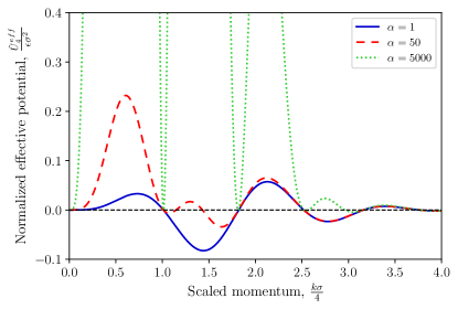
Figure 1: Plot of effective potential $\tilde{U}_{4}^{\rm eff}$ (Eq. (79)) normalized in units of $\epsilon\sigma^{2}$ as a function of scaled momentum $k\sigma/4$ for different temperature ratios $\alpha=\sigma^{2}\rho_{0}\epsilon/2k_{B}T$. The continuous (blue) line corresponds with $\alpha=1$, in the dashed (red) line $\alpha=50$. The extremely low temperature regime $\alpha=5000$ is depicted in the dotted (green) line.

We clearly see the appearance of “bands” in which $U_{4}^{\rm eff}(k)<0$ for a broad range of temperatures regime, allowing sound propagation in these regions. Also, there are dynamical phase transition points $k_{i}$, with $i=1,2,\dots$, where there are static solutions, representing periodic pattern formation at wavevectors where $U_{4}^{\rm eff}(k_{i})=0$. Near these singularities, the dispersion relation is

$$\!\omega_{j}\sim\left\{\begin{array}[]{lcl}\pm\sqrt{(-1)^{j}\sigma\left(k_{j}-k\right)}&\mbox{for}&k_{B}T\gtrsim\sigma^{2}\rho_{0}\epsilon\\ &&\\ \pm i\left|k_{j}-k\right|&\mbox{for}&k_{B}T<<\sigma^{2}\rho_{0}\epsilon\end{array}\right.$$ (80)

where $|k-k_{j}|\sigma<<1$. We observe dynamical phase transitions in the high temperature regime for special values of momenta. Very near the singularities, the dispersion relation has the same global properties that the previous dipolar case, i.e., square root singularities. In this way, the propagation of a pulse with a wide range of wave-vectors is a mixture of dispersive and dissipative regimes depending on the wave-vector spectrum.

VII Discussions and conclusions

We have demonstrated that the continuum limit of a system of interacting Brownian particles exhibits an exact symmetry, specifically an invariance under area-preserving diffeomorphisms. A significant physical consequence of this symmetry is the conservation of local vorticity.

By computing the generating functional using the saddle-point approximation plus Gaussian fluctuations, we have shown that the invariance under area-preserving diffeomorphisms manifests as a $U(1)$ gauge symmetry, leading to a gauge effective action for fluctuations around a homogeneous background. Equation (49) is the principal contribution of this paper. In this dual gauge theory, “electric charge” is interpreted as vorticity in the original particle system, while the magnetic field represents density fluctuations in the original model.

Using this formulation, we described the dynamics of density perturbations with a set of integro-differential equations analogous to Maxwell’s equations. The Gauss law arises from vorticity conservation, commonly referred to as the Kelvin circulation theorem in fluid mechanics. The equivalent of Faraday’s law is inherently satisfied due to gauge invariance. These equations are fundamentally dictated by symmetry. The system is completed with the dynamic equation (55), which incorporates information about the microscopic two-body potential of the original Brownian particle system.

The general solutions of this set of equations depend on the interplay between two-body interactions and thermal fluctuations. In the extremely low-temperature regime, the solutions for density fluctuations are damped, indicating that the homogeneous solution is stable and any weak perturbation diminishes to zero within a finite time scale, dependent on the wave vector of the perturbation. However, when thermal energy is comparable to or exceeds the typical interaction energy, more interesting phenomena such as sound propagation or static pattern formation may occur.

We solved the dynamical equations for various microscopic potentials. For a repulsive local potential, the only possible solution is an overdamped behavior with quadratic dispersion. Conversely, for a local attractive potential, there is a critical temperature above which the solutions are waves propagating in a dispersive medium with quadratic dispersion. Thus, the critical temperature demarcates two dynamical phases: in one phase, collective fluctuations are overdamped, while in the other, wave propagation is feasible.

We also explored some non-local repulsive interactions. In the case of a two-dimensional dipolar interaction $U(r)\sim 1/r^{3}$, we identified a dynamical phase transition, even for a purely repulsive potential, between more exotic phases. The competition between thermal fluctuations and microscopic interactions determines a wave vector scale $k_{0}$. At low temperatures or for wave vectors $k>k_{0}$, fluctuations are overdamped with dispersion proportional to $\omega\sim ik^{3}$. However, long-wavelength modes with $k<k_{0}$ can propagate without dissipation, with a dispersion $\omega\sim k^{5/2}$. Additionally, we examined the case of soft-core repulsive potentials, discovering a richer behavior. For exponential potentials decaying faster than a Gaussian, we found dynamical phase transitions at several specific wave vectors, bounding regions of overdamped and dispersive wave propagation. In this scenario, bands for wave propagation exist, whose width and structure are temperature-dependent.

Interestingly, in the non-local potential cases, near or at the dynamical phase transitions, the system may develop pattern formation. However, the dispersion relation near the transition is non-analytic, differing from the usual Swift-Hohenberg-Brazovskii models of pattern formation. For the cases studied, the square root singularity resembles the structure of non-Hermitian exceptional point singularities, suggesting the possibility of non-trivial topological structures in the dynamics of collective modes.

As emphasized, the emergent gauge symmetry appears in the weak fluctuation regime. It would be valuable to investigate the role of non-linearities, extending beyond this approximation. A systematic perturbative expansion, maintaining the invariance under area-preserving diffeomorphisms, could serve as a useful guide, as this is an exact symmetry of the system.

We hope to report on the non-linear response of interacting Brownian systems and its potential topological structures in the near future.

Appendix A Generating functional for Brownian particles

In this appendix we review the method of MSRJD that leads to the action of equation (5). The procedure essentially follows reference[22].

Consider the following system of stochastic equations

$$\frac{d{\bf r}_{i}(t)}{dt} =-\sum_{j\neq i}\bm{\nabla}_{r_{i}}U(|{\bf r}_{i}-{\bf r}_{j}|))+\bm{\xi}_{i}(t)$$ (81)

where $i=1,\ldots,N$. We use bold letters to indicate two-dimensional vector quantities. When necessary we use Greek index $\alpha,\beta=1,2$ represent the components of two dimensional vectors.

Eq. (81) is a set of overdamped Langevin equations of $N$ particles with positions ${\bf r}_{1},\ldots,{\bf r}_{N}$. The particles interact with a force between pairs given by

$${\bf F}_{i}(\{{\bf r}\})\equiv\bm{\nabla}_{r_{i}}\tilde{U}_{i}(\{{\bf r}\})\equiv\bm{\nabla}_{r_{i}}\sum_{j\neq i}U(|{\bf r}_{i}-{\bf r}_{j}|)).$$ (82)

${\bf F}_{i}(\{{\bf r}\})$ is the force exerted by the $j=1,\dots,N-1$ particles on the $i^{\rm th}$ particle by means of the potential $\tilde{U}_{i}(\{{\bf r}\})$. The notation $\{{\bf r}\}$ means the set of $N$ particles with positions ${\bf r}_{1},\ldots,{\bf r}_{N}$. The vector white noise $\bm{\xi}_{i}(t)$ is defined by the correlation functions,

$$\langle\xi_{\alpha,i}\rangle =0$$ (83)

$$\langle\xi_{i,\alpha}(t)\xi_{j,\beta}(t^{\prime})\rangle =2k_{B}T\delta_{ij}\delta_{\alpha\beta}\delta(t-t^{\prime})$$ (84)

where $k_{B}T$ is the diffusion constant that can be identified with the temperature of the environment.

In the following we build up the generating functional for correlation functions of eqs. (81).

The generating functional is given by

$$Z[\bm{\eta}] =\int\left(\prod_{i}{\cal D}{\bf r}_{i}(t)\right)\left\langle\delta\left({\bf O}\right)\det\left[\frac{\delta{\bf O}}{\delta{\bf r}}\right]\right\rangle_{{\bf\xi}}$$

$$\times\exp\{\int dt\left(\bm{\eta}_{i}\cdot{\bf r}_{i}\right)\}$$ (86)

where $\bm{\eta}_{i}$ are sources to compute correlation functions. The brackets $\langle\ldots\rangle_{\xi}$ mean the stochastic expected value. In Eq. (86), we have introduced the vector function

$$O^{\alpha}_{i}(t) =\frac{dr^{\alpha}_{i}(t)}{dt}+\nabla_{r_{i}}^{\alpha}\tilde{U}_{i}-\xi^{\alpha}_{i}(t)\;,$$ (87)

and the operator in the determinant is given by

$$\frac{\delta O^{\alpha}_{i}(t)}{\delta r_{j}^{\beta}(t^{\prime})} =\left\{\delta_{ij}\delta^{\alpha\beta}\frac{d~{}}{dt}+\nabla_{r_{j}^{\beta}}\nabla_{r_{i}^{\alpha}}\tilde{U}_{i}\right\}\delta(t-t^{\prime})\;.$$ (88)

The main goal of this formalism is to try to exactly compute the stochastic expectation value, in order to have a representation only in terms of the trajectories ${\bf r}_{i}(t)$. To do this we first exponenciate the delta function by using auxiliary vectors ${\bf A}_{i}$, in such a way that

$$\delta\left({\bf O}\right) =\int\left(\prod_{i}{\cal D}{\bf A}_{i}(t)\right)e^{i\int dt\sum_{i}A^{\alpha}_{i}O^{\alpha}_{i}}$$ (89)

We also exponenciate the determinant by using a set of independent vector Grassmann variables $\{\bm{\bar{\psi}}_{i},\bm{\psi}_{i}\}$ in such a way that

$$\det\left[\frac{\delta{\bf O}}{\delta{\bf r}}\right]=\int\left(\prod_{i}{\cal D}\bm{\bar{\psi}}_{i}{\cal D}\bm{\psi}_{i}\right)$$ (90)

$$\times\exp\left\{\int dtdt^{\prime}\sum_{ij}\bar{\psi}_{i}^{\alpha}(t)\frac{\delta O^{\alpha}_{i}(t)}{\delta r_{j}^{\beta}(t^{\prime})}\psi_{j}^{\beta}(t^{\prime})\right\}$$

With these tricks, the noises enter the exponential linearly an can be exactly integrated. Collecting all the noise terms we have,

$$\left\langle e^{-i\int dt\sum_{i}A_{i}^{\alpha}\xi_{i}^{\alpha}}\right\rangle_{\bm{\xi}}=e^{-\int dt\sum_{i}\left\{k_{B}T\left|{\bf A}_{i}\right|^{2}\right\}}$$ (91)

The next step is the integration over the Grassmann variables. Collecting all the terms in Grassmann variables we find,

$$\int\left(\prod_{i}{\cal D}\bm{\bar{\psi}}_{i}{\cal D}\bm{\psi}_{i}\right)\exp\left\{\int dt\sum_{i}\bm{\bar{\psi}}_{i}\cdot\frac{d\bm{\psi}_{i}}{dt}+\sum_{ij}\left(\bar{\psi}^{\alpha}_{i}\psi^{\beta}_{j}\nabla_{r_{j}^{\beta}}\nabla_{r_{i}^{\alpha}}\tilde{U}_{i}\right)\right\}=\exp\left\{\int dt\sum_{i}\frac{1}{2}\nabla^{2}_{r_{i}}\tilde{U}_{i}\right\}$$ (92)

The last result was obtained by using the relation

$$\left\langle\bar{\psi}^{\alpha}_{i}(t)\psi^{\beta}_{j}(t^{\prime})\right\rangle =\delta_{ij}\delta^{\alpha\beta}G_{R}(t-t^{\prime})$$ (93)

where $G_{R}(t-t^{\prime})$ is the retarded Green’s function of the operator $d/dt$ and $G_{R}(0)=1/2$ corresponding to the Stratonovich stochastic prescription.

After the noise and Grassmann variables integration we find

$$Z=\int\left(\prod_{i}{\cal D}{\bf r}_{i}(t){\cal D}{\bf A}_{i}(t)\right)\exp\left\{-\frac{1}{2k_{B}T}S\right\}$$ (94)

with

$$S =2k_{B}T\int dt\left\{\sum_{i}k_{B}T\left|{\bf A}_{i}\right|^{2}+iA_{i}^{\alpha}\left(\frac{dr^{\alpha}_{i}(t)}{dt}+\nabla_{r_{i}^{\alpha}}\tilde{U}_{i}\right)\right.$$

$$\left.-\frac{1}{2}\sum_{j\neq i}\nabla^{2}_{r_{i}}U\right\}\;.$$ (95)

The last step is to integrate over ${\bf A}_{i}$. This is a Gaussian integral and can be done without any difficulty.

Putting all terms together, the action in terms of ${\bf r}_{i}(t)$ can be cast in the following way,

$$S =\frac{1}{2}\int dt\sum_{i}\left\{\frac{d{\bf r}_{i}(t)}{dt}+\bm{\nabla}_{r_{i}}\tilde{U}_{i}\right\}^{2}$$

$$-k_{B}T\int dt\sum_{i}\nabla^{2}_{r_{i}}\tilde{U}(\{{\bf r}\})\;.$$ (96)

Equation (96) is the Onsager–Machlup action corresponding to the stochastic equation Eq. (81). The last term is the Jacobian of the variable transformation from $\bm{\xi}$ to ${\bf r}$, in the Stratonovich prescription.

It is more convenient to rewrite Eq. (96) in a Lagrangian form. To do this, we expand the square of the the first line of equation Eq. (96) and integrate by parts the cross term. We obtain

$$S =\int dt\sum_{i}\left\{\frac{1}{2}\left|\frac{d{\bf r}_{i}(t)}{dt}\right|^{2}+\frac{1}{2}\left|\bm{\nabla}_{r_{i}}\tilde{U}\right|^{2}-k_{B}T\nabla_{r_{i}}^{2}\tilde{U}\right\}$$

$$+\sum_{j}\left(\tilde{U}_{j}(t_{f})-\tilde{U}_{j}(t_{i})\right)\;.$$ (97)

The first line of this equation coincide with equation (5) in the main text. The second line is a constant term coming from the integration of total time derivatives. While this term is important to compute some equilibrium properties, it does not affect fluctuations given by the correlation functions of ${\rm r}_{i}$.

References

- Vicsek and Zafeiris [2012] T. Vicsek and A. Zafeiris, Collective motion, Physics Reports 517, 71 (2012), collective motion.
- Grzybowski et al. [2000] B. A. Grzybowski, H. A. Stone, and G. M. Whitesides, Dynamic self-assembly of magnetized, millimetre-sized objects rotating at a liquid–air interface, Nature 405, 1033 (2000).
- Glotzer and Solomon [2007] S. C. Glotzer and M. J. Solomon, Anisotropy of building blocks and their assembly into complex structures, Nature Materials 6, 557 (2007).
- Manoharan [2015] V. Manoharan, Colloids. colloidal matter: Packing, geometry, and entropy., Science , 1253751 (2015).
- Alberts et al. [2007] B. Alberts, A. Johnson, J. Lewis, M. Raff, K. Roberts, and P. Walter, Molecular Biology of The Cell, Vol. 230 (2007).
- Kawasaki [1994] K. Kawasaki, Stochastic model of slow dynamics in supercooled liquids and dense colloidal suspensions, Physica A: Statistical Mechanics and its Applications 208, 35 (1994).
- Dean [1996] D. S. Dean, Langevin equation for the density of a system of interacting langevin processes, Journal of Physics A: Mathematical and General 29, L613 (1996).
- Cugliandolo et al. [2015] L. F. Cugliandolo, P.-M. Déjardin, G. S. Lozano, and F. van Wijland, Stochastic dynamics of collective modes for brownian dipoles, Phys. Rev. E 91, 032139 (2015).
- Martin et al. [1973] P. C. Martin, E. D. Siggia, and H. A. Rose, Statistical dynamics of classical systems, Phys. Rev. A 8, 423 (1973).
- Janssen [1976] H.-K. Janssen, On a lagrangean for classical field dynamics and renormalization group calculations of dynamical critical properties, Zeitschrift für Physik B Condensed Matter 23, 377 (1976).
- de Dominicis [1976] de Dominicis, J. Physique Coll. 37, 377 (1976).
- Rieutord [2015] M. Rieutord, Fluid Dynamics: An Introduction, Graduate Texts in Physics (Springer International Publishing, 2015).
- Silvano and Barci [2024] N. Silvano and D. G. Barci, Emergent gauge symmetry in active brownian matter, Phys. Rev. E 109, 044605 (2024).
- Brazovskii [1975] S. A. Brazovskii, Phase transition of an isotropic system to a nonuniform state, Sov. Phys. JETP 41, 85 (1975).
- Swift and Hohenberg [1977] J. Swift and P. C. Hohenberg, Hydrodynamic fluctuations at the convective instability, Physical Review A 15, 319 (1977).
- BAHCALL and SUSSKIND [1991] S. BAHCALL and L. SUSSKIND, Fluid dynamics, chern-simons theory, and the quantum hall effect, International Journal of Modern Physics B 05, 2735 (1991), https://doi.org/10.1142/S0217979291001085 .
- Golden et al. [2010] K. I. Golden, G. J. Kalman, P. Hartmann, and Z. Donkó, Dynamics of two-dimensional dipole systems, Phys. Rev. E 82, 036402 (2010).
- Barci and Stariolo [2007] D. G. Barci and D. A. Stariolo, Competing interactions, the renormalization group, and the isotropic-nematic phase transition, Phys. Rev. Lett. 98, 200604 (2007).
- Barci and Stariolo [2009] D. G. Barci and D. A. Stariolo, Orientational order in two dimensions from competing interactions at different scales, Physical Review B 79, 075437 (2009).
- Aquino and Barci [2020] R. Aquino and D. G. Barci, Exceptional points in fermi liquids with quadrupolar interactions, Phys. Rev. B 102, 201110 (2020).
- Delfau et al. [2016] J.-B. Delfau, H. Ollivier, C. López, B. Blasius, and E. Hernández-García, Pattern formation with repulsive soft-core interactions: Discrete particle dynamics and dean-kawasaki equation, Phys. Rev. E 94, 042120 (2016).
- Moreno et al. [2015] M. V. Moreno, Z. G. Arenas, and D. G. Barci, Langevin dynamics for vector variables driven by multiplicative white noise: A functional formalism, Phys. Rev. E 91, 042103 (2015).