Corners and Islands in the S-matrix Bootstrap of the Open Superstring

Abstract

We bootstrap the Veneziano superstring amplitude in 10 dimensions from the bottom-up. Starting with the most general maximally supersymmetric Yang-Mills EFT, we input information about the lowest-lying massive states, which we assume contribute via tree-level exchanges to the 4-point amplitude. We show the following: (1) if there is only a single state at the lowest mass, it must be a scalar. (2) Assuming a string-inspired gap between the mass of this scalar and any other massive states, the allowed region of Wilson coefficients has a new sharp corner where the Veneziano amplitude is located. (3) Upon fixing the next massive state to be a vector, the EFT bounds have a one-parameter family of corners; these would correspond to models with linear Regge trajectories of varying slopes, one of which is the open superstring. (4) When the ratio between the massive scalar coupling and the ${\rm tr}F^{4}$ coefficient is fixed to its string value, the spin and mass of the second massive state is determined by the bootstrap and the Veneziano amplitude is isolated on a small island in parameter space. Finally, we compare with other recent bootstraps approaches, both the pion model and imposing Regge-inspired maximal spin constraints.

LCTP-24-10

1 Introduction and Summary of Results

The effective field theory (EFT) S-matrix bootstrap makes use of fundamental physical assumptions, such as unitarity, analyticity, and Froissart-like bounds, to constrain the allowed ranges for Wilson coefficients of higher-dimensional operators. The so-called “dual” formulation of the S-matrix bootstrap, which explicitly rules out coupling parameter space, has been applied to EFTs with a broad range of massless states, including permutation symmetric scalars, pions, photons, gluons, and gravitons Caron-Huot:2020cmc ; Arkani-Hamed:2020blm ; Chiang:2021ziz ; Albert:2022oes ; Caron-Huot:2022jli ; Fernandez:2022kzi ; Albert:2023jtd ; Alberte:2020bdz ; Henriksson:2021ymi ; Chowdhury:2021ynh ; Caron-Huot:2022ugt ; deRham:2022sdl ; Ma:2023vgc ; CarrilloGonzalez:2023cbf ; Berman:2023jys ; Chiang:2023quf . More recent implementations of this bootstrap technique study how additional physical assumptions about the massive spectrum can limit the allowed parameter space and yield new interesting features Albert:2023bml ; Haring:2023zwu . In particular, Albert:2023bml showed that for large-$N$ massless pion scattering, a new corner appeared in the allowed parameter space when information about the spin of the lowest-lying massive particles in the spectrum was included in the bootstrap.

Motivated by these recent results, we derive bounds on maximally supersymmetric Yang-Mills (SYM) EFTs using the S-matrix bootstrap combined with basic assumptions about the lowest massive states in the spectrum of the UV theory. We work at large rank of the gauge group so that multi-trace operators are suppressed and we assume weak coupling to suppress massless loops and ensure that the low-energy expansion is polynomial in the Mandelstam variables. Using maximal supersymmetry and locality, the general ansatz for the low-energy 4-point scattering amplitudes is

$$A(s,u)=-\frac{s}{u}+s^{2}\Big{[}a_{0,0}+a_{1,0}(s+u)+a_{2,0}(s^{2}+u^{2})+a_{2,1}su+\ldots\Big{]}\,.$$ (1.1)

The $a_{k,q}$ are the Wilson coefficients of the maximally supersymmetrized versions of the local single-trace operators ${\rm tr}(D^{2k}F^{4})$, e.g.

$$a_{0,0}~{}\leftrightarrow~{}{\rm tr}F^{4}\,,~{}~{}~{}~{}~{}~{}a_{1,0}~{}\leftrightarrow~{}{\rm tr}D^{2}F^{4}\,,~{}~{}~{}~{}~{}~{}a_{2,0}\,,a_{2,1}~{}\leftrightarrow~{}{\rm tr}D^{4}F^{4}\,,~{}~{}~{}\text{etc}.$$ (1.2)

There are two independent maximally supersymmetric ${\rm tr}D^{4}F^{4}$ operators, hence two coefficients are listed. From the low-energy perspective, without regard for the UV origin of the EFT, the Wilson coefficients $a_{k,q}$ in (1.1) could be any real numbers in units of some UV cutoff. The EFT S-matrix bootstrap allows us to compute upper and lower bounds on ratios of $a_{k,q}$.

One of the possible UV completions of the EFTs considered here is the open superstring, whose 4-point tree-level scattering process is given by the Veneziano amplitude Veneziano:1968yb ,

$$A^{\text{str}}(s,u)=-(\alpha^{\prime}s)^{2}\frac{\Gamma(-\alpha^{\prime}s)\Gamma(-\alpha^{\prime}u)}{\Gamma(1-\alpha^{\prime}(s+u))}\,.$$ (1.3)

Its low-energy $\alpha^{\prime}$-expansion,

$$A^{\text{str}}(s,u)=-\frac{s}{u}+s^{2}\bigg{(}\zeta_{2}\alpha^{\prime 2}+\zeta_{3}\alpha^{\prime 3}(s+u)+\zeta_{4}\alpha^{\prime 4}\big{(}s^{2}+u^{2}\big{)}+\frac{1}{4}\zeta_{4}\alpha^{\prime 4}su+\ldots\bigg{)}\,,$$ (1.4)

corresponds to a specific choice of the coefficients $a_{k,q}$ in (1.1). One of the goals of this paper is to bootstrap the Veneziano amplitude using as little physical input as possible.

In Berman:2023jys , we determined universal two-sided bounds on the Wilson coefficients $a_{k,q}$ of 4-dimensional $\mathcal{N}=4$ SYM EFT assuming the existence of a mass gap, but with no constraints imposed the UV spectrum; hence the notion of ‘universal bounds’. To compute the bounds, the $a_{k,q}$ are made dimensionless by scaling out powers of the mass gap and the bounds are derived for ratios of couplings

$$\bar{a}_{k,q}\equiv\frac{a_{k,q}}{a_{0,0}}\,.$$ (1.5)

The universal bounds determine an allowed region in the space of effective couplings $\bar{a}_{k,q}$. The Veneziano amplitude was found in the interior of the allowed region; it was not at any special place such as near a corner or cusp in the boundary. However, when the EFT bootstrap was combined with the additional constraint that the amplitude obeyed the string monodromy relations, it was found Berman:2023jys ; Chiang:2023quf that the two-sided bounds narrowed in on the $a_{k,q}$ values of the Veneziano amplitude (1.4). This was evidence for the earlier conjecture Huang:2020nqy that the open string is the unique amplitude compatible with the combined constraints of the EFT bootstrap and the string monodromy relations.

Isolating the low-energy expansion of the Veneziano amplitude with the monodromy relations has an interesting geometric interpretation, but it is not satisfactory to bootstrap the string amplitude by assuming one of its salient worldsheet properties. Instead, it would be much more desirable to find evidence of string theory (here specifically the Veneziano amplitude) from a more particle-based approach.

In this paper, we pursue a bottom-up EFT S-matrix bootstrap of the Veneziano amplitude in $D=10$ dimensions. The new “ingredient” in the bootstrap is information about the lowest massive states. In particular, the open string has a spin 0 state at mass-squared $1/\alpha^{\prime}$, a spin 1 state at $2/\alpha^{\prime}$, a spin 2 state at $3/\alpha^{\prime}$, etc, as its leading Regge trajectory. We find that even just assuming that the lowest-lying massive state is a scalar and that there is a suitable gap to the next (otherwise unspecified) state restricts the allowed parameter space so that the string is now found very near a corner in the resulting bounds. Moreover, we show that with input about only the lowest-mass state’s spin and coupling to the massless states relative to $a_{0,0}$, the Veneziano amplitude is isolated on islands that shrink in size as more constraints from higher-derivative operators are included.

More generally, we also examine the effects of basic low-spectrum input on the bounds in the EFT S-matrix bootstrap.

Setup and Summary of Results

We compute bounds on the ratios of Wilson coefficients in (1.5). This is done by using analyticity and the Froissart bound to derive dispersive representations for each $a_{k,q}$. Then those are used, together with unitarity, to formulate an optimization problem which is solved numerically with the semi-definite problem solver SDPB Simmons-Duffin:2015qma . This involves truncating the derivative expansion (1.1) to some finite order $k_{\text{max}}$ (corresponding to $2k_{\text{max}}+4$ derivative order); the numerical bounds get stronger with increasing $k_{\text{max}}$.

As context for the new bounds, the universal bounds in the $(\bar{a}_{1,0},\bar{a}_{2,0})$ plane (the coefficients of ${\rm tr}D^{2}F^{4}$ and of one of the ${\rm tr}D^{4}F^{4}$ operators, respectively) are simply Arkani-Hamed:2020blm ; Berman:2023jys :

$$\bar{a}_{1,0}^{2}\leq\bar{a}_{2,0}\leq\bar{a}_{1,0}\,.$$ (1.6)

This region (whose bounds happen to be independent of $k_{\text{max}}$) is shown in Figure 1 in teal. The region has two corners: the corner at $(0,0)$ corresponds to a model in which the ${\rm tr}F^{4}$ coupling dominates all other EFT couplings ($a_{0,0}\gg a_{k,q}$ for all $k>0$) and the $(1,1)$ corner is an (unphysical) model with an infinite spin tower at the mass gap.

The simplest assumption we can make about the massive spectrum is that the lowest mass states contribute to the 4-point amplitude $A(s,u)$ via simple pole exchanges, e.g.

(1.7)

for a particle with mass $M_{i}^{2}$, spin $\ell_{i}$, and coupling $g_{i}$ to the massless external states. To begin with, we only put in a single state, then subsequently, inspired by Albert:2023bml , two states.

Single-State Input. Suppose that the amplitude $A(s,u)$ has a pole at the mass gap $M_{\text{gap}}^{2}$ from the exchange of a massive spin-$\ell_{1}$ particle. We assume that, apart from this state, there are no other massive states until the “cutoff scale” $\mu_{c}M_{\text{gap}}^{2}$ for some $\mu_{c}>1$:

(1.8)

In (1.8), the circle at $s=M_{\text{gap}}^{2}$ indicates the simple pole in the $s$-channel of $A(s,u)$ while the thick blue line starting at $\mu_{c}M_{\text{gap}}^{2}$ indicates that we are completely agnostic about what occurs at or above the “cutoff scale” $\mu_{c}M_{\text{gap}}^{2}$: it can be poles, branch cuts, or both, so long as it is unitary.

Figure 1: This plot shows the allowed region for Wilson coefficients $\bar{a}_{1,0}$ and $\bar{a}_{2,0}$. Teal shows the region with unrestricted spectrum above the mass gap. Purple shows the allowed region for a scalar at the mass gap and no assumptions about the spectrum at and above $2M_{\text{gap}}^{2}$. In magenta is shown the allowed region when the cutoff is at $2M_{\text{gap}}^{2}$ and there is a non-zero spin state or no state at $M_{\text{gap}}^{2}$. The red dot corresponds to the Veneziano amplitude values for these coefficients and it sits very close to the corner in the purple bounds. The inset zooms in near the tip of the purple allowed region and shows the dependence of the bounds on the truncation parameter $k_{\text{max}}$ for $k_{\text{max}}=4,6,8,10,12,$ and $14$.

We first consider the choice of spin $\ell_{1}$. When $\ell_{1}=1,2,3,4,5$, we find that for $\mu_{c}>1$ there is no effect from adding in the spin state at the mass gap: the bounds will be the same as if no states were at the mass gap at all. Further, when we look at the maximal allowed relative couplings $|g_{\ell_{1}}|^{2}/a_{0,0}$ for an isolated state with spin $\ell_{1}>0$, we find that they decrease exponentially with $k_{\max}$, corresponding to including constraints from higher derivative operators. That selects the scalar as the only well-motivated choice for the lowest-mass state.

Setting $\ell_{1}=0$, the bounds depend on the choice of cutoff scale $\mu_{c}$. When $\mu_{c}\rightarrow 1$, we recover the full allowed parameter space, the teal region in Figure 1. However, as we increase $\mu_{c}$, the allowed region shrinks in size. Thinking of $M_{\text{gap}}^{2}$ as $1/\alpha^{\prime}$, we make the string-inspired choice $\mu_{c}=2$, so that the input is

(1.9)

The resulting allowed region, shown in purple in Figure 1, has a new corner at

$$\bar{a}_{1,0}\approx 0.7336\,,~{}~{}~{}~{}\bar{a}_{2,0}\approx 0.6598\,.$$ (1.10)

(These are the values for $k_{\text{max}}=14$; the change from $k_{\text{max}}=12$ to 14 is of order $10^{-4}$.) The corner values are close to the values for the Veneziano amplitude (1.4),

$$\bar{a}^{\text{str}}_{1,0}=\frac{\zeta_{3}}{\zeta_{2}}\approx 0.7308\,,~{}~{}~{}~{}\bar{a}^{\text{str}}_{2,0}=\frac{\zeta_{4}}{\zeta_{2}}\approx 0.6580\,,$$ (1.11)

shown as a red dot in Figure 1. Thus, we have found a new corner on the EFT bounds very close to the Veneziano amplitude! The only string-motivated input was the choice of gap $\mu_{c}=2$ in (1.9).

Single-State Input With Coupling. The lowest-mass state of the Veneziano amplitude is a scalar that couples to the massless states with (normalized) coupling

$$\bar{g}_{0}^{2}\equiv\frac{|g_{0}^{2}|}{a_{0,0}}=\frac{1}{\zeta_{2}}\,.$$ (1.12)

Let us pretend that this is a number that we have ‘measured’. If we enter this into the EFT bootstrap with spectrum assumptions, how much freedom is left in the EFT? Naively, one might think that fixing the spin and coupling of the lowest state does not amount to much information, but the EFT bootstrap says otherwise.

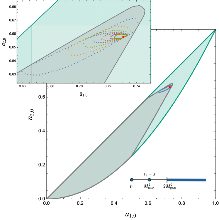
Figure 2: Island bounds bootstrapping the Veneziano amplitude (red dot). The gray region shows the $k_{\text{max}}=4$ bounds without the scalar coupling fixed. The blue island is $k_{\text{max}}=4$ bounds with the scalar coupling fixed to the string value (1.12). The zoomed inset shows that the island bounds continue to shrink for $k_{\max}=4,6,8,10,12,14,16$, narrowing in on the Veneziano amplitude.

First, we find that the cutoff scale $\mu_{c}$ above the lowest mass state (cf. the spectrum (1.8)) now has a maximum which we find converges to $\mu_{c}=2$ as $k_{\text{max}}$ increases (see Figure 7). Next, choosing this extremal value of the cutoff, $\mu_{c}=2$, we find that the allowed region becomes a small island around the Veneziano amplitude! This is illustrated for the $(\bar{a}_{1,0},\bar{a}_{2,0})$ plane in Figure 2. Moreover, as we increase the value of $k_{\text{max}}$, the size of the island shrinks, see the zoomed inset in Figure 2 for $k_{\text{max}}=4,6,8,10,12,14$, and $16$. (In the main text, we show the allowed islands for other Wilson coefficients.) Pushing to $k_{\max}=18$, we find

$$0.7261<\bar{a}_{1,0}<0.7333\,,~{}~{}~{}~{}~{}~{}~{}~{}~{}~{}~{}~{}~{}0.6569<\bar{a}_{2,0}<0.6598\,.~{}~{}~{}~{}~{}~{}$$ (1.13)

These values are within about 1% and 0.5% of the Veneziano string values (1.11), respectively. Thus, even with the minimal physical input of the lowest mass state, there is very little room for anything else in the maximally supersymmetric EFT.

Two-States Input. Let us approach the bootstrap of the open string from a different angle that does not require fixing any couplings. Consider the input of two massive states instead of one:

(1.14)

We find that the only non-trivial options for the spins are

$$\ell_{1}=0~{}~{}~{}~{}\text{and}~{}~{}~{}~{}\ell_{2}=1\,.$$ (1.15)

With this choice, we compute, for given choice of $\mu_{2}$, the maximum allowed value of the Wilson coefficient $\bar{a}_{1,0}$ and find that its value stays constant as $\mu_{c}$ increases from $\mu_{2}$ up to $\mu_{c}\approx 2\mu_{2}-1$ where it begins to drop off and reduce the allowed coupling space. This is illustrated in the plot of Figure 3 for a selection of $\mu_{2}$ choices, including the string-case of $\mu_{2}=2$ shown in dark green. The sudden drop in max($\bar{a}_{1,0}$) suggests that when $\mu_{c}$ is taken larger than $2\mu_{2}-1$ some amplitude with a massive state at $(2\mu_{2}-1)M_{\text{gap}}^{2}$ is ruled out.

Figure 3: Max($\bar{a}_{1,0}$) vs. the cutoff scale $\mu_{c}$ for $\mu_{2}=1$, $1.2$, $1.4$, $1.6$, $1.8$, $2$, $2.4$ and $(1.65)^{2}$ computed with $k_{\text{max}}=10$. Each curve has a corner near $\mu_{c}=2\mu_{2}-1$, suggesting a one-parameter family of models with a state of mass-squared $(2\mu_{2}-1)M_{\text{gap}}^{2}$. The dashed line corresponds to the upper bound on $\bar{a}_{1,0}$ with $\mu_{c}=\mu_{2}$, while the dotted line shows the max($\bar{a}_{1,0}$) for $\mu_{c}=2\mu_{2}-1$. The inset shows the location of the “corner theories” in the $(\bar{a}_{1,0},\bar{a}_{2,0})$-plane for a selection of $\mu_{2}$ values and with $\mu_{c}=2\mu_{2}-1$. The red curve in the inset corresponds to the Veneziano amplitude with varying $0\leq\alpha^{\prime}M_{\text{gap}}^{2}\leq 1$ and the red dot is for $\alpha^{\prime}M_{\text{gap}}^{2}=1$. Note that varying $\alpha^{\prime}M_{\text{gap}}^{2}$ is distinct from changing the Regge slope by varying $\mu_{2}$.

This would be compatible with a model whose spectrum has a linear Regge trajectory

$$M^{2}_{\ell}=(\mu_{2}-1)\ell+1\,.$$ (1.16)

Thus the bootstrap ‘discovers’ a one-parameter family of potentially interesting models with linear Regge trajectories (at least for $1<\mu_{2}\leq 2$ where the corner is quite sharp). The case with $\mu_{2}=2$ is the open string, but in this analysis it is not entirely clear what singles it out among the other ones. Apart from the case of Veneziano with $\mu_{2}=2$, we do not know a closed form of the generic ‘corner theory’ amplitudes.

The curves for $\text{max}(\bar{a}_{1,0})$ vs. $\mu_{c}$ appear to have another set of corners for $\mu_{c}>2\mu_{2}-1$ (see Figure 14.). If any theories ‘live’ there, they would have non-linear Regge trajectories, similar to those of mesons in real-world QCD and in the pion EFT studied in Albert:2023bml . If we select $\mu_{2}$ to take the same value as the mass gap between the $\rho$ and $f_{2}$ mesons, namely $(1.65)^{2}$, we find a corner in the bounds (when done in 4D) quite similar to that found in the pion model Albert:2023bml . There are some practical and qualitative similarities between our maximally supersymmetric model and the pion EFT of Albert:2022oes ; Albert:2023jtd ; Albert:2023bml that are likely responsible for this coincidence of numbers.

In this work, we have sought to assume only a minimum of well-motivated physical information about the spectrum. The guideline for the input has been to think about what data would be experimentally available had this been a “real-world” model. From that perspective, it seems reasonable to assume that the lowest EFT coefficient $a_{0,0}$ can been measured and that a scattering experiment can determine the mass, spin, and coupling $g_{0}^{2}$ of the lowest massive state. (This is certainly the case for pion scattering where much more information about the meson spectrum is also available.) For the maximally supersymmetric YM EFT, this basic data was sufficient to reduce the allowed space of Wilson coefficients to a small island around the Veneziano amplitude. Such strong constraints may not be found in bootstraps of generic EFTs with less symmetry. Also, experimentally, there would be error bars on the measurements of masses and couplings, so one would have to smear over any islands resulting from the bootstrap to take these uncertainties into account. Nonetheless, one can think of our setup as a very simple toy model for the application of the S-matrix bootstrap to more realistic cases.

Outline. In Section 2, we discuss the constraints of maximal supersymmetry, the dispersive representation, and some simple analytic bounds. The input of spectral information is described and put in the context of known UV completions. We also outline the numerical implementation.

Section 3 begins with a bootstrap of the possible spins for the state with the lowest mass in the spectrum. We then discuss the string at the corner of the bounds (e.g. Figure 1) and the string islands (Figure 2.)

Next, in Section 4, we argue that input of specific states can give corners in the bounds of Wilson coefficients and we show how that motivates particular spectrum input for the bootstrap. We examine this first for the bootstrap of the Veneziano amplitude and next more generally to find the one-parameter of corner theories from Figure 3. We notice that, for larger mass gaps, the bounds have secondary corners which would correspond to models with non-linear Regge trajectories. We compare one such corner with the pion-bootstrap.

In Section 5, we show that the bounds obtained with one- and two-state input are very similar to those computed by imposing a fixed leading Regge trajectory on the full spectrum.

We discuss the results and outlook in Section 6. The appendices contain additional details about the numerical implementation (Appendix A) as well as some results of bootstrapping the Veneziano amplitude using information about the two lowest massive states and their couplings (Appendix B).

Note Added: As this paper was being completed, we learned about similar ideas being pursued in the forthcoming paper AKRboot by Albert, Knop, and Rastelli with complementary results for the open string bootstrap.

2 SUSY Constraints and the Dispersive Representation

In this section, we show how to implement the constraints of maximal supersymmetry and generalize the derivation of the dispersive represention in Berman:2023jys to $D$-dimensions. We then describe the general set up for adding the lowest-massive states into the spectrum. Finally we discuss the spectrum and couplings of the massive states exchanged in the open string tree amplitude.

2.1 Supersymmetry Constraints

In $D=4$ dimensions, maximal super Yang-Mills theory has $\mathcal{N}=4$ supersymmetry and the self-dual supermultiplet of massless states consists of the gluons, the four gluinos, and three pairs of complex scalars. The $\mathcal{N}=4$ SUSY Ward identities imply that all 4-point single-trace amplitudes are proportional to each other. Thus, without loss of generality, we can focus on the color-ordered scalar amplitude

$$A(s,u)=A[zz\bar{z}\bar{z}]\,,$$ (2.1)

where $z$ and $\bar{z}$ is any pair of conjugate complex scalars of the $\mathcal{N}=4$ massless supermultiplet. It was shown in Berman:2023jys that the $\mathcal{N}=4$ SUSY Ward identities requires the amplitude (2.1) to take the form $A(s,u)=s^{2}f(s,u)$, where $f(u,s)=f(s,u)$. This is a SUSY version of crossing symmetry. The most general ansatz for the EFT expansion of this amplitude is then

$$A^{\text{EFT}}(s,u)=-\frac{s}{u}+s^{2}\sum_{0\leq q\leq k}a_{k,q}\,s^{k-q}\,u^{q}\,~{}~{}~{}~{}\text{with}~{}~{}~{}~{}a_{k,k-q}=a_{k,q}\,.$$ (2.2)

The constraints $a_{k,k-q}=a_{k,q}$ follows from the SUSY crossing condition $f(u,s)=f(s,u)$. The first term is the gluon-exchange in the $u$-channel of the leading order 2-derivative SYM theory. The polynomial terms in the Mandelstam variables $s$ and $u$ are in 1-to-1 correspondence with (linear combinations of) the on-shell $\mathcal{N}=4$ compatible local operators of the schematic form ${\rm tr}(D^{2k+4}z^{2}\bar{z}^{2})\xleftrightarrow{\text{SUSY}}{\rm tr}(D^{2k}F^{4})$. The $a_{k,q}$ are Wilson coefficients for these operators, e.g. $a_{0,0}$ is the coefficient of ${\rm tr}(F^{4})$, $a_{1,0}=a_{1,1}$ is the coefficient of ${\rm tr}(D^{2}F^{4})$ and so on, as outlined in (1.2). The subscript $k$ on $a_{k,q}$ is associated with the derivative order and $q$ labels distinct operators of the same order.

Consider now $2\rightarrow 2$ scattering amplitudes in maximally supersymmetric Yang-Mills theory in $D>4$ spacetime dimensions. If we restrict the external states to a 4D subspace, the states can be decomposed into the massless $\mathcal{N}=4$ supermultiplet and the amplitudes obey the 4D $\mathcal{N}=4$ SUSY Ward identities. We can then reuse all the above 4D results.

Thus, in $D$ dimensions, we consider a four-point amplitude $A(s,u)$ whose restriction to a 4D subspace gives the scalar amplitude (2.1). The dependence on the spacetime dimension $D$ enters via the partial wave decomposition

$$A(s,u)=\sum_{\ell=0}^{\infty}\,n_{\ell}^{(D)}a_{\ell}(s)\,G_{\ell}^{(D)}\Big{(}1+\frac{2u}{s}\Big{)}\,,$$ (2.3)

in which $a_{\ell}(s)$ is the spectral density, $n_{\ell}^{(D)}$ is a dimension-dependent normalization Correia:2020xtr ; Caron-Huot:2020cmc ,

$$n_{\ell}^{(D)}=\frac{(4\pi)^{D/2}(D+2\ell-3)\Gamma(D+\ell-3)}{\pi\Gamma(\frac{D-2}{2})\Gamma(\ell+1)}\,,$$ (2.4)

and $G_{\ell}^{(D)}$ are the $D$-dimensional Gegenbauer polynomials, which can be written in terms of the hypergeometric function ${}_{2}{F}_{1}$ as

$$G^{(D)}_{\ell}(x)\equiv{}_{2}{F}_{1}\left(-\ell,\ell+D-3,\frac{D-2}{2},\frac{1-x}{2}\right)\,.$$ (2.5)

Thus, the internally exchanged particles with spin ‘know’ that they ‘live’ in $D$ dimensions.

2.2 Dispersive Representation

The EFT S-matrix bootstrap assumptions are unitarity (specifically positivity since we are working at tree-level), analyticity, and the Froissart-like bounds that $A(s,u)/s^{2}\rightarrow 0$ for $|s|\rightarrow\infty$ at fixed $u<0$ (and similarly at fixed $t<0$). In addition, we assume a mass gap, large rank of the gauge group (e.g. only single-trace operators considered), and weak couplings so that any running of the couplings is suppressed and we can work at tree-level in the EFT. More detailed statements of the assumptions are given in Section 3 of Berman:2023jys .

Using a standard contour deformation argument, it was shown in Berman:2023jys that all the Wilson coefficients $a_{k,q}$ of the amplitude (2.2) have a dispersive representation. Generalizing to $D$-dimensions and redefining all $a_{k,q}$ to be dimensionless, we have

$$a_{k,q}=\sum_{\ell=0}^{\infty}\int_{M^{2}_{\textrm{gap}}}^{\infty}\frac{dM^{2}}{M^{2}}\,n_{\ell}^{(D)}\rho_{\ell}(M^{2})\left(\frac{M_{\text{gap}}^{2}}{M^{2}}\right)^{k+D/2}v^{(D)}_{\ell,q}\,,~{}~{}~{}~{}~{}\rho_{\ell}(M^{2})\geq 0\,.$$ (2.6)

Unitarity ensures positivity of the spectral density $\rho_{\ell}(s)=s^{(D-4)/2}\text{Im}\big{(}a_{\ell}(s)\big{)}$. In $D=4$, the $v^{(4)}_{\ell,q}$ are the coefficients of the Legendre polynomials $P_{\ell}\big{(}1+2\delta\big{)}=\sum_{q=0}^{\ell}v_{\ell,q}\delta^{q}$. In general $D$ dimensions, the numbers $v_{\ell,q}^{(D)}$ are similarly derived from the Gegenbauers (2.5) as

$$v_{\ell,q}^{(D)}=(-1)^{q}\frac{1}{q!}\frac{\partial^{q}}{\partial x^{q}}\,{{}_{2}}F_{1}\left(-\ell,\ell+D-3,\frac{D-2}{2},x\right)\bigg{|}_{x=0}\,.$$ (2.7)

Importantly, all $v^{(D)}_{\ell,q}$ are non-negative. Our analysis is in $D=10$, so henceforth we drop the superscript ^(D) with the understanding that $v_{\ell,q}$ are the 10-dimensional coefficients unless otherwise stated.

Changing integration variable to $y=M^{2}/M_{\text{gap}}^{2}$ in (2.6), we find

$$a_{k,q}\,=\,\sum_{\ell=0}^{\infty}\int_{1}^{\infty}dy\,f_{\ell}(y)\,y^{-k}v_{\ell,q}~{}=~{}\Big{\langle}y^{-k}v_{\ell,q}\Big{\rangle}_{1}\,\ ,$$ (2.8)

where $f_{\ell}(y)=y^{-(D/2+1)}n_{\ell}^{(D)}\rho_{\ell}(M_{\text{gap}}^{2}y)\geq 0$ and we have introduced the compact notation

$$\Big{\langle}Q\Big{\rangle}_{\mu}=\sum_{\ell=0}^{\infty}\int_{\mu}^{\infty}dy\,f_{\ell}(y)\,Q(\ell,y)\,.$$ (2.9)

If $\mu>1$, the dispersion integral starts above the mass gap, i.e. the lowest mass-scale to enter the dispersive integral is $\mu M_{\text{gap}}^{2}$.

Null Constraints. The SUSY crossing constraints $a_{k,k-q}=a_{k,q}$ from (2.2) place constraints on the spectral density. It is further constrained by relations derived from the dispersion relations at constant $t$ (as opposed to constant $u<0$ used to derive (2.6)). These constraints are collectively referred to as the “null constraints” and they play a key role for the numerical computation of the bounds. We provide the explicit expressions for the null constraints in Appendix A.1.

2.3 Simple Analytic Bounds

It follows directly from the integral (2.8) and the non-negativity of the $v_{\ell,q}$ that $a_{k,q}\geq 0$ for all $k$ and $q$, and that

$$a_{k,q}\geq a_{k^{\prime},q}~{}~{}~{}~{}\text{for}~{}~{}~{}~{}k<k^{\prime}\,.$$ (2.10)

Together with the SUSY crossing constraint, $a_{k,k-q}=a_{k,q}$, one can show Berman:2023jys that $a_{k,q}\leq a_{0,0}$ for all $k$ and $q$. Thus, the lowest-dimension operator, ${\rm tr}F^{4}$, has an effective coupling $a_{0,0}$ that, in units of the mass gap $M_{\text{gap}}^{2}$, is greater than all other Wilson coefficients. It is therefore natural to bound the higher-derivative couplings relative to $a_{0,0}$:

$$\bar{a}_{k,q}\equiv\frac{a_{k,q}}{a_{0,0}}~{}~{}~{}\text{for which}~{}~{}~{}0\leq\bar{a}_{k,q}\leq 1\,.$$ (2.11)

One can derive the analytic bounds Berman:2023jys

$$\bar{a}_{k,0}^{k^{\prime}/k}\leq\bar{a}_{k^{\prime},0}\leq\bar{a}_{k,0}~{}~{}~{}~{}\text{for~{}~{} $k\leq k^{\prime}$}\,.$$ (2.12)

The case of $k=1$ and $k^{\prime}=2$ was given in (1.6) and shown as the teal region in Figure 1.

Scaling of Bounds. The bounds in (2.11) and (2.12) were derived from the dispersive representation (2.8). If we change the lower bound on the dispersion integral from $1$ to $\mu>1$, i.e. if we define

$$a_{k,q}^{(\mu)} =\Big{\langle}y^{-k}v_{\ell,q}\Big{\rangle}_{\mu}\,,$$ (2.13)

then it follows from a scaling of the dispersion integral that

$$\max\big{(}\bar{a}_{k,q}^{(\mu)}\big{)}=\frac{1}{\mu^{k}}\max\big{(}\bar{a}_{k,q}^{(1)}\big{)}~{}~{}~{}~{}\text{with}~{}~{}~{}~{}\bar{a}_{k,q}^{(\mu)}=\frac{a_{k,q}^{(\mu)}}{a_{0,0}^{(\mu)}}\,.$$ (2.14)

The bounds (2.11) and (2.12) then become

$$0\leq\bar{a}_{k,q}^{(\mu)}\leq\mu^{-k}~{}~{}~{}~{}\text{and}~{}~{}~{}~{}(\bar{a}_{k,0}^{(\mu)})^{k^{\prime}/k}\leq\bar{a}_{k^{\prime},0}^{(\mu)}\leq\mu^{k-k^{\prime}}\bar{a}_{k,0}^{(\mu)}~{}~{}~{}\text{for $k\leq k^{\prime}$}\,.$$ (2.15)

For example, with $\mu=2$ we get

$$0\leq\bar{a}_{1,0}^{(2)}\leq\frac{1}{2}~{}~{}~{}~{}\text{and}~{}~{}~{}~{}(\bar{a}_{1,0}^{(2)})^{2}\leq\bar{a}_{2,0}^{(2)}\leq\frac{1}{2}\,\bar{a}_{1,0}^{(2)}\,.$$ (2.16)

This is relevant for the projection of the allowed region to the $(a_{1,0},a_{2,0})$ plane and is shown as the magenta-colored region in Figure 1.

2.4 Spectrum Input

In the Introduction, we discussed the specification of explicit low-mass states in the EFT bootstrap. We now detail how this is implemented, reviewing the ideas proposed in Albert:2022oes ; Albert:2023bml . The contribution from a state with spin $\ell_{i}$ and mass $M_{i}$ to an $s$-channel pole is captured by the residue of the 4-point amplitude as

$$\raisebox{-19.91692pt}{\includegraphics[width=79.6678pt]{Figures/poleterm.pdf}}~{}~{}~{}\longrightarrow~{}~{}~{}\text{Res}_{s=M_{i}^{2}}A_{4}=-|g_{i}|^{2}\,G_{\ell_{i}}\Big{(}1+\frac{2u}{M_{i}^{2}}\Big{)}\,,$$ (2.17)

where $g_{i}$ is the coupling between the massive state and the two massless external states $z$.

The residue appears in the spectrum as a delta-function, i.e.

$$(M^{2})^{(4-D)/2}\rho_{\ell}(M^{2})\,\supset\,|g_{i}|^{2}\delta\Big{(}M^{2}-M_{i}^{2}\Big{)}\,.$$ (2.18)

Thus, including an explicit spectrum up to a given cutoff scale $\mu_{c}M_{\text{gap}}^{2}$ means we can analytically integrate (2.8) for each Wilson coefficient $a_{k,q}$ up to the scale set by $\mu_{c}$. For the spectrum of simple poles illustrated in Figure 4, we get

$$a_{k,q}=\sum_{n=1}^{N}\sum_{\ell=0}^{\infty}\frac{|g_{\ell,\mu_{n}}|^{2}}{\mu_{n}^{k+3}}v_{\ell,q}+\Big{\langle}y^{-k}v_{\ell,q}\Big{\rangle}_{\mu_{c}}\,.$$ (2.19)

The couplings $|g_{\ell,\mu_{n}}|^{2}$ enter the bootstrap as additional parameters in the optimization problem. They can be specified explicitly, extremized, or left as free parameters of the optimization. The numerical implementation is briefly discussed in Section 2.6 with further details relegated to Appendix A.

Figure 4: The analytic structure of the amplitude $A(s,u)$ with $N$ poles located on the positive real $s$-axis at $s=\mu_{n}M_{\text{gap}}^{2}$ for $n=1,2,\dots,N$. For $s\geq\mu_{c}M_{\text{gap}}^{2}$ we are agnostic about the form of the spectral density.

As an example, for a spin $\ell_{1}$ state with coupling $g_{0}$ at the mass gap, i.e. $\mu_{1}=1$, and a spin $\ell_{2}$ state with coupling $g_{1}$ at $\mu_{2}$ gives

$$a_{k,q}=|g_{0}|^{2}v_{\ell_{1},q}+\frac{|g_{1}|^{2}}{\mu_{2}^{k+3}}v_{\ell_{2},q}+\Big{\langle}y^{-k}v_{\ell,q}\Big{\rangle}_{\mu_{c}}\,.$$ (2.20)

The Gegenbauer coefficients $v_{\ell,q}$ vanish unless $\ell\geq q$. Naively, that means that a spin $\ell_{i}$ state only contributes to Wilson coefficients with $q\leq\ell_{i}$; however, the SUSY crossing constraints $a_{k,k-q}=a_{k,q}$ makes this more subtle. For example, a spin 0 state contributes explicitly to $a_{1,0}=|g_{0}|^{2}+\Big{\langle}y^{-k}v_{\ell,0}\Big{\rangle}_{\mu_{c}}$, but also indirectly to $a_{1,1}=\Big{\langle}y^{-k}v_{\ell,1}\Big{\rangle}_{\mu_{c}}$ via the SUSY crossing constraints $a_{1,0}=a_{1,1}$.

The factors of $\mu_{n}^{-k-3}$ in (2.19) and (2.20) arise from the redefined spectral function, $f_{\ell}(y)\propto y^{-(D/2+1)}\rho_{\ell}\big{(}M_{\text{gap}}^{2}y\big{)}$, the factor of $(M^{2})^{(4-D)/2}$ that appears in the relationship between $\rho_{\ell}$ and the couplings (2.18), and the integrand factor of $y^{-k}$ with $y=M_{\text{gap}}^{2}/M^{2}$. Their appearance implies that the contributions from higher-mass states are significantly suppressed, especially for higher values of $k$. This offers some intuition of why the input of the lowest-mass state(s) has a substantial effect on the bootstrap bounds. We discuss this further in Section 3.

It should be noted that any explicitly input spin-$\ell$ state for the $s$-channel of the amplitude $A[zz\bar{z}\bar{z}]$ is part of a supermultiplet. The other states of that supermultiplet are exchanged in other component amplitudes proportional to $A[zz\bar{z}\bar{z}]$ by supersymmetry.

2.5 UV Models: Veneziano, IST, and SSE

Veneziano Spectrum and Couplings

$$\begin{array}[]{c|ccccccc}n\backslash\ell&0&1&2&3&4&5\\ \hline\cr 1&1&0&\cdots\\ 2&0&2&0&\cdots\\ 3&0&0&3&0&\cdots\\ 4&0&\frac{4}{33}&0&\frac{128}{33}&0&\cdots\\ 5&\frac{5}{2376}&0&\frac{625}{1404}&0&\frac{15625}{3432}&0&\cdots\\ \vdots\end{array}\hskip 36.98866pt\raisebox{-85.35826pt}{ \includegraphics[width=170.71652pt]{Figures/ReggeTrajVeneziano.pdf}}$$

Figure 5: The table shows the 10D values of $|g_{\ell,\mu_{n}}|^{2}$, as defined in (2.17), in units of $1/\alpha^{\prime}$ for the scalar Veneziano amplitude (1.3). $\ell$ labels the spin and the $n$th level has mass $n/\alpha^{\prime}$. The plot of $M^{2}$ vs. spin shows the Regge trajectories for the Veneziano amplitude. Note that the scalar coupling at mass level $n=3$ is $\frac{3(10-D)}{8(D-1)\alpha^{\prime}}$, so it vanishes in $D=10$.

Consider the Veneziano amplitude in $D\geq 4$ dimensions. With the external states restricted to a 4D subspace, the Veneziano amplitude can be written

$$A^{\text{str}}(s,u)=A^{\text{str}}[zz\bar{z}\bar{z}]=-(\alpha^{\prime}s)^{2}\frac{\Gamma(-\alpha^{\prime}s)\Gamma(-\alpha^{\prime}u)}{\Gamma(1-\alpha^{\prime}(s+u))}\,,$$ (2.21)

which was the form presented in (1.3). The low-energy expansion of the Veneziano amplitude was given in (1.4).

The gamma-functions in the numerator of (2.21) give simple poles whenever their arguments are 0 or a negative integer. In the $s$-channel, the poles are at $s=m_{n}^{2}=n/\alpha^{\prime}$ for $n=0,1,2,3,\dots$, but the $s=0$ pole is eliminated by the overall SUSY factor $s^{2}$; in $\mathcal{N}=4$ SYM, there is no massless pole in the $s$-channel of the amplitude $A^{\text{str}}[zz\bar{z}\bar{z}]$ (but there is a gluon exchange in the $u$-channel).

The residues of the first few massive poles show that the exchanged states are as follows: a scalar at $1/\alpha^{\prime}$, a vector at $2/\alpha^{\prime}$, a spin 2 particle at $3/\alpha^{\prime}$ etc. The tower of spin $n$ states at $n/\alpha^{\prime}$ lie on the first Regge trajectory, illustrated in Figure 5. In addition, there are towers of daughter trajectories starting at $4/\alpha^{\prime}$. Also listed in Figure 5 are the couplings $g_{\ell,n}$ of each state as computed via (2.17) for $D=10$. When we compare bootstrap results to the Veneziano amplitude, we take the mass gap to be given by the lowest-mass state of the Venaziano amplitude, i.e. $M_{\text{gap}}^{2}=1/\alpha^{\prime}$.

Infinite Spin Tower (IST)

The amplitude

$$A_{m^{2}}^{\text{IST}}(s,u)=-\frac{s}{u}+\frac{s^{2}}{\left(m^{2}-s\right)\left(m^{2}-u\right)}\,,$$ (2.22)

has a infinite tower of spins, all with the same mass $m^{2}$. This is not expected to be physical, but it is also not ruled out by the universal EFT bounds. With $m^{2}=\mu M_{\text{gap}}^{2}$, the low-energy expansion gives effective couplings,

$$\bar{a}_{k,q}^{\text{IST}}=\frac{1}{\mu^{k-2}}\,,$$ (2.23)

for all $k$ and $q$. Thus, in the $(\bar{a}_{1,0},\bar{a}_{2,0})$-plane, the IST amplitudes saturate the lower bound in (1.6) as they have $\bar{a}_{2,0}=\bar{a}_{1,0}^{2}$. Hence, the lower bound on the teal region in Figure 1 is matched by IST amplitudes with mass $m^{2}=\mu M_{\text{gap}}^{2}$. The corner at the $(1,1)$ in that plot is the IST amplitude with $m^{2}=M_{\text{gap}}^{2}$, whereas the corner at (1/2,1/4) of the purple region in Figure 1 is the IST with $m^{2}=2M_{\text{gap}}^{2}$.

SUSY Scalar Exchange (SSE)

The amplitude

$$A_{m^{2}}^{\text{SSE}}(s,u)=-\frac{s}{u}+\frac{s^{2}}{2M_{\text{gap}}^{2}}\left(\frac{1}{m^{2}-s}+\frac{1}{m^{2}-u}\right)\,$$ (2.24)

grows as $s^{2}$ for $|s|\rightarrow\infty$ and therefore just barely fails to satisfy our Froissart bound. A modification of the amplitude (see Albert:2022oes ) can remedy this and, as such, we can consider $A^{\text{SSE}}$ as a borderline case. The low-energy expansion identifies the values of the Wilson coefficients as $a_{0,0}=1$, $a_{k,0}=a_{k,k}=1/(2m^{2(k+1)}M_{\text{gap}}^{2})$ for $k>0$, and $a_{k,q}=0$ for $0<q<k$. In Figure 1, the SSE amplitude with $m^{2}=M_{\text{gap}}^{2}$ is located at $(\bar{a}_{1,0},\bar{a}_{2,0})=(1/2,1/2)$ on the diagonal upper bound on the allowed region. The rest of the diagonal is the SSE amplitude with mass greater than $M_{\text{gap}}^{2}$ (for $\bar{a}_{1,0}<1/2$) or a linear combination of the SSE and the IST (for $1/2<\bar{a}_{1,0}<1$).

Coulomb Branch

On the Coulomb branch, the massive states couple quadratically to the massless states, so they cannot enter as tree-level exchange of the 4-point amplitudes, but they contribute via loops. Thus, the simplest Coulomb branch amplitude has a branch cut starting at $4m^{2}$, where $m$ is the mass of the massive $W$-supermultiplet. Our spectrum input assumes poles from the lowest-mass states and explicitly excludes branch cut below the cutoff $\mu_{c}M_{\text{gap}}^{2}$. For that reason, the Coulomb branch does not play any significant role in the bootstrap analysis of this paper.

2.6 Numerical Implementation

The method for turning the dispersive representation of the Wilson coefficients with positivity bound $\rho_{\ell}(M^{2})\geq 0$ into a linear optimization problem has been discussed in detail in the literature; see for example Caron-Huot:2020cmc ; Albert:2022oes ; Berman:2023jys . Here, we briefly describe the essential components so we can fix notation, following Section 4 in Berman:2023jys . To start, we allow only a finite number of spins contained in a spin vector $\vec{\ell}$ to appear in our dispersive sum and write a vector equation

$$\vec{V} =\sum_{\ell\in\vec{\ell}}\int_{0}^{1}dy\,f_{\ell}(y)\,\vec{E}_{\ell,y}$$ (2.25)

where $\vec{V}$ contains, as its first element, $a_{0,0}$, and $a_{k,q}$ as its second element when $\bar{a}_{k,q}$ is the coefficient we wish to extremize. The subsequent entries contain any expression we wish to set to zero, that is, $a_{k^{\prime},q^{\prime}}-Ra_{0,0}$ to fix the value fo $\bar{a}_{k^{\prime},q^{\prime}}$ to $R$, or $|g_{\ell,\mu_{n}}|^{2}-Ga_{0,0}$ fixing $|\bar{g}_{\ell,\mu_{n}}|^{2}=|g_{\ell,\mu_{n}}|^{2}/a_{0,0}$ to the value $G$. The vector $\vec{V}$ also includes all linearly independent null constraints from SUSY crossing (given explicitly in Appendix A.1) up to some $k_{\max}$ which truncates the derivative expansion to $2k_{\text{max}}+4$ derivative order. Emperically, we find that the bounds only change substantially at even $k_{\max}$, and so do not give bounds at odd values. The entries of $\vec{E}_{\ell,y}$ are chosen so that (2.25) matches the dispersive representation of the coefficients and null constraints. The vertex representation (2.25) can brought to the standard form of a linear or semi-definite optimization problem Caron-Huot:2020cmc ; Albert:2022oes ; Berman:2023jys .

As noted, the spin sum has to be truncated to a finite list of spins. Rather than including all spins up to some $\ell_{\max}$, it turns out to be computationally advantageous to instead include all spins up to some cutoff between 50 and 200, then use a sparse set of spins that includes both even and odd spins up to some much higher maximum. The bounds depend on the spin list $\vec{\ell}$, which is chosen empirically for each $k_{\max}$ by ensuring that the bounds do not change more than an acceptable amount (say, less than $\mathcal{O}(10^{-6})$) when the maximum spin is increased or the spin list includes a denser set of spins. Using this kind of spin vector was initially suggested in Albert:2022oes and greatly reduces the computational time needed to bound coefficients at large $k_{\max}$.

3 Single State Input

In this section, we consider bounds on amplitudes with a single massive state at the mass gap and then no other contributions up to a second cutoff scale. We assume the state contributes to the amplitude $A(s,u)$ via a tree-level exchange, as in Section 2.4. First, we show that the single state at the mass gap has to be scalar. We then describe how leveraging this information, along with one additional piece of string-inspired input, reduces the allowed space in a way that singles out the Veneziano amplitude as special.

3.1 Bootstrapping the Spectrum at the Mass Gap

Consider a spin $\ell_{1}$ particle at the mass gap. Using (2.19), we have

$$\raisebox{-21.33955pt}{\includegraphics[width=156.49014pt]{Figures/InputMassGen.pdf}}\hskip 28.45274pta_{k,q}=|g_{\ell_{1},1}|^{2}v_{\ell,q}+\Big{\langle}y^{-k}v_{\ell,q}\Big{\rangle}_{\mu_{c}}\,.$$ (3.1)

The coupling $|g_{\ell_{1},1}|^{2}$ is a variable that can be optimized on the same footing as the Wilson coefficients.

To examine the different options for the choice of spin $\ell_{1}$, we compute the maximum allowed value for the coupling of the massive state to the massless states relative to the ${\rm tr}F^{4}$ coupling $a_{0,0}$. Specifically, we maximize

$$|\bar{g}_{\ell_{1},1}|^{2}=\frac{|g_{\ell_{1},1}|^{2}}{a_{0,0}}\,.$$ (3.2)

To enforce that the spin $\ell_{1}$ state is the only state at the mass gap, we set the cutoff $\mu_{c}M_{\text{gap}}^{2}$ to be above the mass gap, e.g. $\mu_{c}>1$. For non-zero spin, $\ell_{1}>0$, we find that the maximum allowed value of $|\bar{g}_{\ell_{1},1}|^{2}$ decreases quickly as the cutoff $\mu_{c}$ increases. It is expected that all non-zero spin couplings go to zero as $\mu_{c}\rightarrow\infty$ because there is no single-spin $\ell>0$ exchange amplitude (analogous to (2.24)) compatible with the Froissart bound.

However, even just above the mass gap, e.g. for $\mu_{c}=1.1$, we find that $\text{max}\big{(}|g_{\ell_{1},1}|^{2}\big{)}$ decreases towards 0 exponentially fast with increasing $k_{\text{max}}$. This is illustrated in Figure 6 for $\ell_{1}=1,2,3,4,5$, indicating that in the limit of including constraints from arbitrarily high orders in the derivative expansion, $k_{\text{max}}\rightarrow\infty$, having a single state with non-zero spin is not allowed: its coupling to the massless states is exponentially suppressed. This implies that bounds on the Wilson coefficients $\bar{a}_{k,q}$ will not be sensitive to a non-zero spin state at the mass gap.

In contrast, for a spin 0 state, the maximum allowed coupling $|\bar{g}_{0,1}|^{2}$ is constant as a function of $k_{\text{max}}$ and has no suppression, as also shown in Figure 6 for $\mu_{c}=1.1$. Thus, we conclude that if the spectrum only has one state at the mass gap $M_{\text{gap}}^{2}$, that state has to be a scalar!

We also checked the generalized scenario in which we allowed two states at the mass gap, a scalar and either a spin one or two exchange. There, with $\mu_{c}=1.1$, the maxima of the allowed couplings for the spin 1 and 2 states are larger than those given on the right side of Figure 6, but they are still are decreasing exponentially with $k_{\max}$.

Figure 6: Left: The maximum of the coupling $|\bar{g}_{1,1}|^{2}$ of a spin-1 particle at the mass gap with three different values of $\mu_{c}$ as a function of $k_{\text{max}}$. Right: The maximum of $|\bar{g}_{\ell,1}|^{2}$ for the given spins and $\mu_{c}=1.1$. Both plots illustrate that a state with spin $\ell_{1}>0$ at the mass gap $M_{\text{gap}}$ has a coupling that is suppressed exponentially with increasing $k_{\max}$.

Studying the scalar coupling as a function of $\mu_{c}$ shows that the maximal value of $|\bar{g}_{0,1}|^{2}$ decreases monotonically. At $\mu_{c}=1$, it takes the value $(777-1120\ln(2))\approx 0.6752$, which matches the scalar coupling of the IST model (2.22) and as $\mu_{c}\rightarrow\infty$, $|\bar{g}_{0,1}|^{2}$ asymptotes toward $1/2$, which is the normalized scalar coupling of the SSE model (2.24). There are no particular features in that plot that points to any special values of the cutoff $\mu_{c}$.

3.2 Cornering Veneziano

A single scalar exchanged at the mass gap exactly matches the first massive state at $M_{\text{gap}}^{2}=1/\alpha^{\prime}$ in the open string spectrum. We know from Section 2.5 there are no other states that contribute to the Veneziano amplitude until $2M_{\text{gap}}^{2}=2/\alpha^{\prime}$, so we now impose this string-inspired cutoff $\mu_{c}=2$:

$$\raisebox{-19.91692pt}{\includegraphics[width=156.49014pt]{Figures/SingleMassInput.pdf}}\hskip 28.45274pta_{k,q}=|g_{0}|^{2}v_{0,q}+\Big{\langle}y^{-k}v_{\ell,q}\Big{\rangle}_{2}\,.$$ (3.3)

Leaving $|g_{0}|^{2}$ as a free parameter for the maximization/minimization of the Wilson coefficient $\bar{a}_{2,0}$ as a function of $\bar{a}_{1,0}$, we obtain Figure 1. The purple region corresponds to the bounds on the $\bar{a}_{2,0}$ vs. $\bar{a}_{1,0}$ region with this spectrum. The region outside the purple but within the teal bounds is where there must be more than a scalar in the spectrum below $M^{2}=2M_{\text{gap}}^{2}$. Moreover, the region within the purple space but outside of the magenta region must have a nontrivial contribution from a scalar at the mass gap $M_{\text{gap}}^{2}$.

As discussed in the Introduction, the string values of $a_{k,q}$ are close to the boundary of the allowed region. Quantitatively, the maximal values of $\bar{a}_{1,0}$ and $\bar{a}_{2,0}$ differ from the string coefficients by just $2.8\times 10^{-3}$ and $2.3\times 10^{-3}$ for $k_{\max}\geq 14$.

In Figure 1, the inset shows that, upon zooming in close to the string value, the bounds sharpen as we increase $k_{\max}$. Note that the lower bound on $\bar{a}_{2,0}$ appears to be moving extremely slowly with $k_{\max}$. Though the space does become slightly more constrained, there is no clear evidence that it is shrinking fast enough that the string would lie directly on the boundary even as $k_{\text{max}}$ is taken very large. It is possible that further physics input would be needed to truly corner the string and we discuss examples of this in the following sections.

We picked the gap $\mu_{c}=2$ solely based on input from the string spectrum. It is natural to ask what happens for other values of $\mu_{c}$. We discuss this further in Section 4.3.

3.3 Veneziano Island

Next we experiment with fixing the coupling $g_{0}$ of the massive scalar to the massless states from (3.3). We let the cutoff $\mu_{c}M_{\text{gap}}^{2}$ be general, but pick the string-value (see table in Figure 5) for the coupling:

$$|\bar{g}_{0}^{\text{str}}|^{2}=\frac{|{g}_{0}^{\text{str}}|^{2}}{a_{0,0}^{\text{str}}}=\frac{1}{\zeta_{2}}\,,$$ (3.4)

We then have

$$\raisebox{-22.76219pt}{\includegraphics[width=170.71652pt]{Figures/IntroSpectrum2.pdf}}\hskip 28.45274pt\bar{a}_{k,q}=\frac{v_{0,q}}{\zeta_{2}}+\frac{1}{a_{0,0}}\Big{\langle}y^{-k}v_{\ell,q}\Big{\rangle}_{\mu_{c}}\,.$$ (3.5)

Since $v_{0,q}=1$ for $q=0$ and is zero for $q>0$, only the $a_{k,0}$ coefficients ‘see’ the contribution from the scalar directly.

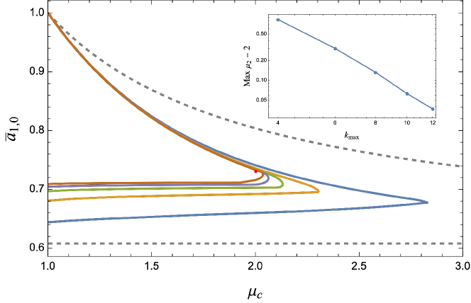
Figure 7: $\bar{a}_{1,0}$ vs. $\mu_{2}$ with $|\bar{g}_{0}|^{2}=1/\zeta_{2}$ for $k_{\max}=4,6,8,10,12$. The gray dashed lines are the naive bounds on $\bar{a}_{1,0}$ from (3.9). The inset shows on a log-log scale the maximum allowed value of the cutoff $\mu_{2}$ converging to 2 as $k_{\max}$ is increased.

Analytic Bounds. Due to this explicit contribution to the $a_{k,0}$ coefficients, fixing the coupling to the string value as in (3.4) gives a non-zero lower bound on $\bar{a}_{k,0}$ since the high energy integral in (3.5) must be non-negative:

$$\bar{a}_{k,0}\geq\frac{1}{\zeta_{2}}\approx 0.608\,.$$ (3.6)

We can also extract an analytic expression for a new upper bound on $\bar{a}_{k,0}$. The high energy integral obeys scaling arguments like those discussed in Section 2.3, i.e.

$${\max}\Big{(}\Big{\langle}y^{-k}v_{\ell,0}\Big{\rangle}_{\mu_{c}}\Big{)}={\max}\Big{(}\frac{1}{\mu_{c}^{k}}\Big{\langle}y^{-k}v_{\ell,0}\Big{\rangle}_{1}\Big{)}\,.$$ (3.7)

Normally, $\frac{1}{a_{0,0}}\Big{\langle}y^{-k}v_{\ell,0}\Big{\rangle}_{1}$ would be bounded from above by 1, but because we have already subtracted out a contribution of size $1/\zeta_{2}$, we must find that in the $\mu_{c}\rightarrow 1$ limit of (3.5),

$$\frac{1}{a_{0,0}}\Big{\langle}y^{-k}v_{\ell,0}\Big{\rangle}_{1}\leq 1-\frac{1}{\zeta_{2}}\,.$$ (3.8)

Combining (3.6) and (3.7), we arrive at the two-sided bounds

$$\frac{1}{\zeta_{2}}\leq\bar{a}_{k,0}\leq\frac{1}{\zeta_{2}}+\frac{1-1/\zeta_{2}}{\mu_{c}^{k}}.$$ (3.9)

Thus, for any $\mu_{c}>1$, the value of $\bar{a}_{k,0}$ is increasingly squeezed from above and below for larger values of $k$ and $\lim_{k\rightarrow\infty}a_{k,0}=1/\zeta_{2}$. Notably, for the Veneziano amplitude, we have

$$\bar{a}_{k,0}=\frac{\zeta_{k+2}}{\zeta_{2}}\rightarrow\frac{1}{\zeta_{2}}~{}~{}~{}\text{for}~{}~{}~{}k\rightarrow\infty\,.$$ (3.10)

It is rather surprising that simple low-energy input, as the mass, spin, and coupling of the lowest-mass state in the spectrum has such significant impact on the coupling of high-dimension operators: at large $k$, we find that only the string values of the $\bar{a}_{k,0}$ coefficients are allowed!

Numerical Bounds.  For lower values of $k$, analytic bounds (3.9) are not as constraining as for higher $k$. However, it turns out that that the SDPB bounds are substantially stronger. Figure 7 shows the upper and lower bounds on $\bar{a}_{1,0}$ as a function of $\mu_{c}$. The analytic bounds (3.9) are shown for comparison as the dashed curves. Importantly, the upper and lower numerical bounds show that there are no solutions to the bootstrap above a certain $k_{\text{max}}$-dependent value of the cutoff $\mu_{c}$. The existence of this maximal cutoff means that there must be a state either at or below that cutoff in order for there to be a unitary theory with the chosen $|\bar{g}_{0}|^{2}$. The inset gives evidence that the maximum allowed value of $\mu_{c}$ is 2 in the limit of large $k_{\text{max}}$. We take this maximum to be the “bootstrap” choice for $\mu_{c}$. Thus, by fixing the coupling to the scalar, we have bootstrapped the choice of cutoff $\mu_{c}=2$ from Section 3.1.

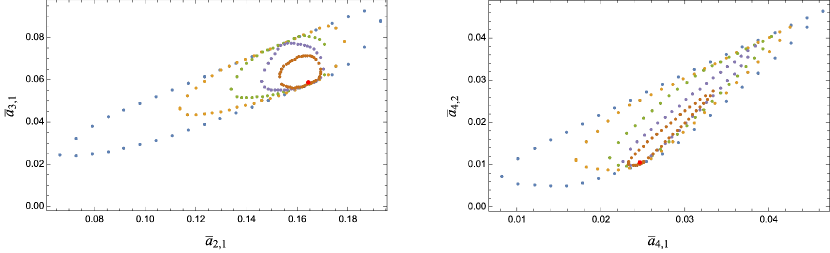
Figure 8: Bounds on the allowed regions in the $(\bar{a}_{2,1},\bar{a}_{3,1})$ and $(\bar{a}_{4,1},\bar{a}_{4,2})$ planes for $k_{\max}=4,6,8,10,12$. We assume a scalar at $M_{\text{gap}}^{2}$ with coupling $|\bar{g}_{0}|^{2}=1/\zeta_{2}$ and no other state until $2M_{\text{gap}}^{2}$.

Continuing with $\mu_{c}=2$, we find that the allowed region in the $(\bar{a}_{1,0},\bar{a}_{2,0})$ coupling space is reduced to the shrinking islands displayed in Figure 2 of the Introduction. As noted, the scalar input affects the only the $\bar{a}_{k,0}$ coefficients directly, but we also find islands in other projections, for example for the $(\bar{a}_{2,1},\bar{a}_{3,1})$-plane and the $(\bar{a}_{4,1},\bar{a}_{4,2})$-plane shown in Figure 8. In all these cases, the allowed coupling region shrinks to an island around the string, much smaller than the region that was allowed by our universal bounds or even the bounds with the naive constraint in (3.9). More generally, we find that the upper and lower bounds for all coefficients $\bar{a}_{k,q}$ with $k\leq 4$ narrow in on their string values with increasing $k_{\max}$, as illustrated in Figure 9.

Figure 9: Two-sided bounds on the eight lowest-dimension Wilson coefficients $\bar{a}_{k,q}$ computed with a single scalar input at $M_{\text{gap}}^{2}$, with the coupling $|\bar{g}_{0}|^{2}$ fixed to the string value (3.4), and no other states until $2M_{\text{gap}}^{2}$. The bounds indicate convergence towards the string values (red dashed lines) as $k_{\max}$ increases, shown here for $k_{\max}$ between $4$ and $18$.

The fact that $\mu_{c}=2$ appears to be the maximal value for $\mu_{c}$ for the choice of $|\bar{g}_{0}|^{2}=1/\zeta_{2}$ implies that there must be some contribution to the high energy spectrum that lives at $M^{2}=2M_{\text{gap}}^{2}$. We can determine what that contribution is by performing similar tests to those described by Figure 6. We assume the most simple input, that there is a single particle exchange of spin $\ell$ at $\mu_{2}=2$, set the cutoff mass to various values slightly above $\mu_{2}=2$, then evaluate the maximal $|\bar{g}_{\ell,2}|^{2}$. We find that at $k_{\max}=10$, there are no unitary solutions to the optimization problem unless the single particle input is a vector. Once we know that, we can insert the vector, then test whether other particles can live at $\mu_{2}=2$ by again evaluating the maximal $|\bar{g}_{\ell,2}|^{2}$ (still with the scalar at the mass gap input with its coupling fixed by (3.4), but with the vector at $\mu_{2}=2$ having unfixed coupling). We find strong evidence that the couplings to states with $\ell>2$ would vanish at large $k_{\max}$. For the scalar, though, the maximal $|\bar{g}_{0,2}|^{2}$ appears to decrease more slowly at higher $k_{\max}$, at least to the point we tested, so there is no obvious bootstrap-inspired reason to rule out its existence. The Veneziano amplitude has no scalar contribution at $\mu_{2}=2$, so it is not clear the bootstrap can directly determine the Veneziano spectrum without either more input or higher $k_{\max}$ information. In the next section, we study how the low-mass spectrum affects the bounds.

4 Multiple State Input

We now take a step back from the Veneziano-centric analysis in Sections 3.2 and 3.3 in order to understand better how state input affects the coupling bounds and selects different “bootstrap trajectories”.

4.1 Bifurcation from State Input

Consider the following input to the bootstrap:

$$\raisebox{-20.20146pt}{\includegraphics[width=156.49014pt]{Figures/IntroSpectrum1.pdf}}\hskip 22.76228pta_{k,q}=|g_{0}|^{2}v_{\ell_{1},q}+\frac{|g_{1}|^{2}}{\mu_{2}^{k+3}}v_{\ell_{2},q}+\Big{\langle}y^{-k}v_{\ell,q}\Big{\rangle}_{\mu_{c}}\,.$$ (4.1)

We do not fix the couplings $g_{0}$ or $g_{1}$; they are variables in the optimization problem.

The Wilson coefficient $a_{1,0}$ is sensitive to all spins, so we study the maximum allowed value of $\bar{a}_{1,0}$ as a function of $\mu_{2}$ and the cutoff $\mu_{c}$. We allow $\mu_{c}$ to extend all the way down to the mass gap, $\mu_{c}=1$, in order to track the effect of the state insertion at $\mu_{2}$. The results we describe here are computed with $\mu_{2}=2$ but are qualitatively the same for other values of $\mu_{2}$, as will be discussed further in Section 4.3.

Figure 10: Max($\bar{a}_{1,0}$) vs. the cutoff scale $\mu_{c}$ at $k_{\max}=14$ for listed state insertions. Starting at the upper right corner, the bound on $\bar{a}_{1,0}$ follows two different trajectories depending on whether a scalar is assumed at $M_{\text{gap}}^{2}$ or not. A similar bifurcation happens based on what states are allowed at $2M_{\text{gap}}^{2}$. Near $3M_{\text{gap}}^{2}$ there is a corner in the bounds, indicating that another bifurcation is possible when a specific state is inserted at that point. We tested other spins up to $\ell=5$ and found results similar to Figure 6. The dashed gray lines extrapolate the bounds to $\mu_{c}\rightarrow\infty$ (in the large $k_{\max}$ limit). As indicated, two of these curves are expected to go to the Single Scalar Exchange (SSE) amplitude from Section 2.5 at $M_{\text{gap}}^{2}$ and $2M_{\text{gap}}^{2}$, respectively.

Figure 10 shows the maximum value of $\bar{a}_{1,0}$ vs. $1/\mu_{c}$. We start in the upper right corner where with $\text{max}(\bar{a}_{1,0})=1$ for $\mu_{c}=1$; this is the maximum from the basic universal bounds (2.11). The diagonal line from (1,1) to (0,0) corresponds to the basic scaling from eq. (2.14), which gives $\text{max}(\bar{a}_{1,0}^{(\mu_{c})})=\frac{1}{\mu_{c}}\text{max}(\bar{a}_{1,0}^{(1)}))=1/\mu_{c}$ when there are no states at all below $\mu_{c}$. This upper bound on $\bar{a}_{1,0}$ is saturated by the Infinite Spin Tower (IST) amplitude from Section 2.5.

As we increase $\mu_{c}$, we find two separate paths: one for which the state at the mass gap is a scalar and one when it is not. The latter is simply the diagonal in Figure 10; hence including a spin $\ell\neq 0$ state at the mass gap is the same as not allowing it at all! This is equivalent to the finding in Section 3.1 that non-scalar input at the mass gap have highly suppressed couplings. In contrast, a scalar at the mass gap gives the higher trajectory in Figure 10.

When $\mu_{c}$ reaches $\mu_{2}=2$, there is a bifurcation due to the explicit state input at that point. Following first the diagonal path, a new trajectory splits off for $\ell_{2}=0$ only. This is simply a repeat of the split of paths at (1,1). For the upper path with a scalar at the mass gap ($\ell_{1}=0$), the bifurcation is more interesting. The maximum of $\bar{a}_{1,0}$ is insensitive to any other state than a vector $\ell_{2}=1$. When we input a vector state at $\mu_{2}=2$, the maximum of $\bar{a}_{1,0}$ stays nearly constant until close to $\mu_{c}=3$. Around $\mu_{c}=3$, the maximum suddenly decreases and asymptotes back to the trajectory of having only the scalar input at the mass gap. The inset on the lower right of Figure 10 zooms in on the curve near the corner and illustrates its dependence on increasing $k_{\max}$. It shows that the constant value corner is nearly saturated by $k_{\max}=10$.

The fact that $\text{max}(\bar{a}_{1,0})$ stays nearly constant and then suddenly decreases is a sign of another potential bifurcation point. As seen at $\mu_{2}=2$, bifurcations and the resulting corners in the bounds are associated with state inputs. However, unlike the other splittings, this new corner does not occur at a place that we have explicitly inserted a state. Instead, it appears naturally as we increase the cutoff, so it can be interpreted as the bootstrap discovering that a state is “missing” at $3M_{\text{gap}}^{2}$!

From the Veneziano amplitude, we know that the missing state at $3M_{\text{gap}}^{2}=3/\alpha^{\prime}$ is a spin 2 state. For further comparison with the string, the dashed red line in Figure 10 shows the value, $\bar{a}_{1,0}^{\text{str}}=\zeta_{3}/\zeta_{2}$ for Veneziano. This is close to the nearly flat bound with the scalar and vector input. If we include a spin 2 state at $3M_{\text{gap}}^{2}$, then $\text{max}(\bar{a}_{1,0})$ has to stay above the string value, so this generates a new path which is nearly horizontal until the cutoff reaches the next “missing” state.

One could continue adding states this way to understand which states and where to insert them preserves the nearly horizontal behavior of the $\text{max}(\bar{a}_{1,0})$. Rather than adding more states in by hand, we now discuss the bootstrap with two states input.

4.2 Veneziano Bootstrap With 2-State Input

A main take-away from the previous section is that with a scalar at $M_{\text{gap}}^{2}$ and a vector at $2M_{\text{gap}}^{2}$, the bootstrap tells us we should maximally push the cutoff to $\sim 3M_{\text{gap}}^{2}$ if no other states are inserted. Setting $\mu_{c}=3$, we can then proceed to compute the resulting allowed regions for the Wilson coefficients. This gives a somewhat sharper corner in the $(\bar{a}_{1,0},\bar{a}_{2,0})$-plane near the Veneziano amplitude than for the single scalar input in Figure 1. Such plots are shown in Appendix B where we also experiment with fixing both the scalar and vector couplings to get even smaller islands than in Figure 2.

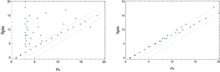
Figure 11: The $k_{\max}=14$ extremal spectrum for the maximal $\bar{a}_{1,0}$ with the string spectrum inserted up to $\mu_{c}=3$ with (right) and without (left) additional maximal spin assumptions. The first two states in the string spectrum are enforced (black) and the rest of the spectrum is generated by SDPB (blue). The gray dashed lines correspond to the lowest Regge trajectories of the string spectrum.

Rather than using the approach from Figure 10 to determine higher-mass state insertions, we can use the built-in SDPB tool that can extract the spectrum for a theory, assuming it has only tree-level exchanges. Given that we find the maximal $\bar{a}_{1,0}$ to be nearly flat, we can expect it to track the actual value the bootstrapped model, and hence SDPB should be able to extract the spectrum from maximizing $\bar{a}_{1,0}$. As shown on the left in Figure 11, for any $\mu_{c}$ between two and three, we find that the SDPB spectra all share the same important feature: a spin two state near $3M_{\text{gap}}^{2}$, a spin three state around $4M_{\text{gap}}^{2}$, and a spin four state close to $5M_{\text{gap}}^{2}$, following closely the leading string Regge trajectory. At higher masses, we find that the SDPB states are not quite the string trajectory, but instead there are states that are slightly larger in mass than the string spectrum.

SDPB does not appear to find the “daughter” Regge trajectories. Instead, the SDPB spectra tends to have many low-mass states with large spin, i.e. states that lie below the first “physical” linear Regge trajectory and mimic infinite spin tower theories. (This was also observed in Albert:2023bml .) These are similar to the states which have maximal couplings that decrease exponentially as we increase $k_{\max}$, as we discussed in Section 3.1. We can ad hoc eliminate such “too high spin” states by requiring that there be a minimal mass allowed for states with a particular spin, a condition recently studied in Haring:2023zwu . In particular, we assume that the spectrum obeys a Regge-like constraint

$$\ell\leq\gamma\left(\frac{M^{2}}{M_{\text{gap}}^{2}}-1\right)\,,$$ (4.2)

where $\gamma$ is the first Regge slope. Upon imposing this condition, the spectrum, shown on the right hand side of Figure 11, is much cleaner and has more states along the first Regge trajectory and a few states along the second Regge trajectory, yet it also has many additional states that do not lie at stringy locations. This may be a finite-$k_{\text{max}}$ effect.

4.3 New Linear Regge Trajectories

We have seen that we obtain nontrivial constraints from the bootstrap when we insert a scalar at the mass gap $M_{\text{gap}}^{2}$ and a spin 1 state at twice that mass gap, i.e. at $M^{2}/M_{\text{gap}}^{2}=\mu_{2}=2$. However, this choice of mass for the second state is not unique.

As an example, we choose the vector to be at $1.5M_{\text{gap}}^{2}$ instead of $2M_{\text{gap}}^{2}$, i.e. pick $\mu_{2}=1.5$. The result of repeating the analysis from Section 4.1 is shown in Figure 12, which is qualitatively similar to Figure 10. The horizontal path now has a corner at $\mu_{c}=2$. We find that inserting a spin two state at $2M_{\text{gap}}^{2}$ is the choice that allows the horizontal trajectory to continue to be flat for higher $\mu_{c}$, but now there is a new dropoff at $\mu_{c}$ near 2.5. Figure 12 includes the path with a spin 3 state allowed at $2.5M_{\text{gap}}^{2}$. This set of states corresponds to a linear Regge trajectory with slope $1/2$ instead of the string choice of 1.

More generally, we can examine the behavior of $\text{max}(\bar{a}_{1,0})$ for the spectrum

(4.3)

as a function of $\mu_{c}$. In that case, we find corners near $2\mu_{2}-1$. This is illustrated at on the right of Figure 12, which is the same as Figure 3, though with $1/\mu_{c}$ on the horizontal axis. There is a sharp corner for the lower values of $\mu_{2}$, but it becomes more rounded as $\mu_{2}$ increases.

The corner at $2\mu_{2}-1$ suggests, as we saw for the $\mu_{2}=1.5$ case, that some model has a spin 2 state at $(2\mu_{2}-1)M_{\text{gap}}^{2}$. This indicates a linear Regge trajectory of the form:

$$\frac{M^{2}_{\ell}}{M_{\text{gap}}^{2}}=(\mu_{2}-1)\ell+1\,.$$ (4.4)

This family of linear Regge trajectories has a spin $0$ state at the mass gap, a spin one state at $\mu_{2}$, and a spin two state at $2\mu_{2}-1$, and predicts a spin 3 state at $3\mu_{2}-2$. Extracting the spectrum from SDPB for $\mu_{2}=1.2$ corroborates this linear Regge trajectory, as shown in the left of Figure 13. As in Figure 11, the SDPB spectrum contains several other states with high spin. We can input the Regge constraint (4.2) with $\gamma=5$ to match the $\mu_{2}=1.2$ trajectory. The result is shown on the right in Figure 13, but it is a bit unclear how exactly to interpret these spectrum plots.

Figure 12: Left: Max($\bar{a}_{1,0}$) vs. the cutoff mass $\mu_{c}$ at $k_{\max}=10$ for $\mu_{2}=3/2$. As in Figure 10, dashed gray lines indicate expected behavior of these curves as $\mu_{c}\rightarrow\infty$ in the large $k_{\max}$ limit. Right: Max($\bar{a}_{1,0}$) vs. $1/\mu_{c}$ at $k_{\max}=10$ for $\mu_{2}=1$, $1.2$, $1.4$, $1.6$, $1.8$, $2$, $2.4$ and $(1.65)^{2}$. This figure is the same as Figure 3, but the horizontal axis is inverted.

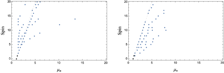
Figure 13: The $k_{\max}=14$ extremal spectrum for the maximal $\bar{a}_{1,0}$ with a scalar at $\mu_{1}$, a vector at $\mu_{2}=1.2$ and no other state up to $\mu_{c}=1.4$ when the maximal spin assumptions are (right) and are not (left) enforced. The first two states are input (black) and the rest of the spectrum is generated by SDPB (blue). The gray dashed line corresponds to a linear trajectory with slope 5.

We briefly turn to the question of which amplitudes may correspond to the 1-parameter family of corner theories. Parameterizing them by their Regge slope with $\gamma=1/(\mu_{2}-1)$, we know three explicit cases: $\gamma=1$ is the Veneziano amplitude. For $\gamma=0$, we must have $\ell\leq 0$ for all finite mass, so only the scalar exchange is allowed in the $s$-channel. This corresponds to the scalar exchange amplitude (2.24). Finally, for the $\gamma\rightarrow\infty$ limits, particles of all spin are allowed for any $M^{2}\geq M_{\text{gap}}^{2}$, so the maximal $\bar{a}_{1,0}$ will match the generic bounds, that is, will be $\bar{a}_{1,0}=1$. The same will be true for all other Wilson coefficients, so the corner theory corresponds to the Infnite Spin Tower amplitude (2.22). The corners in Figure 3 indicates that there could be a 1-parameter family of unitary 4-point amplitudes that connect these three cases. However, for no other choices of $\gamma$ do we have a closed form expression for the amplitude that corresponds to the corner.

There has been recent progress in studying general variations on the Veneziano amplitude Cheung:2022mkw ; Geiser:2022exp ; Cheung:2023adk ; Cheung:2023uwn , but these amplitudes do not have linear Regge trajectories with slope $\neq 1$ and they are not supersymmetrizable. One possible way forward is something similar to the proposal in Cheung:2023uwn for an amplitude with a fully customizable spectrum, but the discussion there is based on the non-supersymmetric open string amplitude and so does not appear to be compatible with our bounds.

Other possible variations involve modifying the Veneziano amplitude in the style of the Lovelace-Schapiro amplitude Lovelace:1968kjy ; Shapiro:1969km ; Bianchi:2020cfc :

$$A(s,u)\sim-(\alpha^{\prime}s)^{2}\frac{\Gamma(\alpha_{0}-\alpha^{\prime}s)\Gamma(\alpha_{1}-\alpha^{\prime}u)}{\Gamma(b+\alpha^{\prime}(s+u))}\,,$$ (4.5)

so the slope is controlled by $\alpha^{\prime}/\alpha_{0}$. However, any such simple modification results in an infinite tower of negative norm states or tachyons. One could, in principle, try to subtract off the negative norm states from the amplitude, but this would still not necessarily lead to an expression for the amplitude any more exact than trying to read off Wilson coefficients from these corner plots. Further, it is difficult to see how an amplitude with such a form could approach the scalar exchange or infinite spin tower amplitudes in their appropriate limits.

4.4 Non-Linear Regge Trajectories?

One interesting feature of the maximally supersymmetric model is that, while it has nothing to do with 4D real-world QCD or the large-$N$ pion EFT, the optimization problems we solve are almost identical to those solved for the pions in Albert:2022oes ; Fernandez:2022kzi ; Albert:2023bml . The large-$N$ pion model has no massless poles and an Adler zero, so, instead of (1.1), the generic ansatz for the low-energy color-ordered amplitude is

$$A^{\text{pion}}(s,u)=b_{1,0}(s+u)+b_{2,0}(s^{2}+u^{2})+b_{2,1}su+\ldots$$ (4.6)

Other than the absence of the $a_{0,0}$ coefficient, the amplitude has the same degrees of freedom as (1.1). Where the pion amplitude has crossing symmetry $A^{\text{pion}}(u,s)=A^{\text{pion}}(s,u)$, the SYM amplitude has the SUSY-induced crossing relation $A^{\text{SUSY}}(s,u)=s^{2}f(s,u)$ with $f(u,s)=f(s,u)$. The null constraints from these crossing relations are equivalent, and, since these numerical bootstrap procedures relies on imposing null constraints, the optimization problems are mathematically very similar. The only technical difference is that the additional factor of $s^{2}$ in $A^{\text{SUSY}}$ means that we can write convergent dispersion relations for all of our Wilson coefficients, while in the large $N$ pion bootstrap, the $b_{k,k}$ coefficient is inaccessible at every level $k$. Therefore, crossing relations such as $b_{k,k}-b_{k,0}=0$ cannot be imposed. These simple equalities are related to the $\mathcal{X}_{k,q}^{\ell,y}$ and $\mathcal{Y}_{k,q}^{\ell,y}$ null relations described in Appendix A.1, so while we can impose the relations for all $k$ and $q$, only some can be enforced in the pion model. At $k_{\max}=2$, for example, crossing symmetry implies the following high energy integrals vanish,

$$\left\langle\mathcal{X}^{\ell,y}_{1,0}\right\rangle\,,\left\langle\mathcal{X}^{\ell,y}_{2,0}\right\rangle\,,\left\langle\mathcal{Y}^{\ell,y}_{0,0}\right\rangle\,,\left\langle\mathcal{Y}^{\ell,y}_{1,0}\right\rangle\,,\left\langle\mathcal{Y}^{\ell,y}_{2,0}\right\rangle\,,\left\langle\mathcal{Y}^{\ell,y}_{2,1}\right\rangle=0\,.$$ (4.7)

In the large-$N$ pion bootstrap, though, only a single linear combination of these null relations has a convergent dispersion relation:

$$\left\langle 2\mathcal{Y}^{\ell,y}_{2,0}-\mathcal{Y}^{\ell,y}_{2,1}\right\rangle=0\,.$$ (4.8)

In general, we have at least one additional null constraint at every level compared with the pion bootstrap. Importantly for the discussion here, these additional null constraints prevent the “scalar-subtracted” versions of amplitudes that are allowed in Caron-Huot:2020cmc ; Fernandez:2022kzi ; Albert:2023bml from always living in our bounds because the $0=a_{k,k}-a_{k,0}$ null constraints access information about the scalar. Nevertheless, the allowed regions for Wilson coefficients still share many qualitative features.

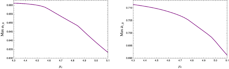
Figure 14: Maximum $\bar{a}_{1,0}$ vs. $\mu_{c}$ for $\mu_{2}=(1.65)^{2}$ computed at $k_{\max}=12$ in 10D (left) and in 4D (right).

Albert, Henriksson, Rastelli, and Vichi studied spectrum assumptions in the pion model in Albert:2023bml . Motivated by the experimentally observed meson spectrum, they input as the two-lowest mass states a spin $1$ particle (the $\rho$-meson $m_{\rho}=770$ MeV/$c^{2}$) at $\mu_{1}=1$ and the $f_{2}$-meson ($1270$ MeV/$c^{2}$) with spin 2 at $\mu_{2}=(1270/770)^{2}\approx(1.65)^{2}$. They find a corner in the maximum of the $f_{2}$-meson coupling $\tilde{g}_{f_{2}}^{2}$ near $\mu_{c}=4.748$. This translates to a mass of $\sqrt{4.748}\,m_{\rho}\approx 1678$ MeV/$c^{2}$, remarkably close to that of the spin 3 $\rho_{3}$ meson whose mass is $1690$ MeV/$c^{2}$. Similarly, an SDPB spectrum calculation gives a few more of the next states near the leading QCD Regge trajectory, see Figure 1 of Albert:2023bml . Unlike our corner theories in Section 4.3, the QCD meson spectrum is not linear.

The results of Albert:2023bml inspired us to extend our plots beyond $\mu_{2}=2$ and to look carefully at the $\mu_{2}=(1.65)^{2}$ case as well. We find that the $\text{max}(\bar{a}_{1,0})$ vs. $\mu_{c}$ curves have hints of two corners at masses greater than $(2\mu_{c}-1)M_{\text{gap}}^{2}$. For $\mu_{2}=(1.65)^{2}$, these “corners” are located at $\mu_{c}\approx 4.56$ and $\mu_{c}\approx 4.85$, neither of which match the pion model’s particularly well. Of course, this analysis is in 10D and with spins that are shifted by one compared with those of QCD. Re-analyzing the bounds in $D=4$, shown on the right hand side of Figure 14, the first corner is roughly at $\mu_{c}=4.77$, nearly matching the QCD spectrum! The other, more prominent corner moves to higher values, approximately $\mu_{c}=4.97$.

To compare more directly, we also plot the maximum of $|\bar{g}_{1}|^{2}$, the coupling to the vector state at $\mu_{2}=(1.65)^{2}$, in Figure 15. There is a clear corner for $\mu_{c}\approx 4.770$ (for $k_{\max}=16$). (We do not see any features in the $\text{max}(|\bar{g}_{1}|^{2})$ curve associated with the $\mu_{c}\approx 4.97$ corner of the Figure 14.) The quantity $|\bar{g}_{1}|^{2}$ is analogous to the coupling $\tilde{g}_{f_{2}}^{2}$ of the spin-two $f_{2}$ state of the pion model, shown in Figures 5 and 6 of Albert:2023bml . We use the same range of $\mu_{c}$ as the zoomed-in Figure 6 from Albert:2023bml . At $n_{\max}=17$ (their equivalent of $k_{\max}$), the corner in the pion bootstrap appears to be at $\mu_{c}\approx 4.747$, while for our bootstrap the $k_{\max}=16$ corner is closer to $4.770$. While not exact, the agreement is surprising for two ostensibly unrelated problems. The values of the maximal couplings near the corner, though, are not clearly directly related. This discrepancy is not unexpected since we are studying different models.

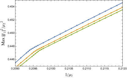
Figure 15: Maximum coupling, $|\bar{g}_{1}|^{2}$, for the vector at $\mu_{2}=(1.65)^{2}$ vs. $1/\mu_{c}$ computed at $k_{\max}=12$, $14$, and $16$ in 4D. The horizontal axis matches Figure 6 of Albert:2023bml for direct comparison, and we find a corner at $\mu_{c}$ within $\sim 0.02$ of theirs. We normalize $|\bar{g}_{1}|^{2}$ by $\mu_{2}^{2}$ to remove differences in definition from $\tilde{g}_{f_{2}}$ in Albert:2023bml .

5 Regge Bounds

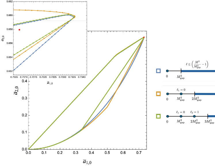
Figure 16: Outer bounds on the $k_{\max}=12~{}~{}(\bar{a}_{1,0},\bar{a}_{2,0})$ region with the Regge maximal spin requirement (blue), the scalar input at the mass gap with $\mu_{c}=2$ (orange), and the scalar at the mass gap and vector at $\mu_{2}=2$ input with $\mu_{c}=3$.

Imposing Regge-bounds, such as (4.2), together with the S-matrix bootstrap constraints has been pursued for both the closed and open string in Haring:2023zwu . Let us compare the spectrum restrictions resulting from imposing Regge slope 1 versus the single-state input at the mass gap $\mu_{c}=2$:

$$\begin{array}[]{lcl}\text{Regge:}~{}~{}\ell\leq\left(\frac{M^{2}}{M_{\text{gap}}^{2}}-1\right)&~{}\text{vs.}{}{}{}{}{}{}&\raisebox{-14.22636pt}{\includegraphics[width=142.26378pt]{Figures/SingleMassInput.pdf}}\\[7.11317pt] \text{1.~{}A state at the mass gap}&&\text{1.~{}At the mass gap, couplings }\\ \text{must be a scalar:}&&\text{of states with }\ell_{1}\leq 0~{}\text{are suppressed}\\ M^{2}=M_{\text{gap}}^{2}\implies\ell=0&&M^{2}=M_{\text{gap}}^{2}\implies\ell_{1}=0\\[7.11317pt] \text{2.~{}Scalars allowed }&&\text{2.~{}No states allowed }\\ \text{for $M_{\text{gap}}^{2}\leq M^{2}<2M_{\text{gap}}^{2}$}&&\text{for $M_{\text{gap}}^{2}<M^{2}<2M_{\text{gap}}^{2}$}\\[7.11317pt] \text{3.~{}Spin of states with $M^{2}\geq 2M_{\text{gap}}^{2}$}&&\text{3.~{}Spin of states with $M^{2}\geq 2M_{\text{gap}}^{2}$}\\ \text{restricted by Regge}&&\text{unrestricted}\end{array}$$ (5.1)

A priori, the bounds on Wilson coefficients resulting from these two different sets of constraints do not obviously have anything to do with each other. Surprisingly, we find that they are largely identical. This is illustrated in Figure 16, which for comparison also includes the bounds from inputting both the scalar state at the mass gap $M_{\text{gap}}^{2}$ and the vector at $2M_{\text{gap}}^{2}$.

It is surprising that what we consider a rather mild, low-spectrum constraint — a scalar at $M_{\text{gap}}^{2}$ and the string-inspired gap to the next state — yields essentially the same constraints on the $\bar{a}_{k,q}$ as the imposing the linear Regge behavior at all orders (up to the maximum spin considered for the numerical implementation) of the spectrum.

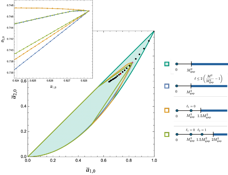
Figure 17: Outer bounds on the $k_{\max}=12~{}~{}(\bar{a}_{1,0},\bar{a}_{2,0})$ region with the Regge slope $\gamma=2$ maximal spin requirement (blue), the scalar input at the mass gap with $\mu_{c}=3/2$ (orange), and the scalar at the mass gap and vector at $\mu_{2}=3/2$ input with $\mu_{c}=2$. The black points indicate the locations of the tip of the allowed region for the “corner theories” parameterized by the first gap parameter $\mu_{2}$ (see Section 4.3). The brown dot is the case with $\mu_{2}=3/2$, and as shown it is right at the tip of the allowed region.

By considering different values of $\mu_{2}$, we found corners in the bounds corresponding to a 1-parameter family of models with linear trajectories $M^{2}_{\ell}=(\mu_{2}-1)\ell+1$. We can extend the analysis to compare the bounds from

$$\text{Regge:}~{}~{}\ell\leq\frac{1}{\mu_{2}-1}\left(\frac{M^{2}}{M_{\text{gap}}^{2}}-1\right)$$ (5.2)

to bounds obtained with the spectrum input

     and      (5.3)

The result for $\mu_{2}=1.5$ is shown in Figure 17. These bounds again give very similar constraints and they all have a sharp corner. This corner is where we expect to find the models with linear Regge trajectories.

In Section 4, we discussed how imposing the Regge bound can help give a cleaner SDPB spectrum. We have also tested how the combined constraints of Regge plus lowest mass state coupling input affect the bounds; details are given in Appendix B. In short, the outcome is that for the single state input with the scalar coupling fixed at the string-value, we get significantly smaller islands around the Veneziano amplitude when the Regge slope conditions are imposed. This is shown in Figure 21. However, for the two-state input, there is hardly any difference between the islands found from fixing the couplings of both the scalar and the vector to their string values versus those with the Regge slope condition added.

6 Discussion

We have shown that basic, low-energy input to maximally supersymmetric YM EFT generates novel, physically interesting features in the space of Wilson coefficients consistent with a local, unitary UV theory. We found that when there is a single state at bottom of the massive spectrum, it has to be a scalar. When we enforce the existence of a scalar at the mass gap $M_{\text{gap}}^{2}$, a vector at $\mu_{2}M_{\text{gap}}^{2}$, and no other states until a cutoff scale $\mu_{c}M_{\text{gap}}^{2}$, the maximal values of the $\bar{a}_{1,0}$ Wilson coefficient remains almost exactly the same until $\mu_{c}\approx 2\mu_{2}-1$, at which point it begins falling off rapidly. The dramatic change in behavior suggests the existence of an amplitude with a contribution from a spin two state at $\mu_{3}M_{\text{gap}}^{2}=(2\mu_{2}-1)M_{\text{gap}}^{2}$. This would correspond to a theory with a linear Regge trajectory.

If, instead of explicitly requiring the vector at $\mu_{2}M_{\text{gap}}^{2}$, we require that the scalar at $M_{\text{gap}}^{2}$ has a coupling to the massless states equal to that known from the Veneziano amplitude, then the maximal size of the second mass scale was found to be $\mu_{2}=2$. Assuming there are no states until $2M_{\text{gap}}^{2}$, the allowed region of Wilson coefficients shrinks to a small island. As more constraints are included from the derivative expansion, the islands were found to shrink in size, indicating that perhaps the only allowed point corresponds to the Veneziano amplitude in the $k_{\max}\rightarrow\infty$ limit. If the island did indeed shrink all the way, that would mean that to bootstrap Veneziano, one only needs two pieces of low-energy information:

1. that there is only one state at the lowest mass and it contributes via a pole exchange to the 4-point amplitude (the bootstrap then requires it must be a scalar),

2. the ratio, $|\bar{g}_{0}|^{2}=|g_{0}|^{2}/a_{0,0}$, between the massive scalar’s coupling to the massless external states and the ${\rm tr}F^{4}$ Wilson coefficient $a_{0,0}$.

In a practical scenario, these two inputs might necessarily become three because it would likely be difficult to determine $|\bar{g}_{0}|^{2}$ without measuring both $g_{0}$ and $a_{0,0}$ individually. It is still surprising, though, how little information is needed to bootstrap the Veneziano amplitude. It would be interesting to understand to what extent this is a consequence of supersymmetry and/or crossing.

Consider now what happens when we fix $|\bar{g}_{0}|^{2}$ to a something different from the string value. There are two qualitatively different cases to discuss, depending on whether $|\bar{g}_{0}|^{2}$ is greater or smaller than 1/2. Starting with the former, we find that the maximum allowed value of $|\bar{g}_{0}|^{2}$ is $(777-1120\log(2))=0.675158$, which occurs for the Infinite Spin Tower and requires the cutoff to be taken all the way down to the mass gap, $\mu_{c}=1$. The Single Scalar Exchange model (SSE, Section 2.5) has $|\bar{g}_{0}|^{2}=1/2$ and cutoff $\mu_{c}\rightarrow\infty$. Any value of $|\bar{g}_{0}|^{2}$ between these extremes, i.e. $1/2<|\bar{g}_{0}|^{2}\leq 0.675158$, will bootstrap the cutoff $\mu_{c}$ to a maximum allowed value between 1 and $\infty$. The resulting bounds are expected to be islands around the black points in Figure 17. These are the models with linear Regge slopes $1/(\text{max}(\mu_{c})-1)$ found as the corner theories in Section 4.3. It would be interesting to understand if these models have realizations as generalized versions of the Veneziano amplitude, as explored in for example Cheung:2022mkw ; Cheung:2023adk ; Cheung:2023uwn . If they exist, such new amplitudes would presumably have to interpolate between the SSE amplitude, the Veneziano amplitude, and the Infinite Spin Tower.

To actually compute this family of islands, one needs a very precise determination of the cutoff scale $\mu_{c}$ for a given value of $|\bar{g}_{0}|^{2}$; since the islands are going to be small, slightly different values of $\mu_{c}$ can give mutually excluding islands. For any finite value of $k_{\max}$, one can determine the maximum allowed value of $\mu_{c}$, but one would then need to extrapolate that to $k_{\max}\rightarrow\infty$. Alternatively, one can specify the cutoff $\mu_{c}$ and seek to bootstrap the value of $|\bar{g}_{0}|^{2}$ by a maximization principle.

From a theoretical perspective there is no reason to necessarily favor coupling input over input of the cutoff mass. Imagine doing a bootstrap like this in an context where the input comes from actual experimental data. One may then view the coupling choice as more well-motivated than the gap input because in an experimental situation that directly produces a high energy particle, we would be able to determine both the spin and coupling of that state. On the other hand, it would be impossible to experimentally determine the exact gap to the next state without having enough energy to produce it, at which point, the spin and coupling of that state could be used as bootstrap input. However, an experiment would not give us an exact value for any measurement, so the ratio $|\bar{g}_{0}|^{2}$ would be determined with some error. The bootstrapped maximal $\mu_{c}$ value would then give the approximate scale at which new physics must appear. To get a reasonable “island” in such a scenario, one would have to compute islands for a selection of values of $|\bar{g}_{0}|^{2}$ within the experimental bounds and their corresponding largest cutoff scale. The full allowed region of Wilson coefficients would then be obtained from smearing of these islands. This smeared region would likely not shrink to a single point with increasing $k_{\text{max}}$, but would still be far more constraining than any naive bound.

Consider now the range of couplings $0\leq|\bar{g}_{0}|^{2}\leq 1/2$. In this case, there is no maximal cutoff mass $\mu_{c}$. Similarly to the case of SSE with $|\bar{g}_{0}|^{2}=1/2$, we only expect islands in the $\mu_{c}\rightarrow\infty$ limit. Models with $0\leq|\bar{g}_{0}|^{2}\leq 1/2$ can be obtained as linear combinations of SSE amplitudes with different choices of $m^{2}$, for example (with $M_{\text{gap}}=1$ for simplicity)

$$\lambda A_{1}^{\text{SSE}}+(1-\lambda)A_{m^{2}}^{\text{SSE}}\,.$$ (6.1)

For this amplitude, $|g_{0}|^{2}=\lambda/2$ because when $m^{2}>1$ its only contribution is from the $A_{1}^{\text{SSE}}$ part of the amplitude. The coefficient $a_{0,0}$, on the other hand, is given by $a_{0,0}=(\lambda+(1-\lambda)/m^{2})$, and so the ratio becomes

$$|\bar{g}_{0}|^{2}=\frac{\lambda}{2(\lambda+(1-\lambda)/m^{2})}\,.$$ (6.2)

By then setting $m^{2}=r/\lambda$, we find that in the limit of $\lambda\rightarrow 0$ and $r$ fixed,

$$\lim_{\lambda\rightarrow 0}|\bar{g}_{0}|^{2}=\frac{r}{2r+2}\,.$$ (6.3)

Therefore, $0<|\bar{g}_{0}|^{2}<1/2$ is allowed and gives examples of islands in a limiting sense.

Returning to the bootstrap of the Veneziano amplitude, one potential path to stronger bounds is through the fact that, in the Regge limit with fixed $u<0$, the Veneziano amplitude (1.3) actually scales with large $|s|$ as

$$\lim_{|s|\rightarrow\infty}\frac{A^{\text{str}}(s,u)}{s}\sim s^{u}\rightarrow 0\,.$$ (6.4)

This is one power of $s$ stronger than we assume with the Froissart bound that $A(s,u)/s^{2}\rightarrow 0$. Therefore, one could restrict to amplitudes that have this improved Regge behavior and derive additional null constraints that correspond to the fact that $a_{k,k+1}=0$ for all $k\geq-1$. This rules out, for example, the SSE amplitude, so it could improve our ability to corner and isolate the string. The implementation of these null constraints is discussed in AKRboot using techniques developed in Caron-Huot:2021rmr .

The type of bounds computed in this paper are so-called “dual” bootstrap bounds. Any point outside of our bounds does not have a unitary UV completion (with the specified assumptions), but points within our bounds may or may not have them. An important aspect of the bootstrap program not considered in this work is the “primal” formulation of the S-matrix bootstrap, which has been studied for permutation symmetric scalars, pions, photons, and gravitons Guerrieri:2020bto ; Guerrieri:2021ivu ; Chen:2022nym ; Haring:2022sdp ; Haring:2023zwu ; Li:2023qzs . In the primal version of the bootstrap, unitarity is imposed numerically on an ansatz that manifestly satisfies both locality and crossing symmetry, and points within their bounds necessarily have a unitary UV complete amplitude, but points outside could as well. The primal bootstrap has the advantage of being clearly applicable beyond the strict perturbative limit. Further, as shown in Haring:2023zwu ; Li:2023qzs , there can be reasonably good agreement between the dual and primal bounds. It would be interesting to know whether the primal type bounds could rule-in parameter space such that we can test if the scalar-input islands somehow do not continue to shrink to include the string alone.

Finally, the fact that low-energy input leads to important new features of the space of allowed Wilson coefficients in both the pion and $\mathcal{N}=4$ SYM models suggests that such features might also appear in less mathematically similar bootstrap problems. If the appearance of novel features is generic, one might hope to eventually apply these principles to more phenomenologically relevant models as well.

Appendix A Implementation as an SDP

A.1 Null Constraints

There are two sets of null constraints: the $\mathcal{X}$-constraints are due to the basic SUSY crossing condition $a_{k,q}-a_{k,k-q}=0$, and the $\mathcal{Y}$-constraints come from reconciliation of dispersive representations of the $a_{k,q}$ derived for fixed $u$ and fixed $t$. These two sets of conditions impose constraints on the spectral density and they were derived in detail in Berman:2023jys . They are

$$\begin{split}&\forall~{}k,q\!:~{}~{}~{}\sum_{\ell=0}\int_{0}^{1}dx\,p_{\ell}(x)\,\mathcal{X}^{\ell,x}_{k,q}=0~{}~{}~{}\text{with}~{}~{}~{}\mathcal{X}^{\ell,x}_{k,q}=x^{k}\big{[}v_{\ell,q}-v_{\ell,k-q}\big{]}\,\\ &\forall~{}k,q\!:~{}~{}~{}\sum_{\ell}\int_{0}^{1}dx\,p_{\ell}(x)\,\mathcal{Y}^{\ell,x}_{k,q}=0\\ &\text{with}~{}~{}~{}\mathcal{Y}^{\ell,x}_{k,q}=x^{k}\left[v_{\ell,q}-(-1)^{\ell}\sum_{q^{\prime}=0}^{k}(-1)^{q^{\prime}}v_{\ell,q^{\prime}}\left(\binom{q^{\prime}}{k-q}+\binom{q^{\prime}}{q}\right)\right]\,,\end{split}$$ (A.1)

where

$$x\equiv\frac{M_{\text{gap}}^{2}}{M^{2}}=y^{-1}\quad\text{and}\quad p_{\ell}(x)\equiv x\rho_{\ell}\big{(}M_{\textrm{gap}}^{2}/x\big{)}=y^{2}f_{\ell}(y)\,.$$ (A.2)

We can rewrite these in terms of $y$ and $f_{\ell}(y)$ to match the notation here by simply making a change of variables from $x\rightarrow y$. Doing this variable replacement takes

$$x^{k}p_{\ell}(x)dx=y^{-k}(y^{-3}\rho(M_{\text{gap}}^{2}y))dy=y^{-k}f_{\ell}(y)dy\,.$$ (A.3)

Thus, we find that in terms of $y$ and $f_{\ell}(y)$, the null constraints become

$$\begin{split}&\forall~{}k,q\!:~{}~{}~{}\sum_{\ell=0}\int_{1}^{\infty}dy\,f_{\ell}(y)\,\mathcal{X}^{\ell,y}_{k,q}=0~{}~{}~{}\text{with}~{}~{}~{}\mathcal{X}^{\ell,y}_{k,q}=y^{-k}\big{[}v_{\ell,q}-v_{\ell,k-q}\big{]}\,\\ &\forall~{}k,q\!:~{}~{}~{}\sum_{\ell}\int_{1}^{\infty}dy\,f_{\ell}(y)\,\mathcal{Y}^{\ell,y}_{k,q}=0\\ &\text{with}~{}~{}~{}\mathcal{Y}^{\ell,y}_{k,q}=y^{-k}\left[v_{\ell,q}-(-1)^{\ell}\sum_{q^{\prime}=0}^{k}(-1)^{q^{\prime}}v_{\ell,q^{\prime}}\left(\binom{q^{\prime}}{k-q}+\binom{q^{\prime}}{q}\right)\right]\,.\end{split}$$ (A.4)

A.2 Explicit States

For the practical implementation in SDPB, it is convenient to set $M_{\text{gap}}=1$. Recall that the dispersive representation (2.8) is

$$a_{k,q}=\sum_{\ell=0}^{\infty}\int_{1}^{\infty}dy\,y^{-k}f_{\ell}(y)\,v_{\ell,q}\,.$$ (A.5)

Consider the case of a spin-0 state at the mass gap ($y=1$) and a spin 1 state at $y=\mu_{2}$. The simple poles correspond to delta functions in the spectral density, so with the definition of $f_{\ell}(y)$ above equation (2.9), we have

$$f_{\ell}(y)=\delta(y-1)\delta_{\ell,0}|g_{0}|^{2}+\delta(y-\mu_{2})\delta_{\ell,1}|g_{1}|^{2}\frac{1}{\mu_{2}^{3}}+f^{(\mu_{c})}_{\ell}(y)\,,$$ (A.6)

where $f^{(\mu_{c})}_{\ell}(y)$ only has support for $y\geq\mu_{c}$. From this, one obtains eq. (2.20).

The derivation of the null constraints using the full $f_{\ell}(y)$ gives exactly the same results as without spectral input. We denote these crossing constraints jointly as “null” in the following. Using the “bracket-notation” (2.9) the general vertex representation (2.25) is of the form

$$\vec{V}=\big{\langle}\vec{E}\big{\rangle}_{1}\,,$$ (A.7)

where $\vec{V}$ and $\vec{E}_{\ell,y}$ are described briefly in Section 2.6; more explicit expressions can be found in equation (4.2) in Berman:2023jys . The precise specification of (A.7) depends on which quantity we wish to extremize. It is useful to note, for example, that it follows from (A.6) that

$$\big{\langle}\vec{E}\big{\rangle}_{1}=|g_{0}|^{2}\vec{E}_{0,1}+|g_{1}|^{2}\frac{1}{\mu_{2}^{3}}\vec{E}_{1,\mu_{2}}+\big{\langle}\vec{E}\big{\rangle}_{\mu_{c}}\,.$$ (A.8)

This is the key ingredient in the following.

A.3 Optimization problem: maximizing $a_{k,q}$

Define

$$\vec{V}=\begin{pmatrix}a_{0,0}\\ a_{k,q}\\[5.69054pt] \langle\,\overrightarrow{\text{null}}\,\rangle_{1}\end{pmatrix}~{}~{}~{}\text{and}~{}~{}~{}\vec{E}_{\ell,y}=\begin{pmatrix}1\\ y^{-k}v_{\ell,q}\\[5.69054pt] \overrightarrow{\text{null}}_{\ell,y}\end{pmatrix}\,,$$ (A.9)

where $\langle\,\overrightarrow{\text{null}}\,\rangle_{1}$ indicates all the null constraints, which may including also conditions such as $a_{k^{\prime},q^{\prime}}=Ra_{0,0}$ that sets the question to: what are the extremal values of $a_{k,q}/a_{0,0}$ when $a_{k^{\prime},q^{\prime}}/a_{0,0}$ is fixed to be $R$.

Now let

$$\vec{\alpha}=(A,-1,\vec{\beta})\,.$$ (A.10)

With the vanishing of the null constraints, it is clear that $\vec{\alpha}\cdot\vec{V}=Aa_{0,0}-a_{k,q}$. Hence, if we assume that

$$\begin{split}&\vec{\alpha}\cdot\vec{E}_{0,1}\geq 0\,,~{}~{}~{}~{}\vec{\alpha}\cdot\vec{E}_{1,\mu_{2}}\geq 0\,,~{}~{}~{}~{}\\ &\vec{\alpha}\cdot\vec{E}_{\ell,y}\geq 0~{}~{}~{}~{}\text{for all }\ell=0,1,\ldots,\ell_{\text{max}}~{}~{}~{}\text{and}~{}~{}~{}y\geq\mu_{c}\,,\end{split}$$ (A.11)

then $\vec{\alpha}\cdot\vec{V}=\big{\langle}\vec{\alpha}\cdot\vec{E}\big{\rangle}_{1}\geq 0$ implies that on the vanishing of the null constraints

$$Aa_{0,0}-a_{k,q}\geq 0~{}~{}~{}~{}\implies~{}~{}~{}~{}A\geq\frac{a_{k,q}}{a_{0,0}}\,,$$ (A.12)

so that minimizing $A$ is maximizing $a_{k,q}/a_{0,0}$. In SDPB, the conditions $\vec{\alpha}\cdot\vec{E}_{0,1}\geq 0$ and $\vec{\alpha}\cdot\vec{E}_{1,\mu_{2}}\geq 0$ simply mean that we allow for scalar or vector states, respectively, at $y=1$ and $y=\mu_{2}$. Leaving out one or both of these conditions mean that we disallow all states at the respective masses.

It is useful to reformulate the problem as follows. Write

$$\vec{V}=a_{0,0}\vec{v}_{1}-a_{k,q}\vec{v}_{O}+\vec{V}_{\text{null}}\,,~{}~{}~{}~{}\vec{V}_{\text{null}}=\begin{pmatrix}0\\ 0\\[5.69054pt] \langle\,\overrightarrow{\text{null}}\,\rangle_{1}\end{pmatrix}$$ (A.13)

for $\vec{v}_{1}=(1,0,0,\dots)$ and $\vec{v}_{O}=(0,-1,0,\dots)$. The vector $\vec{v}_{1}$ identifies the quantity we optimize in $\vec{\alpha}$, i.e. $A=\vec{\alpha}\cdot\vec{v}_{1}$ whereas the objective vector $\vec{v}_{O}$ ensures the proper normalization of the “objective” of our optimization by having

$$\vec{\alpha}\cdot\vec{v}_{O}=1\,.$$ (A.14)

Next, consider optimization of the couplings $|g_{0}|^{2}$ and $|g_{1}|^{2}$.

A.4 Optimization problem: bounding couplings

In this Appendix, we describe two methods for optimizing couplings.

Bounding Couplings by Choosing Objective Vectors

The approach described here was developed in Albert:2022oes . Define

$$\vec{V}=\begin{pmatrix}a_{0,0}\\[5.69054pt] \langle\,\overrightarrow{\text{null}}\,\rangle_{1}\end{pmatrix}~{}~{}~{}\text{and}~{}~{}~{}\vec{E}_{\ell,y}=\begin{pmatrix}1\\[5.69054pt] \overrightarrow{\text{null}}_{\ell,y}\end{pmatrix}$$ (A.15)

i.e.

$$\vec{V}=a_{0,0}\vec{v}_{1}+\vec{V}_{\text{null}}\,,~{}~{}~{}~{}\text{with}~{}~{}~{}\vec{V}_{\text{null}}=\begin{pmatrix}0\\[5.69054pt] \langle\,\overrightarrow{\text{null}}\,\rangle_{1}\end{pmatrix}$$ (A.16)

This time we pick $\vec{\alpha}=(A,\vec{\beta})$. We now describe how to use $\vec{V}=\big{\langle}\vec{E}\big{\rangle}_{1}$ to maximize $|g_{0}|^{2}$. Then we show how a similar approach is used to extremize $|g_{1}|^{2}$.

• Maximize $|g_{0}|^{2}$.

  With the help of (A.8), we can write $\vec{V}=\big{\langle}\vec{E}\big{\rangle}_{1}$ as

  $$a_{0,0}\vec{v}_{1}-|g_{0}|^{2}\vec{E}_{0,1}+\vec{V}_{\text{null}}=|g_{1}|^{2}\frac{1}{\mu_{2}^{3}}\vec{E}_{1,\mu_{2}}+\big{\langle}\vec{E}\big{\rangle}_{\mu_{c}}\,.$$ (A.17)

  This can be viewed as an optimization problem like (A.13) with objective $|g_{0}|^{2}$ and objective vector $\vec{v}_{O}=\vec{E}_{0,1}$. The normalization condition (A.14) then says that we need to have

  $$\vec{\alpha}\cdot\vec{E}_{0,1}=1\,.$$ (A.18)

  Using that, and imposing the null constraints, we then find that dotting $\vec{\alpha}$ into (A.17) gives

  $$a_{0,0}A-|g_{0}|^{2}=|g_{1}|^{2}\frac{1}{\mu_{1}^{3}}\,\vec{\alpha}\cdot\vec{E}_{1,\mu_{1}}+\big{\langle}\vec{\alpha}\cdot\vec{E}\big{\rangle}_{\mu_{c}}\,$$ (A.19)

  so that if we impose

  $$\begin{split}&\vec{\alpha}\cdot\vec{E}_{1,\mu_{2}}\geq 0\,,~{}~{}~{}~{}\\ &\vec{\alpha}\cdot\vec{E}_{\ell,y}\geq 0~{}~{}~{}~{}\text{for all }\ell=0,1,\ldots,\ell_{\text{max}}~{}~{}~{}\text{and}~{}~{}~{}y\geq\mu_{c}\,,\end{split}$$ (A.20)

  then we get

  $$a_{0,0}A-|g_{0}|^{2}\geq 0~{}~{}~{}\implies~{}~{}~{}A\geq\frac{|g_{0}|^{2}}{a_{0,0}}$$ (A.21)

  i.e. minimizing $A$ maximizes $|g_{0}|^{2}/a_{0,0}$.

• Maximize $|g_{1}|^{2}$.

  Using (A.8), we now write $\vec{V}=\big{\langle}\vec{E}\big{\rangle}_{1}$ as

  $$a_{0,0}\vec{v}_{1}-|g_{1}|^{2}\frac{1}{\mu_{2}^{3}}\vec{E}_{1,\mu_{2}}+\vec{V}_{\text{null}}=|g_{0}|^{2}\vec{E}_{0,1}+\big{\langle}\vec{E}\big{\rangle}_{\mu_{c}}\,.$$ (A.22)

  To extremize $|g_{1}|^{2}$, we choose the objective vector $\vec{v}_{O}=\frac{1}{\mu_{2}^{3}}\vec{E}_{1,\mu_{2}}$ and the normalization condition (A.14) then becomes

  $$\mu_{2}^{-3}\,\vec{\alpha}\cdot\vec{E}_{1,\mu_{2}}=1\,.$$ (A.23)

  Dotting $\vec{\alpha}$ into (A.22) and imposing the null constraints then gives

  $$a_{0,0}A-|g_{1}|^{2}\geq 0$$ (A.24)

  assuming that

  $$\begin{split}&\vec{\alpha}\cdot\vec{E}_{0,1}\geq 0\,,~{}~{}~{}~{}\\ &\vec{\alpha}\cdot\vec{E}_{\ell,y}\geq 0~{}~{}~{}~{}\text{for all }\ell=0,1,\ldots,\ell_{\text{max}}~{}~{}~{}\text{and}~{}~{}~{}y\geq\mu_{c}\,.\end{split}$$ (A.25)

  As in previous cases, this lets us find the maximum of $|g_{1}|^{2}/a_{0,0}$ by minimizing $A$.

Bounding Couplings by Solving Null Constraints

The above approach allows us to bound couplings $|g_{\ell,\mu}|^{2}$ of the massive exchanged particles to the massless particles relative to $a_{0,0}$. However, it does not allow to fix $|\bar{g}_{\ell,\mu}|^{2}=|g_{\ell,\mu}|^{2}/a_{0,0}$ to a specific value. To do so, we use a different method which is to use the null constraints to derive dispersive representations for the couplings $|g_{\ell,\mu}|^{2}$ that we want to fix.

As a simple example of this, suppose we want to fix the coupling $|g_{0}|^{2}$ in (3.3) to a specific value. Since $|g_{0}|^{2}$ enters the null condition $a_{1,0}=a_{1,1}$, we can use that to solve for $|g_{0}|^{2}$. Start with

$$0=a_{1,0}-a_{1,1}=|g_{0}|^{2}(v_{0,1}-v_{0,0})+\langle y^{-1}(v_{l,1}-v_{l,0})\rangle_{\mu_{c}}$$ (A.26)

where we used that the high energy average is a linear operation. Using that $v_{l,q}=0$ for $q>\ell$ and $v_{0,0}=1$, we solve for $|g_{0}|^{2}$ find

$$|g_{0}|^{2}=\langle y^{-1}(v_{l,1}-v_{l,0})\rangle_{\mu_{c}}.$$ (A.27)

Using this dispersive representation, we can fixed $|\bar{g}_{0}|$ to a specific value $R$ in the numerical bootstrap by making $|g_{0}|^{2}-Ra_{0,0}$ a null constraint in our vector $\vec{V}$. The dispersive representation (A.27) determines the corresponding entry in the $\vec{E}_{\ell,y}$ vectors.

To fix more couplings we can use more null conditions. For example, if we want to fix both $|\bar{g}_{0}|^{2}$ and $|\bar{g}_{1}|^{2}$ as discussed in the maintext, we can use $a_{1,0}=a_{1,1}$ along with $0=a_{3,1}-a_{3,2}$ (that is the lowest-$k$ null relation to which $|g_{0}|^{2}$ does not contribute). Then, we find

$$0 =a_{1,0}-a_{1,1}=|g_{0}|^{2}(v_{0,1}-v_{0,0})+\frac{|g_{1}|^{2}}{\mu_{2}^{4}}(v_{1,1}-v_{1,0})+\langle y^{-1}(v_{l,1}-v_{l,0})\rangle_{\mu_{c}}$$ (A.28)

$$0 =a_{3,1}-a_{3,2}=|g_{0}|^{2}(v_{0,1}-v_{0,2})+\frac{|g_{1}|^{2}}{\mu_{2}^{6}}(v_{1,1}-v_{1,2})+\langle y^{-3}(v_{l,1}-v_{l,2})\rangle_{\mu_{c}}\,.$$ (A.29)

Using the fact that $v_{l,q}=0$ for $q>l$ to simplify these expressions, along with $v_{1,1}=2$, we solve the linear system that can be solved to give $|g_{0}|^{2}$ and $|g_{1}|^{2}$ in terms of their high energy integrals:

$$|g_{0}|^{2} =\frac{\mu_{2}^{2}}{2}\langle y^{-3}(v_{l,2}-v_{l,1})\rangle_{\mu_{c}}+\langle y^{-1}(v_{l,1}-v_{l,0})\rangle_{\mu_{c}}$$ (A.30)

$$|g_{1}|^{2} =\frac{\mu_{2}^{6}}{2}\langle y^{-3}(v_{l,2}-v_{l,1})\rangle_{\mu_{c}}\,.$$ (A.31)

In principle, we could use a null constraint of any order to solve for a coefficient. However, to keep track of $k_{\max}$ properly, we restrict ourselves to using only null constraints up to those with $k=k_{\max}$. To have access to the null constraint $0=a_{3,1}-a_{3,2}$ we need to take $k_{\max}\geq 3$ and the maximal number of couplings we can fix depends on $k_{\max}$.

When we solve for couplings using null relations, we are no longer strictly enforcing their positivity. Hence, we only use this approach when we either fix or extremize a coupling that is solved for by the null conditions; otherwise, we risk allowing non-unitary theories where these couplings are negative. It is important to note that when we use SDPB to minimize a coupling $\bar{g}_{\ell,\mu_{n}}$, it may give a negative value, so we enforce positivity by hand, taking Min$|\bar{g}_{\ell,\mu_{n}}|^{2}=$ Max$(0,$ SDPB minimum$)$.

Figure 18: Left: The $\bar{a}_{1,0}$ and $\bar{a}_{2,0}$ with no spectral assumptions in teal and when the lowest massive states are assumed to be a scalar at the mass gap $M_{\text{gap}}^{2}$, a vector at $2M_{\text{gap}}^{2}$, and a further mass-gap to $3M_{\text{gap}}^{2}$ in purple. The purple region has a corner very close to the Veneziano amplitude (red dot). Right: Zoom-in around the corner of the purple region. For comparison is also shown in light purple the allowed region when we only input a spin 0 particle at $M_{\text{gap}}^{2}$ and a further mass gap to $2M_{\text{gap}}^{2}$. The bounds for these regions were computed with $k_{\text{max}}=10$.

Appendix B Multi-State Bootstrap of Veneziano

In this appendix, we compare the corner and island bootstrap of the Veneziano amplitude for two different types of low energy assumptions: (1) the single state input from Section 3 with a a scalar at $M_{\text{gap}}^{2}$ and no states until the cutoff at $2M_{\text{gap}}^{2}$ versus (2) inputting the two lowest mass states: a scalar at $M_{\text{gap}}^{2}$, a vector at $2M_{\text{gap}}^{2}$ and no other states until $3M_{\text{gap}}^{2}$ (which is the “corner” value for the cutoff discussed in Section 4.1).

B.1 Corners

For the two state input discussed above, we have

$$a_{k,q}=|g_{0}|^{2}v_{0,q}+\frac{|g_{1}|^{2}}{2^{k+3}}v_{1,q}+\Big{\langle}y^{-k}v_{\ell,q}\Big{\rangle}_{3}\,.$$ (B.1)

With this input, the allowed region of the $(\bar{a}_{1,0},\bar{a}_{2,0})$-plane is shown in Figure 18 is somewhat smaller than that of just the single scalar input and still has the string amplitude at the corner. Most importantly, the corner near the string is, as shown on the right of Figure 18 quite a bit sharper than with just the single mass input.

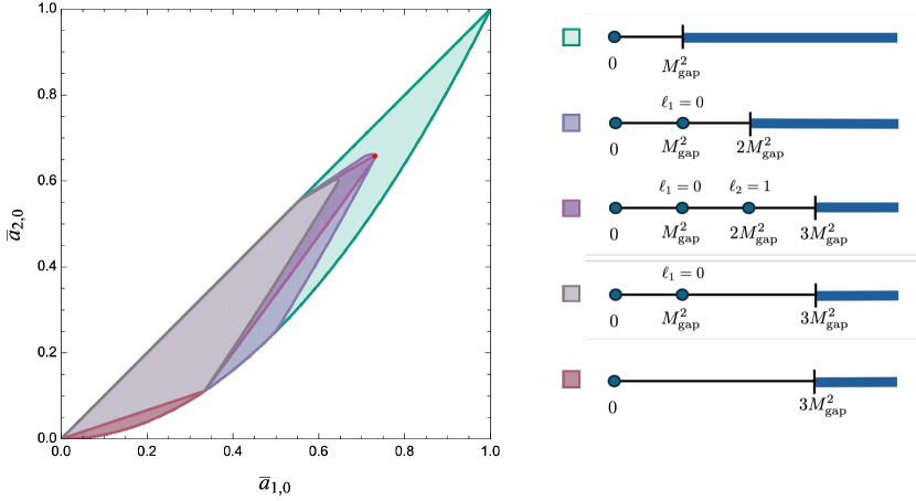
Figure 19: Allowed regions for listed spectrum assumptions at $k_{\max}=10$.

It is interesting to see how the regions are built up and which parts of them are sensitive to the various mass and spin inputs. In Figure 19, we show the allowed regions in the $(\bar{a}_{1,0},\bar{a}_{2,0})$-plane for various different spectral assumptions. The red region shows the allowed region with no states allowed all the way to the cutoff at $3M_{\text{gap}}^{2}$. A large chunk of parameter space becomes allowed if we turn on the $g_{0}$ coupling, allowing for a scalar at $M_{\text{gap}}^{2}$. If we keep the cutoff at $3M_{\text{gap}}^{2}$, the region, shown in gray excludes the string (red dot), but when the cutoff is reduced to $2M_{\text{gap}}^{2}$, we get the blue-gray region that now includes the string. This is the region studied previously in Section 3.2 and shown in Figure 1. Next, we allow for a vector at $2M_{\text{gap}}$ we get the region shown in dark purple, for which the Veneziano amplitude is at the sharp corner.

The Next Corner. The cutoff $\mu_{c}=3$ was chosen as the value near the corner in the $\bar{a}_{1,0}$ maximum value. It is interesting to consider what happens if we continued with further string-y input and take the existence of this spin two state as something “implied” by the bootstrap and then use it to find where the next state in the spectrum lives. We then have a dispersion relation of the form

$$a_{k,q}=|g_{0}|^{2}v_{0,q}+\frac{|g_{1}|^{2}}{2^{k+3}}v_{1,q}+\frac{|g_{2}|^{2}}{3^{k+3}}v_{2,q}+\Big{\langle}y^{-k}v_{\ell,q}\Big{\rangle}_{\mu_{c}}\,.$$ (B.2)

Figure 20 shows maximal $\bar{a}_{1,0}$ vs. the cutoff. The maximal values is almost exactly constant from $\mu_{c}=3$ to $\mu_{c}=4$ and then has a dramatic falloff, indicating the need for a new state at $4M_{\text{gap}}^{2}$. This is corroborated by the SDPB spectrum from Figure 11 which also indicated that there is a spin 2 state at $4M_{\text{gap}}^{2}$.

At $4M_{\text{gap}}^{2}$, we encounter another feature of the string spectrum: the first daughter trajectory. There is not just a spin three state at $M^{2}=4/\alpha^{\prime}$, but also a spin one state exchanged. The fact that a corner appears at (or near) $\mu_{4}=4$ does not tell us what spin the particle there should have, so we can turn to SDPB’s spectrum analysis to test for the states that live at the feature. As before, the extremal spectrum does not contain any daughter trajectories, so we do not see any purely bootstrap way to proceed along the string spectrum, at least for the values of $k_{\max}$ we can achieve. Additional assumptions, such as the Regge slope help a bit, but the spectrum is still not clean.

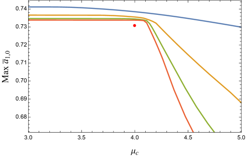
Figure 20: The maximal $\bar{a}_{1,0}$ vs. $\mu_{c}$ at $k_{\max}=4,6,8,10$ for the spectrum given by (B.2).

B.2 Islands

In Section 3.3, we showed that fixing $|\bar{g}_{0}|^{2}$, the coupling of the scalar at the mass gap, resulted in a maximal allowed cutoff mass $\mu_{c}M_{\text{gap}}^{2}$. A unitary theory must have new massive states at or below that maximum value. We found that when $|\bar{g}_{0}|^{2}$ was taken to be its string value, the maximum cutoff mass corresponded precisely to the mass at which the second string state appeared, namely as $2M_{\text{gap}}^{2}$. Fixing $\mu_{c}=2$, we found shrinking islands around the Veneziano amplitude Wilson coefficients.

To get stronger bounds we now impose stronger assumptions on the spectrum. Specifically, we input information about the state at $2M_{\text{gap}}^{2}$, as in the previous section.

We first consider a dispersion relation of the form

$$\bar{a}_{k,q}=\frac{v_{0,q}}{\zeta_{2}}+\frac{|g_{\ell_{2},2}|^{2}v_{\ell_{2},q}}{2^{k+3}\zeta_{2}}+\Big{\langle}y^{-k}v_{\ell,q}\Big{\rangle}_{\mu_{c}}\,,$$ (B.3)

where the spin $\ell_{2}$ of the state at $\mu_{2}=2$ and the cutoff $\mu_{c}>2$ are unfixed. We find that, by $k_{\max}=12$, there are no theories compatible with the bounds unless $\ell_{2}=1$, i.e. there has to be a vector at the state at $2M_{\text{gap}}^{2}$. With that vector assumed, any state with spin $\ell>1$ has a coupling that gets suppressed exponentially with $k_{\max}$, similar to what we saw in Section 3.1 for non-scalar states at the mass gap. The maximal coupling to a scalar state at $2M_{\text{gap}}^{2}$ decreases with $k_{\max}$, but it does not appear to approach zero as quickly as those for $\ell>1$, so there is not any clear a priori reason to rule it out.

Figure 21: Left: Bounds on the $k_{\max}=4,6,8,10,12$ $(\bar{a}_{1,0},\bar{a}_{2,0})$ allowed region with a scalar at the gap and a vector at $\mu_{2}=2$ with their string couplings along with a cutoff $\mu_{c}=3$. Right: Comparing the scalar-only island with smaller scalar with Regge slope, scalar and vector, and scalar and vector with Regge slope island at $k_{\max}=12$.

To proceed, we simply make the string-inspired choice to add in just the vector state with its coupling and as well as a gap to $\mu_{c}=3$. The dispersion relation for the Wilson coefficients is then

$$\bar{a}_{k,q}=\frac{v_{0,q}}{\zeta_{2}}+\frac{2v_{1,q}}{2^{k+3}\zeta_{2}}+\Big{\langle}y^{-k}v_{\ell,q}\Big{\rangle}_{3}\,,$$ (B.4)

using $|\bar{g}_{0}^{\text{str}}|^{2}=1/\zeta_{2}$ and $|\bar{g}_{1}^{\text{str}}|^{2}=2/\zeta_{2}$. The bootstrap then gives small shrinking islands around the Veneziano amplitude, as shown on the right of Figure 21. The size of these islands are considerably smaller than the those with only the single state input (e.g. Figure 2). A direct comparison of the $k_{\text{max}}=12$ islands for the single and double state input is given on the right of Figure 21. For further comparison, we also include in that plot the islands obtained with the same one- and two-state input but with the additional assumption of no states below the leading Regge trajectories (as discussed in Section 5.). This assumption has a significant effect on the single-scalar island, but results in hardly any change for the two-scalar island.

References

- (1) S. Caron-Huot and V. Van Duong, Extremal Effective Field Theories, 2011.02957.
- (2) N. Arkani-Hamed, T.-C. Huang and Y.-T. Huang, The EFT-Hedron, JHEP 05 (2021) 259 [2012.15849].
- (3) L.-Y. Chiang, Y.-t. Huang, W. Li, L. Rodina and H.-C. Weng, Into the EFThedron and UV constraints from IR consistency, JHEP 03 (2022) 063 [2105.02862].
- (4) J. Albert and L. Rastelli, Bootstrapping pions at large N, JHEP 08 (2022) 151 [2203.11950].
- (5) S. Caron-Huot, Y.-Z. Li, J. Parra-Martinez and D. Simmons-Duffin, Graviton partial waves and causality in higher dimensions, Phys. Rev. D 108 (2023) 026007 [2205.01495].
- (6) C. Fernandez, A. Pomarol, F. Riva and F. Sciotti, Cornering Large- QCD with Positivity Bounds, 2211.12488.
- (7) J. Albert and L. Rastelli, Bootstrapping Pions at Large . Part II: Background Gauge Fields and the Chiral Anomaly, 2307.01246.
- (8) L. Alberte, C. de Rham, S. Jaitly and A. J. Tolley, QED positivity bounds, Phys. Rev. D 103 (2021) 125020 [2012.05798].
- (9) J. Henriksson, B. McPeak, F. Russo and A. Vichi, Rigorous bounds on light-by-light scattering, JHEP 06 (2022) 158 [2107.13009].
- (10) S. D. Chowdhury, K. Ghosh, P. Haldar, P. Raman and A. Sinha, Crossing Symmetric Spinning S-matrix Bootstrap: EFT bounds, SciPost Phys. 13 (2022) 051 [2112.11755].
- (11) S. Caron-Huot, Y.-Z. Li, J. Parra-Martinez and D. Simmons-Duffin, Causality constraints on corrections to Einstein gravity, 2201.06602.
- (12) C. de Rham, L. Engelbrecht, L. Heisenberg and A. Lüscher, Positivity bounds in vector theories, JHEP 12 (2022) 086 [2208.12631].
- (13) T. Ma, A. Pomarol and F. Sciotti, Bootstrapping the chiral anomaly at large Nc, JHEP 11 (2023) 176 [2307.04729].
- (14) M. Carrillo González, C. de Rham, S. Jaitly, V. Pozsgay and A. Tokareva, Positivity-causality competition: a road to ultimate EFT consistency constraints, 2307.04784.
- (15) J. Berman, H. Elvang and A. Herderschee, Flattening of the EFT-hedron: supersymmetric positivity bounds and the search for string theory, JHEP 03 (2024) 021 [2310.10729].
- (16) L.-Y. Chiang, Y.-t. Huang and H.-C. Weng, Bootstrapping string theory EFT, JHEP 05 (2024) 289 [2310.10710].
- (17) J. Albert, J. Henriksson, L. Rastelli and A. Vichi, Bootstrapping mesons at large : Regge trajectory from spin-two maximization, 2312.15013.
- (18) K. Häring and A. Zhiboedov, The Stringy S-matrix Bootstrap: Maximal Spin and Superpolynomial Softness, 2311.13631.
- (19) G. Veneziano, Construction of a crossing - symmetric, Regge behaved amplitude for linearly rising trajectories, Nuovo Cim. A 57 (1968) 190.
- (20) E. Plahte, Symmetry properties of dual tree-graph n-point amplitudes, Nuovo Cim. A 66 (1970) 713.
- (21) S. Stieberger, Open & Closed vs. Pure Open String Disk Amplitudes, 0907.2211.
- (22) N. E. J. Bjerrum-Bohr, P. H. Damgaard and P. Vanhove, Minimal Basis for Gauge Theory Amplitudes, Phys. Rev. Lett. 103 (2009) 161602 [0907.1425].
- (23) N. E. J. Bjerrum-Bohr, P. H. Damgaard, T. Sondergaard and P. Vanhove, Monodromy and Jacobi-like Relations for Color-Ordered Amplitudes, JHEP 06 (2010) 003 [1003.2403].
- (24) N. E. J. Bjerrum-Bohr, P. H. Damgaard, T. Sondergaard and P. Vanhove, The Momentum Kernel of Gauge and Gravity Theories, JHEP 01 (2011) 001 [1010.3933].
- (25) Y.-t. Huang, J.-Y. Liu, L. Rodina and Y. Wang, Carving out the Space of Open-String S-matrix, JHEP 04 (2021) 195 [2008.02293].
- (26) D. Simmons-Duffin, A Semidefinite Program Solver for the Conformal Bootstrap, JHEP 06 (2015) 174 [1502.02033].
- (27) J. Albert, W. Knop and L. Rastelli, Where is tree-level string theory? (to appear), .
- (28) M. Correia, A. Sever and A. Zhiboedov, An analytical toolkit for the S-matrix bootstrap, JHEP 03 (2021) 013 [2006.08221].
- (29) N. Arkani-Hamed, L. Eberhardt, Y.-t. Huang and S. Mizera, On unitarity of tree-level string amplitudes, JHEP 02 (2022) 197 [2201.11575].
- (30) C. Cheung and G. N. Remmen, Veneziano variations: how unique are string amplitudes?, JHEP 01 (2023) 122 [2210.12163].
- (31) N. Geiser and L. W. Lindwasser, Generalized Veneziano and Virasoro amplitudes, JHEP 04 (2023) 031 [2210.14920].
- (32) C. Cheung and G. N. Remmen, Stringy dynamics from an amplitudes bootstrap, Phys. Rev. D 108 (2023) 026011 [2302.12263].
- (33) C. Cheung and G. N. Remmen, Bespoke dual resonance, Phys. Rev. D 108 (2023) 086009 [2308.03833].
- (34) C. Lovelace, A novel application of regge trajectories, Phys. Lett. B 28 (1968) 264.
- (35) J. A. Shapiro, Narrow-resonance model with regge behavior for pi pi scattering, Phys. Rev. 179 (1969) 1345.
- (36) M. Bianchi, D. Consoli and P. Di Vecchia, On the N-pion extension of the Lovelace-Shapiro model, JHEP 03 (2021) 119 [2002.05419].
- (37) S. Caron-Huot, D. Mazac, L. Rastelli and D. Simmons-Duffin, Sharp boundaries for the swampland, JHEP 07 (2021) 110 [2102.08951].
- (38) A. L. Guerrieri, J. Penedones and P. Vieira, S-matrix bootstrap for effective field theories: massless pions, JHEP 06 (2021) 088 [2011.02802].
- (39) A. Guerrieri, J. Penedones and P. Vieira, Where Is String Theory in the Space of Scattering Amplitudes?, Phys. Rev. Lett. 127 (2021) 081601 [2102.02847].
- (40) H. Chen, A. L. Fitzpatrick and D. Karateev, Nonperturbative bounds on scattering of massive scalar particles in d 2, JHEP 12 (2022) 092 [2207.12448].
- (41) K. Häring, A. Hebbar, D. Karateev, M. Meineri and J. Penedones, Bounds on photon scattering, 2211.05795.
- (42) Y.-Z. Li, Effective field theory bootstrap, large-N PT and holographic QCD, JHEP 01 (2024) 072 [2310.09698].