A Geometric View of Data Complexity: Efficient Local Intrinsic Dimension Estimation with Diffusion Models

Abstract

High-dimensional data commonly lies on low-dimensional submanifolds, and estimating the local intrinsic dimension (LID) of a datum – i.e. the dimension of the submanifold it belongs to – is a longstanding problem. LID can be understood as the number of local factors of variation: the more factors of variation a datum has, the more complex it tends to be. Estimating this quantity has proven useful in contexts ranging from generalization in neural networks to detection of out-of-distribution data, adversarial examples, and AI-generated text. The recent successes of deep generative models present an opportunity to leverage them for LID estimation, but current methods based on generative models produce inaccurate estimates, require more than a single pre-trained model, are computationally intensive, or do not exploit the best available deep generative models, i.e. diffusion models (DMs). In this work, we show that the Fokker-Planck equation associated with a DM can provide a LID estimator which addresses all the aforementioned deficiencies. Our estimator, called FLIPD, is compatible with all popular DMs, and outperforms existing baselines on LID estimation benchmarks. We also apply FLIPD on natural images where the true LID is unknown. Compared to competing estimators, FLIPD exhibits a higher correlation with non-LID measures of complexity, better matches a qualitative assessment of complexity, and is the only estimator to remain tractable with high-resolution images at the scale of Stable Diffusion.

1 Introduction

The manifold hypothesis [7], which has been empirically verified in contexts ranging from natural images [47, 10] to calorimeter showers in physics [14], states that high-dimensional data of interest in $\mathbb{R}^{D}$ often lies on low-dimensional submanifolds of $\mathbb{R}^{D}$. For a given datum $x\in\mathbb{R}^{D}$, this hypothesis motivates using its local intrinsic dimension (LID), denoted $\text{LID}(x)$, as a natural measure of its complexity. $\text{LID}(x)$ corresponds to the dimension of the data manifold that $x$ belongs to, and can be intuitively understood as the minimal number of variables needed to describe $x$. More complex data needs more variables to be adequately described, as illustrated in Figure 1. Data manifolds are typically not known explicitly, meaning that LID must be estimated. Here we tackle the following problem: given a dataset along with a query datum $x$, how can we tractably estimate $\text{LID}(x)$?

This is a longstanding problem, with LID estimates being highly useful due to their innate interpretation as a measure of complexity. For example, these estimates can be used to detect outliers [26, 2, 31], AI-generated text [61], and adversarial examples [41]. Connections between the generalization achieved by a neural network and the LID estimates of its internal representations have also been shown [4, 8, 43, 9]. These insights can be leveraged to identify which representations contain maximal semantic content [63], and help explain why LID estimates can be helpful as regularizers [69] and for pruning large models [67]. LID estimation is thus not only of mathematical and statistical interest, but can also benefit the empirical performance of deep learning models at numerous tasks.

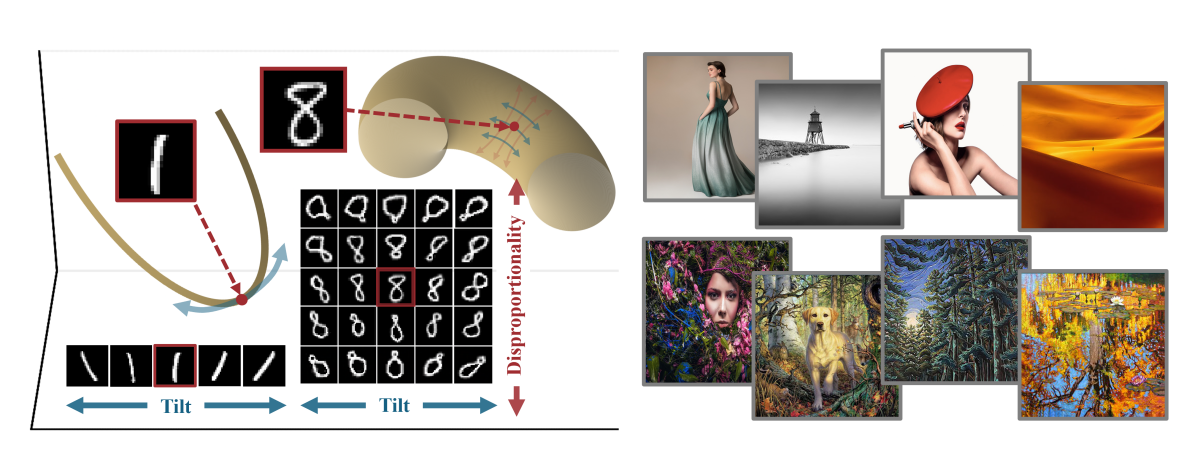
Figure 1: (Left) A cartoon illustration showing that LID is a natural measure of relative complexity. We depict two manifolds of MNIST digits, corresponding to 1s and 8s, as 1-dimensional and 2-dimensional submanifolds of $\mathbb{R}^{3}$, respectively. The relatively simpler manifold of 1s exhibits a single factor of variation (“tilt”), whereas 8s have an additional factor of variation (“disproportionality”). (Right) The 4 lowest- and highest-LID datapoints from a subsample of LAION Aesthetics, as measured by our method, FLIPD, applied to Stable Diffusion v1.5. FLIPD scales efficiently to large models on high-dimensional data, and aligns closely with subjective complexity.

Traditional estimators of intrinsic dimension [21, 37, 42, 11, 29, 19, 1, 5] typically rely on pairwise distances and nearest neighbours, so computing them is prohibitively expensive for large datasets. Recent work has thus sought to move away from these model-free estimators and instead take advantage of deep generative models which learn the distribution of observed data. When this distribution is supported on low-dimensional submanifolds of $\mathbb{R}^{D}$, successful generative models must implicitly learn the dimensions of the data submanifolds, suggesting they can be used to construct LID estimators. However, existing model-based estimators suffer from various drawbacks, including being inaccurate and computationally expensive [57], not leveraging the best existing generative models [60, 68] (i.e. diffusion models [54, 24, 56]), and requiring training several models [60] or altering the training procedure rather than relying on a pre-trained model [25]. Importantly, none of these methods scale to high-resolution images such as those generated by Stable Diffusion [49].

We address all these issues by showing how LID can be efficiently estimated using only a single pre-trained diffusion model (DM) by building on LIDL [60], a model-based estimator. LIDL operates by convolving data with different levels of Gaussian noise, training a normalizing flow [48, 16, 17] for each level, and fitting a linear regression using the log standard deviation of the noise as a covariate and the corresponding log density (of the convolution) evaluated at $x$ as the response; the resulting slope is an estimate of $\text{LID}(x)-D$, thanks to a surprising result linking Gaussian convolutions and LID. We first show how to adapt LIDL to DMs in such a way that only a single DM is required (rather than many normalizing flows). Directly applying this insight leads to LIDL estimates that require one DM but several calls to an ordinary differential equation (ODE) solver; we also show how to circumvent this with an alternative ODE that computes all the required log densities in a single solve. We then argue that the slope of the regression in LIDL aims to capture a rate of change which, for DMs, can be evaluated directly thanks to the Fokker-Planck equation. The resulting estimator, which we call FLIPD, is highly efficient and circumvents the need for an ODE solver.

Our contributions are: $(i)$ showing how DMs can be efficiently combined with LIDL in a way which requires a single call to an ODE solver; $(ii)$ leveraging the Fokker-Planck equation to propose FLIPD, thus improving upon the estimator and circumventing the need for an ODE solver altogether; $(iii)$ motivating FLIPD theoretically; $(iv)$ introducing a suite of LID estimation benchmark tasks highlighting that the previously reported good performance of other estimators is due in part to the simplicity of the tasks over which they were evaluated; $(v)$ demonstrating that FLIPD tends to outperform existing baselines, particularly in high-dimensional settings, while being much more computationally efficient – FLIPD is the first LID estimator to scale to high-resolution images ($\sim 10^{6}$ dimensions), and can be used with Stable Diffusion; and $(vi)$ showing that when applied to natural images, compared to competing alternatives, FLIPD is more aligned both with other measures of complexity such as PNG compression length, and with qualitative assessments of complexity.

2 Background and Related Work

2.1 Diffusion Models

Forward and backward processes

Diffusion models admit various formulations [54, 24]; here we follow the score-based one [56]. We denote the true data-generating distribution, which DMs aim to learn, as $p(\cdot,0)$. DMs define the forward (Itô) stochastic differential equation (SDE),

$${\textnormal{d}}X_{t}=f(X_{t},t){\textnormal{d}}t+g(t){\textnormal{d}}W_{t},\quad X_{0}\sim p(\cdot,0),$$ (1)

where $f:\mathbb{R}^{D}\times[0,1]\rightarrow\mathbb{R}^{D}$ and $g:[0,1]\rightarrow\mathbb{R}$ are hyperparameters, and $W_{t}$ denotes a $D$-dimensional Brownian motion. We write the distribution of $X_{t}$ as $p(\cdot,t)$. The SDE in Equation 1 prescribes how to gradually add noise to data, the idea being that $p(\cdot,1)$ is essentially pure noise. Defining the backward process as $Y_{t}\coloneqq X_{1-t}$, this process obeys the backward SDE [3, 23],

$${\textnormal{d}}Y_{t}=\left[g^{2}(1-t)s(Y_{t},1-t)-f(Y_{t},1-t)\right]{\textnormal{d}}t+g(1-t){\textnormal{d}}\hat{W}_{t},\quad Y_{0}\sim p(\cdot,1),$$ (2)

where $s(x,t)\coloneqq\nabla\log p(x,t)$ is the unknown (Stein) score function, and $\hat{W}_{t}$ is another $D$-dimensional Brownian motion. DMs leverage this backward SDE for generative modelling by using a neural network $\hat{s}:\mathbb{R}^{D}\times(0,1]\rightarrow\mathbb{R}^{D}$ to learn the score function with denoising score matching [64]. Once trained, $\hat{s}(x,t)\approx s(x,t)$. To generate samples $\hat{Y}_{1}$ from the model, we solve an approximation of Equation 2:

$${\textnormal{d}}\hat{Y}_{t}=\left[g^{2}(1-t)\hat{s}(\hat{Y}_{t},1-t)-f(\hat{Y}_{t},1-t)\right]{\textnormal{d}}t+g(1-t){\textnormal{d}}\hat{W}_{t},\quad\hat{Y}_{0}\sim\hat{p}(\cdot,1),$$ (3)

with $\hat{s}$ replacing the true score and with $\hat{p}(\cdot,1)$, a Gaussian distribution chosen to approximate $p(\cdot,1)$ (depending on $f$ and $g$), replacing $p(\cdot,1)$.

Density Evaluation

DMs can be interpreted as continuous normalizing flows [12], and thus admit density evaluation, meaning that if we denote the distribution of $\hat{Y}_{1-t}$ as $\hat{p}(\cdot,t)$, then $\hat{p}(x,t_{0})$ can be mathematically evaluated for any given $x\in\mathbb{R}^{D}$ and $t_{0}\in(0,1]$. More specifically, this is achieved thanks to the (forward) ordinary differential equation (ODE) associated with the DM:

$${\textnormal{d}}\hat{x}_{t}=\left(f(\hat{x}_{t},t)-\dfrac{1}{2}g^{2}(t)\hat{s}(\hat{x}_{t},t)\right){\textnormal{d}}t,\quad\hat{x}_{t_{0}}=x.$$ (4)

Solving this ODE from time $t_{0}$ to time $1$ produces the trajectory $(\hat{x}_{t})_{t\in[t_{0},1]}$, which can then be used for density evaluation through the continuous change-of-variables formula:

$$\log\hat{p}(x,t_{0})=\log\hat{p}(\hat{x}_{1},1)+\int_{t_{0}}^{1}\operatorname{tr}(\nabla v(\hat{x}_{t},t)){\textnormal{d}}t,$$ (5)

where $\hat{p}(\cdot,1)$ can be evaluated since it is a known Gaussian, and where $v(x,t)\coloneqq f(x,t)-g^{2}(t)\hat{s}(x,t)/2$.

Trace estimation

Note that the cost of computing $\nabla v(\hat{x}_{t},t)$ for a particular $\hat{x}_{t}$ amounts to $\mathcal{O}(D)$ function evaluations of $\hat{s}$ (since $D$ calls to a Jacobian-vector-product routine are needed [6]). Although this is not prohibitively expensive for a single $\hat{x}_{t}$, in order to compute the integral in Equation 5 in practice, $(\hat{x}_{t})_{t\in[t_{0},1]}$ must be discretized into a trajectory of length $N$. Deterministic density evaluation is thus computationally intractable as it costs $\mathcal{O}(ND)$ function evaluations. The Hutchinson trace estimator [28] – which states that for $M\in\mathbb{R}^{D\times D}$, $\operatorname{tr}(M)=\mathbb{E}_{\varepsilon}[\varepsilon^{\top}M\varepsilon]$, where $\varepsilon\in\mathbb{R}^{D}$ has mean $0$ and covariance $I_{D}$ – is thus commonly used for stochastic density estimation; approximating the expectation with $k$ samples from $\varepsilon$ results in a cost of $\mathcal{O}(Nk)$, which is much faster than deterministic density evaluation when $k\ll D$.

2.2 Local Intrinsic Dimension and How to Estimate It

LID

Various definitions of intrinsic dimension exist [27, 20, 36], here we follow the standard one from geometry: a $d$-dimensional manifold is a set which is locally homeomorphic to $\mathbb{R}^{d}$. For a given disjoint union of manifolds and a point $x$ in this union, the local intrinsic dimension of $x$ is the dimension of the manifold it belongs to. Note that LID is not an intrinsic property of the point $x$, but rather a property of $x$ with respect to the manifold that contains it. Intuitively, $\text{LID}(x)$ corresponds to the number of factors of variation present in the manifold containing $x$, and it is thus a natural measure of the relative complexity of $x$, as illustrated in Figure 1.

Estimating LID

The natural interpretation of LID as a measure of complexity makes estimating it from observed data a relevant problem. Here, the formal setup is that $p(\cdot,0)$ is supported on a disjoint union of manifolds [10], and we assume access to a dataset sampled from it. Then, for a given $x$ in the support of $p(\cdot,0)$, we want to use the dataset to provide an estimate of $\text{LID}(x)$. Traditional estimators [21, 37, 42, 11, 29, 19, 1, 5] rely on the nearest neighbours of $x$ in the dataset, or related quantities, and typically have poor scaling in dataset size. Generative models are an intuitive alternative to these methods; because they are trained to learn $p(\cdot,0)$, when they succeed they must encode information about the support of $p(\cdot,0)$, including the corresponding manifold dimensions. However, extracting this information from a trained generative model is not trivial. For example, Zheng et al. [68] showed that the number of active dimensions in the approximate posterior of variational autoencoders [32, 48] estimates LID, but their approach does not generalize to better generative models.

LIDL

Tempczyk et al. [60] proposed LIDL, a method for LID estimation relying on normalizing flows as tractable density estimators [48, 16, 17]. LIDL works thanks to a surprising result linking Gaussian convolutions and LID [38, 60, 68]. We will denote the convolution of $p(\cdot,0)$ and Gaussian noise with log standard deviation $\delta$ as $\varrho(\cdot,\delta)$, i.e.

$$\varrho(x,\delta)\coloneqq\int p(x_{0},0)\mathcal{N}(x-x_{0};0,e^{2\delta}I_{D}){\textnormal{d}}x_{0}.$$ (6)

The aforementioned result states that, under mild regularity conditions on $p(\cdot,0)$, and for a given $x$ in its support, the following holds as $\delta\rightarrow-\infty$:

$$\log\varrho(x,\delta)=\delta(\text{LID}(x)-D)+\mathcal{O}(1).$$ (7)

This result then suggests that, for negative enough values of $\delta$ (i.e. small enough standard deviations):

$$\log\varrho(x,\delta)\approx\delta(\text{LID}(x)-D)+c,$$ (8)

for some constant $c$. If we could evaluate $\log\varrho(x,\delta)$ for various values of $\delta$, this would provide an avenue for estimating $\text{LID}(x)$: set some values $\delta_{1},\dots,\delta_{m}$, fit a linear regression using $\{(\delta_{i},\log\varrho(x,\delta_{i}))\}_{i=1}^{m}$ (with $\delta$ as the covariate and $\log\varrho(x,\delta)$ as the response), and let $\hat{\beta}_{x}$ be the corresponding slope. It follows that $\hat{\beta}_{x}$ estimates $\text{LID}(x)-D$, so that $\text{LID}(x)\approx D+\hat{\beta}_{x}$ is a sensible estimator of local intrinsic dimension.

Since $\varrho(x,\delta)$ is unknown and cannot be evaluated, LIDL requires training $m$ normalizing flows. More specifically, for each $\delta_{i}$, a normalizing flow is trained on data to which $\mathcal{N}(0,e^{2\delta_{i}}I_{D})$ noise is added. In LIDL, the log densities of the trained models are then used instead of the unknown true log densities $\log\varrho(x,\delta_{i})$ when fitting the regression as described above.

Despite using generative models, LIDL has obvious drawbacks. LIDL requires training several models. It also relies on normalizing flows, which are not only empirically outperformed by DMs by a wide margin, but are also known to struggle to learn low-dimensional manifolds [13, 38, 39]. On the other hand, DMs do not struggle to learn $p(\cdot,0)$ even when it is supported on low-dimensional manifolds [46, 15, 39], further suggesting that LIDL can be improved by leveraging DMs.

Estimating LID with DMs

The only works we are aware of that leverage DMs for LID estimation are those of Stanczuk et al. [57], and Horvat and Pfister [25]. The latter modifies the training procedure of DMs, so we focus on the former since we see compatibility with existing pre-trained models as an important requirement for DM-based LID estimators. Stanczuk et al. consider variance-exploding DMs, where $f=0$. They show that, as $t\searrow 0$, the score function $s(x,t)$ points orthogonally towards the manifold containing $x$, or more formally, it lies in the normal space of this manifold at $x$. They thus propose the following LID estimator which we refer to as the normal bundle (NB) estimator: first run Equation 1 until time $t_{0}$ starting from $x$, and evaluate $\hat{s}(\cdot,t_{0})$ at the resulting value; then repeat this process $K$ times and stack the $K$ resulting $D$-dimensional vectors into a matrix $S(x)\in\mathbb{R}^{D\times K}$. The idea here is that if $t_{0}$ is small enough and $K$ is large enough, the columns of $S(x)$ span the normal space of the manifold at $x$, suggesting that the rank of this matrix estimates the dimension of this normal space, namely $D-\text{LID}(x)$. Finally, they estimate $\text{LID}(x)$ as:

$$\text{LID}(x)\approx D-\operatorname{rank}S(x).$$ (9)

Although this estimator addresses some of the limitations of LIDL, it remains computationally expensive – computing $S(x)$ requires $K$ function evaluations with the authors recommending $K=4D$ – and as we will see later, it does not always produce reliable estimates.

3 Method

Although Tempczyk et al. [60] only used normalizing flows in LIDL, they did point out that these models could be swapped for any other generative model admitting density evaluation. Indeed, one could trivially train $m$ DMs and replace the flows with them. Throughout this section we will assume access to a pre-trained DM such that $f(x,t)=b(t)x$ for a function $b:[0,1]\rightarrow\mathbb{R}$. This choice implies that the transition kernel $p_{t|0}$ associated with Equation 1 is Gaussian [51]:

$$p_{t\mid 0}(x_{t}\mid x_{0})=\mathcal{N}(x_{t};\psi(t)x_{0},\sigma^{2}(t)I_{D}),$$ (10)

where $\psi,\sigma:[0,1]\rightarrow\mathbb{R}$. We also assume that $b$ and $g$ are such that $\psi$ and $\sigma$ are differentiable and such that $\lambda(t)\coloneqq\sigma(t)/\psi(t)$ is injective. This setting encompasses all DMs commonly used in practice, including variance-exploding, variance-preserving (of which DDPM [24] is a discretized instance), and sub-variance-preserving [56]. In Appendix A we include explicit formulas for $\psi(t)$, $\sigma^{2}(t)$, and $\lambda(t)$ for these particular DMs.

3.1 LIDL with a Single Diffusion Model

As opposed to the several normalizing flows used in LIDL which are individually trained on datasets with different levels of noise added, a single DM already works by convolving data with various noise levels and allows density evaluation of the resulting noisy distributions (Equation 5). Hence, we make the observation that LIDL can be used with a single DM. All we need is to relate $\varrho(x,\delta)$ to the density of the DM for any given $x$ and $\delta$. In the case of variance-exploding DMs, $\psi(t)=1$, so we can easily use the defining property of the transition kernel in Equation 10 to get

$$p(x,t)=\int p(x_{0},0)p_{t\mid 0}(x_{t}\mid x_{0}){\textnormal{d}}x_{0}=\int p(x_{0},0)\mathcal{N}(x_{t};x_{0},\sigma^{2}(t)I_{D}){\textnormal{d}}x_{0},$$ (11)

which equals $\varrho(x,\delta)$ from Equation 6 when we choose $t=\sigma^{-1}(e^{\delta})$. In turn, we can use LIDL with a single variance-exploding DM by evaluating each $\hat{p}(x,\sigma^{-1}(e^{\delta_{i}}))$ through Equation 5. This idea extends beyond variance-exploding DMs; in Appendix B.1 we show that for any arbitrary DM with transition kernel as in Equation 10, it holds that

$$\log\varrho(x,\delta)=D\log\psi\big{(}t(\delta)\big{)}+\log p\Big{(}\psi\big{(}t(\delta)\big{)}x,t(\delta)\Big{)},$$ (12)

where $t(\delta)\coloneqq\lambda^{-1}(e^{\delta})$, thus showing that LIDL can be used with a single DM.

3.2 An Efficient Implementation of LIDL with Diffusion Models

Using Equation 12 with LIDL still involves computing $\log\hat{p}\big{(}\psi(t(\delta_{i}))x,t(\delta_{i})\big{)}$ through Equation 5 for each $i=1,\dots,m$ before running the regression. Since each of the corresponding ODEs in Equation 4 starts at a different time $t_{0}=t(\delta_{i})$ and is evaluated at a different point $\psi(t(\delta_{i}))x$, this means that a different ODE solver call would have to be used for each $i$, resulting in a prohibitively expensive procedure. By leveraging the Fokker-Planck equation associated with Equation 1, we show in Appendix B.2 that, for DMs with transition kernel as in Equation 10,

(13)

Assuming without loss of generality that $\delta_{1}<\dots<\delta_{m}$, solving the ODE

$${\textnormal{d}}\log\hat{\varrho}(x,\delta)=\nu\big{(}t(\delta);\hat{s},x\big{)}{\textnormal{d}}\delta,\quad\log\hat{\varrho}(x,\delta_{1})=0,$$ (14)

from $\delta_{1}$ to $\delta_{m}$ produces the trajectory $(\log\hat{\varrho}(x,\delta))_{\delta\in[\delta_{1},\delta_{m}]}$. Since $\nu(t(\delta);\hat{s},x)$ does not depend on $\hat{\varrho}(x,\delta)$, when $\hat{s}=s$ the solution will be such that $\log\hat{\varrho}(x,\delta)=\log\varrho(x,\delta)+c_{\text{init}}$ for some constant $c_{\text{init}}$ that depends on the initial condition but not on $\delta$. Thus, while setting the initial condition to $0$ might at first appear odd, we can fit a regression as in LIDL, using $\{(\delta_{i},\log\hat{\varrho}(x,\delta_{i}))\}_{i=1}^{m}$, and $c_{\text{init}}$ will be absorbed in the intercept without affecting the slope. In other words, the initial condition is irrelevant, and we can use LIDL with DMs by calling a single ODE solver on Equation 14.

3.3 FLIPD: A Fokker-Planck-Based LID Estimator

The LIDL estimator with DMs presented in subsection 3.2 provides a massive speedup over the naïve approach of training $m$ DMs, and over the method from subsection 3.1 requiring $m$ ODE solves. Yet, solving Equation 14 involves computing the trace of the Jacobian of $\hat{s}$ multiple times within an ODE solver, which, as mentioned in subsection 2.1, remains expensive. In this section we present our LID estimator, FLIPD, which circumvents the need for an ODE solver altogether. Recall that LIDL is based on Equation 8, which justifies the regression. Differentiating this equation yields that $\partial\log\varrho(x,\delta_{0})/\partial\delta\approx\text{LID}(x)-D$ for negative enough $\delta_{0}$, meaning that Equation 13 directly provides the rate of change that the regression in LIDL aims to estimate, from which we get

$$\text{LID}(x)\approx D+\dfrac{\partial}{\partial\delta}\log\varrho(x,\delta_{0})\approx D+\nu\big{(}t(\delta_{0});\hat{s},x\big{)}\eqqcolon\text{FLIPD}(x,t_{0}),$$ (15)

where $t_{0}\coloneqq t(\delta_{0})$. In addition to not requiring an ODE solver, computing FLIPD requires setting only a single hyperparameter, whereas regression-based estimators require $m$. Since $\nu(t(\delta);\hat{s},x)$ depends on $\delta$ only through $t(\delta)$, we can directly set $t_{0}$ as the hyperparameter rather than $\delta_{0}$, which avoids the potentially cumbersome computation of $t(\delta_{0})=\lambda^{-1}(e^{\delta_{0}})$: instead of setting a suitably negative $\delta_{0}$, we set $t_{0}>0$ sufficiently close to $0$. In Appendix A we include explicit formulas for $\text{FLIPD}(x,t_{0})$ for common DMs.

Finally, we present a theoretical result further justifying FLIPD. Note that the $\mathcal{O}(1)$ term in Equation 7 need not be constant in $\delta$ as in Equation 8, even if it is bounded. The more this term deviates from a constant, the more bias we should expect in both LIDL and FLIPD. The following result shows that in an idealized linear setting, FLIPD is unaffected by this problem:

Theorem 3.1.

Let $\mathcal{L}$ be an embedded submanifold of $\mathbb{R}^{D}$ given by a $d$-dimensional affine subspace. If $p(\cdot,0)$ is supported on $\mathcal{L}$, continuous, and with finite second moments, then for any $x\in\mathcal{L}$ with $p(x,0)>0$, we have:

$$\lim_{\delta\rightarrow-\infty}\dfrac{\partial}{\partial\delta}\log\varrho(x,\delta)=d-D.$$ (16)

Proof.

See Appendix B.3. ∎

We hypothesize that this result can be extended to non-linear submanifolds since, intuitively, every manifold can be locally linearly approximated (by its tangent space) and $\varrho(x,\delta)$ is “local as $\delta\rightarrow-\infty$” in the sense that its dependence on the values $p(y,0)$ becomes negligible as $\delta\rightarrow-\infty$ (because $\mathcal{N}(0,e^{2\delta}I_{D})$ approaches a point mass at $0$) when $y$ is not in a close enough neighbourhood of $x$. However, we leave generalizing our result to future work.

4 Experiments

Throughout our experiments, we use variance-preserving DMs, the most popular variant of DMs, and compatible with DDPMs. We also include a “dictionary” to translate between the score-based formulation under which we developed FLIPD, and DDPMs, in Appendix C. Our code is available at https://github.com/layer6ai-labs/flipd; see Appendix D.1 for our hyperparameter setup.

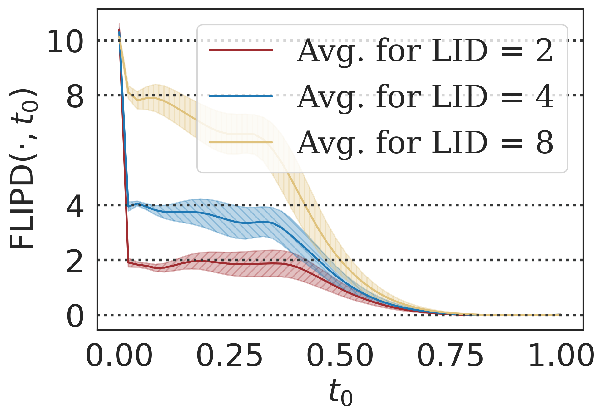
(a) Mixture of Gaussians.

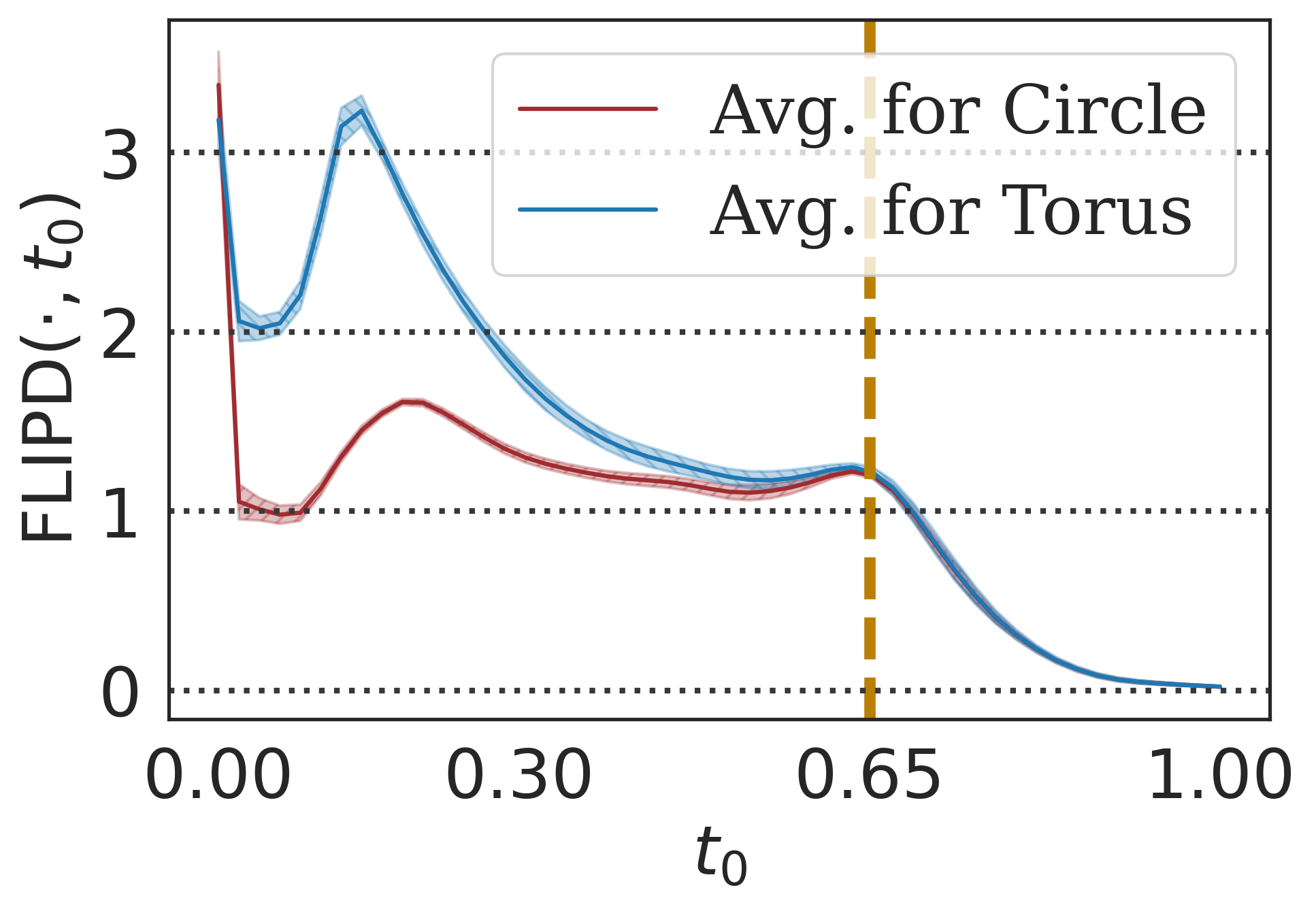
(b) String within a doughnut.

Figure 2: FLIPD curves with knees at the true LID.

The effect of $t_{0}$

FLIPD requires setting $t_{0}$ close to $0$ (since all the theory holds in the $\delta\rightarrow-\infty$ regime). It is important to note that DMs fitted to low-dimensional manifolds are known to exhibit numerically unstable scores $s(\cdot,t_{0})$ as $t_{0}\searrow 0$ [62, 40, 39]. Our first set of experiments examines the effect of $t_{0}$ on $\text{FLIPD}(x,t_{0})$ by varying $t_{0}$ within the range $(0,1)$.

In Figure 2, we train DMs on two distributions: $(i)$ a mixture of three isotropic Gaussians with dimensions $2$, $4$, and $8$, embedded in $\mathbb{R}^{10}$ (each embedding is carried out by multiplication against a random matrix with orthonormal columns plus a random translation); and $(ii)$ a “string within a doughnut”, which is a mixture of uniform distributions on a 2d torus (with a major radius of $10$ and a minor radius of $1$) and a 1d circle (aligning with the major circle of the torus) embedded in $\mathbb{R}^{3}$ (this union of manifolds is shown in the upper half of Figure 3). While $\text{FLIPD}(x,t_{0})$ is inaccurate at $t_{0}=0$ due to the aforementioned instabilities, it quickly stabilizes around the true LID for all datapoints. We refer to this pattern as a knee in the FLIPD curve. In Appendix D.2, we show similar curves for more complex data manifolds.

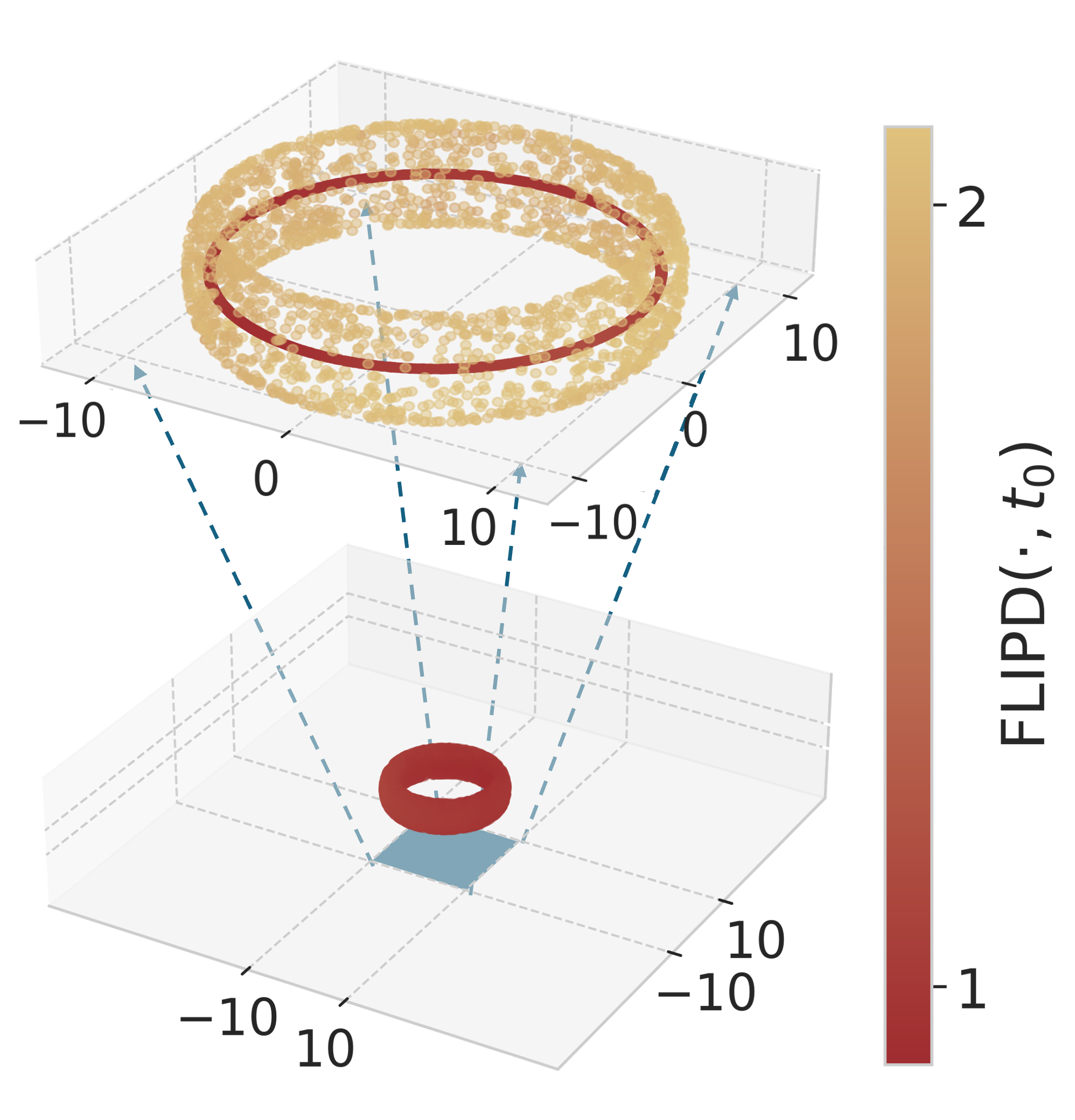
Figure 3: “String within a doughnut” manifolds, and corresponding FLIPD estimates for different values of $t_{0}$ ($t_{0}=0.05$ on top and $t_{0}=0.65$ on bottom). These results highlight the multiscale nature of FLIPD.

FLIPD is a multiscale estimator

Interestingly, in 2(b) we see that the blue FLIPD curve (corresponding to “doughnut” points with LID of $2$) exhibits a second knee at $1$, located at the $t_{0}$ shown with a vertical line. This confirms the multiscale nature of convolution-based estimators, first postulated by Tempczyk et al. [60] in the context of normalizing flows; they claim that when selecting a log standard deviation $\delta$, all directions along which a datum can vary having log standard deviation less than $\delta$ are ignored. The second knee in 2(b) can be explained by a similar argument: the torus looks like a 1d circle when viewed from far away, and larger values of $t_{0}$ correspond to viewing the manifolds from farther away. This is visualized in Figure 3 with two views of the “string within a doughnut” and corresponding LID estimates: one zoomed-in view where $t_{0}$ is small, providing fine-grained LID estimates, and a zoomed-out view where $t_{0}$ is large, making both the string and doughnut appear as a 1d circle from this distance. In Appendix D.3 we have an experiment that makes the multiscale argument explicit.

Finding knees

As mentioned, we persistently see knees in FLIPD curves. This in line with the observations of Tempczyk et al. [60] (see Figure 5 of [60]), and it gives us a fully automated approach to setting $t_{0}$. We leverage kneedle [52], a knee detection algorithm which aims to find points of maximum curvature. When computationally sensible, rather than fixing $t_{0}$, we evaluate Equation 15 for $50$ values of $t_{0}$ and pass the results to kneedle to automatically detect the $t_{0}$ where a knee occurs.

Table 1: MAE (lower is better) $\mid$ concordance indices (higher is better with $1.0$ being the gold standard). Rows show synthetic manifolds and columns represent LID estimation methods. Columns are grouped based on whether they use a generative model, with the best results for each metric within each group being bolded.

	Model-based						Model-free
Synthetic Manifold	FLIPD		NB		LIDL		ESS		LPCA
String within doughnut $\subseteq\mathbb{R}^{3}$	$\mathbf{0.06}$	$\mathbf{{\color[rgb]{0.64705882,0.43921569,0.2}1.00}}$	$1.48$	${\color[rgb]{0.64705882,0.43921569,0.2}0.48}$	$1.10$	${\color[rgb]{0.64705882,0.43921569,0.2}0.99}$	$0.02$	$\mathbf{{\color[rgb]{0.64705882,0.43921569,0.2}1.00}}$	$\mathbf{0.00}$	$\mathbf{{\color[rgb]{0.64705882,0.43921569,0.2}1.00}}$
$\mathcal{L}_{5}\subseteq\mathbb{R}^{10}$	$0.17$	-	$1.00$	-	$\mathbf{0.10}$	-	$0.07$	-	$\mathbf{0.00}$	-
$\mathcal{N}_{90}\subseteq\mathbb{R}^{100}$	$0.49$	-	$\mathbf{0.18}$	-	$0.33$	-	$\mathbf{1.67}$	-	$21.9$	-
$\mathcal{U}_{10}+\mathcal{U}_{30}+\mathcal{U}_{90}\subseteq\mathbb{R}^{100}$	$\mathbf{1.30}$	$\mathbf{{\color[rgb]{0.64705882,0.43921569,0.2}1.00}}$	$61.6$	${\color[rgb]{0.64705882,0.43921569,0.2}0.34}$	$8.46$	${\color[rgb]{0.64705882,0.43921569,0.2}0.74}$	$21.9$	${\color[rgb]{0.64705882,0.43921569,0.2}0.74}$	$\mathbf{20.1}$	$\mathbf{{\color[rgb]{0.64705882,0.43921569,0.2}0.86}}$
$\mathcal{N}_{10}+\mathcal{N}_{25}+\mathcal{N}_{50}\subseteq\mathbb{R}^{100}$	$\mathbf{1.81}$	$\mathbf{{\color[rgb]{0.64705882,0.43921569,0.2}1.00}}$	$74.2$	${\color[rgb]{0.64705882,0.43921569,0.2}0.34}$	$8.87$	${\color[rgb]{0.64705882,0.43921569,0.2}0.74}$	$7.71$	${\color[rgb]{0.64705882,0.43921569,0.2}0.88}$	$\mathbf{5.72}$	$\mathbf{{\color[rgb]{0.64705882,0.43921569,0.2}0.91}}$
$\mathcal{F}_{10}+\mathcal{F}_{25}+\mathcal{F}_{50}\subseteq\mathbb{R}^{100}$	$\mathbf{3.93}$	$\mathbf{{\color[rgb]{0.64705882,0.43921569,0.2}1.00}}$	$74.2$	${\color[rgb]{0.64705882,0.43921569,0.2}0.34}$	$18.6$	${\color[rgb]{0.64705882,0.43921569,0.2}0.70}$	$9.20$	${\color[rgb]{0.64705882,0.43921569,0.2}0.90}$	$\mathbf{6.77}$	$\mathbf{{\color[rgb]{0.64705882,0.43921569,0.2}1.00}}$
$\mathcal{U}_{10}+\mathcal{U}_{80}+\mathcal{U}_{200}\subseteq\mathbb{R}^{800}$	$\mathbf{14.3}$	$\mathbf{{\color[rgb]{0.64705882,0.43921569,0.2}1.00}}$	$715$	${\color[rgb]{0.64705882,0.43921569,0.2}0.34}$	$120$	${\color[rgb]{0.64705882,0.43921569,0.2}0.70}$	$1.39$	$\mathbf{{\color[rgb]{0.64705882,0.43921569,0.2}1.00}}$	$\mathbf{0.01}$	$\mathbf{{\color[rgb]{0.64705882,0.43921569,0.2}1.00}}$
$\mathcal{U}_{900}\subseteq\mathbb{R}^{1000}$	$\mathbf{12.8}$	-	$100$	-	$24.9$	-	$\mathbf{14.5}$	-	$219$	-

Synthetic experiments

We create a benchmark for LID evaluation on complex unions of manifolds where the true LID is known. We sample from simple distributions on low-dimensional spaces, and then embed the samples into $\mathbb{R}^{D}$. We denote uniform, Gaussian, and Laplace distributions as $\mathcal{U},\mathcal{N}$, and $\mathcal{L}$, respectively, with sub-indices indicating LID, and a plus sign denoting mixtures. To embed samples into higher dimensions, we apply a random matrix with orthonormal columns and then apply a random translation. For example, $\mathcal{N}_{10}+\mathcal{L}_{20}\subseteq\mathbb{R}^{100}$ indicates a $10$-dimensional Gaussian and a $20$-dimensional Laplace, each of which undergoes a random affine transformation mapping to $\mathbb{R}^{100}$ (one transformation per component). We also generate non-linear manifolds, denoted with $\mathcal{F}$, by applying a randomly initialized $D$-dimensional neural spline flow [17] after the affine transformation (when using flows, the input noise is always uniform); since the flow is a diffeomorphism, it preserves LID. To our knowledge, this synthetic LID benchmark is the most extensive to date, revealing surprising deficiencies in some well-known traditional estimators. For an in-depth analysis, see Appendix D.4.

Here, we summarize our synthetic experiments in Table 1 using two metrics of performance: the mean absolute error (MAE) between the predicted and true LID for individual datapoints; and the concordance index, which measures similarity in the rankings between the true LIDs and the estimated ones (note that this metric only makes sense when the dataset has variability in its ground truth LIDs, so we only report it for the appropriate entries in Table 1). We compare against the NB and LIDL estimators described in subsection 2.2, as well as two of the most performant model-free baselines: LPCA [21, 11] and ESS [29]. For the NB baseline, we use the exact same DM backbone as for FLIPD (since NB was designed for variance-exploding DMs, we use the adaptation to variance-preserving DMs used in [31], which produces extremely similar results), and for LIDL we use $8$ neural spline flows. In terms of MAE, we find that FLIPD tends to be the best model-based estimator, particularly as dimension increases. Although model-free baselines perform well in simplistic scenarios, they produce unreliable results as LID increases or more non-linearity is introduced in the data manifold. In terms of concordance index, FLIPD achieves perfect scores in all scenarios, meaning that even when its estimates are off, it always provides correct LID rankings. We include additional results in the appendices: in Appendix D.5 we ablate FLIPD, finding that using kneedle indeed helps, and that FLIPD also outperforms the efficient implementation of LIDL with DMs described in subsection 3.2 that uses an ODE solver. We notice that NB with the setting proposed in [57] consistently produces estimates that are almost equal to the ambient dimension; thus, in Appendix D.6 we also show how NB can be significantly improved upon by using kneedle, although it is still outperformed by FLIPD in many scenarios. In addition, in Tables 6 and 7 we compare against other model-free baselines such as MLE [37, 42] and FIS [1]. We also consider datasets with a single (uni-dimensional) manifold where the average LID estimate can be used to approximate the global intrinsic dimensionality. Our results in Table 8 demonstrate that although model-free baselines indeed accurately estimate the global intrinsic dimension, they perform poorly when focusing on their pointwise LID estimates.

Image experiments

We first focus on the simple image datasets MNIST [35] and FMNIST [66]. We flatten the images and use the same MLP architecture as in our synthetic experiments. Despite using an MLP, our DMs can generate reasonable samples (Appendix E.1) and the FLIPD curve for both MNIST and FMNIST is shown in 4(a). The knee points are identified at $t_{0}=0.1$, resulting in average LID estimates of approximately $130$ and $170$, respectively. Evaluating LID estimates for image data is challenging due to the lack of ground truth. Although our LID estimates are higher than those in [47] and [10], our experiments (Table 8 of Appendix D.4) and findings in [60] and [57] show that model-free baselines underestimate LID of high-dimensional data, especially images.

When moving to more complex image datasets, the simplistic MLP score network backbone fails to generate high-quality samples. Therefore, we replace it with state-of-the-art UNets [50, 65] (see Appendix E.2). As long as the DM accurately fits the data manifold, our theory should hold, regardless of the choice of backbone. Yet, we see that UNets do not produce a clear knee in the FLIPD curves (see curves in Figure 10 of Appendix E.1). We discuss why this might be the case in Appendix E.1, and from here on we simply set $t_{0}$ as a hyperparameter instead of using kneedle. Despite FLIPD curves lacking a knee when using UNets, we argue that our estimates remain valuable measures of complexity. We took random subsets of $4096$ images from each of FMNIST, MNIST, SVHN [45], and CIFAR10 [34], and sorted them according to their FLIPD estimates. We show the top and bottom 5 images for each dataset in 4(b), and include more samples in Appendix E.3. Our visualization shows that higher FLIPD estimates indeed correspond to images with more detail and texture, while lower estimates correspond to less complex ones. Additionally, we show in Appendix E.4 that using only $50$ Hutchinson samples to approximate the trace term in FLIPD is sufficient for small values of $t_{0}$: FLIPD not only visually corresponds to image complexity, but also required only $50$ Jacobian-vector-products, resulting in a significant speedup over all prior work.

Table 2: Spearman’s correlation between LID estimates and PNG compression size.

Method	MNIST	FMNIST	CIFAR10	SVHN
FLIPD	$0.837$	$\mathbf{0.883}$	$0.819$	$\mathbf{0.876}$
NB	$\mathbf{0.864}$	$0.480$	$\mathbf{0.894}$	$0.573$
ESS	$0.444$	$0.063$	$0.326$	$0.019$
LPCA	$0.413$	$0.01$	$0.302$	$-0.008$

Further, we quantitatively assess our estimates by computing Spearman’s rank correlation coefficient between different LID estimators and PNG compression size, used as a proxy for complexity in the absence of ground truth. As shown in Table 2, FLIPD has a high correlation with PNG, whereas model-free estimators do not. We find that the NB estimator correlates slightly more with PNG on MNIST and CIFAR10, but significantly less in FMNIST and SVHN. We also highlight that NB requires $\sim 3000$ function evaluations to produce a single LID estimate for MNIST and FMNIST, and $\sim 12000$ for SVHN and CIFAR10 – a massive increase in computation as compared to the $50$ Jacobian-vector-products we used for FLIPD. Moreover, in Appendix E.5, we analyze how increasing $t_{0}$ affects the estimator by re-computing the correlation with the PNG size at different values of $t_{0}\in(0,1)$. We see that as $t_{0}$ increases, the correlation with PNG decreases. Despite this decrease, we observe an interesting phenomenon: while characteristics of the image orderings change, qualitatively, the smallest $\text{FLIPD}(\cdot,t_{0})$ estimates still represent less complex data compared to the highest $\text{FLIPD}(\cdot,t_{0})$, even for relatively large $t_{0}$. We hypothesize that for larger $t_{0}$, similar to the “string within a doughnut” experiment in Figure 3, the orderings correspond to coarse-grained and semantic notions of complexity rather than fine-grained ones such as textures, concepts that a metric such as PNG size cannot capture.

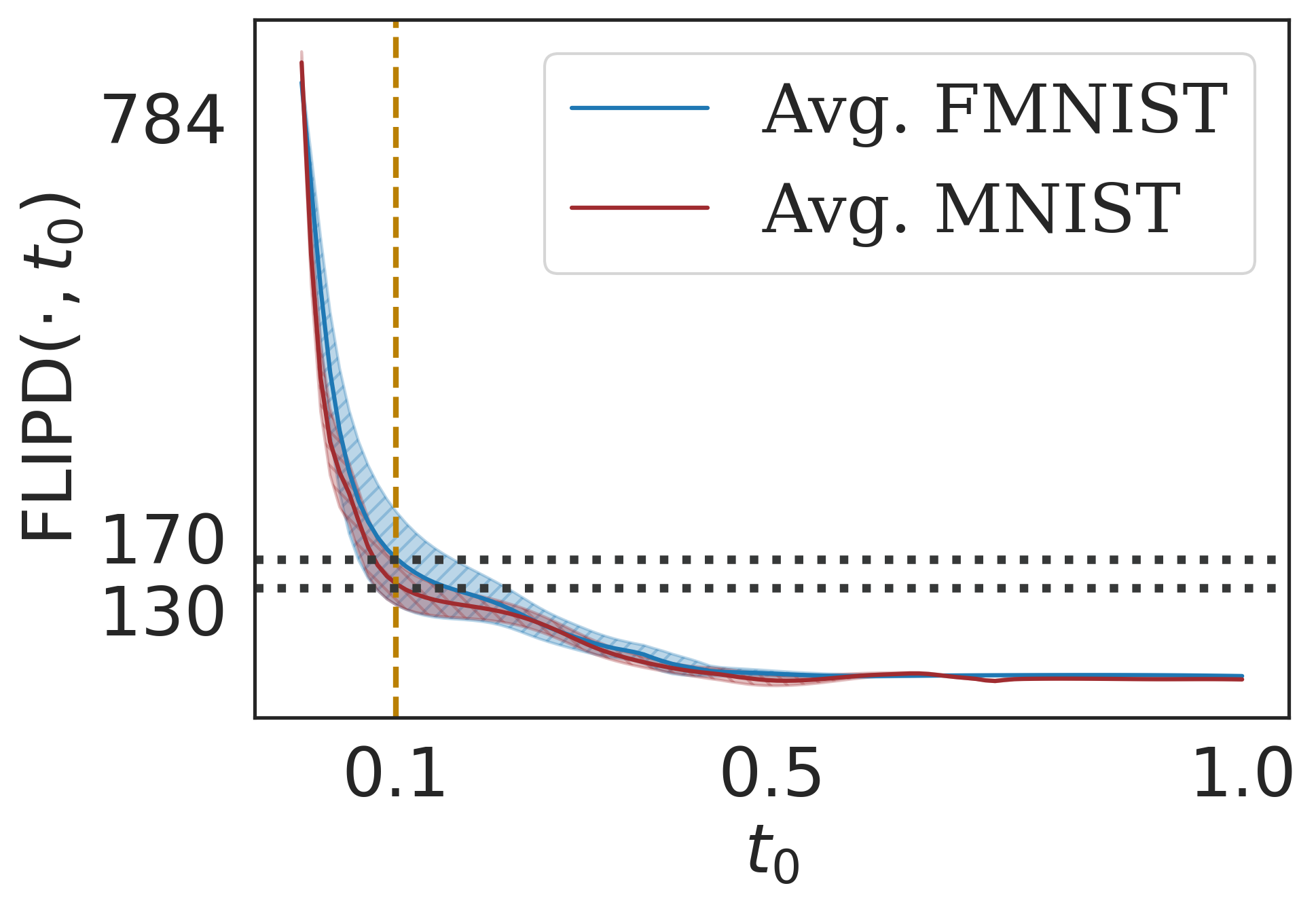
(a) FLIPD of MNIST and FMNIST.

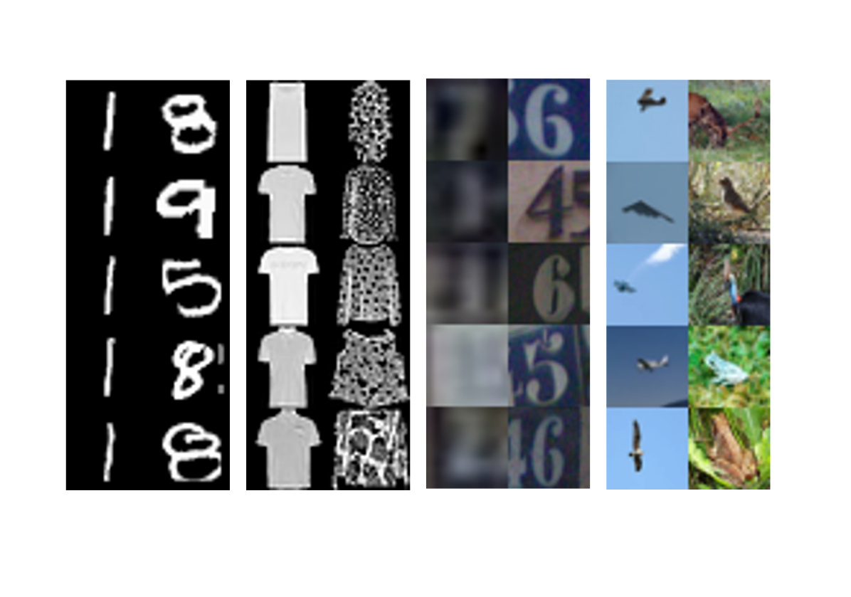
(b) Ordering small images.

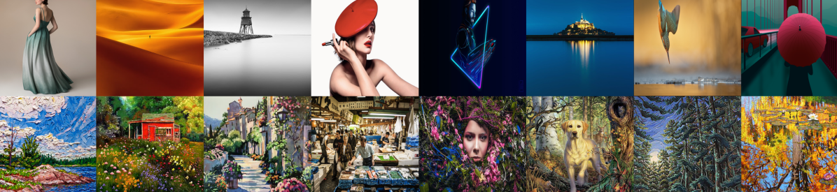
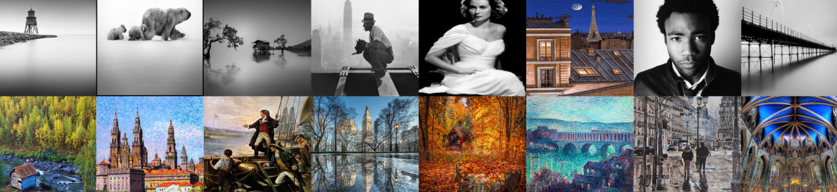
(c) Ordering high-resolution images in LAION using FLIPD (top) and PNG compression size (bottom).

Figure 4: Overview of image LID: (a) shows the FLIPD curves that are used to estimate average LID for MNIST and FMNIST; (b) compares images with small and large FLIPD estimates from FMNIST, MNIST, SVHN, and CIFAR10; and (c) compares LAION images with small and large FLIPD estimates using Stable Diffusion (top, $t_{0}=0.5$) and PNG compression sizes (bottom).

Finally, we consider high-resolution images from LAION-Aesthetics [53] and, for the first time, estimate LID for extremely high-dimensional images with $D=3\times 512\times 512=786,\!432$. We use Stable Diffusion [49], a latent DM pretrained on LAION-5B [53]. This includes an encoder and a decoder trained to preserve relevant characteristics of the data manifold in latent representations. Since the encoder and decoder are continuous and effectively invert each other, we argue that the Stable Diffusion encoder can, for practical purposes, be considered a topological embedding of the LAION-5B dataset into its latent space of dimension $4\times 64\times 64=16,\!384$. Therefore, the dimension of the LAION-5B submanifold in latent space should be unchanged. We thus estimate image LIDs by carrying out FLIPD in the latent space of Stable Diffusion. Here, we set the Hutchinson sample count to $1$, meaning we only require a single Jacobian-vector-product. When we order a random subset of $1600$ samples according to their FLIPD at $t_{0}=0.3$, the more complex images are clustered at the end, while the least complex are clustered at the beginning: see Figure 1 and 4(c) for the lowest- and highest-LID images from this ordering, and Figure 25 in Appendix E.6 to view the entire subset and other values of $t_{0}$. In comparison to orderings according to PNG compression size (4(c)), FLIPD estimates prioritize semantic complexity over low-level details like colouration.

5 Conclusions, Limitations, and Future Work

In this work we have shown that the Fokker-Planck equation can be utilized for efficient LID estimation with any pre-trained DM. We have provided strong theoretical foundations and extensive benchmarks showing that FLIPD estimates accurately reflect data complexity. Although FLIPD produces excellent LID estimates on synthetic benchmarks, the lack of knees in FLIPD curves on image data when using state-of-the-art architectures is surprising, and results in unstable LID estimates which strongly depend on $t_{0}$. We see this behaviour as a limitation, even if FLIPD provides a meaningful measure of complexity in these cases. Given that FLIPD is tractable, differentiable, and compatible with any DM, we hope that it will find uses in applications where LID estimates have already proven helpful, including OOD detection, AI-generated data analysis, and adversarial example detection.

Appendix A Explicit Formulas

A.1 Variance-Exploding Diffusion Models

Variance-exploding DMs are such that $f(x,t)=0$ with $g$ being non-zero. In this case [56]:

$$\psi(t)=1,\quad\text{and}\quad\sigma^{2}(t)=\int_{0}^{t}g^{2}(u){\textnormal{d}}u.$$ (17)

Since $g$ is non-zero, $g^{2}$ is positive, so that $\sigma^{2}$ is increasing, and thus injective. It follows that $\sigma$ is also injective, so that $\lambda=\sigma/\psi=\sigma$ is injective. Equation 15 then implies that

$$\text{FLIPD}(x,t_{0})=D+\sigma^{2}(t_{0})\left[\operatorname{tr}\big{(}\nabla s(x,t_{0})\big{)}+\|s(x,t_{0})\|_{2}^{2}\right].$$ (18)

A.2 Variance-Preserving Diffusion Models (DDPMs)

Variance-preserving DMs are such that

$$f(x,t)=-\dfrac{1}{2}\beta(t)x,\quad\text{and}\quad g(t)=\sqrt{\beta(t)},$$ (19)

where $\beta$ is a positive scalar function. In this case [56]:

$$\psi(t)=e^{-\tfrac{1}{2}B(t)},\quad\text{and}\quad\sigma^{2}(t)=1-e^{-B(t)},\quad\text{where}\quad B(t)\coloneqq\int_{0}^{t}\beta(u){\textnormal{d}}u.$$ (20)

We then have that

$$\lambda(t)=\sqrt{\dfrac{\sigma^{2}(t)}{\psi^{2}(t)}}=\sqrt{e^{B(t)}-1}.$$ (21)

Since $\beta$ is positive, $B$ is increasing and thus injective, from which it follows that $\lambda$ is injective as well. Plugging everything into Equation 15, we obtain:

$$\text{FLIPD}(x,t_{0}) =D+\big{(}1-e^{-B(t_{0})}\big{)}\left(\operatorname{tr}\Big{(}\nabla s\big{(}e^{-\tfrac{1}{2}B(t_{0})}x,t_{0}\big{)}\Big{)}+\big{\|}s\big{(}e^{-\tfrac{1}{2}B(t_{0})}x,t_{0}\big{)}\big{\|}_{2}^{2}\right).$$ (22)

A.3 Sub-Variance-Preserving Diffusion Models

Sub-variance-preserving DMs are such that

$$f(x,t)=-\dfrac{1}{2}\beta(t)x,\quad\text{and}\quad g(t)=\sqrt{\beta(t)\left(1-e^{-2B(t)}\right)},\quad\text{where}\quad B(t)\coloneqq\int_{0}^{t}\beta(u){\textnormal{d}}u,$$ (23)

and where $\beta$ is a positive scalar function. In this case [56]:

$$\psi(t)=e^{-\tfrac{1}{2}B(t)},\quad\text{and}\quad\sigma^{2}(t)=\left(1-e^{-B(t)}\right)^{2}.$$ (24)

We then have that

$$\lambda(t)=\dfrac{\sigma(t)}{\psi(t)}=e^{\tfrac{1}{2}B(t)}-e^{-\tfrac{1}{2}B(t)}=2\sinh\left(\dfrac{1}{2}B(t)\right).$$ (25)

Since $\beta$ is positive, $B$ is increasing and thus injective, from which it follows that $\lambda$ is injective as well due to the injectivity of $\sinh$. Plugging everything into Equation 15, we obtain:

$$\text{FLIPD}(x,t_{0})=D+\left(1-e^{-B(t_{0})}\right)^{2}\left(\operatorname{tr}\Big{(}\nabla s\big{(}e^{-\tfrac{1}{2}B(t_{0})}x,t_{0}\big{)}\Big{)}+\big{\|}s\big{(}e^{-\tfrac{1}{2}B(t_{0})}x,t_{0}\big{)}\big{\|}_{2}^{2}\right).$$ (26)

Appendix B Proofs and Derivations

B.1 Derivation of Equation 12

We have that:

$$p\big{(}\psi\big{(}t(\delta)\big{)}x,t(\delta)\big{)} =\int p_{t(\delta)\mid 0}\Big{(}\psi\big{(}t(\delta)\big{)}x\mid x_{0}\Big{)}p(x_{0},0){\textnormal{d}}x_{0}$$ (27)

$$=\int\mathcal{N}\Big{(}\psi\big{(}t(\delta)\big{)}x;\psi\big{(}t(\delta)\big{)}x_{0},\sigma^{2}\big{(}t(\delta)\big{)}I_{D}\Big{)}p(x_{0},0){\textnormal{d}}x_{0}$$ (28)

$$=\int\mathcal{N}\Big{(}\psi\big{(}t(\delta)\big{)}x;\psi\big{(}t(\delta)\big{)}x_{0},\sigma^{2}\big{(}t(\delta)\big{)}I_{D}\Big{)}p(x_{0},0){\textnormal{d}}x_{0}$$ (29)

$$=\dfrac{1}{\psi\big{(}t(\delta)\big{)}^{D}}\int\mathcal{N}\left(x;x_{0},\dfrac{\sigma^{2}\big{(}t(\delta)\big{)}}{\psi^{2}\big{(}t(\delta)\big{)}}I_{D}\right)p(x_{0},0){\textnormal{d}}x_{0}$$ (30)

$$=\dfrac{1}{\psi\big{(}t(\delta)\big{)}^{D}}\int\mathcal{N}\Big{(}x;x_{0},\lambda^{2}\big{(}t(\delta)\big{)}I_{D}\Big{)}p(x_{0},0){\textnormal{d}}x_{0}$$ (31)

$$=\dfrac{1}{\psi\big{(}t(\delta)\big{)}^{D}}\int\mathcal{N}\big{(}x;x_{0},e^{2\delta}I_{D}\big{)}p(x_{0},0){\textnormal{d}}x_{0}=\dfrac{1}{\psi\big{(}t(\delta)\big{)}^{D}}\varrho(x,\delta),$$ (32)

where we used that $\mathcal{N}(ax;ax_{0},\sigma^{2}I_{D})=\tfrac{1}{a^{D}}\mathcal{N}(x;x_{0},(\sigma^{2}/a^{2})I_{D})$, along with the definition $\lambda(t)\coloneqq\sigma(t)/\psi(t)$. It is thus easy to see that taking logarithms yields Equation 12.

B.2 Derivation of Equation 13

First, we recall the Fokker-Planck equation associated with the SDE in Equation 1, which states that:

$$\dfrac{\partial}{\partial t}p(x,t)=-p(x,t)\left[\nabla\cdot f(x,t)\right]-\langle f(x,t),\nabla p(x,t)\rangle+\dfrac{1}{2}g^{2}(t)\operatorname{tr}\left(\nabla^{2}p(x,t)\right).$$ (33)

We begin by using this equation to derive $\partial/\partial t\,\log p(x,t)$. Noting that $\nabla p(x,t)=p(x,t)s(x,t)$, we have that:

$$\operatorname{tr}\left(\nabla^{2}p(x,t)\right) =\operatorname{tr}\left(\nabla\left[p(x,t)s(x,t)\right]\right)=p(x,t)\operatorname{tr}\left(\nabla s(x,t)\right)+\operatorname{tr}\left(s(x,t)\nabla p(x,t)^{\top}\right)$$ (34)

$$=p(x,t)\left[\operatorname{tr}\left(\nabla s(x,t)\right)+\|s(x,t)\|_{2}^{2}\right].$$ (35)

Because

$$\dfrac{\partial}{\partial t}p(x,t)=p(x,t)\dfrac{\partial}{\partial t}\log p(x,t),$$ (36)

it then follows that

$$\dfrac{\partial}{\partial t}\log p(x,t)=-\left[\nabla\cdot f(x,t)\right]-\langle f(x,t),s(x,t)\rangle+\dfrac{1}{2}g^{2}(t)\left[\operatorname{tr}\left(\nabla s(x,t)\right)+\|s(x,t)\|_{2}^{2}\right].$$ (37)

Then, from Equation 12 and the chain rule, we get:

(38)

(39)

(40)

$${}\scalebox{0.92}{$+\dfrac{\partial}{\partial t}\log p\Big{(}\psi\big{(}t(\delta)\big{)}x,t(\delta)\Big{)}\Bigg{]}$}.$$ (41)

Substituting Equation 37 into Equation 41 yields:

(42)

From now on, to simplify notation, when dealing with a scalar function $h$, we will denote its derivative as $h^{\prime}$. Since $t(\delta)=\lambda^{-1}(e^{\delta})$, the chain rule gives:

$$\dfrac{\partial}{\partial\delta}t(\delta)=\dfrac{e^{\delta}}{\lambda^{\prime}\big{(}\lambda^{-1}(e^{\delta})\big{)}}=\dfrac{\lambda\big{(}t(\delta)\big{)}}{\lambda^{\prime}\big{(}t(\delta)\big{)}}.$$ (43)

So far, we have not used that $f(x,t)=b(t)x$, which implies that $\nabla\cdot f(x,t)=Db(t)$ and that $\langle f(x,t),s(x,t)\rangle=b(t)\langle x,s(x,t)\rangle$. Using these observations and Equation 43, subsection B.2 becomes:

$$\scalebox{0.92}{$+\dfrac{1}{2}g^{2}\big{(}t(\delta)\big{)}\left(\operatorname{tr}\Big{(}\nabla s\big{(}\psi\big{(}t(\delta)\big{)}x,t(\delta)\big{)}\Big{)}+\Big{\|}s\Big{(}\psi\big{(}t(\delta)\big{)}x,t(\delta)\Big{)}\Big{\|}_{2}^{2}\right)\Bigg{]}$}.$$ (44)

If we showed that

$$\psi^{\prime}(t)-b(t)\psi(t)=0,\quad\text{and that}\quad\dfrac{\lambda(t)}{2\lambda^{\prime}(t)}g^{2}(t)=\sigma^{2}(t),$$ (45)

for every $t$, then subsection B.2 would simplify to Equation 13. From equation 5.50 in [51], we have that

$$\psi^{\prime}(t)=b(t)\psi(t),$$ (46)

which shows that indeed $\psi^{\prime}(t)-b(t)\psi(t)=0$. Then, from equation 5.51 in [51], we also have that

$$\left(\sigma^{2}\right)^{\prime}(t)=2b(t)\sigma^{2}(t)+g^{2}(t),$$ (47)

and from the chain rule this gives that

$$\sigma^{\prime}(t)=\dfrac{2b(t)\sigma^{2}(t)+g^{2}(t)}{2\sigma(t)}.$$ (48)

We now finish verifying Equation 45. Since $\lambda(t)=\sigma(t)/\psi(t)$, the chain rule implies that

$$\dfrac{\lambda(t)}{2\lambda^{\prime}(t)}g^{2}(t) =\dfrac{\dfrac{\sigma(t)}{\psi(t)}}{\dfrac{\sigma^{\prime}(t)\psi(t)-\sigma(t)\psi^{\prime}(t)}{\psi^{2}(t)}}\dfrac{g^{2}(t)}{2}=\dfrac{\sigma(t)\psi(t)}{\sigma^{\prime}(t)\psi(t)-\sigma(t)b(t)\psi(t)}\dfrac{g^{2}(t)}{2}$$ (49)

$$=\dfrac{\sigma(t)}{\sigma^{\prime}(t)-b(t)\sigma(t)}\dfrac{g^{2}(t)}{2}=\dfrac{\sigma(t)}{\dfrac{2b(t)\sigma^{2}(t)+g^{2}(t)}{2\sigma(t)}-b(t)\sigma(t)}\dfrac{g^{2}(t)}{2}$$ (50)

$$=\dfrac{2\sigma^{2}(t)}{2b(t)\sigma^{2}(t)+g^{2}(t)-2b(t)\sigma^{2}(t)}\dfrac{g^{2}(t)}{2}=\sigma^{2}(t),$$ (51)

which, as previously mentioned, shows that subsection B.2 simplifies to Equation 13.

B.3 Proof of Theorem 3.1

We begin by stating and proving a lemma which we will later use.

Lemma B.1.

For any $\epsilon>0$ and $\xi>0$, there exists $\Delta<0$ such that for all $\delta<\Delta$ and $y\in\mathbb{R}^{d}$ with $\left\lVert y\right\rVert_{2}>\xi$, it holds that:

$$\mathcal{N}(y;0,e^{2\delta}I_{d})<\epsilon e^{2\delta}.$$ (52)

Proof.

The inequality holds if and only if

$$-\frac{d}{2}\log(2\pi)-d\delta-\frac{e^{-2\delta}\left\lVert y\right\rVert_{2}^{2}}{2}<\log{{\epsilon}}+2\delta,$$ (53)

which in turn is equivalent to

$$\left\lVert y\right\rVert_{2}^{2}>2\left(-2\delta-\log{\epsilon}-\left(\delta+\frac{\log(2\pi)}{2}\right)d\right)e^{2\delta}.$$ (54)

The limit of the right hand side as $\delta\to-\infty$ is $0$ (and it approaches from the positive side), while $\left\lVert y\right\rVert_{2}^{2}$ is lower bounded by $\xi^{2}$, thus finishing the proof. ∎

We now restate Theorem 3.1 for convenience:

See 3.1

Proof.

As the result is invariant to rotations and translations, we assume without loss of generality that $\mathcal{L}=\{(x^{\prime},0)\in\mathbb{R}^{D}\mid x^{\prime}\in\mathbb{R}^{d},0\in\mathbb{R}^{D-d}\}$. Since $x\in\mathcal{L}$, it has the form $x=(x^{\prime},0)$ for some $x^{\prime}\in\mathbb{R}^{d}$. Note that formally $p(\cdot,0)$ is not a density with respect to the $D$-dimensional Lebesgue measure, however, with a slight abuse of notation, we identify it with $p(x^{\prime})$, where $p(\cdot)$ is now the $d$-dimensional Lebesgue density of $X^{\prime}$, where $(X^{\prime},0)=X\sim p(\cdot,0)$. We will denote $p(\cdot)\circledast\mathcal{N}(\cdot;0,e^{2\delta}I_{d})$ as $p_{\delta}(\cdot)$. In this simplified notation, our assumptions are that $p(\cdot)$ is continuous at $x^{\prime}$ with finite second moments, and that $x^{\prime}$ is such that $p(x^{\prime})>0$.

For ease of notation we use $\mathcal{N}^{\delta}_{d}$ to represent the normal distribution with variance $e^{2\delta}$ on a $d$-dimensional space, i.e. $\mathcal{N}^{\delta}_{d}(\cdot)=\mathcal{N}(\cdot;0,e^{2\delta}I_{d})$. For any subspace $S$ we use $S^{c}$ to denote its complement where the ambient space is clear from context. $B_{\xi}(0)$ denotes a ball of radius $\xi$ around the origin.

We start by noticing that the derivative of the logarithm of a Gaussian with respect to its log variance can be computed as:

$$\frac{\partial}{\partial\delta}\log\mathcal{N}^{\delta}_{d}(x^{\prime})=\frac{\partial}{\partial\delta}\left\{-\frac{d}{2}\log(2\pi)-d\delta-\frac{e^{-2\delta}}{2}\left\lVert x^{\prime}\right\rVert_{2}^{2}\right\}=-d+e^{-2\delta}\left\lVert x^{\prime}\right\rVert_{2}^{2}.$$ (55)

We then have that:

$$\varrho(x,\delta) =p_{\delta}(x^{\prime})\times\mathcal{N}_{D-d}^{\delta}(0)$$ (56)

$$\implies\log\varrho(x,\delta) =\log p_{\delta}(x^{\prime})-\delta(D-d)+c_{0}$$ (57)

$$\implies\frac{\partial}{\partial\delta}\log\varrho(x,\delta) =\frac{\partial}{\partial\delta}\log p_{\delta}(x^{\prime})-(D-d),$$ (58)

where $c_{0}$ is a constant that does not depend on $\delta$. Thus, it suffices to show that $\lim_{\delta\to-\infty}\frac{\partial}{\partial\delta}\log p_{\delta}(x^{\prime})=0$:

$$\lim_{\delta\to-\infty}\frac{\partial}{\partial\delta}\log p_{\delta}(x^{\prime}) =\lim_{\delta\to-\infty}\frac{\frac{\partial}{\partial\delta}p_{\delta}(x^{\prime})}{p_{\delta}(x^{\prime})}$$ (59)

$$=\lim_{\delta\to-\infty}\frac{\frac{\partial}{\partial\delta}\int_{\mathbb{R}^{d}}p(x^{\prime}-y)\mathcal{N}^{\delta}_{d}(y){\textnormal{d}}y}{\int_{\mathbb{R}^{d}}p(x^{\prime}-y)\mathcal{N}^{\delta}_{d}(y){\textnormal{d}}y}$$ (60)

$$=\lim_{\delta\to-\infty}\frac{\int_{\mathbb{R}^{d}}p(x^{\prime}-y)\frac{\partial}{\partial\delta}\mathcal{N}^{\delta}_{d}(y){\textnormal{d}}y}{\int_{\mathbb{R}^{d}}p(x-y)\mathcal{N}^{\delta}_{d}(y){\textnormal{d}}y}$$ (61)

$$=\lim_{\delta\to-\infty}\frac{\int_{\mathbb{R}^{d}}p(x^{\prime}-y)(-d+e^{-2\delta}\left\lVert y\right\rVert_{2}^{2})\mathcal{N}^{\delta}_{d}(y){\textnormal{d}}y}{\int_{\mathbb{R}^{d}}p(x^{\prime}-y)\mathcal{N}^{\delta}_{d}(y){\textnormal{d}}y}$$ (62)

$$=-d+\lim_{\delta\to-\infty}\frac{e^{-2\delta}\int_{\mathbb{R}^{d}}p(x^{\prime}-y)\left\lVert y\right\rVert_{2}^{2}\mathcal{N}^{\delta}_{d}(y){\textnormal{d}}y}{\int_{\mathbb{R}^{d}}p(x^{\prime}-y)\mathcal{N}^{\delta}_{d}(y){\textnormal{d}}y},$$ (63)

where we exchanged the order of derivation and integration in Equation 61 using Leibniz integral rule (because the normal distribution, its derivative, and $p$ are continuous; note that $p$ does not depend on $\delta$ so regularity on its derivative is not necessary), and where Equation 62 follows from Equation 55. Thus, proving that

$$\lim_{\delta\to-\infty}\frac{e^{-2\delta}\int_{\mathbb{R}^{d}}p(x^{\prime}-y)\left\lVert y\right\rVert_{2}^{2}\mathcal{N}^{\delta}_{d}(y){\textnormal{d}}y}{\int_{\mathbb{R}^{d}}p(x^{\prime}-y)\mathcal{N}^{\delta}_{d}(y){\textnormal{d}}y}=d$$ (64)

would finish our proof.

Now let $\epsilon>0$. By continuity of $p$ at $x^{\prime}$, there exists $\xi>0$ such that if $\left\lVert y\right\rVert_{2}<\xi$, then $\left|p(x^{\prime}-y)-p(x^{\prime})\right|<{\epsilon}$. Let $\Delta$ be the corresponding $\Delta$ from Lemma B.1. Assume $\delta<\Delta$ and define $c_{1}$ and $c_{2}$ as follows:

$$c_{1}=\int_{B^{c}_{\xi}(0)}p(x^{\prime}-y)\mathcal{N}^{\delta}_{d}(y){\textnormal{d}}y,\quad\text{and}\quad c_{2}=\int_{B^{c}_{\xi}(0)}p(x^{\prime}-y)\left\lVert y\right\rVert_{2}^{2}({\epsilon}e^{2\delta})^{-1}\mathcal{N}^{\delta}_{d}(y){\textnormal{d}}y.$$ (65)

From Lemma B.1 and $p$ having finite second moments it follows that $c_{1}\in[0,1]$ and that ${c_{2}\in\left[0,\int_{\mathbb{R}^{d}}\left\lVert y\right\rVert_{2}^{2}p(x^{\prime}-y)dy\right]}$. We have:

$$\frac{e^{-2\delta}\int_{\mathbb{R}^{d}}p(x^{\prime}-y)\left\lVert y\right\rVert_{2}^{2}\mathcal{N}^{\delta}_{d}(y){\textnormal{d}}y}{\int_{\mathbb{R}^{d}}p(x^{\prime}-y)\mathcal{N}^{\delta}_{d}(y){\textnormal{d}}y}=\frac{e^{-2\delta}\int_{B_{\xi}(0)}p(x^{\prime}-y)\left\lVert y\right\rVert_{2}^{2}\mathcal{N}^{\delta}_{d}(y){\textnormal{d}}y+c_{2}{\epsilon}}{\int_{B_{\xi}(0)}p(x^{\prime}-y)\mathcal{N}^{\delta}_{d}(y){\textnormal{d}}y+c_{1}{\epsilon}}$$ (66)

$$=\frac{e^{-2\delta}p(x^{\prime})\int_{B_{\xi}(0)}\left\lVert y\right\rVert_{2}^{2}\mathcal{N}^{\delta}_{d}(y){\textnormal{d}}y+e^{-2\delta}\int_{B_{\xi}(0)}\left(p(x^{\prime}-y)-p(x^{\prime})\right)\left\lVert y\right\rVert_{2}^{2}\mathcal{N}^{\delta}_{d}(y){\textnormal{d}}y+c_{2}{\epsilon}}{p(x^{\prime})\int_{B_{\xi}(0)}\mathcal{N}^{\delta}_{d}(y){\textnormal{d}}y+\int_{B_{\xi}(0)}\left(p(x^{\prime}-y)-p(x^{\prime})\right)\mathcal{N}^{\delta}_{d}(y){\textnormal{d}}y+c_{1}{\epsilon}}.$$ (67)

Analoguously to $c_{1}$ and $c_{2}$, there exists $c_{3}\in[-1,1]$ and $c_{4}\in[-d,d]$ so that the Equation 67 is equal to:

$$\frac{e^{-2\delta}\int_{B_{\xi}(0)}\left\lVert y\right\rVert_{2}^{2}\mathcal{N}^{\delta}_{d}(y){\textnormal{d}}y+\frac{(c_{2}+c_{4}){\epsilon}}{p(x^{\prime})}}{\int_{B_{\xi}(0)}\mathcal{N}_{d}^{\delta}(y){\textnormal{d}}y+\frac{(c_{1}+c_{3}){\epsilon}}{p(x^{\prime})}}=\frac{d-e^{-2\delta}\int_{B^{c}_{\xi}(0)}\left\lVert y\right\rVert_{2}^{2}\mathcal{N}^{\delta}_{d}(y){\textnormal{d}}y+\frac{(c_{2}+c_{4}){\epsilon}}{p(x^{\prime})}}{1-\int_{B^{c}_{\xi}(0)}\mathcal{N}^{\delta}_{d}(y){\textnormal{d}}y+\frac{(c_{1}+c_{3}){\epsilon}}{p(x^{\prime})}}\eqqcolon I.$$ (68)

We still need to prove that $\lim_{\delta\to-\infty}I=d$. Taking $\limsup$ and $\liminf$ as $\delta\to-\infty$ yields:

$$\frac{d+\frac{(c^{\prime}_{2}+c^{\prime}_{4}){\epsilon}}{p(x^{\prime})}}{1+\frac{(c^{\prime\prime}_{1}+c^{\prime\prime}_{3}){\epsilon}}{p(x^{\prime})}}\leq\liminf_{\delta\to-\infty}I\leq\limsup_{\delta\to-\infty}I\leq\frac{d+\frac{(c^{\prime\prime}_{2}+c^{\prime\prime}_{4}){\epsilon}}{p(x^{\prime})}}{1+\frac{(c^{\prime}_{1}+c^{\prime}_{3}){\epsilon}}{p(x^{\prime})}},$$ (69)

where $c^{\prime\prime}_{i}=\limsup_{\delta\to-\infty}c_{i}$ and $c^{\prime}_{i}=\liminf_{\delta\to-\infty}c_{i}$. Note that although the values of $c^{\prime}_{i}$ and $c^{\prime\prime}_{i}$ depend on ${\epsilon}$ and $\xi$, the bounds on them do not. We can thus take the limit of this inequality as $\xi$ and ${\epsilon}$ approach zero:

$$d\leq\lim_{{\epsilon},\xi\to 0}\liminf_{\delta\to-\infty}I\leq\lim_{{\epsilon},\xi\to 0}\limsup_{\delta\to-\infty}I\leq d.$$ (70)

However, note that every step up to here has been an equality, therefore

$$I=\frac{e^{-2\delta}\int_{\mathbb{R}^{d}}p(x^{\prime}-y)\left\lVert y\right\rVert_{2}^{2}\mathcal{N}^{\delta}_{d}(y){\textnormal{d}}y}{\int_{\mathbb{R}^{d}}p(x^{\prime}-y)\mathcal{N}^{\delta}_{d}(y){\textnormal{d}}y},$$ (71)

so that $I$ does not depend on ${\epsilon}$ nor on $\xi$. In turn, this implies that

$$d\leq\liminf_{\delta\to-\infty}I\leq\limsup_{\delta\to-\infty}I\leq d\implies\lim_{\delta\to-\infty}I=d,$$ (72)

which finishes the proof. ∎

Appendix C Adapting FLIPD for DDPMs

Here, we adapt FLIPD for state-of-the-art DDPM architectures and follow the discretized notation from Ho et al. [24] where instead of using a continuous time index $t$ from $0$ to $1$, a timestep ${\color[rgb]{0.64705882,0.43921569,0.2}t}$ belongs instead to the sequence $\{0,\ldots,{\color[rgb]{0.64705882,0.43921569,0.2}T}\}$ with ${\color[rgb]{0.64705882,0.43921569,0.2}T}$ being the largest timescale. We use the colour gold to indicate the notation used by Ho et al. [24]. We highlight that the content of this section is a summary of the equivalence between DDPMs and the score-based formulation established by Song et al. [56].

Table 3: Comparing the discretized DDPM notation with score-based DM side-by-side.

Term	DDPM [24]	Score-based DM [56]
Timestep	${\color[rgb]{0.64705882,0.43921569,0.2}t}\in\{0,1,\ldots,{\color[rgb]{0.64705882,0.43921569,0.2}T}\}$	${\color[rgb]{0.64705882,0.43921569,0.2}t}/{\color[rgb]{0.64705882,0.43921569,0.2}T}=t\in[0,1]$
(Noised out) datapoint	${\color[rgb]{0.64705882,0.43921569,0.2}x_{t}}$	$x_{{\color[rgb]{0.64705882,0.43921569,0.2}t}/{\color[rgb]{0.64705882,0.43921569,0.2}T}}=x_{t}$
Diffusion process hyperparameter	${\color[rgb]{0.64705882,0.43921569,0.2}\beta_{t}}$	$\beta({\color[rgb]{0.64705882,0.43921569,0.2}t}/{\color[rgb]{0.64705882,0.43921569,0.2}T})=\beta(t)$
Mean of transition kernel	$\sqrt{{\color[rgb]{0.64705882,0.43921569,0.2}\bar{\alpha}_{t}}}$	$\psi({\color[rgb]{0.64705882,0.43921569,0.2}t}/{\color[rgb]{0.64705882,0.43921569,0.2}T})=\psi(t)$
Std of transition kernel	$\sqrt{1-{\color[rgb]{0.64705882,0.43921569,0.2}\bar{\alpha}_{t}}}$	$\sigma({\color[rgb]{0.64705882,0.43921569,0.2}t}/{\color[rgb]{0.64705882,0.43921569,0.2}T})=\sigma(t)$
Network parameterization	$-{\color[rgb]{0.64705882,0.43921569,0.2}\epsilon}(x,{\color[rgb]{0.64705882,0.43921569,0.2}t})/\sqrt{1-{\color[rgb]{0.64705882,0.43921569,0.2}\bar{\alpha}_{t}}}$	$\hat{s}(x,{\color[rgb]{0.64705882,0.43921569,0.2}t}/{\color[rgb]{0.64705882,0.43921569,0.2}T})=\hat{s}(x,t)$

As a reminder, DDPMs can be viewed as discretizations of the forward SDE process of a DM, where the process turns into a Markov noising process:

$${\color[rgb]{0.64705882,0.43921569,0.2}p}({\color[rgb]{0.64705882,0.43921569,0.2}x_{t}}\mid{\color[rgb]{0.64705882,0.43921569,0.2}x_{t-1}})\coloneqq\mathcal{N}({\color[rgb]{0.64705882,0.43921569,0.2}x_{t}};\sqrt{1-{\color[rgb]{0.64705882,0.43921569,0.2}\beta_{t}}}\cdot{\color[rgb]{0.64705882,0.43921569,0.2}x_{t-1}},{\color[rgb]{0.64705882,0.43921569,0.2}\beta_{t}}I_{D}).$$ (73)

We also use sub-indices ${\color[rgb]{0.64705882,0.43921569,0.2}t}$ instead of functions evaluated at $t$ to keep consistent with Ho et al. [24]’s notation. This in turn implies the following transition kernel:

$${\color[rgb]{0.64705882,0.43921569,0.2}p}({\color[rgb]{0.64705882,0.43921569,0.2}x_{t}}\mid x_{0})=\mathcal{N}({\color[rgb]{0.64705882,0.43921569,0.2}x_{t}};\sqrt{{\color[rgb]{0.64705882,0.43921569,0.2}\bar{\alpha}_{t}}}x_{0},(1-{\color[rgb]{0.64705882,0.43921569,0.2}\bar{\alpha}_{t}})I_{D})$$ (74)

where ${\color[rgb]{0.64705882,0.43921569,0.2}\alpha_{t}}\coloneqq 1-{\color[rgb]{0.64705882,0.43921569,0.2}\beta_{t}}$ and ${\color[rgb]{0.64705882,0.43921569,0.2}\bar{\alpha}_{t}}\coloneqq\prod_{s=1}^{{\color[rgb]{0.64705882,0.43921569,0.2}t}}{\color[rgb]{0.64705882,0.43921569,0.2}\alpha_{t}}$.

DDPMs model the backward diffusion process (or denoising process) by modelling a network ${\color[rgb]{0.64705882,0.43921569,0.2}\epsilon}:\mathbb{R}^{D}\times\{1,\ldots,{\color[rgb]{0.64705882,0.43921569,0.2}T}\}\to\mathbb{R}^{D}$ that takes in a noised-out point and outputs a residual that can be used to denoise. In particular, for every ${\color[rgb]{0.64705882,0.43921569,0.2}t}$:

$${\color[rgb]{0.64705882,0.43921569,0.2}x_{t}}+{\color[rgb]{0.64705882,0.43921569,0.2}\epsilon}({\color[rgb]{0.64705882,0.43921569,0.2}x_{t}},{\color[rgb]{0.64705882,0.43921569,0.2}t})\sim{\color[rgb]{0.64705882,0.43921569,0.2}p}({\color[rgb]{0.64705882,0.43921569,0.2}x_{t-1}}|{\color[rgb]{0.64705882,0.43921569,0.2}x_{t}}).$$ (75)

Song et al. [56] show that one can draw an equivalence between the network ${\color[rgb]{0.64705882,0.43921569,0.2}\epsilon}(\cdot,{\color[rgb]{0.64705882,0.43921569,0.2}t})$ and the score network (see their Appendix B). Here, we rephrase the connections in a more explicit manner where we note that:

$$-{\color[rgb]{0.64705882,0.43921569,0.2}\epsilon}(x,{\color[rgb]{0.64705882,0.43921569,0.2}t})/\sqrt{1-{\color[rgb]{0.64705882,0.43921569,0.2}\bar{\alpha}_{t}}}=s(x,{\color[rgb]{0.64705882,0.43921569,0.2}t}/{\color[rgb]{0.64705882,0.43921569,0.2}T}).$$ (76)

Consequently, plugging into Equation 22, we get the following formula adapted for DDPMs:

$$\text{FLIPD}(x,t_{0}) =D-\sqrt{1-{\color[rgb]{0.64705882,0.43921569,0.2}\bar{\alpha}_{t_{0}}}}\operatorname{tr}\left(\nabla{\color[rgb]{0.64705882,0.43921569,0.2}\epsilon}(\sqrt{{\color[rgb]{0.64705882,0.43921569,0.2}\bar{\alpha}_{t_{0}}}}x,{\color[rgb]{0.64705882,0.43921569,0.2}t_{0}})\right)+\|{\color[rgb]{0.64705882,0.43921569,0.2}\epsilon}(\sqrt{{\color[rgb]{0.64705882,0.43921569,0.2}\bar{\alpha}_{t_{0}}}}x,{\color[rgb]{0.64705882,0.43921569,0.2}t_{0}})\|_{2}^{2},$$ (77)

where ${\color[rgb]{0.64705882,0.43921569,0.2}t_{0}}=t_{0}\times{\color[rgb]{0.64705882,0.43921569,0.2}T}$ (best viewed in colour). We include Table 3, which summarizes all of the equivalent notation when moving from DDPMs to score-based DMs and vice-versa.

Appendix D Experimental Details

Throughout all our experiments, we used an NVIDIA A100 GPU with 40GB of memory.

Table 4: Essential hyperparameter settings for the Diffusion models with MLP backbone.

Property	Model Configuration
Learning rate	$10^{-4}$
Optimizer	AdamW
Scheduler	Cosine scheduling with $500$ warmup steps [65]
Epochs	$200$, $400$, $800$, or $1000$ based on the ambient dimension
Score-matching loss	Likelihood weighting [55]
SDE drift	$f(x,t)\coloneqq-\frac{1}{2}\beta(t)x$
SDE diffusion	$g(t)\coloneqq\sqrt{\beta(t)}$
$\beta(t)$	Linear interpolation: $\beta(t)\coloneqq 0.1+20t$
Score network	MLP
MLP hidden sizes	$\langle 4096,2048,2\times 1024,3\times 512,2\times 1024,2048,4096\rangle$
Time embedding size	$128$

D.1 DM Hyperparameter Setup

To mimic a UNet, we use an MLP architecture with a bottleneck as our score network for our synthetic experiments. This network contains $2\times L+1$ fully connected layers with dimensions $\langle h_{1},h_{2},\ldots,h_{L},\ldots h_{2L+1}\rangle$ forming a bottleneck, i.e., $h_{L}$ has the smallest size. Notably, for $1\leq i\leq L$, the $i$th transform connects layer $i-1$ (or the input) to layer $i$ with a linear transform of dimensions “$h_{i-1}\times h_{i}$”, and the $(L+i)$th layer (or the output) not only contains input from the $(L+i-1)$th layer but also, contains skip connections from layer $(L-i)$ (or the input), thus forming a linear transform of dimension “$(h_{L+i-1}+h_{L-i})\times h_{L+i}$”. For image experiments, we scale and shift the pixel intensities to be zero-centered with a standard deviation of $1$. In addition, we embed times $t\in(0,1)$ using the scheme in [65] and concatenate with the input before passing to the score network. All hyperparameters are summarized in Table 4.

D.2 FLIPD Estimates and Curves for Synthetic Distributions

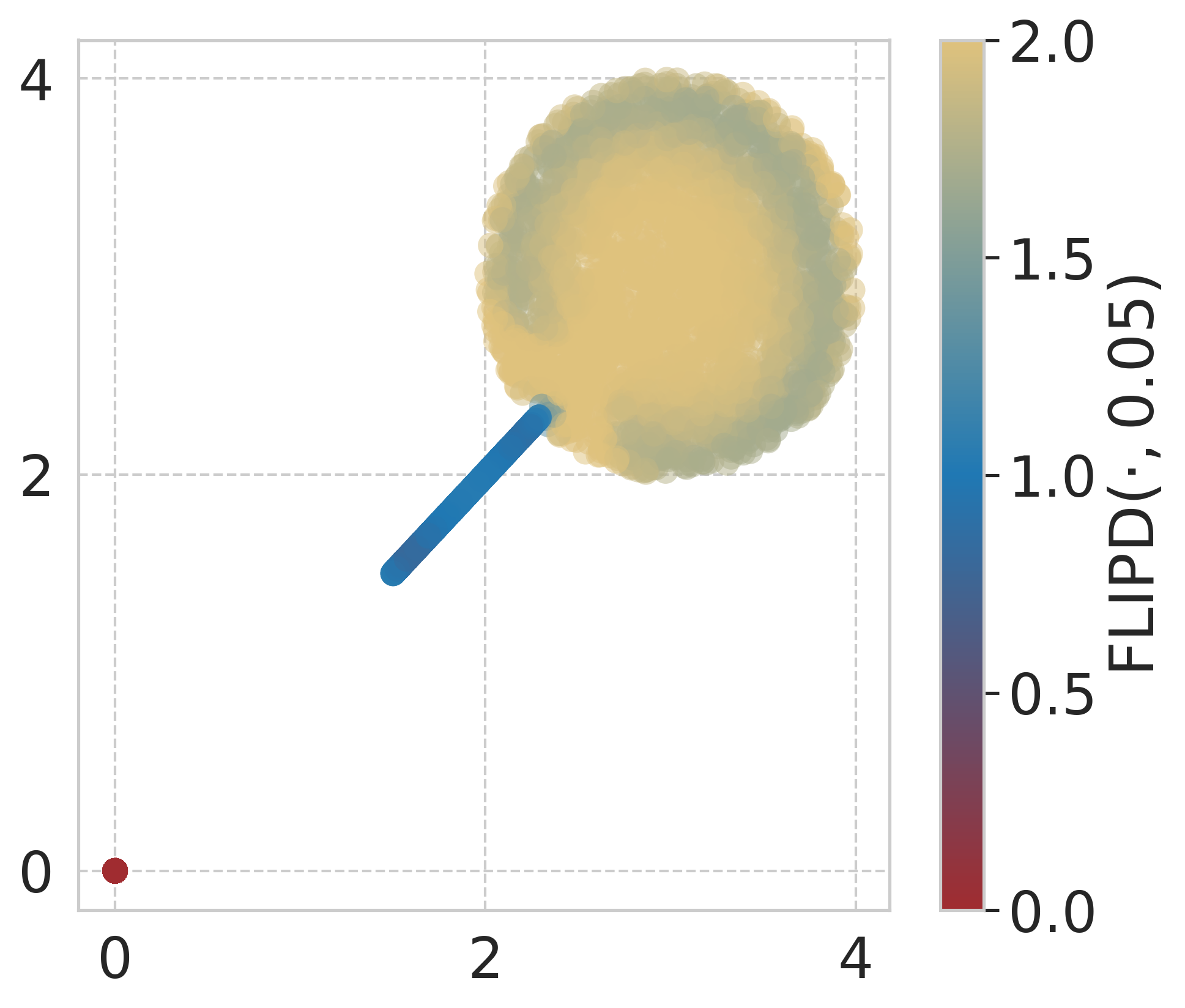
Figure 5: The FLIPD estimates on a Lollipop dataset from [60].

Figure 5 shows pointwise LID estimates for a “lollipop” distribution taken from [60]. It is a uniform distribution over three submanifolds: $(i)$ a 2d “candy”, $(ii)$ a 1d “stick”, and $(iii)$ an isolated point of zero dimensions. Note that the FLIPD estimates at $t_{0}=0.05$ for all three submanifolds are coherent.

Figure 6 shows the FLIPD curve as training progresses on the lollipop example and the Gaussian mixture that was already discussed in section 4. We see that gradually, knee patterns emerge at the correct LID, indicating that the DM is learning the data manifold. Notably, data with higher LID values get assigned higher estimates even after a few epochs, demonstrating that FLIPD effectively ranks data based on LID, even when the DM is underfitted.

Finally, Figure 7 presents a summary of complex manifolds obtained from neural spline flows and high-dimensional mixtures, showing knees around the true LID.

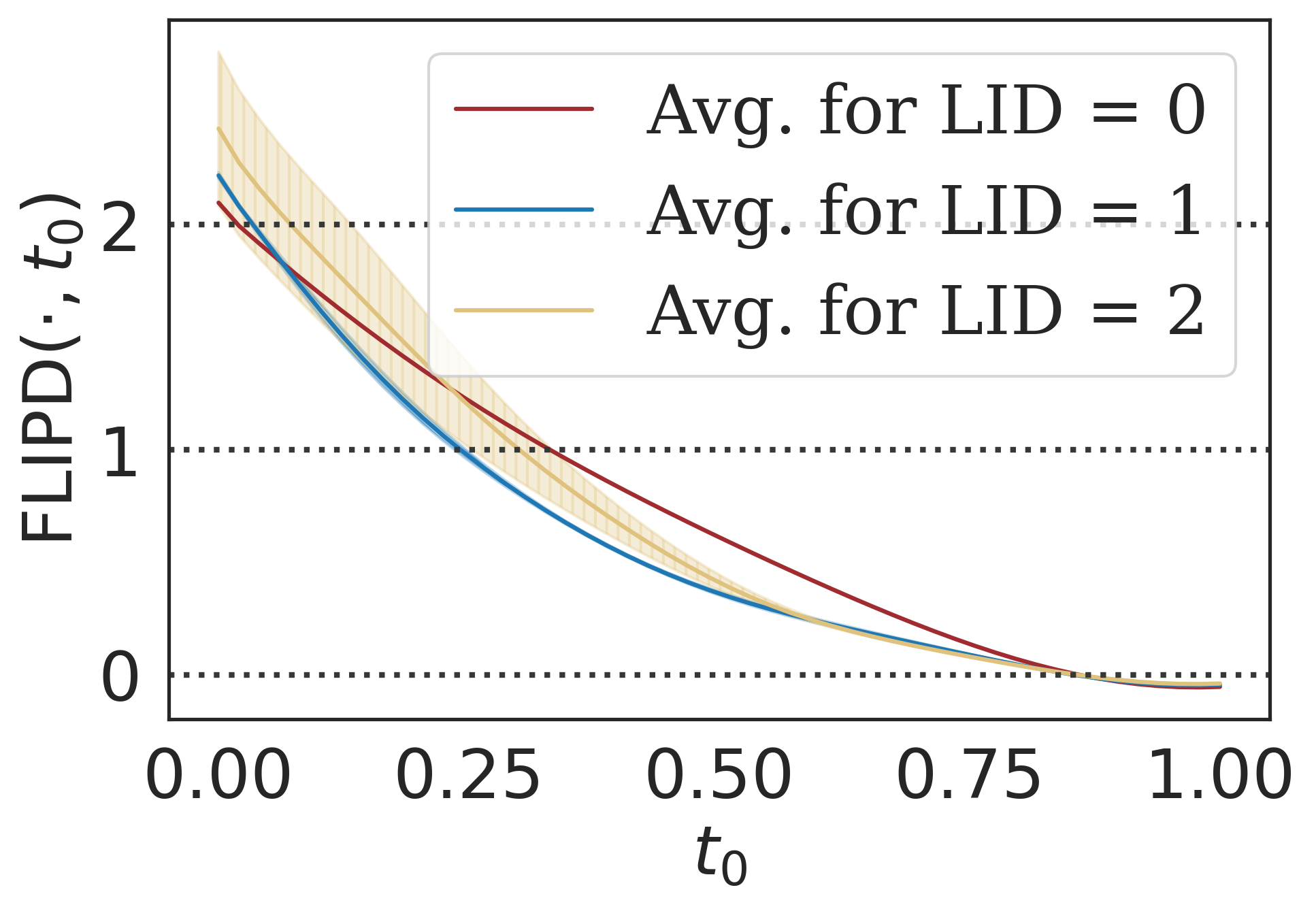
(a) After 10 epochs.

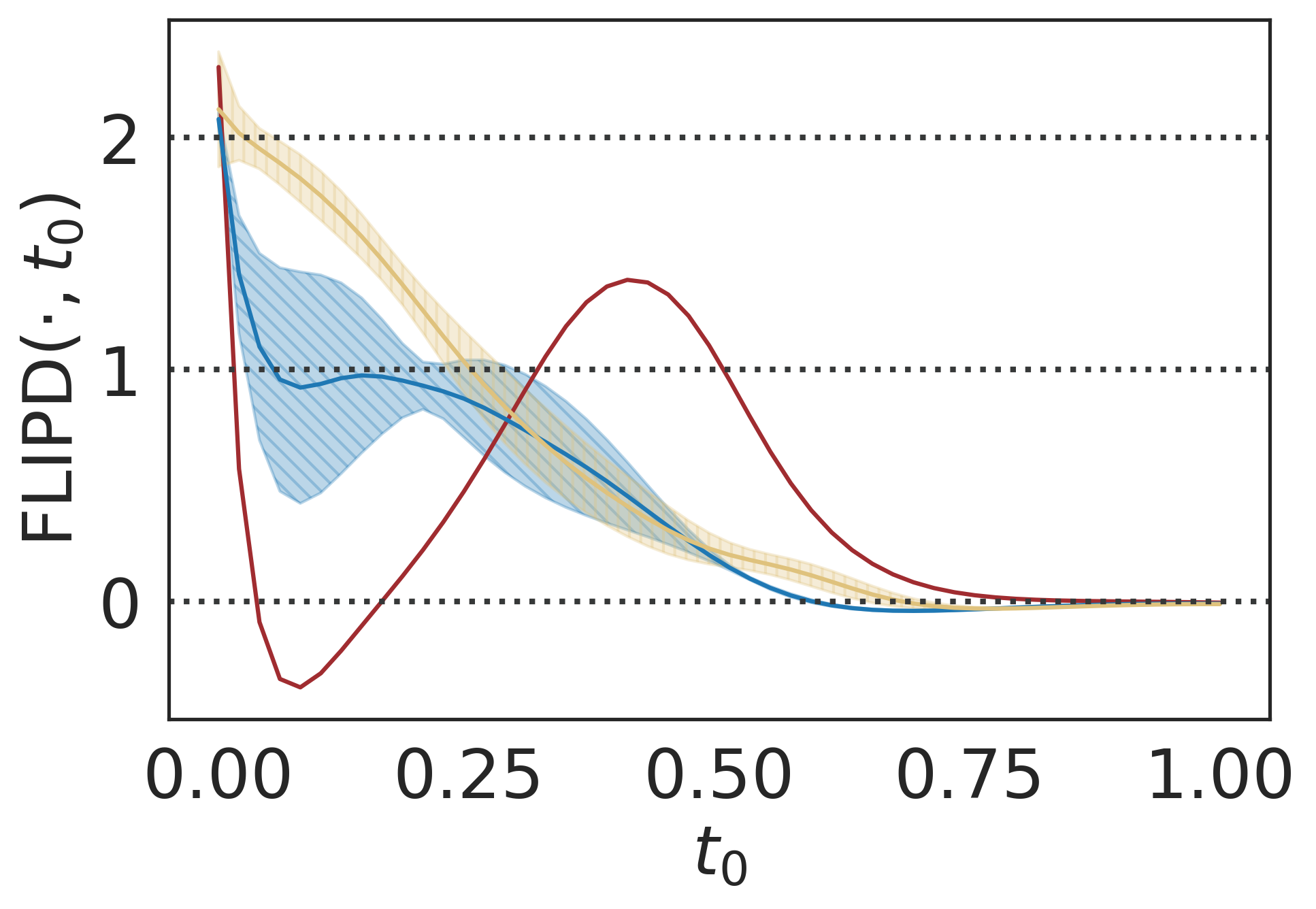
(b) After 20 epochs.

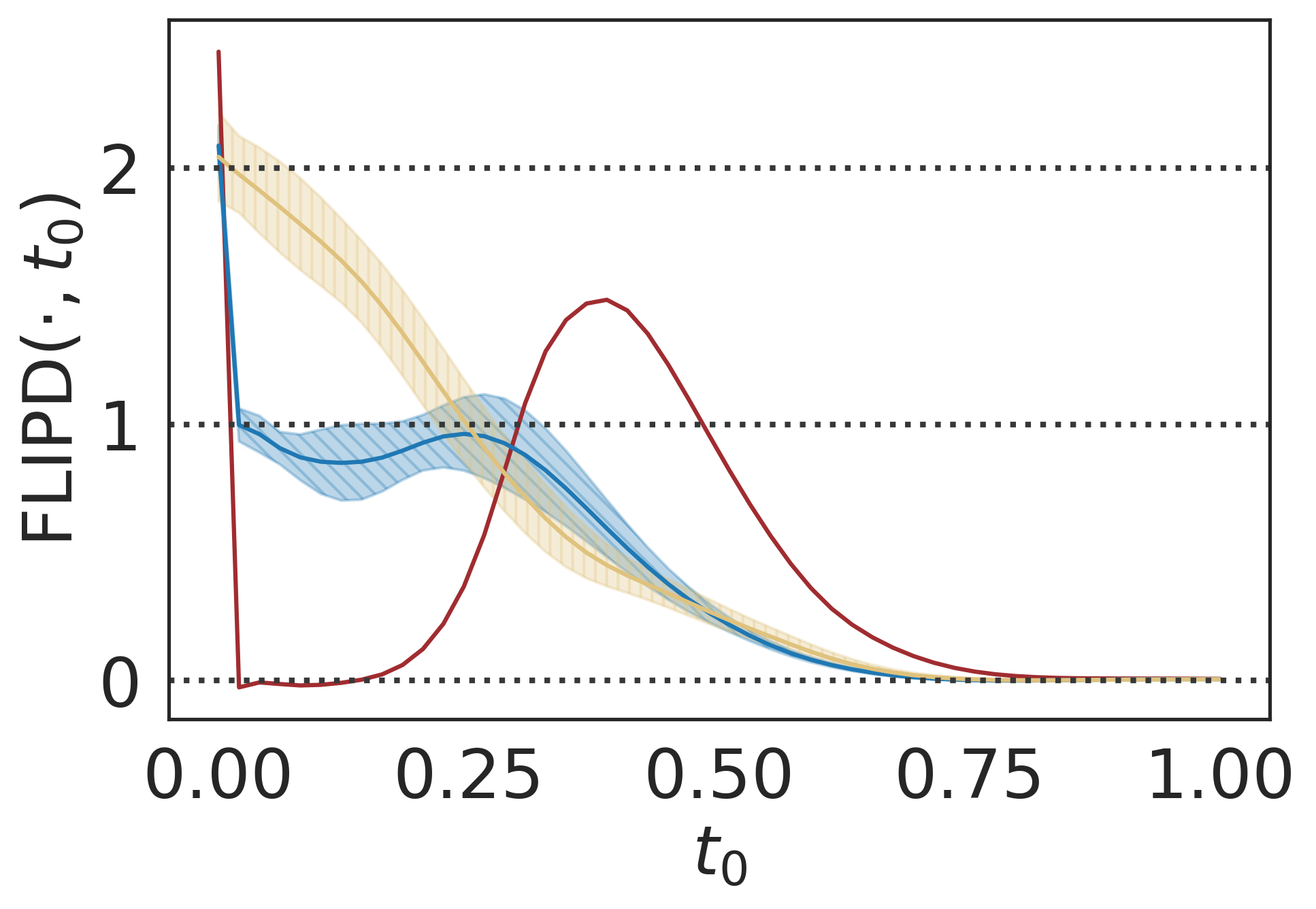
(c) After 100 epochs.

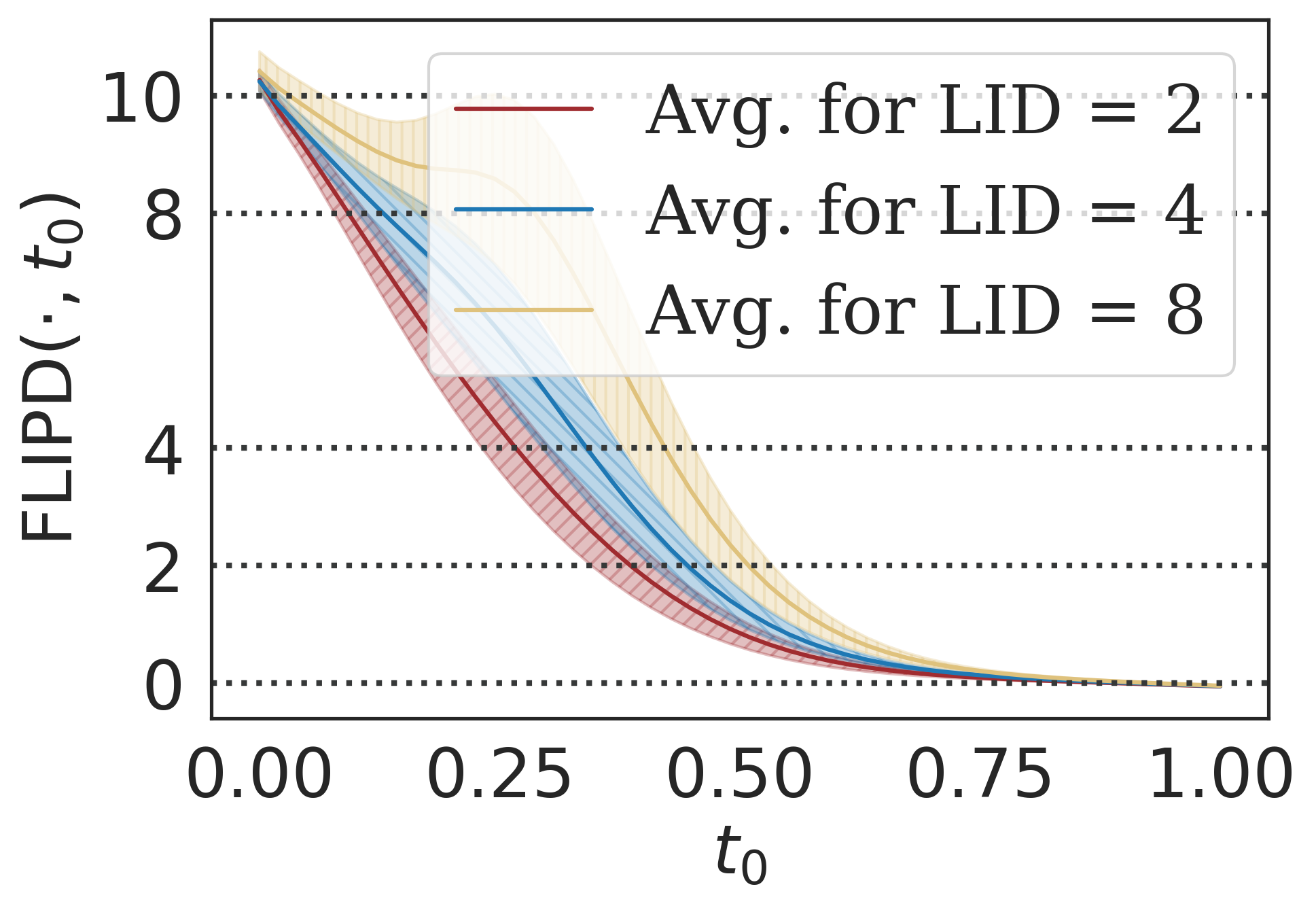
(d) After 10 epochs.

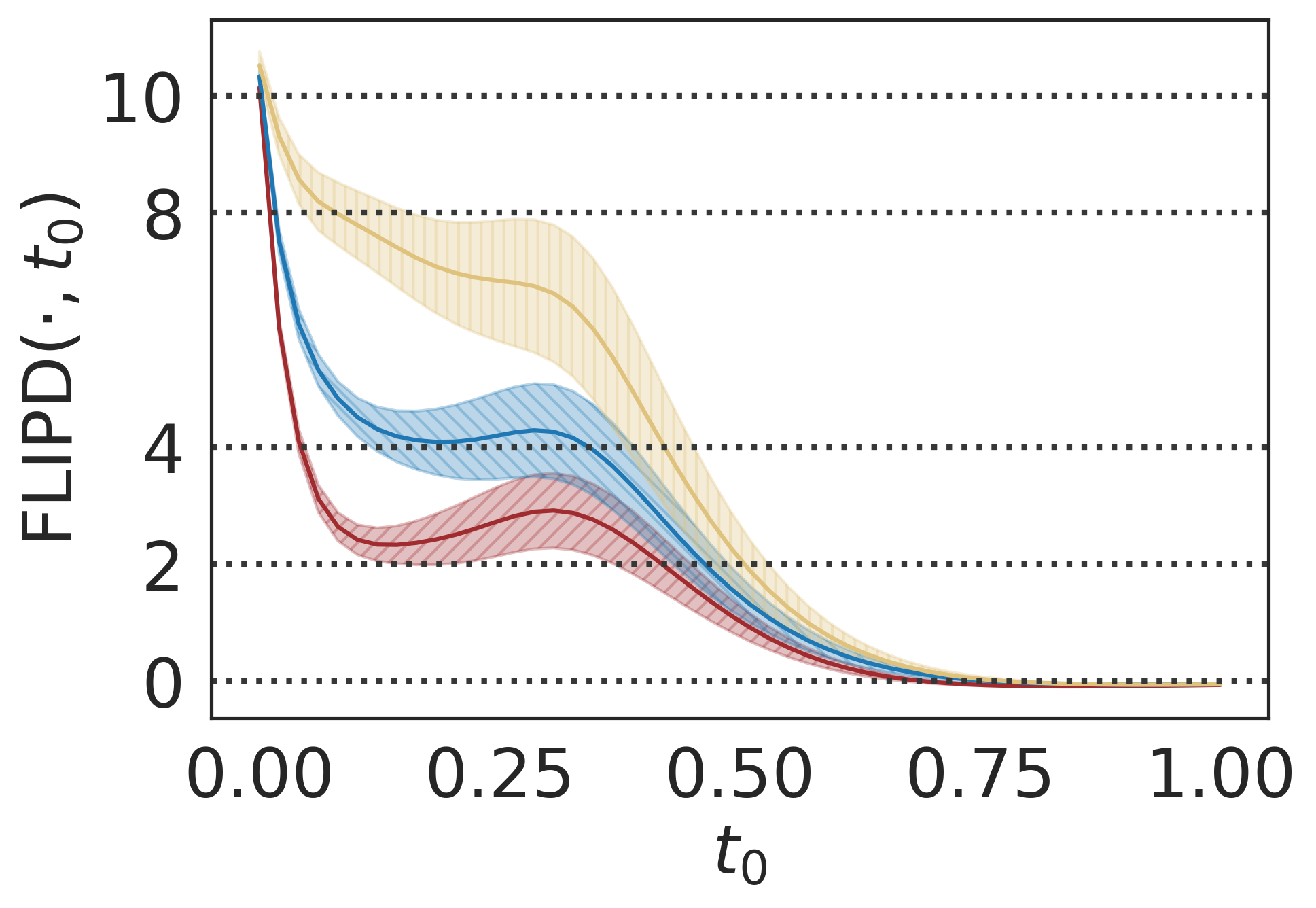
(e) After 20 epochs.

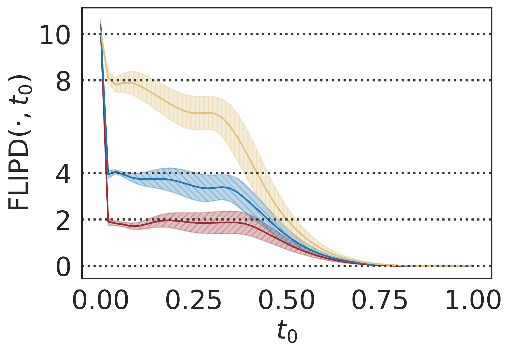
(f) After 100 epochs.

Figure 6: The evolution of the FLIPD curve while training the DM to fit a Lollipop (top) and a manifold mixture $\mathcal{N}_{2}+\mathcal{N}_{4}+\mathcal{N}_{8}\subseteq\mathbb{R}^{10}$ (bottom).

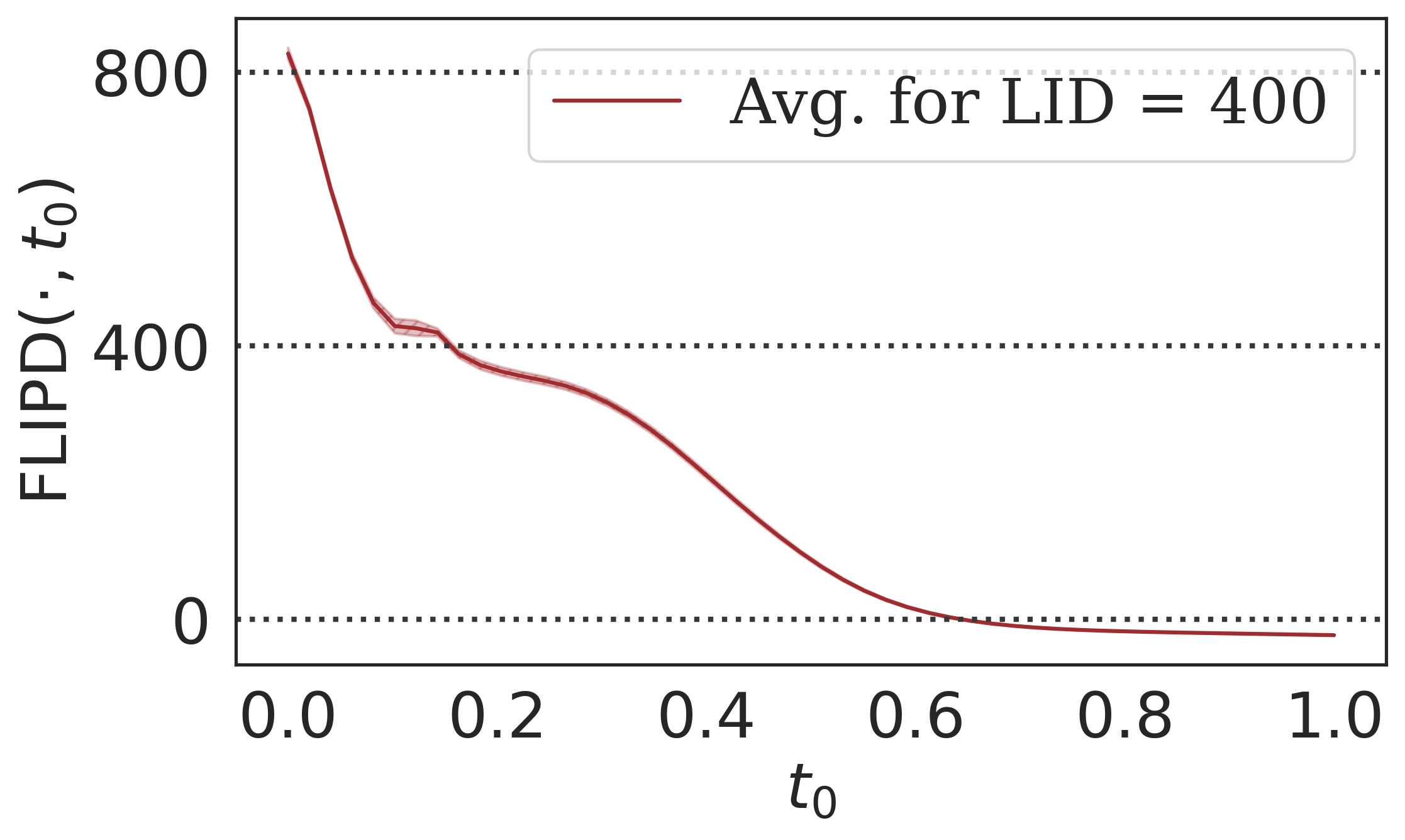
(a)   $\mathcal{F}_{400}\subseteq\mathbb{R}^{800}$.

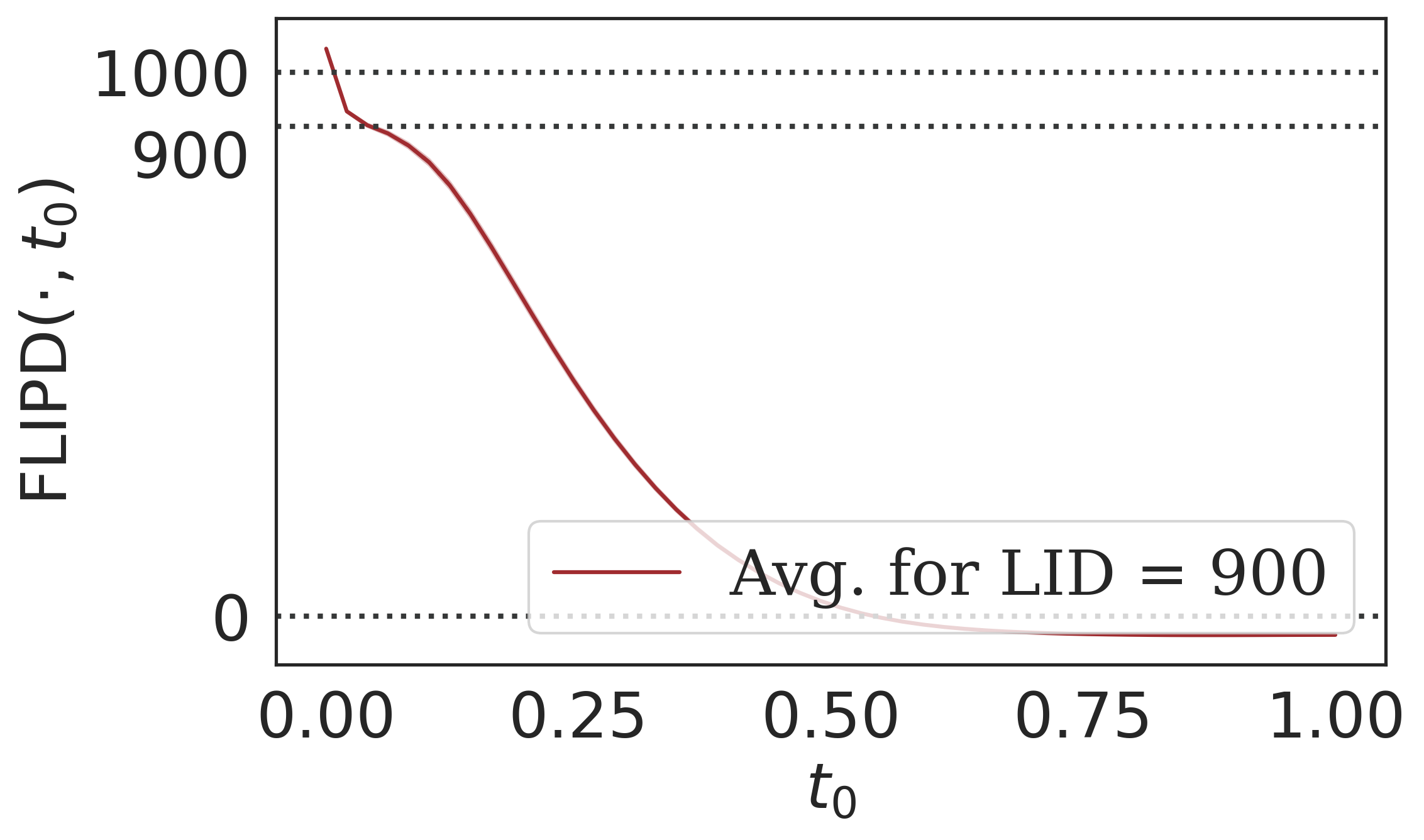
(b)   $\mathcal{U}_{900}\subseteq\mathbb{R}^{1000}$.

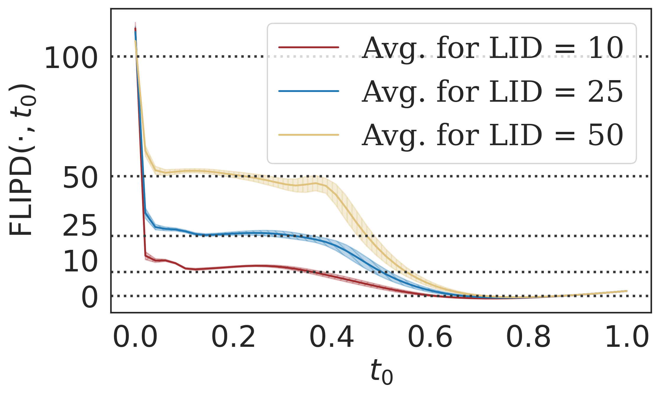
(c)   $\mathcal{N}_{10}+\mathcal{N}_{25}+\mathcal{N}_{50}\subseteq\mathbb{R}^{100}$.

Figure 7: The FLIPD curve for complex and high-dimensional manifolds.

D.3 A Simple Multiscale Experiment

Tempczyk et al. [60] argue that when setting $\delta$, all the directions of data variation that have a log standard deviation below $\delta$ are ignored. Here, we make this connection more explicit.

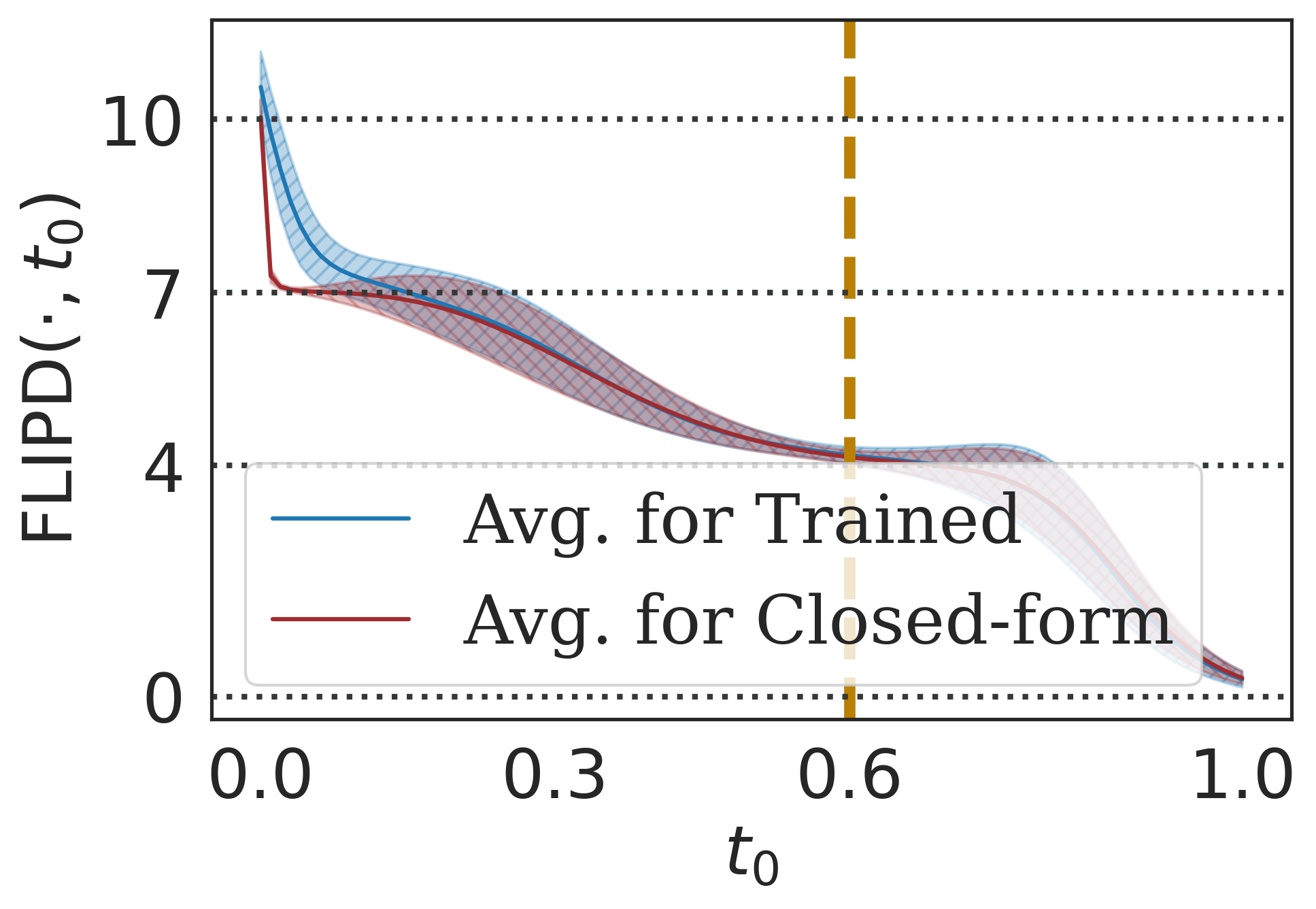
Figure 8: FLIPD curve for a multivariate Gaussian with controlled covariance eigenspectrum.

We define a multivariate Gaussian distribution with a prespecified eigenspectrum for its covariance matrix: having three eigenvalues of $10^{-4}$, three eigenvalues of $1$, and four eigenvalues of $10^{3}$. This ensures that the distribution is numerically 7d and that the directions and amount of data variation are controlled using the eigenvectors and eigenvalues of the covariance matrix.

For this multivariate Gaussian, the score function in Equation 13 can be written in closed form; thus, we evaluate FLIPD both with and without training a DM. We see in Figure 8 the estimates obtained in both scenarios match closely, with some deviations due to imperfect model fit, which we found matches perfectly when training for longer.

Apart from the initial knee at $7$, which is expected, we find another at $t_{0}=0.6$ (corresponding to $e^{\delta}\approx 6.178$ with our hyperparameter setup in Table 4) where the value of FLIPD is $4$. This indeed confirms that the estimator focuses solely on the 4d space characterized by the eigenvectors having eigenvalues of $10^{3}$, and by ignoring the eigenvalues $10^{-4}$ and $1$ which are both smaller than $6.178$.

D.4 In-depth Analysis of the Synthetic Benchmark

Generating Manifold Mixtures

To create synthetic data, we generate each component of our manifold mixture separately and then join them to form a distribution. All mixture components are sampled with equal probability in the final distribution. For a component with the intrinsic dimension of $d$, we first sample from a base distribution in $d$ dimensions. This base distribution is isotropic Gaussian and Laplace for $\mathcal{N}_{d}$ and $\mathcal{L}_{d}$ and uniform for the case of $\mathcal{U}_{d}$ and $\mathcal{F}_{d}$. We then zero-pad these samples to match the ambient dimension $D$ and perform a random $D\times D$ rotation on $\mathbb{R}^{D}$ (each component has one such transformation). For $\mathcal{F}_{d}$, we have an additional step to make the submanifold complex. We first initialize a neural spline flow (using the nflows library [18]) with 5 coupling transforms, 32 hidden layers, 32 hidden blocks, and tail bounds of 10. The data is then passed through the flow, resulting in a complex manifold embedded in $\mathbb{R}^{D}$ with an LID of $d$. Finally, we standardize each mixture component individually and set their modes such that the pairwise Euclidean distance between them is at least 20. We then translate each component so its barycenter matches the corresponding mode, ensuring that data from different components rarely mixes, thus maintaining distinct LIDs.

LIDL Baseline

Following the hyperparameter setup in [60], we train $8$ models with different noised-out versions of the dataset with standard deviations $e^{\delta_{i}}\in\{0.01,0.014,0.019,0.027,0.037,0.052,0.072,0.1\}$. The normalizing flow backbone is taken from [18], using 10 piecewise rational quadratic transforms with 32 hidden dimensions, 32 blocks, and a tail bound of 10. While [60] uses an autoregressive flow architecture, we use coupling transforms for increased training efficiency and to match the training time of a single DM.

Setup

We use model-free estimators from the skdim library [5] and across our experiments, we sample $10^{6}$ points from the synthetic distributions for either fitting generative models or fitting the model-free estimators. We then evaluate LID estimates on a uniformly subsampled set of $2^{12}$ points from the original set of $10^{6}$ points. Some methods are relatively slow, and this allows us to have a fair, yet feasible comparison. We do not see a significant difference even when we double the size of the subsampled set. We focus on four different model-free baselines for our evaluation: ESS [29], LPCA [21, 11], MLE [37, 42], and FIS [1]. We use default settings throughout, except for high-dimensional cases ($D>100$), where we set the number of nearest neighbours $k$ to $1000$ instead of the default $100$. This adjustment is necessary because we observed a significant performance drop, particularly in LPCA, when $k$ was too small in these scenarios. We note that this adjustment has not been previously implemented in similar benchmarks conducted by Tempczyk et al. [60], despite their claim that their method outperforms model-free alternatives. We also note that FIS does not scale beyond $100$ dimensions, and thus leave it blank in our reports. Computing pairwise distances on high dimensions ($D\geq 800$) on all $10^{6}$ samples takes over 24 hours even with $40$ CPU cores. Therefore, for $D\geq 800$, we use the same $2^{12}$ subsamples we use for evaluation.

Evaluation

We have three tables to summarize our analysis: $(i)$ Table 6 shows the MAE of the LID estimates, comparing each datapoint’s estimate to the ground truth at a fine-grained level; $(ii)$ Table 8 shows the average LID estimate for synthetic manifolds with only one component, this average is typically used to estimate global intrinsic dimensionality in baselines; finally, $(iii)$ Table 7 looks at the concordance index [22] of estimates for cases with multiple submanifolds of different dimensionalities. Concordance indices for a sequence of estimates $\{\widehat{\text{LID}}\}_{n=1}^{N}$ are defined as follows:

$$\mathcal{C}\left(\{\text{LID}_{n}\}_{n=1}^{N},\{\widehat{\text{LID}}_{n}\}_{n=1}^{N}\right)=\sum_{\begin{subarray}{c}1\leq n_{1}\neq n_{2}\leq N\\ \text{LID}_{n_{1}}\leq\text{LID}_{n_{2}}\end{subarray}}\mathbb{I}(\widehat{\text{LID}}_{n_{1}}\leq\widehat{\text{LID}}_{n_{2}})/\binom{N}{2},$$ (78)

where $\mathbb{I}$ is the indicator function; a perfect estimator will have a $\mathcal{C}$ of $1$. Instead of emphasizing the actual values of the LID estimates, this metric assesses how well the ranks of an estimator align with those of ground truth [58, 44, 59, 30], thus evaluating LID as a “relative” measure of complexity.

Model-free Analysis

Among model-free methods, LPCA and ESS show good performance in low dimensions, with LPCA being exceptionally good in scenarios where the manifold is affine. As we see in Table 6, while model-free methods produce reliable estimates when $D$ is small, as $D$ increases the estimates become more unreliable. In addition, we include average LID estimates in Table 8 and see that all model-free baselines underestimate intrinsic dimensionality to some degree, with LPCA and MLE being particularly drastic when $D>100$. We note that ESS performs relatively well, even beating model-based methods in some $800$-dimensional scenarios. However, we note that both the $\mathcal{C}$ values in Table 7 and MAE values in Tables 6 and 8 suggest that none of these estimators effectively estimate LID in a pointwise manner and cannot rank data by LID as effectively as FLIPD.

Model-based Analysis

Focusing on model-based methods, we see in Table 7 that all except FLIPD perform poorly in ranking data based on LID. Remarkably, FLIPD achieves perfect $\mathcal{C}$ values among all datasets; further justifying it as a relative measure of complexity. We also note that while LIDL and NB provide better global estimates in Table 8 for high dimensions, they have worse MAE performance in Table 6. This once again suggests that at a local level, our estimator is superior compared to others, beating all baselines in $4$ out of $5$ groups of synthetic manifolds in Table 6.

D.5 Ablations

We begin by evaluating the impact of using kneedle. Our findings, summarized in Table 5, indicate that while setting a small fixed $t_{0}$ is effective in low dimensions, the advantage of kneedle becomes particularly evident as the number of dimensions increases.

We also tried combining it with kneedle by sweeping over the origin $\delta_{1}$ and arguing that the estimates obtained from this method also exhibit knees. Despite some improvement in high-dimensional settings, Table 5 shows that even coupling it with kneedle does not help.

Table 5: MAE (lower is better). Rows show synthetic manifolds and columns represent different variations of our Fokker-Planck-based estimators.

Synthetic Manifold	FLIPD	FLIPD	FPRegress	FPRegress
	$t_{0}\!=\!.05$	kneedle	kneedle	$\delta_{1}\!=\!-1$
Lollipop in $\mathbb{R}^{2}$	$\mathbf{0.142}$	$0.419$	$0.572$	$0.162$
String within doughnut $\mathbb{R}^{3}$	$\mathbf{0.052}$	$0.055$	$0.398$	$0.377$
Swiss Roll in $\mathbb{R}^{3}$	$\mathbf{0.053}$	$0.055$	$0.087$	$0.161$
$\mathcal{L}_{5}\subseteq\mathbb{R}^{10}$	$\mathbf{0.100}$	$0.169$	$1.168$	$0.455$
$\mathcal{N}_{90}\subseteq\mathbb{R}^{100}$	$0.501$	$\mathbf{0.492}$	$3.142$	$0.998$
$\mathcal{U}_{10}+\mathcal{U}_{30}+\mathcal{U}_{90}\subseteq\mathbb{R}^{100}$	$3.140$	$\mathbf{1.298}$	$5.608$	$10.617$
$\mathcal{F}_{10}+\mathcal{F}_{25}+\mathcal{F}_{50}\subseteq\mathbb{R}^{100}$	$14.37$	$\mathbf{3.925}$	$16.32$	$21.01$
$\mathcal{U}_{10}+\mathcal{U}_{80}+\mathcal{U}_{200}\subseteq\mathbb{R}^{800}$	$39.54$	$\mathbf{14.30}$	$30.06$	$29.99$

D.6 Improving the NB Estimators with kneedle

We recall that the NB estimator requires computing $\operatorname{rank}S(x)$, where $S(x)$ is a $K\times D$ matrix formed by stacking the scores $\hat{s}(\cdot,t_{0})$. We set $t_{0}=0.01$ as it provides the most reasonable estimates. To compute $\operatorname{rank}S(x)$ numerically, Stanczuk et al. [57] perform a singular value decomposition on $S(x)$ and use a cutoff threshold $\tau$ below which singular values are considered zero. Finding the best $\tau$ is challenging, so Stanczuk et al. [57] propose finding the two consecutive singular values with the maximum gap. Furthermore, we see that sometimes the top few singular values are disproportionately higher than the rest, resulting in severe overestimations of the LID. Thus, we introduce an alternative algorithm to determine the optimal $\tau$. For each $\tau$, we estimate LID by thresholding the singular values. Sweeping 100 different $\tau$ values from 0 to $1000$ at a geometric scale (to further emphasize smaller thresholds) produces estimates ranging from $D$ (keeping all singular values) to 0 (ignoring all). As $\tau$ varies, we see that the estimates plateau over a certain range of $\tau$. We use kneedle to detect this plateau because the starting point of a plateau is indeed a knee in the curve. This significantly improves the baseline, especially in high dimensions: see the third column of Tables 6, 8, and 7 compared to the second column.

Table 6: MAE (lower is better). Each row represents a synthetic dataset and each column represents an LID estimation method. Rows are split into groups based on the ambient dimension: the first group of rows shows toy examples; the second shows low-dimensional data with $D=10$; the third shows moderate-dimensional data with $D=100$; and the last two show high-dimensional data with $D=800$ and $D=1000$, respectively.

	Model-based				Model-free
Synthetic Manifold	FLIPD kneedle	NB Vanilla	NB kneedle	LIDL	ESS	LPCA	MLE	FIS
Lollipop $\subseteq\mathbb{R}^{2}$	$0.419$	$0.577$	$0.855$	$\mathbf{0.052}$	$0.009$	$\mathbf{0.000}$	$0.142$	$0.094$
Swiss Roll $\subseteq\mathbb{R}^{3}$	$0.055$	$0.998$	$\mathbf{0.016}$	$0.532$	$0.017$	$\mathbf{0.000}$	$0.165$	$0.018$
String within doughnut $\subseteq\mathbb{R}^{3}$	$\mathbf{0.055}$	$1.475$	$0.414$	$1.104$	$0.017$	$\mathbf{0.000}$	$0.128$	$0.041$
Summary (Toy Manifolds)	$\mathbf{0.176}$	$1.017$	$0.428$	$0.563$	$0.014$	$\mathbf{0.000}$	$0.145$	$0.051$
$\mathcal{N}_{5}\subseteq\mathbb{R}^{10}$	$0.084$	$5.000$	$\mathbf{0.005}$	$0.071$	$0.061$	$\mathbf{0.000}$	$0.441$	$0.206$
$\mathcal{L}_{5}\subseteq\mathbb{R}^{10}$	$0.169$	$1.000$	$0.146$	$\mathbf{0.101}$	$0.068$	$\mathbf{0.000}$	$0.462$	$0.203$
$\mathcal{U}_{5}\subseteq\mathbb{R}^{10}$	$0.324$	$4.994$	$0.933$	$\mathbf{0.123}$	$0.153$	$\mathbf{0.000}$	$0.451$	$0.186$
$\mathcal{F}_{5}\subseteq\mathbb{R}^{10}$	$0.666$	$1.216$	$0.765$	$\mathbf{0.487}$	$0.168$	$\mathbf{0.000}$	$0.497$	$0.176$
$\mathcal{N}_{2}+\mathcal{N}_{4}+\mathcal{N}_{8}\subseteq\mathbb{R}^{10}$	$\mathbf{0.287}$	$5.706$	$1.078$	$0.308$	$0.156$	$\mathbf{0.000}$	$0.406$	$0.206$
$\mathcal{L}_{2}+\mathcal{L}_{4}+\mathcal{L}_{8}\subseteq\mathbb{R}^{10}$	$\mathbf{0.253}$	$5.708$	$0.772$	$0.515$	$0.193$	$\mathbf{0.001}$	$0.437$	$0.018$
$\mathcal{U}_{2}+\mathcal{U}_{4}+\mathcal{U}_{8}\subseteq\mathbb{R}^{10}$	$0.586$	$5.677$	$3.685$	$\mathbf{0.363}$	$0.331$	$\mathbf{0.115}$	$0.540$	$0.222$
$\mathcal{F}_{2}+\mathcal{F}_{4}+\mathcal{F}_{8}\subseteq\mathbb{R}^{10}$	$\mathbf{0.622}$	$5.709$	$2.187$	$1.013$	$0.428$	$\mathbf{0.115}$	$0.642$	$0.269$
Summary ($10$-dimensional)	$\mathbf{0.066}$	$0.381$	$0.161$	$0.211$	$0.005$	$\mathbf{0.000}$	$0.054$	$0.019$
$\mathcal{U}_{10}\subseteq\mathbb{R}^{100}$	$0.910$	$30.115$	$\mathbf{0.000}$	$1.370$	$0.644$	$\mathbf{0.000}$	$1.263$	$-$
$\mathcal{U}_{30}\subseteq\mathbb{R}^{100}$	$0.505$	$50.521$	$\mathbf{0.000}$	$0.542$	$1.465$	$\mathbf{0.002}$	$7.622$	$-$
$\mathcal{U}_{90}\subseteq\mathbb{R}^{100}$	$0.640$	$1.157$	$1.327$	$\mathbf{0.332}$	$\mathbf{2.034}$	$21.90$	$39.65$	$-$
$\mathcal{N}_{30}\subseteq\mathbb{R}^{100}$	$0.887$	$52.43$	$\mathbf{0.000}$	$0.892$	$0.534$	$\mathbf{0.000}$	$5.703$	$-$
$\mathcal{N}_{90}\subseteq\mathbb{R}^{100}$	$0.492$	$\mathbf{0.184}$	$2.693$	$0.329$	$\mathbf{1.673}$	$21.88$	$39.45$	$-$
$\mathcal{F}_{80}\subseteq\mathbb{R}^{100}$	$\mathbf{1.869}$	$20.00$	$3.441$	$1.871$	$\mathbf{3.660}$	$16.78$	$34.41$	$-$
$\mathcal{U}_{10}+\mathcal{U}_{25}+\mathcal{U}_{50}\subseteq\mathbb{R}^{100}$	$\mathbf{0.868}$	$57.96$	$0.890$	$5.869$	$\mathbf{4.988}$	$6.749$	$16.12$	$-$
$\mathcal{U}_{10}+\mathcal{U}_{30}+\mathcal{U}_{90}\subseteq\mathbb{R}^{100}$	$\mathbf{1.298}$	$61.58$	$1.482$	$8.460$	$21.89$	$\mathbf{20.06}$	$41.05$	$-$
$\mathcal{N}_{10}+\mathcal{N}_{25}+\mathcal{N}_{50}\subseteq\mathbb{R}^{100}$	$1.813$	$74.20$	$\mathbf{0.555}$	$8.873$	$7.712$	$\mathbf{5.716}$	$14.37$	$-$
$\mathcal{F}_{10}+\mathcal{F}_{25}+\mathcal{F}_{50}\subseteq\mathbb{R}^{100}$	$\mathbf{3.925}$	$74.20$	$6.205$	$18.61$	$9.200$	$\mathbf{6.769}$	$16.78$	$-$
Summary ($100$-dimensional)	$\mathbf{1.321}$	$42.24$	$1.659$	$4.715$	$\mathbf{5.380}$	$9.986$	$21.64$	$-$
$\mathcal{U}_{200}\subseteq\mathbb{R}^{800}$	$11.54$	$600.0$	$\mathbf{7.205}$	$55.98$	$3.184$	$\mathbf{0.000}$	$159.3$	$-$
$\mathcal{F}_{400}\subseteq\mathbb{R}^{800}$	$20.46$	$400.0$	$\mathbf{10.15}$	$207.2$	$14.48$	$\mathbf{2.919}$	$342.6$	$-$
$\mathcal{U}_{10}+\mathcal{U}_{80}+\mathcal{U}_{200}\subseteq\mathbb{R}^{800}$	$\mathbf{14.30}$	$715.3$	$18.82$	$120.7$	$1.385$	$\mathbf{0.004}$	$72.25$	$-$
Summary ($800$-dimensional)	$15.43$	$571.8$	$\mathbf{12.06}$	$128.0$	$6.350$	$\mathbf{0.974}$	$191.4$	-
$\mathcal{N}_{900}\subseteq\mathbb{R}^{1000}$	$\mathbf{3.913}$	$100.0$	$24.38$	$10.45$	$\mathbf{14.16}$	$219.8$	$819.2$	$-$
$\mathcal{U}_{100}\subseteq\mathbb{R}^{1000}$	$12.81$	$900.0$	$62.68$	$\mathbf{12.65}$	$1.623$	$\mathbf{0.000}$	$72.06$	$-$
$\mathcal{U}_{900}\subseteq\mathbb{R}^{1000}$	$12.81$	$100.0$	$\mathbf{0.104}$	$24.90$	$\mathbf{14.49}$	$219.1$	$810.2$	$-$
$\mathcal{F}_{500}\subseteq\mathbb{R}^{1000}$	$\mathbf{21.77}$	$500.0$	$52.19$	$341.3$	$\mathbf{18.83}$	$29.99$	$435.7$	$-$
Summary ($1000$-dimensional)	$\mathbf{12.83}$	$400.0$	$34.84$	$97.33$	$\mathbf{12.28}$	$117.2$	$534.3$	$-$

Table 7: Concordance index (higher is better with $1.000$ being the gold standard). Each row represents a mixture of multi-dimensional manifolds, and each column represents an LID estimation method. This table evaluates how accurately different estimators rank datapoints based on their LID.

Synthetic Manifold	FLIPD kneedle	NB Vanilla	NB kneedle	LIDL	ESS	LPCA	MLE	FIS
Lollipop $\subseteq\mathbb{R}^{2}$	$\mathbf{1.000}$	$0.426$	$0.394$	$0.999$	$\mathbf{1.000}$	$\mathbf{1.000}$	$\mathbf{1.000}$	$\mathbf{1.000}$
String withing doughnut $\subseteq\mathbb{R}^{3}$	$\mathbf{1.000}$	$0.483$	$0.486$	$0.565$	$\mathbf{1.000}$	$\mathbf{1.000}$	$\mathbf{1.000}$	$\mathbf{1.000}$
$\mathcal{N}_{2}+\mathcal{N}_{4}+\mathcal{N}_{8}\subseteq\mathbb{R}^{10}$	$\mathbf{1.000}$	$0.341$	$0.725$	$0.943$	$\mathbf{1.000}$	$\mathbf{1.000}$	$\mathbf{1.000}$	$\mathbf{1.000}$
$\mathcal{L}_{2}+\mathcal{L}_{4}+\mathcal{L}_{8}\subseteq\mathbb{R}^{10}$	$\mathbf{1.000}$	$0.342$	$0.752$	$0.884$	$\mathbf{1.000}$	$\mathbf{1.000}$	$\mathbf{1.000}$	$\mathbf{1.000}$
$\mathcal{U}_{2}+\mathcal{U}_{4}+\mathcal{U}_{8}\subseteq\mathbb{R}^{10}$	$\mathbf{1.000}$	$0.334$	$0.462$	$0.903$	$\mathbf{1.000}$	$\mathbf{1.000}$	$\mathbf{1.000}$	$\mathbf{1.000}$
$\mathcal{F}_{2}+\mathcal{F}_{4}+\mathcal{F}_{8}\subseteq\mathbb{R}^{10}$	$\mathbf{1.000}$	$0.342$	$0.578$	$0.867$	$\mathbf{1.000}$	$\mathbf{1.000}$	$0.999$	$\mathbf{1.000}$
$\mathcal{U}_{10}+\mathcal{U}_{25}+\mathcal{U}_{50}\subseteq\mathbb{R}^{100}$	$\mathbf{1.000}$	$0.467$	$0.879$	$0.759$	$0.855$	$0.897$	$\mathbf{1.000}$	$-$
$\mathcal{U}_{10}+\mathcal{U}_{30}+\mathcal{U}_{90}\subseteq\mathbb{R}^{100}$	$\mathbf{1.000}$	$0.342$	$0.826$	$0.742$	$0.742$	$0.855$	$\mathbf{1.000}$	$-$
$\mathcal{N}_{10}+\mathcal{N}_{25}+\mathcal{N}_{50}\subseteq\mathbb{R}^{100}$	$\mathbf{1.000}$	$0.342$	$0.866$	$0.736$	$0.878$	$0.917$	$\mathbf{1.000}$	$-$
$\mathcal{F}_{10}+\mathcal{F}_{25}+\mathcal{F}_{50}\subseteq\mathbb{R}^{100}$	$\mathbf{1.000}$	$0.342$	$0.731$	$0.695$	$0.847$	$0.897$	$\mathbf{1.000}$	$-$
$\mathcal{U}_{10}+\mathcal{U}_{80}+\mathcal{U}_{200}\subseteq\mathbb{R}^{800}$	$\mathbf{1.000}$	$0.342$	$0.841$	$0.697$	$\mathbf{1.000}$	$\mathbf{1.000}$	$\mathbf{1.000}$	$-$

Table 8: Analysis on manifolds with a single global intrinsic dimension. Columns, categorized by whether or not they use a model, display various LID estimators. The first set of rows shows the average LID as a global intrinsic dimension estimate and is grouped into lower- $(D\leq 100)$ or higher-dimensional $(D>100)$ categories. Methods that most closely match the true intrinsic dimension are bolded. The second set of rows shows the pointwise precision of the estimators, as indicated by MAE (lower is better): while previous baselines generally provide reliable global estimates, their pointwise precision is subpar, especially with higher dimensionality.

	Model-based				Model-free
	FLIPD kneedle	NB Vanilla	NB kneedle	LIDL	ESS	LPCA	MLE	FIS
Synthetic Manifold	Average LID Estimate
Swiss Roll $\subseteq\mathbb{R}^{3}$	$\mathbf{2.012}$	$2.998$	$1.984$	$2.527$	$2.008$	$\mathbf{2.000}$	$2.013$	$2.003$
$\mathcal{N}_{5}\subseteq\mathbb{R}^{10}$	$5.017$	$10.00$	$\mathbf{4.995}$	$5.067$	$5.004$	$\mathbf{5.000}$	$5.108$	$5.187$
$\mathcal{L}_{5}\subseteq\mathbb{R}^{10}$	$\mathbf{4.968}$	$6.000$	$4.854$	$5.089$	$4.985$	$\mathbf{5.000}$	$5.123$	$5.182$
$\mathcal{U}_{5}\subseteq\mathbb{R}^{10}$	$4.796$	$9.994$	$4.067$	$\mathbf{5.107}$	$4.880$	$\mathbf{5.000}$	$4.833$	$5.152$
$\mathcal{F}_{5}\subseteq\mathbb{R}^{10}$	$\mathbf{4.722}$	$6.216$	$4.461$	$5.482$	$4.890$	$\mathbf{5.000}$	$4.829$	$5.131$
$\mathcal{U}_{10}\subseteq\mathbb{R}^{100}$	$11.68$	$40.12$	$\mathbf{10.00}$	$11.29$	$9.361$	$\mathbf{10.00}$	$8.905$	$-$
$\mathcal{U}_{30}\subseteq\mathbb{R}^{100}$	$31.01$	$80.52$	$\mathbf{30.00}$	$30.08$	$28.54$	$\mathbf{29.99}$	$22.38$	$-$
$\mathcal{U}_{90}\subseteq\mathbb{R}^{100}$	$89.54$	$91.16$	$91.32$	$\mathbf{90.24}$	$\mathbf{88.27}$	$68.10$	$50.35$	$-$
$\mathcal{N}_{30}\subseteq\mathbb{R}^{100}$	$30.79$	$82.43$	$\mathbf{30.00}$	$30.85$	$29.67$	$\mathbf{30.00}$	$24.38$	$-$
$\mathcal{N}_{90}\subseteq\mathbb{R}^{100}$	$\mathbf{89.88}$	$90.18$	$92.62$	$90.21$	$\mathbf{88.89}$	$68.12$	$50.55$	$-$
$\mathcal{F}_{80}\subseteq\mathbb{R}^{100}$	$77.97$	$100.0$	$83.23$	$\mathbf{81.46}$	$\mathbf{76.35}$	$63.22$	$45.59$	$-$
$\mathcal{U}_{200}\subseteq\mathbb{R}^{800}$	$211.5$	$800.0$	$\mathbf{207.2}$	$256.0$	$199.3$	$\mathbf{200.0}$	$40.73$	$-$
$\mathcal{F}_{400}\subseteq\mathbb{R}^{800}$	$454.7$	$800.0$	$\mathbf{410.1}$	$607.2$	$385.8$	$\mathbf{397.1}$	$57.37$	$-$
$\mathcal{N}_{900}\subseteq\mathbb{R}^{1000}$	$\mathbf{890.3}$	$1000.$	$924.4$	$924.4$	$\mathbf{897.3}$	$680.2$	$80.78$	$-$
$\mathcal{U}_{100}\subseteq\mathbb{R}^{1000}$	$135.76$	$1000.$	$162.7$	$\mathbf{112.6}$	$99.54$	$\mathbf{100.0}$	$27.94$	$-$
$\mathcal{U}_{900}\subseteq\mathbb{R}^{1000}$	$864.9$	$1000.$	$\mathbf{900.1}$	$911.9$	$\mathbf{899.3}$	$680.9$	$89.80$	$-$
$\mathcal{F}_{500}\subseteq\mathbb{R}^{1000}$	$582.7$	$1000.$	$\mathbf{552.2}$	$841.3$	$\mathbf{481.4}$	$470.0$	$64.29$	$-$
Manifolds Summary	Pointwise MAE Averaged Across Tasks
$\subseteq\mathbb{R}^{D}$ where $D\leq 100$	$0.633$	$15.20$	$0.924$	$\mathbf{0.561}$	$0.954$	$\mathbf{5.506}$	$11.83$	$-$
$\subseteq\mathbb{R}^{D}$ where $D>100$	$\mathbf{13.88}$	$433.3$	$26.12$	$108.7$	$\mathbf{11.13}$	$78.64$	$439.8$	$-$

Appendix E Image Experiments

E.1 FLIPD Curves and DM Samples

Figures 9 and 10 show DM-generated samples and the associated LID curves for $4096$ samples from the datasets. In Figure 10, the FLIPD curves with MLPs, which have clearly discernible knees as predicted by the theory, are more reasonable than those generated with UNets. The fact that FLIPD estimates are worse for UNets is surprising given that MLPs produce worse-looking samples, as shown in Figure 9. However, comparing the first and second rows of Figure 9, it also becomes clear that MLP-generated images still match some characteristics of the true dataset, suggesting that they may still be capturing the image manifold in useful ways. To explain the surprisingly poor FLIPD estimates of UNets, we hypothesize that the convolutional layers in the UNet provide some inductive biases which, while helpful to produce visually pleasing images, might also encourage the network to over-fixate on high-frequency features which are not visually perceptible. For example, Kirichenko et al. [33] showed how normalizing flows over-fixate on these features, and how this can cause them to assign large likelihoods to out-of-distribution data, even when the model produces visually convincing samples. We hypothesize that a similar underlying phenomenon might be at play here, and that DMs with UNets might be over-emphasizing “high-frequency” directions of variation in their LID estimates, even if they learn the semantic ones and thus produce pleasing images. However, an exploration of this hypothesis is outside the scope of our work, and we highlight once again that FLIPD remains a useful measure of complexity when using UNets.

E.2 UNet Architecture

We use UNet architectures from diffusers [65], mirroring the DM setup in Table 4 except for the score backbone. For greyscale images, we use a convolutional block and two attention-based downsampling blocks with channel sizes of $128$, $256$, and $256$. For colour images, we use two convolutional downsampling blocks (each with $128$ channels) followed by two attention downsampling blocks (each with $256$ channels). Both setups are mirrored with their upsampling counterparts.

E.3 Images Sorted by FLIPD

Figures 11, 12, 13, and 14 show $4096$ samples of CIFAR10, SVHN, MNIST, and FMNIST sorted according to their FLIPD estimate, showing a gradient transition from the least complex datapoints (e.g., the digit $1$ in MNIST) to the most complex ones (e.g., the digit $8$ in MNIST). We use MLPs for greyscales and UNets for colour images but see similar trends when switching between backbones.

E.4 How Many Hutchinson Samples are Needed?

Figure 15 compares the Spearman’s rank correlation coefficient between FLIPD while we use $k\in\{1,50\}$ Hutchinson samples vs. computing the trace deterministically with $D$ Jacobian-vector-products: $(i)$ Hutchinson sampling is particularly well-suited for UNet backbones, having higher correlations compared to their MLP counterparts; $(ii)$ as $t_{0}$ increases, the correlation becomes smaller, suggesting that the Hutchinson sample complexity increases at larger timescales; $(iii)$ for small $t_{0}$, even one Hutchinson sample is enough to estimate LID; $(iv)$ for the UNet backbone, $50$ Hutchinson samples are enough and have a high correlation (larger than $0.8$) even for $t_{0}$ as large as $0.5$.

E.5 More Analysis on Images

While we use $100$ nearest neighbours in Table 2 for ESS and LPCA, we tried both with $1000$ nearest neighbours and got similar results. Moreover, Figure 16 shows the correlation of FLIPD with PNG for $t_{0}\in(0,1)$, indicating a consistently high correlation at small $t_{0}$, and a general decrease while increasing $t_{0}$. Additionally, UNet backbones correlate better with PNG, likely because their convolutional layers capture local pixel differences and high-frequency features, aligning with PNG’s internal workings. However, high correlation is still seen when working with an MLP.

Figures 17, 19, 21, and 23 show images with smallest and largest FLIPD estimates at different values of $t_{0}$ for the UNet backbone and Figures 18, 20, 22, and 24 show the same for the MLP backbone: $(i)$ we see a clear difference in the complexity of top and bottom FLIPD estimates, especially for smaller $t_{0}$; this difference becomes less distinct as $t_{0}$ increases; $(ii)$ interestingly, even for larger $t_{0}$ values with smaller PNG correlations, we qualitatively observe a clustering of the most complex datapoints at the end; however, the characteristic of this clustering changes. For example, see Figures 17 at $t_{0}=0.3$, or 22 and 24 at $t_{0}=0.8$, suggesting that FLIPD focuses on coarse-grained measures of complexity at these scales; and finally $(iii)$ while MLP backbones underperform in sample generation, their orderings are more meaningful, even showing coherent visual clustering up to $t=0.8$ in all Figures 18, 20, 22, and 24; this is a surprising phenomenon that warrants future exploration.

E.6 Stable Diffusion

To test FLIPD with Stable Diffusion v1.5 [49], which is finetuned on a subset of LAION-Aesthetics, we sampled 1600 images from LAION-Aesthetics-650k and computed FLIPD scores for each.

We ran FLIPD with $t_{0}\in\{0.01,0.1,0.3,0.8\}$ and a single Hutchinson trace sample. In all cases, FLIPD ranking clearly corresponded to complexity, though we decided upon $t_{0}=0.3$ as best capturing the “semantic complexity” of image contents. All 1600 images for $t=0.3$ are depicted in Figure 25. For all timesteps, we show previews of the 8 lowest- and highest-LID images in Figure 26. Note that LAION is essentially a collection of URLs, and some are outdated. For the comparisons in Figure 26 and 4(c), we remove placeholder icons or blank images, which likely correspond to images that, at the time of writing this paper, have been removed from their respective URLs and which are generally given among the lowest LIDs.

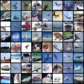
(a) CIFAR10 with UNet backbone.

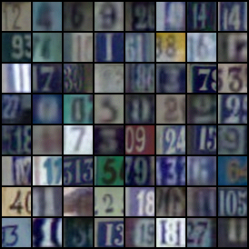
(b) SVHN with UNet backbone.

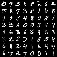
(c) MNIST with UNet backbone.

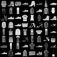
(d) FMNIST with UNet backbone.

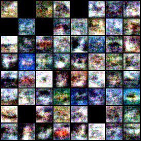
(e) CIFAR10 with MLP backbone.

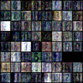
(f) SVHN with MLP backbone.

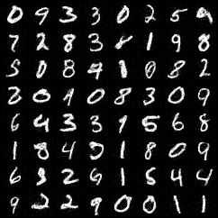
(g) MNIST with MLP backbone.

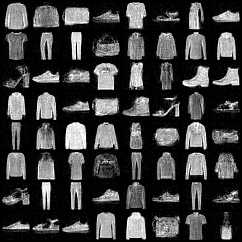
(h) FMNIST with MLP backbone.

Figure 9: Samples generated from DMs with different score network backbones, using the same seed for control. Despite the variation in backbones, images of the same cell in the grid (comparing top and bottom rows) show rough similarities, especially on CIFAR10 and SVHN.

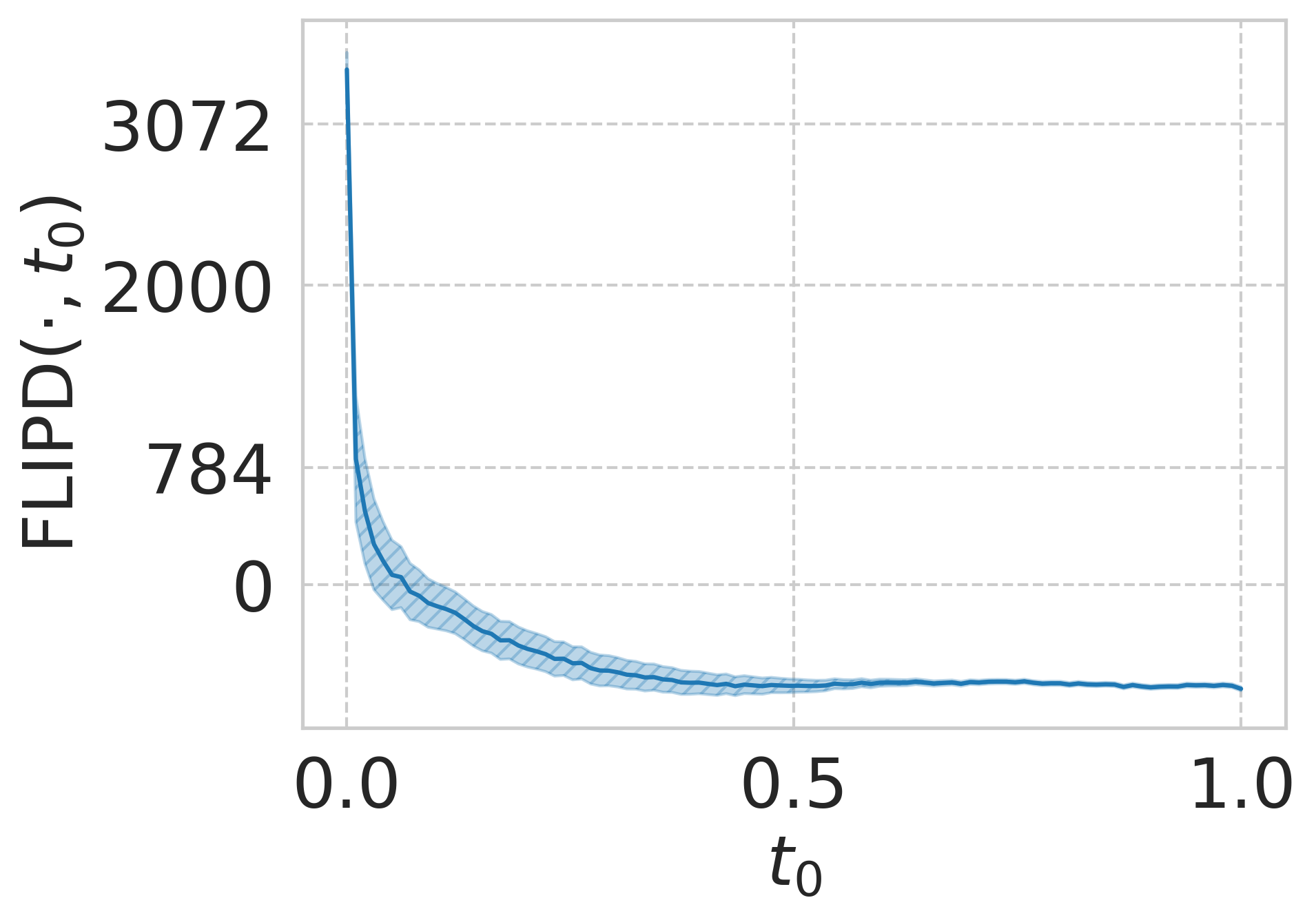
(a) CIFAR10 with UNet backbone.

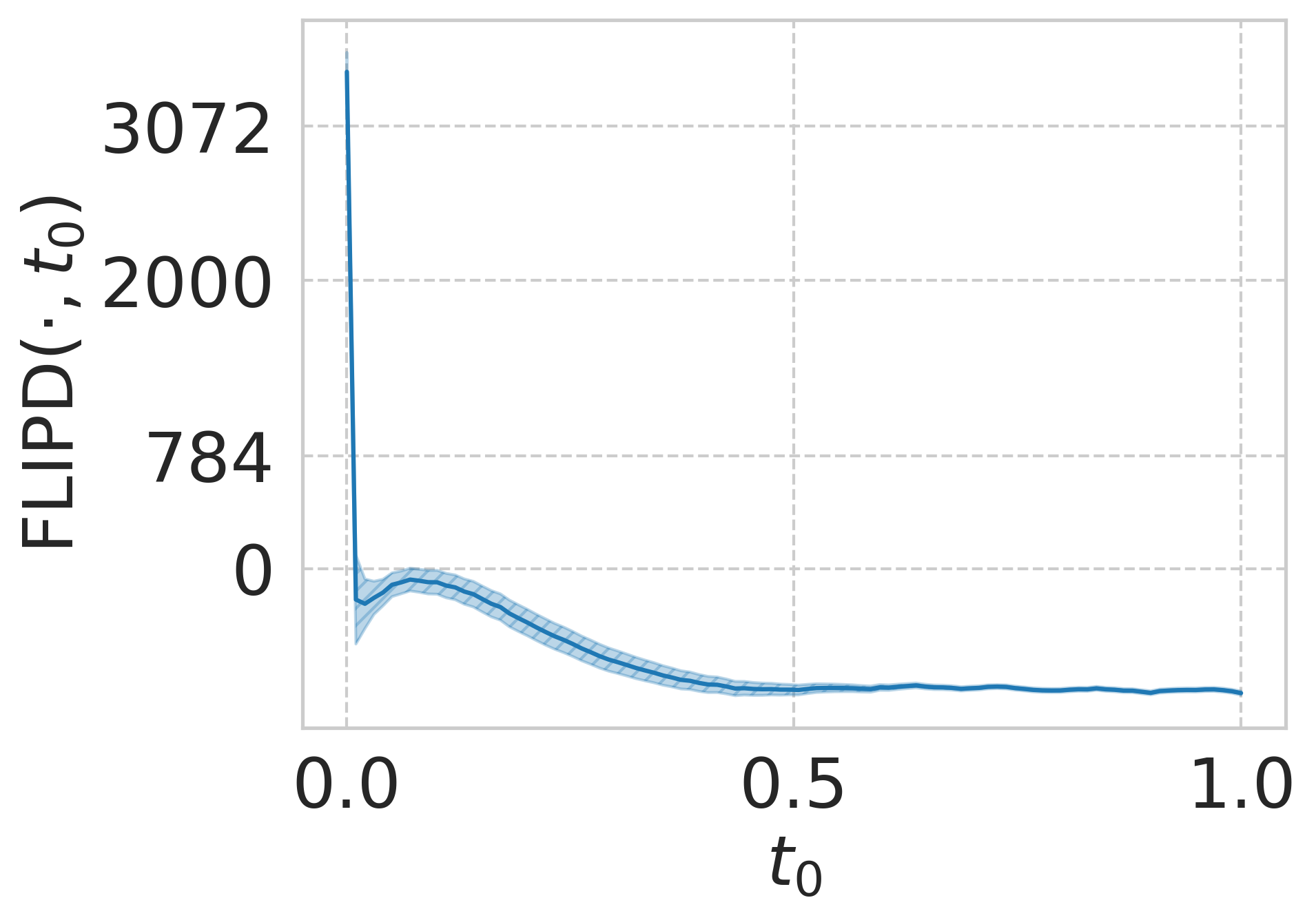
(b) SVHN with UNet backbone.

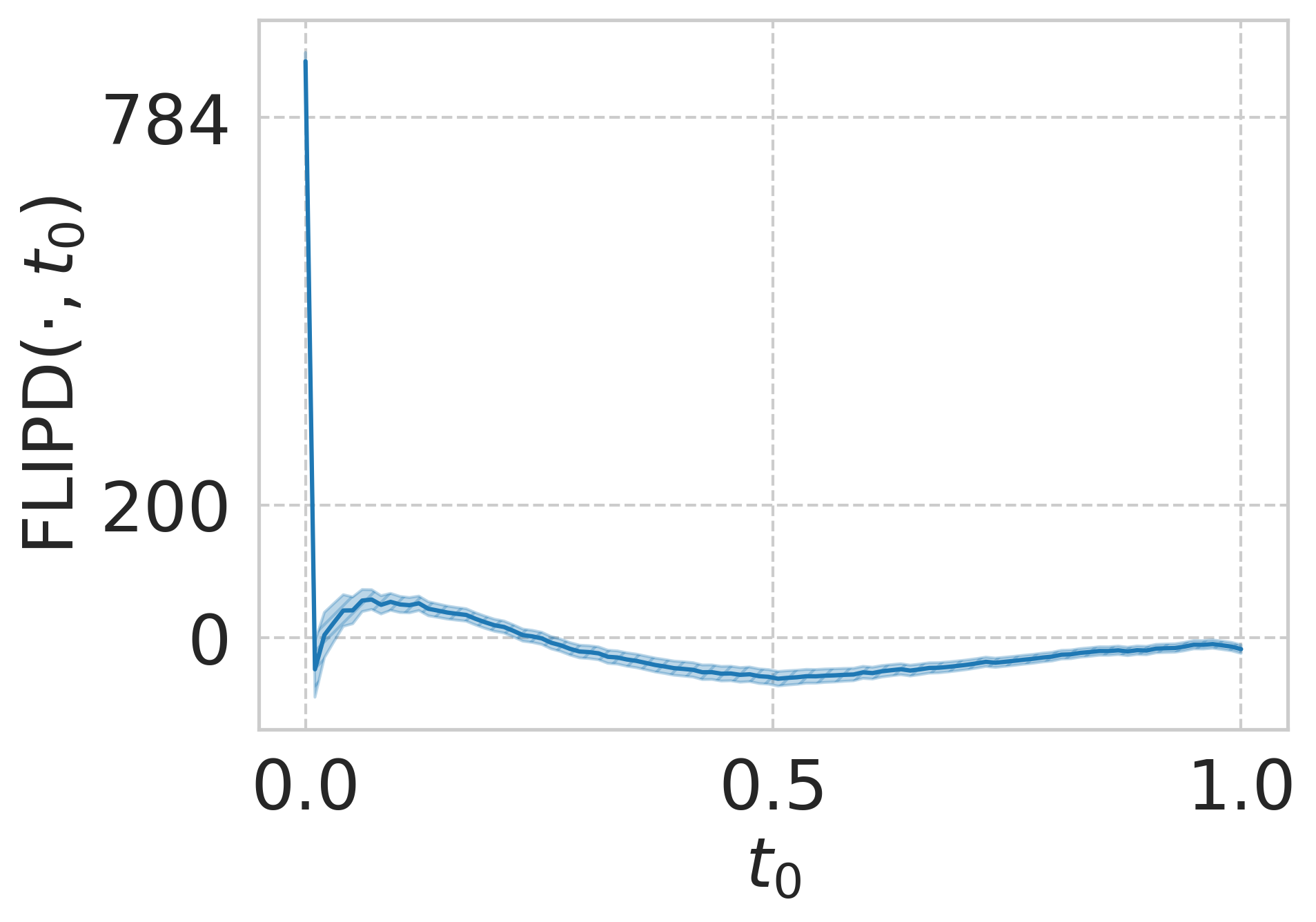
(c) MNIST with UNet backbone.

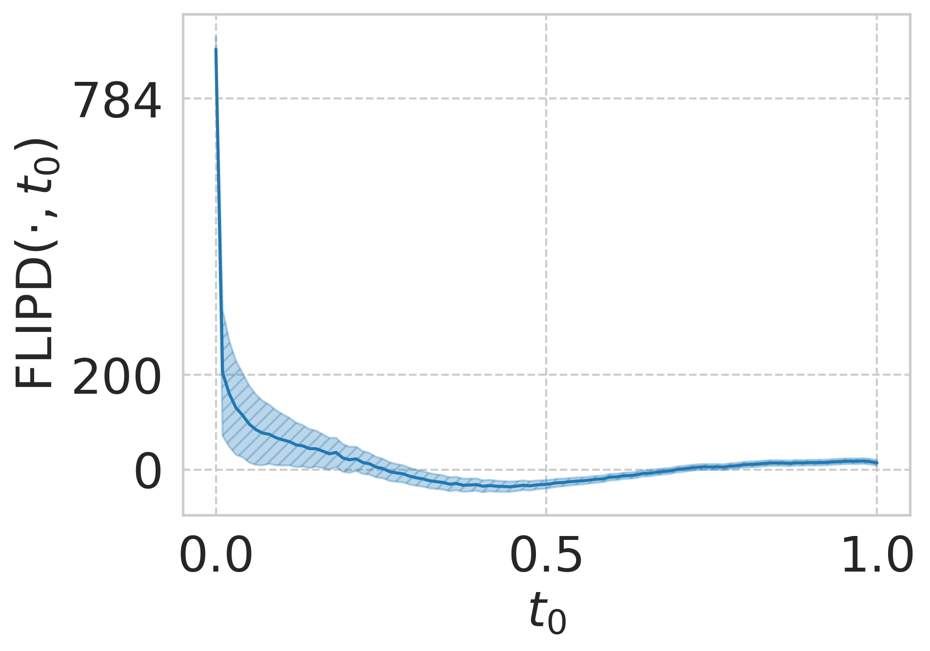
(d) FMNIST with UNet backbone.

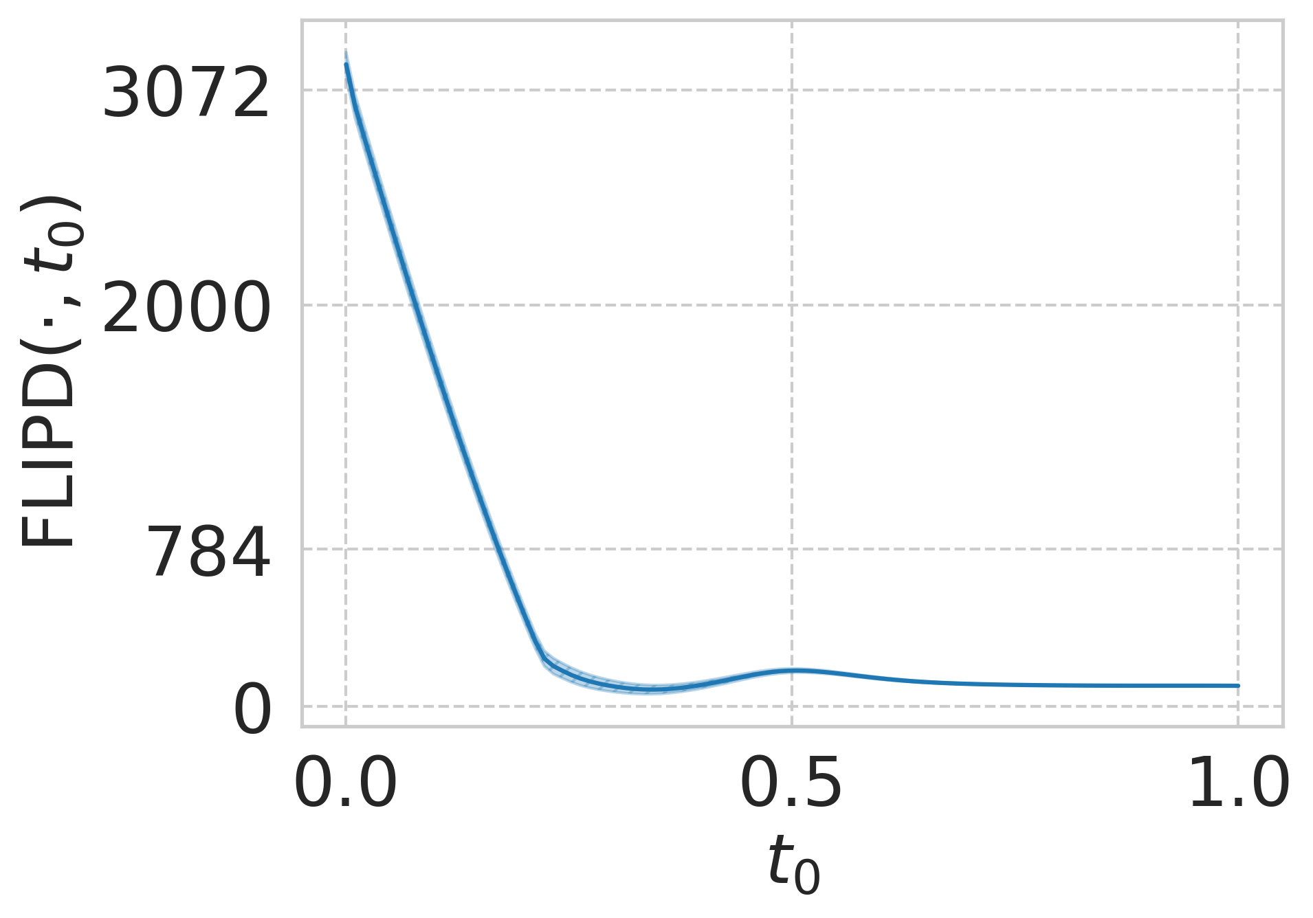
(e) CIFAR10 with MLP backbone.

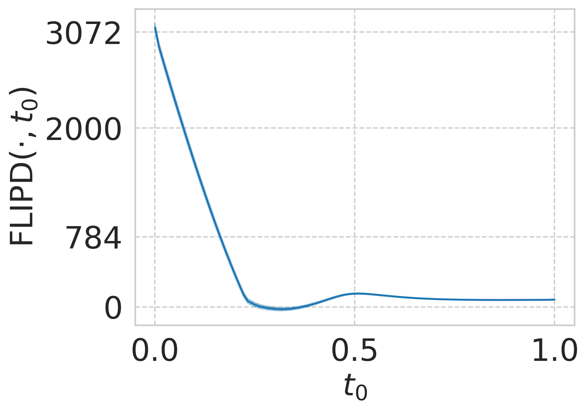
(f) SVHN with MLP backbone.

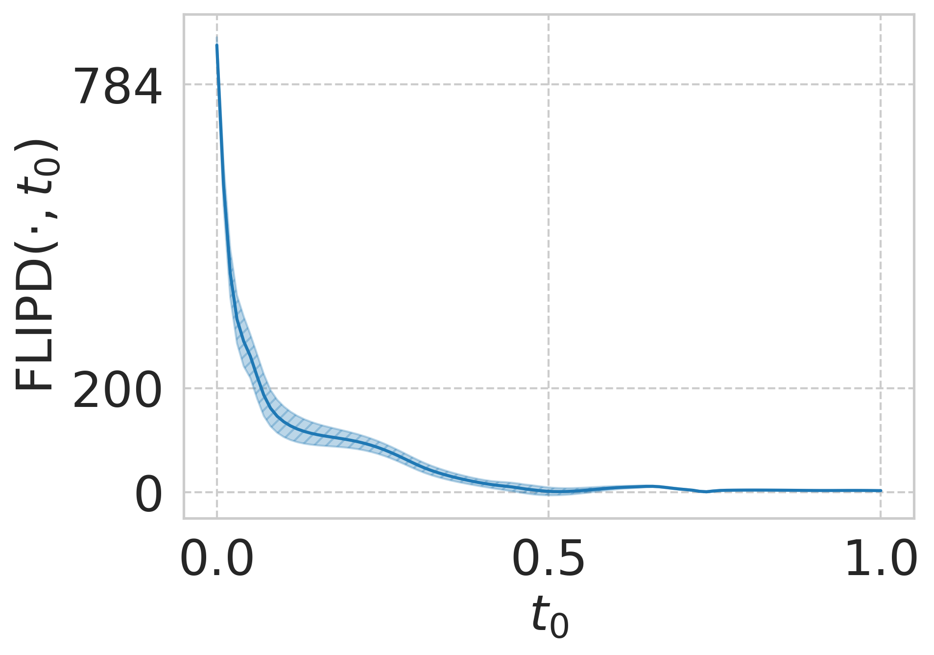
(g) MNIST with MLP backbone.

(h) FMNIST with MLP backbone.

Figure 10: FLIPD curves from all the different DMs with different score network backbones.

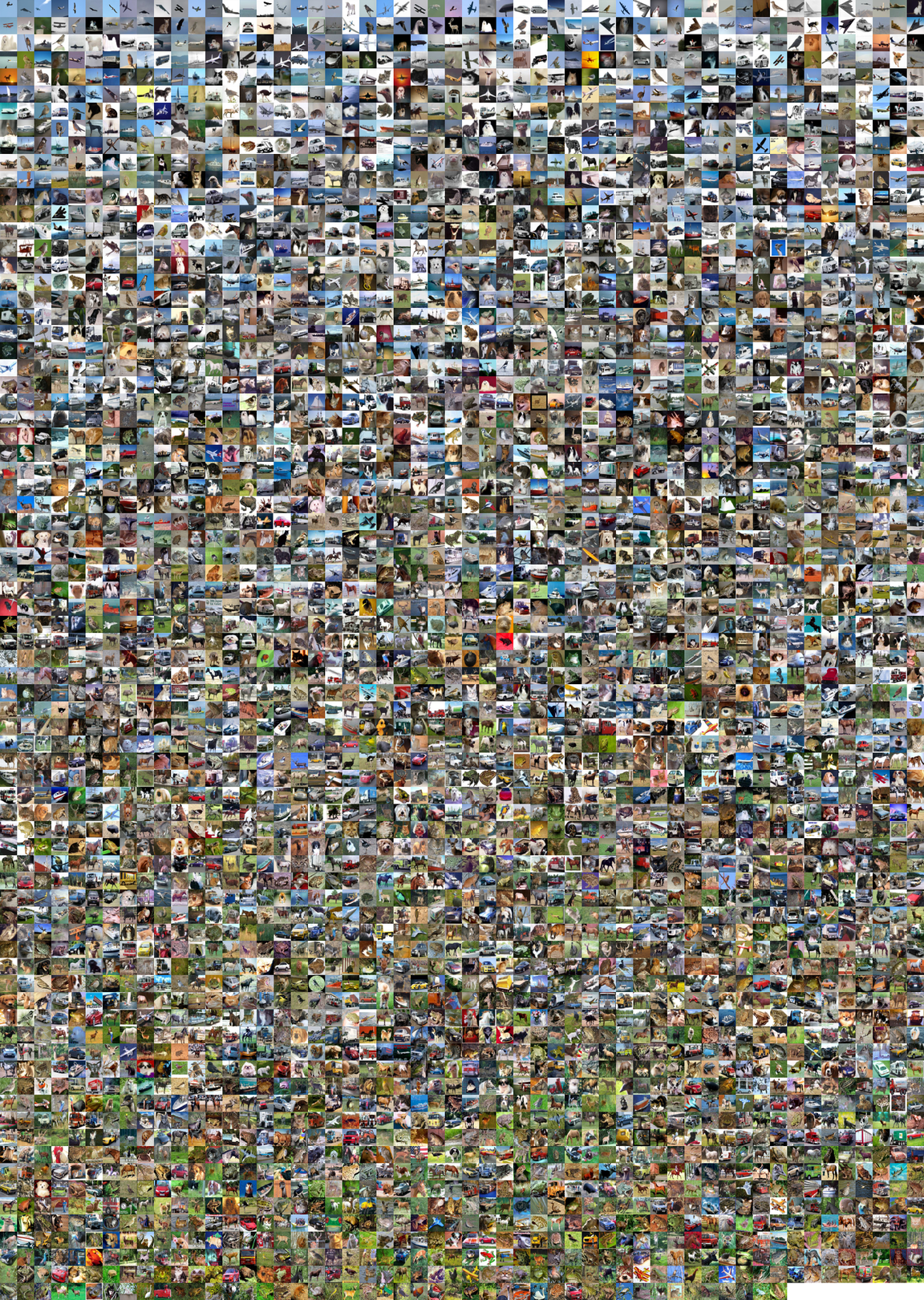
Figure 11: CIFAR10 sorted (left to right and top to bottom) by FLIPD estimate (UNet) at $t_{0}=0.01$.

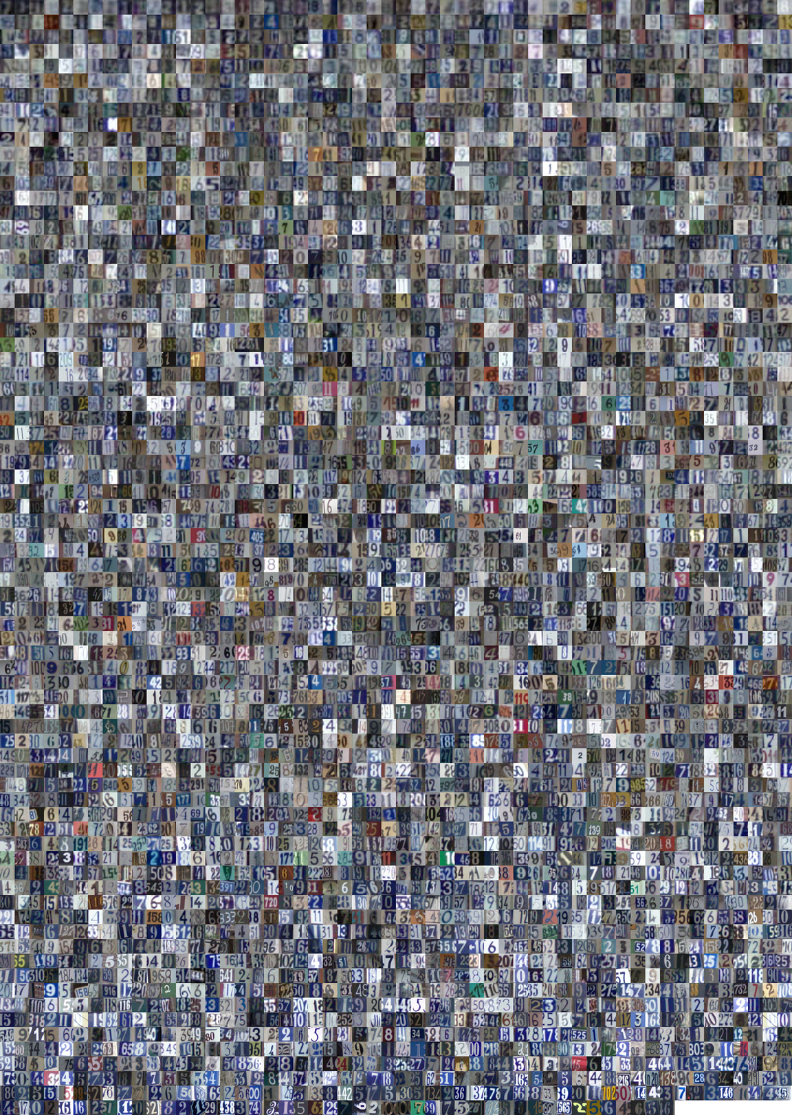
Figure 12: SVHN sorted (left to right and top to bottom) by FLIPD estimate (UNet) at $t_{0}=0.01$.

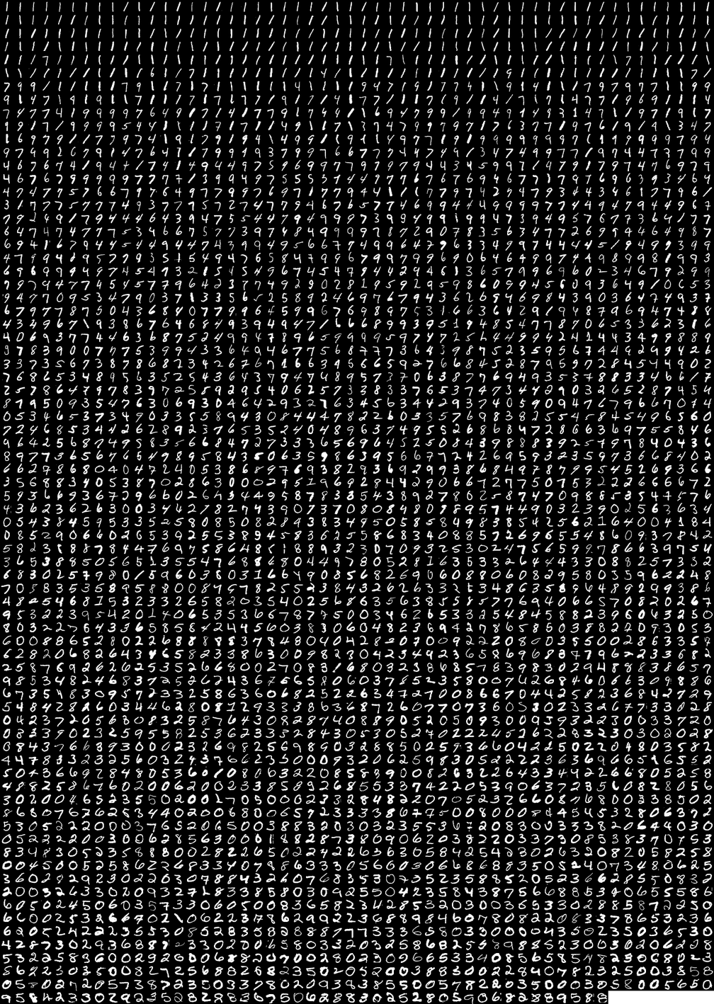
Figure 13: MNIST sorted (left to right and top to bottom) by FLIPD estimate (MLP) at $t_{0}=0.1$.

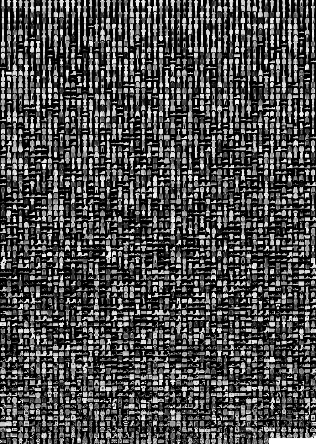
Figure 14: FMNIST sorted (left to right and top to bottom) by FLIPD estimate (MLP) at $t_{0}=0.1$.

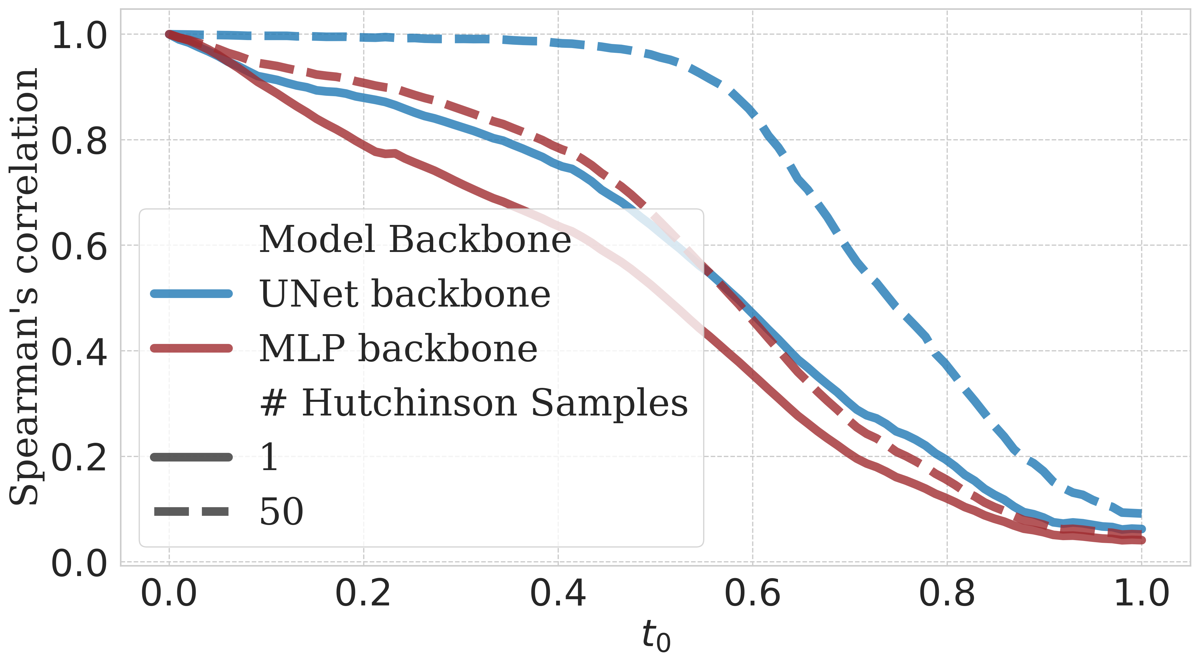
(a) Multiscale Spearman’s correlation on CIFAR10.

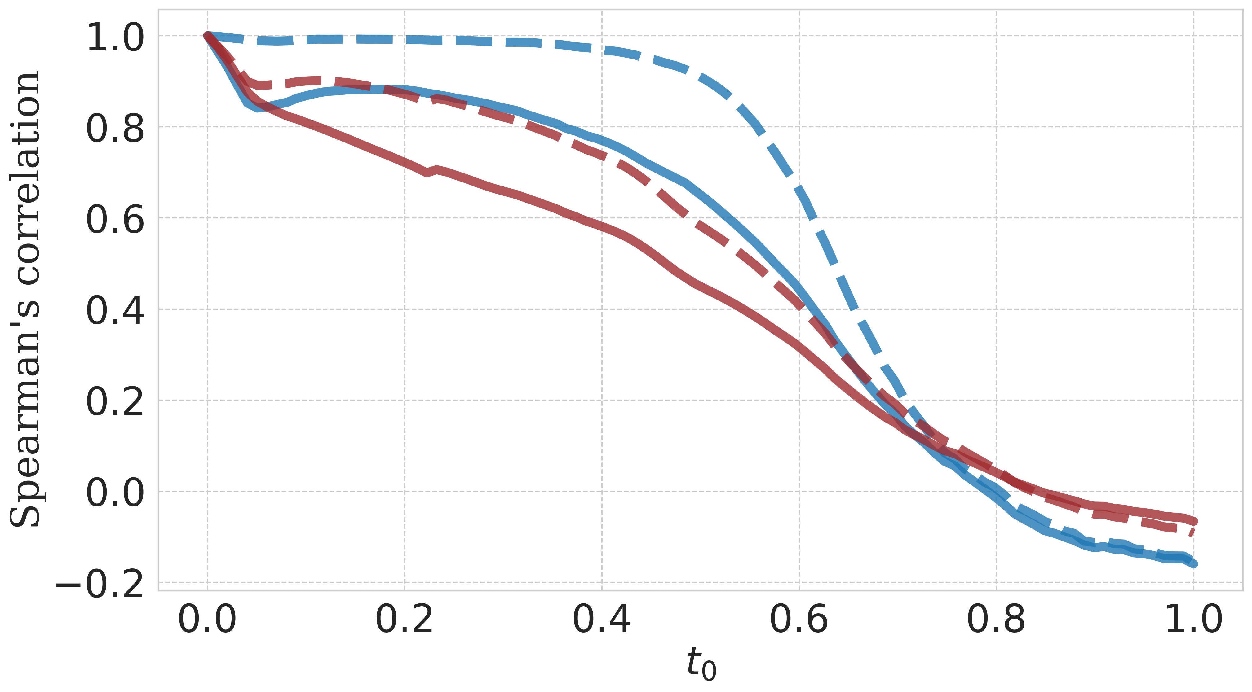
(b) Multiscale Spearman’s correlation on SVHN.

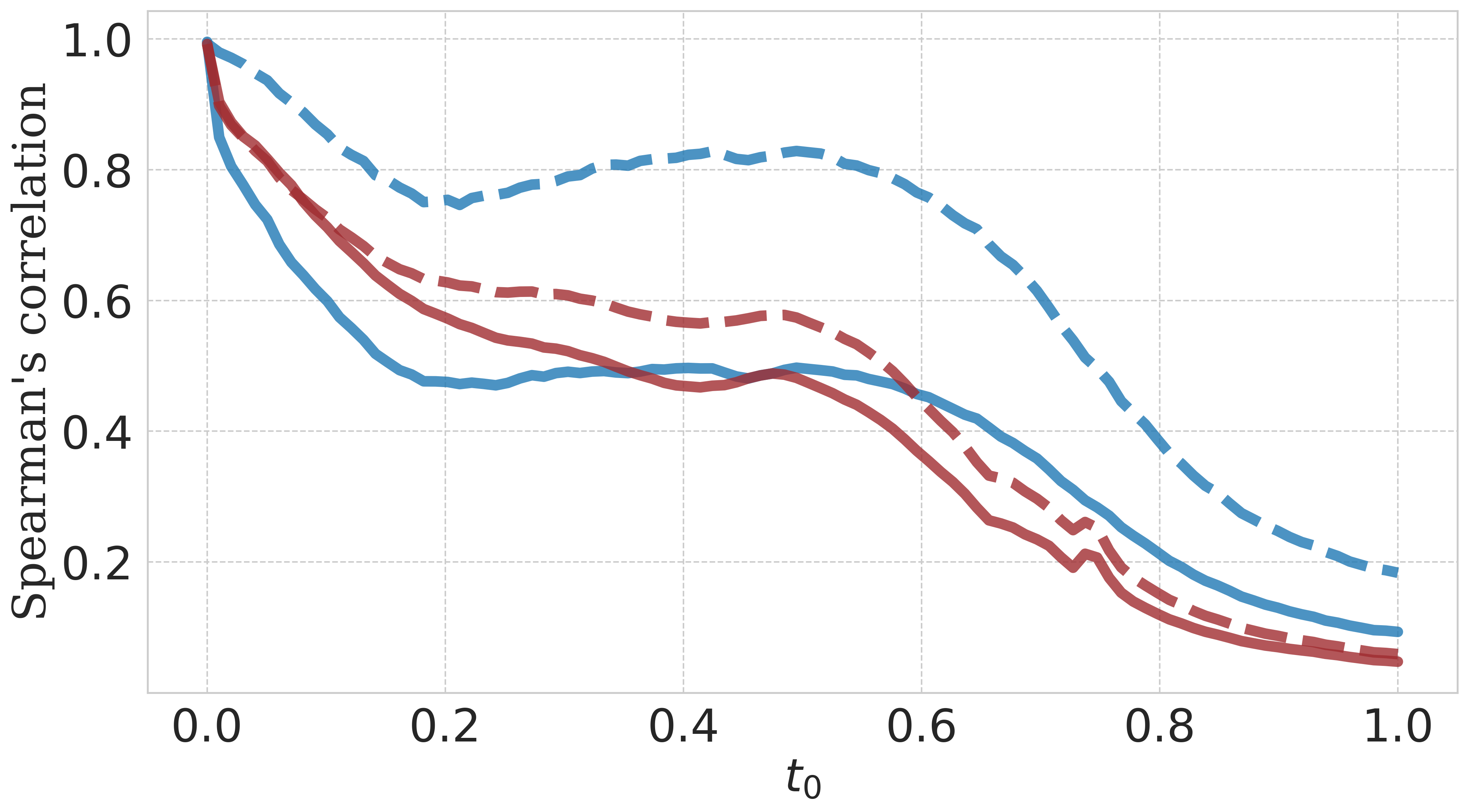
(c) Multiscale Spearman’s correlation on MNIST.

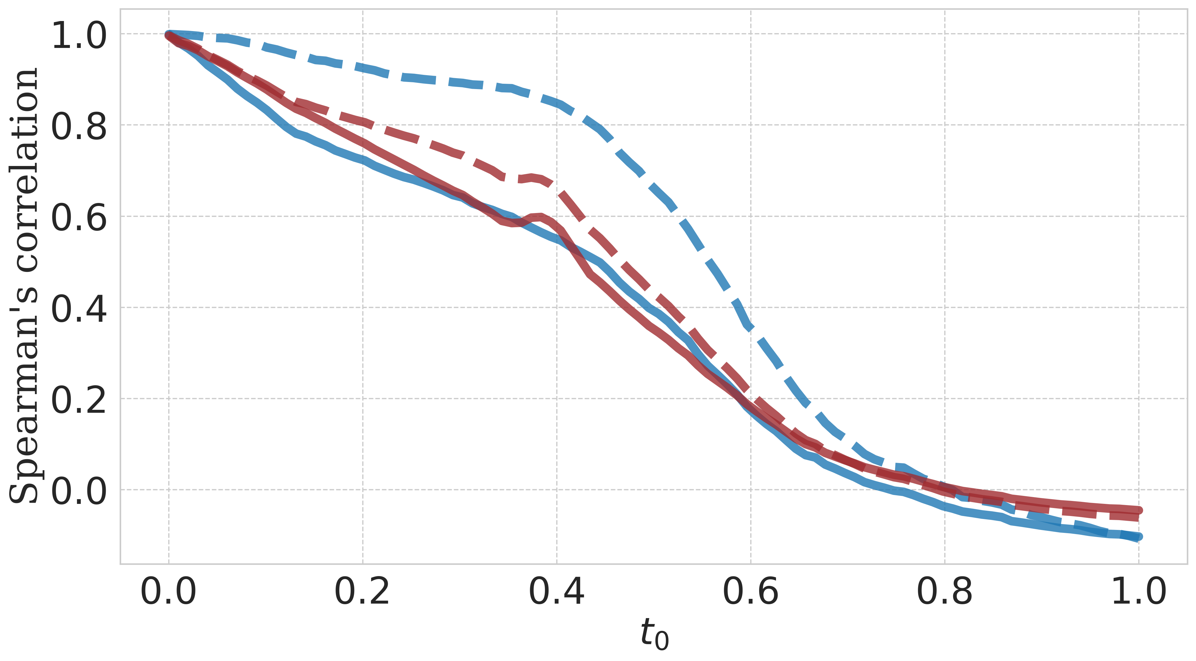
(d) Multiscale Spearman’s correlation on FMNIST.

Figure 15: Spearman’s correlation of FLIPD estimates while using different numbers of Hutchinson samples compared to computing the trace term of FLIPD deterministically with $D$ Jacobian vector product calls. These estimates are evaluated at different values of $t_{0}\in(0,1)$ on four datasets using the UNet and MLP backbones.

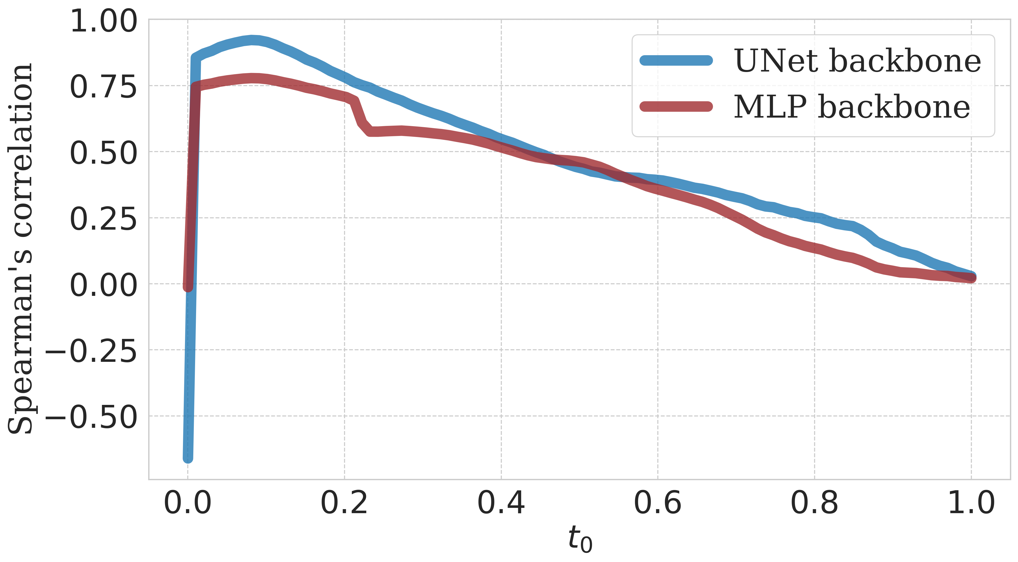
(a) Multiscale correlation with PNG on CIFAR10.

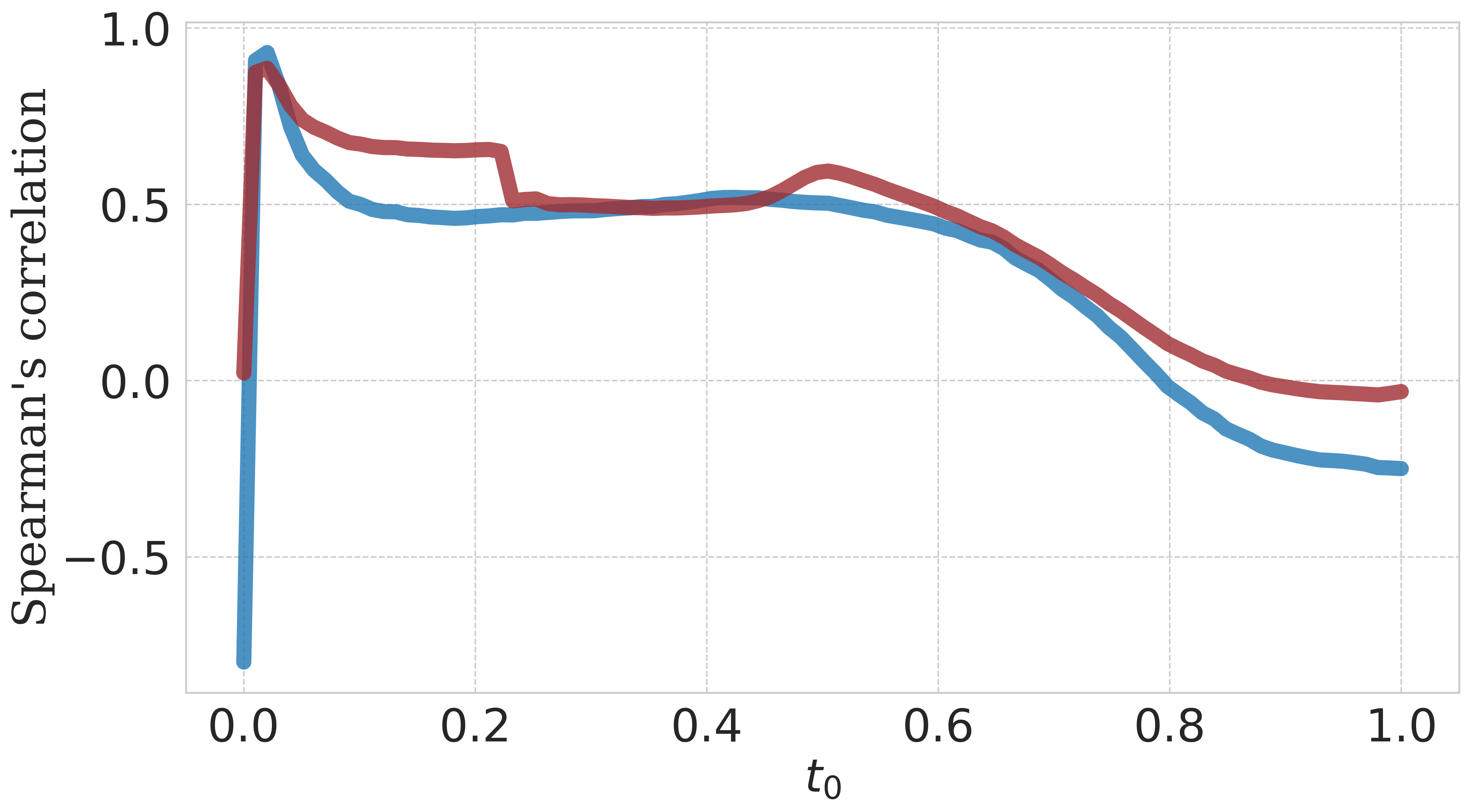
(b) Multiscale correlation with PNG on SVHN.

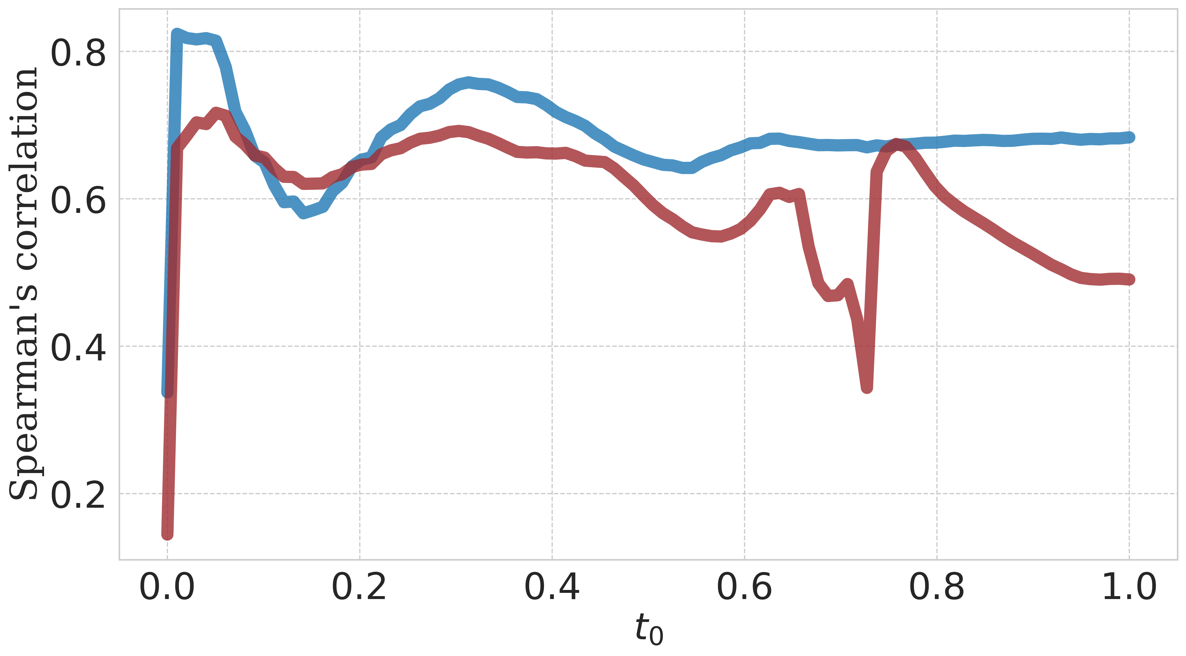
(c) Multiscale correlation with PNG on MNIST.

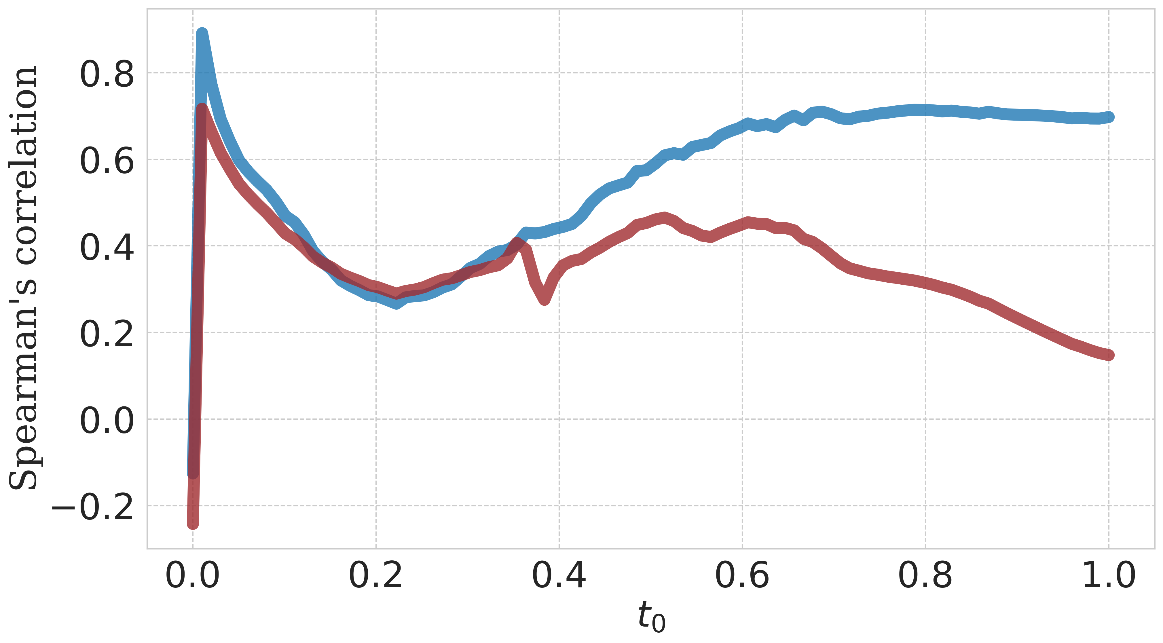
(d) Multiscale correlation with PNG on FMNIST.

Figure 16: Spearman’s correlation of FLIPD estimates with PNG as we sweep $t_{0}\in(0,1)$ on different backbones and different image datasets.

(a) $t_{0}=0.01$.

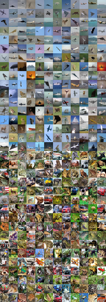
(b) $t_{0}=0.1$.

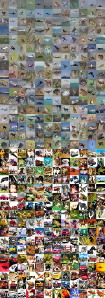
(c) $t_{0}=0.3$.

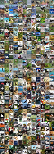
(d) $t_{0}=0.8$.

Figure 17: The 204 smallest (top) and 204 largest (bottom) CIFAR10 FLIPD estimates with UNet evaluated at different $t_{0}$.

(a) $t_{0}=0.01$.

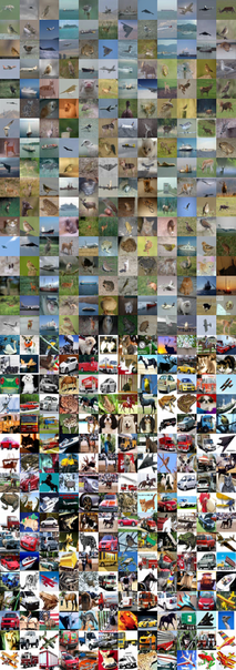
(b) $t_{0}=0.1$.

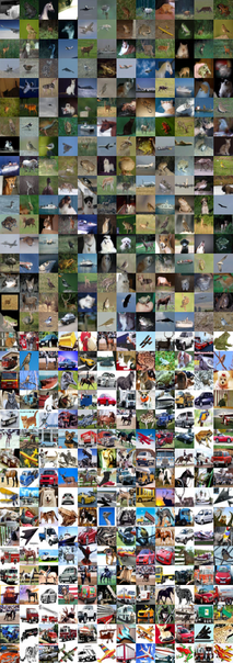
(c) $t_{0}=0.3$.

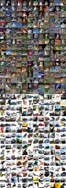
(d) $t_{0}=0.8$.

Figure 18: The 204 smallest (top) and 204 largest (bottom) CIFAR10 FLIPD estimates with MLP evaluated at different $t_{0}$.

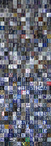
(a) $t_{0}=0.01$.

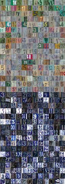
(b) $t_{0}=0.1$.

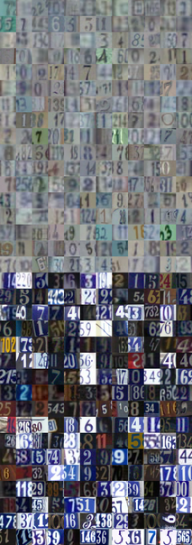
(c) $t_{0}=0.3$.

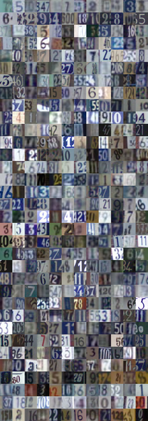
(d) $t_{0}=0.8$.

Figure 19: The 204 smallest (top) and 204 largest (bottom) SVHN FLIPD with UNet estimates evaluated at different $t_{0}$.

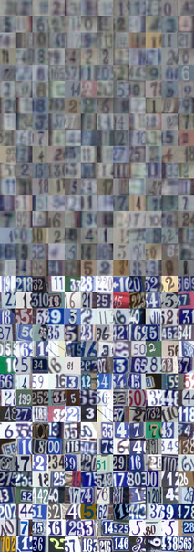
(a) $t_{0}=0.01$.

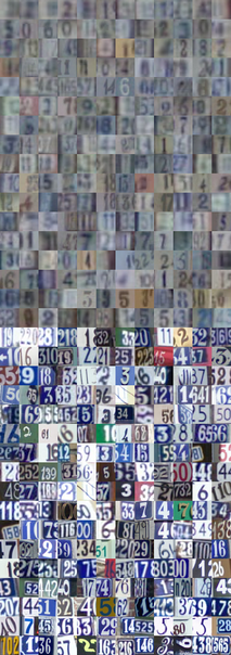
(b) $t_{0}=0.1$.

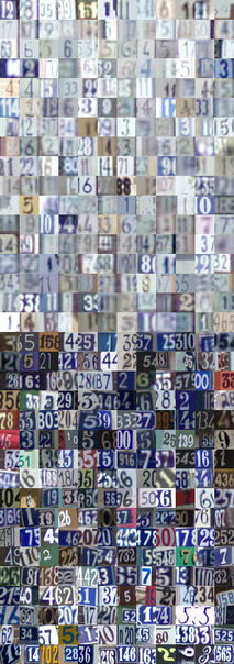
(c) $t_{0}=0.3$.

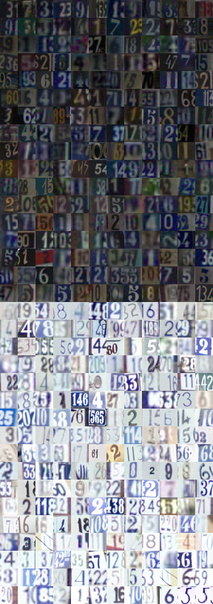
(d) $t_{0}=0.8$.

Figure 20: The 204 smallest (top) and 204 largest (bottom) SVHN FLIPD with MLP estimates evaluated at different $t_{0}$.

(a) $t_{0}=0.01$.

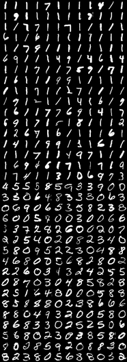
(b) $t_{0}=0.1$.

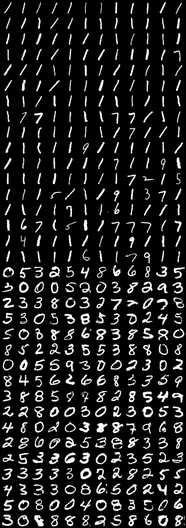
(c) $t_{0}=0.3$.

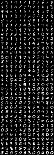
(d) $t_{0}=0.8$.

Figure 21: The 204 smallest (top) and 204 largest (bottom) MNIST FLIPD with UNet estimates evaluated at different $t_{0}$.

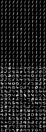
(a) $t_{0}=0.01$.

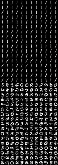
(b) $t_{0}=0.1$.

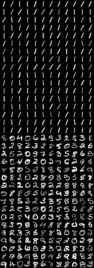
(c) $t_{0}=0.3$.

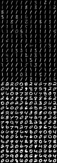
(d) $t_{0}=0.8$.

Figure 22: The 204 smallest (top) and 204 largest (bottom) MNIST FLIPD with MLP estimates evaluated at different $t_{0}$.

(a) $t_{0}=0.01$.

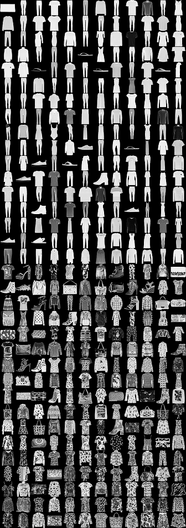
(b) $t_{0}=0.1$.

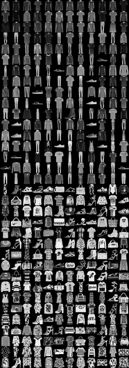
(c) $t_{0}=0.3$.

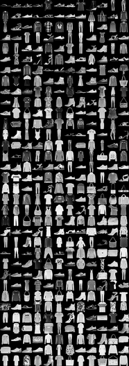
(d) $t_{0}=0.8$.

Figure 23: The 204 smallest (top) and 204 largest (bottom) FMNIST FLIPD estimates with UNet evaluated at different $t_{0}$.

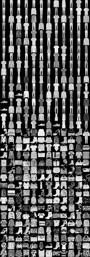
(a) $t_{0}=0.01$.

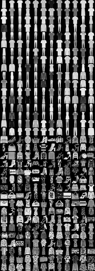
(b) $t_{0}=0.1$.

(c) $t_{0}=0.3$.

(d) $t_{0}=0.8$.

Figure 24: The 204 smallest (top) and 204 largest (bottom) FMNIST FLIPD estimates with MLP evaluated at different $t_{0}$.

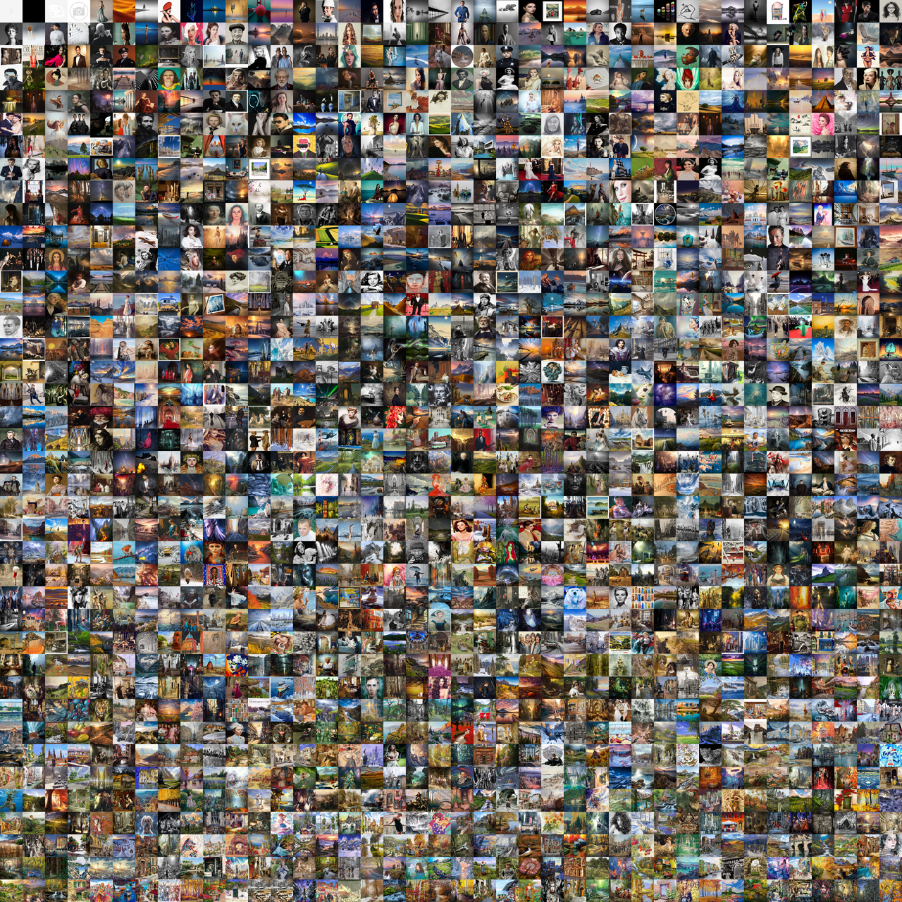
Figure 25: 1600 images from LAION-Aesthetics-625K, sorted by FLIPD estimates with $t_{0}=0.3$.

(a) $t_{0}=0.01$.

(b) $t_{0}=0.1$.

(c) $t_{0}=0.8$.

Figure 26: The 8 lowest- and highest-FLIPD values out of 1600 from LAION-Aesthetics-625k evaluated at different values of $t_{0}$. Placeholder icons or blank images have been excluded from this comparison.

References

- Albergante et al. [2019] Luca Albergante, Jonathan Bac, and Andrei Zinovyev. Estimating the effective dimension of large biological datasets using fisher separability analysis. In 2019 International Joint Conference on Neural Networks, pages 1–8. IEEE, 2019.
- Anderberg et al. [2024] Alastair Anderberg, James Bailey, Ricardo JGB Campello, Michael E Houle, Henrique O Marques, Miloš Radovanović, and Arthur Zimek. Dimensionality-aware outlier detection. In Proceedings of the 2024 SIAM International Conference on Data Mining, pages 652–660, 2024.
- Anderson [1982] Brian DO Anderson. Reverse-time diffusion equation models. Stochastic Processes and their Applications, 12(3):313–326, 1982.
- Ansuini et al. [2019] Alessio Ansuini, Alessandro Laio, Jakob H Macke, and Davide Zoccolan. Intrinsic dimension of data representations in deep neural networks. In Advances in Neural Information Processing Systems, 2019.
- Bac et al. [2021] Jonathan Bac, Evgeny M. Mirkes, Alexander N. Gorban, Ivan Tyukin, and Andrei Zinovyev. Scikit-Dimension: A Python Package for Intrinsic Dimension Estimation. Entropy, 23(10):1368, 2021.
- Baydin et al. [2018] Atılım Günes Baydin, Barak A Pearlmutter, Alexey Andreyevich Radul, and Jeffrey Mark Siskind. Automatic Differentiation in Machine Learning: A Survey. Journal of Machine Learning Research, 18:1–43, 2018.
- Bengio et al. [2013] Yoshua Bengio, Aaron Courville, and Pascal Vincent. Representation learning: A review and new perspectives. IEEE Transactions on Pattern Analysis and Machine Intelligence, 35(8):1798–1828, 2013.
- Birdal et al. [2021] Tolga Birdal, Aaron Lou, Leonidas J Guibas, and Umut Simsekli. Intrinsic dimension, persistent homology and generalization in neural networks. In Advances in Neural Information Processing Systems, 2021.
- Brown et al. [2022] Bradley CA Brown, Jordan Juravsky, Anthony L Caterini, and Gabriel Loaiza-Ganem. Relating regularization and generalization through the intrinsic dimension of activations. arXiv:2211.13239, 2022.
- Brown et al. [2023] Bradley CA Brown, Anthony L Caterini, Brendan Leigh Ross, Jesse C Cresswell, and Gabriel Loaiza-Ganem. Verifying the union of manifolds hypothesis for image data. In International Conference on Learning Representations, 2023.
- Cangelosi and Goriely [2007] Richard Cangelosi and Alain Goriely. Component retention in principal component analysis with application to cdna microarray data. Biology Direct, 2:1–21, 2007.
- Chen et al. [2018] Ricky TQ Chen, Yulia Rubanova, Jesse Bettencourt, and David K Duvenaud. Neural ordinary differential equations. In Advances in Neural Information Processing Systems, 2018.
- Cornish et al. [2020] Rob Cornish, Anthony L. Caterini, George Deligiannidis, and Arnaud Doucet. Relaxing bijectivity constraints with continuously indexed normalising flows. In International Conference on Machine Learning, pages 2133–2143, 2020.
- Cresswell et al. [2022] Jesse C Cresswell, Brendan Leigh Ross, Gabriel Loaiza-Ganem, Humberto Reyes-Gonzalez, Marco Letizia, and Anthony L Caterini. CaloMan: Fast generation of calorimeter showers with density estimation on learned manifolds. arXiv:2211.15380, 2022.
- De Bortoli [2022] Valentin De Bortoli. Convergence of denoising diffusion models under the manifold hypothesis. Transactions on Machine Learning Research, 2022.
- Dinh et al. [2017] Laurent Dinh, Jascha Sohl-Dickstein, and Samy Bengio. Density estimation using Real NVP. In International Conference on Learning Representations, 2017.
- Durkan et al. [2019] Conor Durkan, Artur Bekasov, Iain Murray, and George Papamakarios. Neural spline flows. In Advances in Neural Information Processing Systems, 2019.
- Durkan et al. [2020] Conor Durkan, Artur Bekasov, Iain Murray, and George Papamakarios. nflows: normalizing flows in PyTorch, November 2020. URL https://doi.org/10.5281/zenodo.4296287.
- Facco et al. [2017] Elena Facco, Maria d’Errico, Alex Rodriguez, and Alessandro Laio. Estimating the intrinsic dimension of datasets by a minimal neighborhood information. Scientific Reports, 7(1):12140, 2017.
- Falconer [2007] Kenneth Falconer. Fractal Geometry: Mathematical Foundations and Applications. John Wiley & Sons, 2007.
- Fukunaga and Olsen [1971] Keinosuke Fukunaga and David R Olsen. An algorithm for finding intrinsic dimensionality of data. IEEE Transactions on Computers, 100(2):176–183, 1971.
- Harrell Jr et al. [1996] Frank E Harrell Jr, Kerry L Lee, and Daniel B Mark. Multivariable prognostic models: issues in developing models, evaluating assumptions and adequacy, and measuring and reducing errors. Statistics in Medicine, 15(4):361–387, 1996.
- Haussmann and Pardoux [1986] UG Haussmann and E Pardoux. Time reversal of diffusions. The Annals of Probability, 14(4):1188–1205, 1986.
- Ho et al. [2020] Jonathan Ho, Ajay Jain, and Pieter Abbeel. Denoising diffusion probabilistic models. In Advances in Neural Information Processing Systems, 2020.
- Horvat and Pfister [2024] Christian Horvat and Jean-Pascal Pfister. On gauge freedom, conservativity and intrinsic dimensionality estimation in diffusion models. In International Conference on Learning Representations, 2024.
- Houle et al. [2018] Michael E Houle, Erich Schubert, and Arthur Zimek. On the correlation between local intrinsic dimensionality and outlierness. In Similarity Search and Applications: 11th International Conference, SISAP 2018, pages 177–191. Springer, 2018.
- Hurewicz and Wallman [1948] Witold Hurewicz and Henry Wallman. Dimension Theory (PMS-4). Princeton University Press, 1948.
- Hutchinson [1989] Michael F Hutchinson. A stochastic estimator of the trace of the influence matrix for Laplacian smoothing splines. Communications in Statistics-Simulation and Computation, 18(3):1059–1076, 1989.
- Johnsson et al. [2014] Kerstin Johnsson, Charlotte Soneson, and Magnus Fontes. Low bias local intrinsic dimension estimation from expected simplex skewness. IEEE Transactions on Pattern Analysis and Machine Intelligence, 37(1):196–202, 2014.
- Kamkari et al. [2024a] Hamidreza Kamkari, Vahid Balazadeh, Vahid Zehtab, and Rahul G. Krishnan. Order-based structure learning with normalizing flows. arXiv:2308.07480, 2024a.
- Kamkari et al. [2024b] Hamidreza Kamkari, Brendan Leigh Ross, Jesse C Cresswell, Anthony L Caterini, Rahul G Krishnan, and Gabriel Loaiza-Ganem. A geometric explanation of the likelihood OOD detection paradox. arXiv:2403.18910, 2024b.
- Kingma and Welling [2014] Diederik P Kingma and Max Welling. Auto-encoding variational Bayes. In International Conference on Learning Representations, 2014.
- Kirichenko et al. [2020] Polina Kirichenko, Pavel Izmailov, and Andrew G Wilson. Why normalizing flows fail to detect out-of-distribution data. In Advances in Neural Information Processing Systems, 2020.
- Krizhevsky and Hinton [2009] Alex Krizhevsky and Geoffrey Hinton. Learning multiple layers of features from tiny images. Technical Report, 2009.
- LeCun et al. [1998] Yann LeCun, Léon Bottou, Yoshua Bengio, and Patrick Haffner. Gradient-based learning applied to document recognition. Proceedings of the IEEE, 86(11):2278–2324, 1998.
- Lee [2012] John M Lee. Introduction to Smooth Manifolds. Springer, 2nd edition, 2012.
- Levina and Bickel [2004] Elizaveta Levina and Peter Bickel. Maximum likelihood estimation of intrinsic dimension. In Advances in Neural Information Processing Systems, 2004.
- Loaiza-Ganem et al. [2022] Gabriel Loaiza-Ganem, Brendan Leigh Ross, Jesse C Cresswell, and Anthony L. Caterini. Diagnosing and fixing manifold overfitting in deep generative models. Transactions on Machine Learning Research, 2022.
- Loaiza-Ganem et al. [2024] Gabriel Loaiza-Ganem, Brendan Leigh Ross, Rasa Hosseinzadeh, Anthony L Caterini, and Jesse C Cresswell. Deep generative models through the lens of the manifold hypothesis: A survey and new connections. arXiv:2404.02954, 2024.
- Lu et al. [2023] Yubin Lu, Zhongjian Wang, and Guillaume Bal. Mathematical analysis of singularities in the diffusion model under the submanifold assumption. arXiv:2301.07882, 2023.
- Ma et al. [2018] Xingjun Ma, Bo Li, Yisen Wang, Sarah M Erfani, Sudanthi Wijewickrema, Grant Schoenebeck, Dawn Song, Michael E Houle, and James Bailey. Characterizing adversarial subspaces using local intrinsic dimensionality. In International Conference on Learning Representations, 2018.
- MacKay and Ghahramani [2005] David JC MacKay and Zoubin Ghahramani. Comments on “Maximum likelihood estimation of intrinsic dimension’ by E. Levina and P. Bickel (2004). The Inference Group Website, Cavendish Laboratory, Cambridge University, 2005.
- Magai and Ayzenberg [2022] German Magai and Anton Ayzenberg. Topology and geometry of data manifold in deep learning. arXiv:2204.08624, 2022.
- Mayr and Petras [2008] Philipp Mayr and Vivien Petras. Cross-concordances: terminology mapping and its effectiveness for information retrieval. arXiv:0806.3765, 2008.
- Netzer et al. [2011] Yuval Netzer, Tao Wang, Adam Coates, Alessandro Bissacco, Bo Wu, and Andrew Y Ng. Reading digits in natural images with unsupervised feature learning. In NIPS Workshop on Deep Learning and Unsupervised Feature Learning, 2011.
- Pidstrigach [2022] Jakiw Pidstrigach. Score-based generative models detect manifolds. In Advances in Neural Information Processing Systems, 2022.
- Pope et al. [2021] Phil Pope, Chen Zhu, Ahmed Abdelkader, Micah Goldblum, and Tom Goldstein. The intrinsic dimension of images and its impact on learning. In International Conference on Learning Representations, 2021.
- Rezende and Mohamed [2015] Danilo Rezende and Shakir Mohamed. Variational Inference with Normalizing Flows. In Proceedings of the 32nd International Conference on Machine Learning, volume 37, pages 1530–1538, 2015.
- Rombach et al. [2022] Robin Rombach, Andreas Blattmann, Dominik Lorenz, Patrick Esser, and Björn Ommer. High-resolution image synthesis with latent diffusion models. In Proceedings of the IEEE/CVF Conference on Computer Vision and Pattern Recognition, pages 10684–10695, 2022.
- Ronneberger et al. [2015] Olaf Ronneberger, Philipp Fischer, and Thomas Brox. U-net: Convolutional networks for biomedical image segmentation. In Medical image computing and computer-assisted intervention–MICCAI 2015: 18th international conference, Munich, Germany, October 5-9, 2015, proceedings, part III 18, pages 234–241. Springer, 2015.
- Särkkä and Solin [2019] Simo Särkkä and Arno Solin. Applied stochastic differential equations. Cambridge University Press, 2019.
- Satopaa et al. [2011] Ville Satopaa, Jeannie Albrecht, David Irwin, and Barath Raghavan. Finding a "kneedle" in a Haystack: Detecting Knee Points in System Behavior. In 31st International Conference on Distributed Computing Systems Workshops, pages 166–171. IEEE, 2011.
- Schuhmann et al. [2022] Christoph Schuhmann, Romain Beaumont, Richard Vencu, Cade Gordon, Ross Wightman, Mehdi Cherti, Theo Coombes, Aarush Katta, Clayton Mullis, Mitchell Wortsman, et al. Laion-5b: An open large-scale dataset for training next generation image-text models. Advances in Neural Information Processing Systems, 35:25278–25294, 2022.
- Sohl-Dickstein et al. [2015] Jascha Sohl-Dickstein, Eric Weiss, Niru Maheswaranathan, and Surya Ganguli. Deep unsupervised learning using nonequilibrium thermodynamics. In International Conference on Machine Learning, pages 2256–2265, 2015.
- Song et al. [2021a] Yang Song, Conor Durkan, Iain Murray, and Stefano Ermon. Maximum likelihood training of score-based diffusion models. In Advances in Neural Information Processing Systems, 2021a.
- Song et al. [2021b] Yang Song, Jascha Sohl-Dickstein, Diederik P Kingma, Abhishek Kumar, Stefano Ermon, and Ben Poole. Score-based generative modeling through stochastic differential equations. In International Conference on Learning Representations, 2021b.
- Stanczuk et al. [2022] Jan Stanczuk, Georgios Batzolis, Teo Deveney, and Carola-Bibiane Schönlieb. Your diffusion model secretly knows the dimension of the data manifold. arXiv:2212.12611, 2022.
- Steck et al. [2007] Harald Steck, Balaji Krishnapuram, Cary Dehing-Oberije, Philippe Lambin, and Vikas C Raykar. On ranking in survival analysis: Bounds on the concordance index. In Advances in Neural Information Processing Systems, volume 20, 2007.
- Teles [2012] Júlia Teles. Concordance coefficients to measure the agreement among several sets of ranks. Journal of Applied Statistics, 39(8):1749–1764, 2012.
- Tempczyk et al. [2022] Piotr Tempczyk, Rafał Michaluk, Lukasz Garncarek, Przemysław Spurek, Jacek Tabor, and Adam Golinski. LIDL: Local intrinsic dimension estimation using approximate likelihood. In International Conference on Machine Learning, pages 21205–21231, 2022.
- Tulchinskii et al. [2023] Eduard Tulchinskii, Kristian Kuznetsov, Laida Kushnareva, Daniil Cherniavskii, Sergey Nikolenko, Evgeny Burnaev, Serguei Barannikov, and Irina Piontkovskaya. Intrinsic dimension estimation for robust detection of ai-generated texts. In Advances in Neural Information Processing Systems, 2023.
- Vahdat et al. [2021] Arash Vahdat, Karsten Kreis, and Jan Kautz. Score-based generative modeling in latent space. In Advances in Neural Information Processing Systems, 2021.
- Valeriani et al. [2023] Lucrezia Valeriani, Diego Doimo, Francesca Cuturello, Alessandro Laio, Alessio Ansuini, and Alberto Cazzaniga. The geometry of hidden representations of large transformer models. In Advances in Neural Information Processing Systems, 2023.
- Vincent [2011] Pascal Vincent. A connection between score matching and denoising autoencoders. Neural Computation, 23(7):1661–1674, 2011.
- von Platen et al. [2022] Patrick von Platen, Suraj Patil, Anton Lozhkov, Pedro Cuenca, Nathan Lambert, Kashif Rasul, Mishig Davaadorj, and Thomas Wolf. Diffusers: State-of-the-art diffusion models. https://github.com/huggingface/diffusers, 2022.
- Xiao et al. [2017] Han Xiao, Kashif Rasul, and Roland Vollgraf. Fashion-MNIST: A novel image dataset for benchmarking machine learning algorithms. arXiv:1708.07747, 2017.
- Xue et al. [2022] Fanghui Xue, Biao Yang, Yingyong Qi, and Jack Xin. Searching intrinsic dimensions of vision transformers. arXiv:2204.07722, 2022.
- Zheng et al. [2022] Yijia Zheng, Tong He, Yixuan Qiu, and David P Wipf. Learning manifold dimensions with conditional variational autoencoders. In Advances in Neural Information Processing Systems, 2022.
- Zhu et al. [2018] Wei Zhu, Qiang Qiu, Jiaji Huang, Robert Calderbank, Guillermo Sapiro, and Ingrid Daubechies. Ldmnet: Low dimensional manifold regularized neural networks. In Proceedings of the IEEE Conference on Computer Vision and Pattern Recognition, pages 2743–2751, 2018.