Precise interpretations of traditional fine-tuning measures
Abstract
We uncover two precise interpretations of traditional electroweak fine-tuning (FT) measures that were historically missed. (i) a statistical interpretation: the traditional FT measure shows the change in plausibility of a model in which a parameter was exchanged for the boson mass relative to an untuned model in light of the boson mass measurement. (ii) an information-theoretic interpretation: the traditional FT measure shows the exponential of the extra information, measured in nats, relative to an untuned model that you must supply about a parameter in order to fit the mass. We derive the mathematical results underlying these interpretations, and explain them using examples from weak scale supersymmetry. These new interpretations shed fresh light on historical and recent studies using traditional FT measures.
I Introduction
Although the concepts of fine-tuning and naturalness are under pressure [Richter:2006um, Dine:2015xga, Hossenfelder:2018ikr], they remain popular among physicists [tHooft:1979rat, ef2165c8-7176-35d7-a191-db6afd794cac, Feng:2013pwa, Giudice:2008bi, Craig:2022eqo, Wells:2018yyb]. Efforts to define and measure fine-tuning began in the context of supersymmetric models in the 1980s. Ref. [Ellis:1986yg, Barbieri:1987fn] introduced a measure of fine-tuning of the parameter to fit the mass,
| (1) |
We refer to this as the traditional fine-tuning (FT) measure.111Equation 1 may be more commonly known as the Barbieri-Giudice measure or as the Barbieri-Giudice-Ellis-Nanopoulos measure. The traditional FT measure shows sensitivity in the parameter . To aggregate traditional FT measures for more than one parameter, ref. [Ellis:1986yg, Barbieri:1987fn] suggested maximizing across them,
| (2) |
There are, however, other possibilities, e.g., adding traditional FT measures in quadrature [Casas:2004gh]. By these measures, fine tuning in supersymmetric models became severe after results from LEP [Anderson:1994tr, Chankowski:1997zh, Barbieri:1998uv, Chankowski:1998xv, Kane:1998im] and even worse after results from LHC runs I and II [Strumia:2011dv, Baer:2012mv, Arvanitaki:2013yja, Baer:2014ica, vanBeekveld:2019tqp]. The severity of fine tuning led to doubts about weak scale supersymmetry; however, the measure of fine tuning appears somewhat arbitrary and lacking in precise meaning. Efforts to connect fine tuning with a probability of cancellations [Anderson:1994dz, Ciafaloni:1996zh, Giusti:1998gz, Strumia:1999fr, Allanach:2006jc, Athron:2007ry] ultimately led to an interpretation of fine tuning in Bayesian inference [Allanach:2007qk, Cabrera:2008tj, Cabrera:2010dh, Balazs:2012vjy, Fichet:2012sn, Fowlie:2014faa, Fowlie:2014xha, Fowlie:2015uga, Clarke:2016jzm, Fowlie:2016jlx, Athron:2017fxj, Fundira:2017vip]. Indeed, traditional FT measures were shown to appear as factors in integrands in intermediate stages of Bayesian inference. A precise interpretation of the measures themselves, however, remained lacking (see appendix B for further discussion).
We recently proposed the Bayes factor (BF) surface [Fowlie:2024dgj] as a new way to understand the impact of experimental measurements on models of new physics.222See ref. [gram2020, Johnson_2023, Wagenmakers2020, Pawel2023, NANOGrav:2023hvm] for recent related works in other contexts. Considering the measurement of the mass, the BF surface reveals a precise statistical interpretation of traditional fine-tuning measures. In particular, we will demonstrate that fine-tuning maps are exactly equivalent to a BF surface.
We have, furthermore, discussed in recent years applications of information theory in interpreting experimental searches of new physics, e.g., ref. [Fowlie:2017ufs, Fowlie:2018svr, Herrera:2024zrk]. Interestingly, we will demonstrate here that the Kullback-Leibler divergence [Kullback:1951zyt] is connected to the BF surface and traditional FT measures. Concretely, traditional FT measures show exactly the exponential of the extra information, measured in nats, required to predict the mass.
II Interpreting mass measurement
II.1 Bayes factor surface
The Bayes factor (BF) surface [Fowlie:2024dgj] shows the change in plausibility of a model as a function of that model’s parameters relative to a reference model. For the evidence in favor of the reference model, we may write this as
| (3) |
where and are the evidences for the model and reference model, respectively. The evidences themselves are likelihoods averaged over a choice of prior [Jeffreys:1939xee, kass1995bayes];
| (4) |
for likelihood and prior .
First, consider a trivial toy model with a single parameter , that predicts the mass as
| (5) |
We refer to this as an untuned model. The narrow Gaussian for the combined mass measurement, [Workman:2022ynf], may be approximated by a Dirac function,
| (6) |
Thus the evidence for this untuned model may be written,
| (7) |
where such that .
Second, consider a complicated model with parameters that predicts the mass as
| (8) |
This model could be, for example, weak-scale supersymmetry. To predict the correct mass, we assume that the parameter was exchanged for the mass. We denote the remaining parameters by . For this complicated model,
| (9) |
where is a function of such that .
We now consider the BF between the untuned and complicated model as a function of — this is the BF surface. Using eqs. 7 and 9, we find
| (10) |
Our notation indicates that the parameter was marginalized. Equation 10 depends on choices of prior for the model parameters. The scale-invariant density, , weights every order of magnitude equally [4082152, Hartigan1964, Consonni2018]. Consider an identical scale-invariant prior for in the untuned and complicated model,
| (11) |
over the range to . With this choice, we obtain,
| (12) |
where the dependence on and canceled.
II.2 Information
The Kullback-Leibler (KL) divergence [Kullback:1951zyt] between the prior and the posterior for a model parameter may be written as,
| (13) |
The KL divergence can be interpreted as a measure of information learned about from the measurement of the mass or compression from the prior to the posterior [mackay2003information]. Consider, for example, a one-dimensional model with a unit uniform prior for parameter . Suppose that we measured . We would find that — we learned of information about and compressed by .333With a natural logarithm in the KL divergence, as in eq. 13, information is measured in nats; with a base 2 logarithm, it is measured in bits. They are connected by .
Using eq. 13 and recognizing that by Bayes’ theorem, , we may express the evidence as [Hergt:2021qlh],
| (14) |
where indicates a posterior mean. Expressing eq. 14 in words reveals a Bayesian form of Occam’s razor [Hergt:2021qlh, Rosenkrantz1977, 37c684a3-9d55-37ab-ba95-6e4da1d0a51b, 1991BAAS...23.1259J, Henderson_Goodman_Tenenbaum_Woodward_2010, 4018651d-dd41-3908-8c4f-09d2118c5612, 10.1093/oxfordhb/9780199957996.013.14, mackay2003information, Blanchard2017, McFadden2023],
| (15) |
as models are penalized for fine tuning measured by the KL divergence. From eq. 14, furthermore, the Bayes factor may be written,444To avoid ambiguity, we denote differences by and the traditional FT measure by .
| (16) |
For the measurement of the mass, we find that
| (17) |
This happens because, regardless of the model, a posteriori it must predict that because of the Dirac function in eq. 6. This means that the goodness-of-fit contributions to the Bayes factor in eq. 16 cancel.
III Interpreting fine tuning
| Jeffreys [Jeffreys:1939xee] | Lee & Wagenmakers [lee2014bayesian] | Kass & Raftery [kass1995bayes] | |||
|---|---|---|---|---|---|
| to | Barely worth mentioning | 1 to 3 | Anecdotal | 1 to 3 | Barely worth mentioning |
| to | Substantial | 3 to 10 | Moderate | 3 to 20 | Positive |
| to | Strong | 10 to 30 | Strong | 20 to 150 | Strong |
| to | Very strong | 30 to 100 | Very strong | Very strong | |
| Decisive | Extreme | ||||
III.1 Equivalence
Using eqs. 12, 16 and 1, we thus find
| (18) |
or in words, using the parameter to fix the mass,
| (19) |
relative to an untuned model that predicts . This required us to choose identical scale-invariant priors for the parameters exchanged for the mass and approximate the narrow Gaussian measurement of the mass by a Dirac function, though see appendix A where we justify these requirements. In particular, in App. A.2 we checked the Dirac function approximation to a Gaussian likelihood. We found that corrections depended only on second-order variations of the prior prediction for the mass around the peak of the Gaussian measurement.
III.2 Interpretation
Equation 18 provides two precise interpretations of the traditional FT measure,
-
•
Statistical — the traditional FT measure shows the Bayes factor surface versus an untuned model. That is, it measures the change in plausibility of a model relative to an untuned model in light of the mass measurement.
-
•
Information-theoretic — the traditional FT measure shows the compression versus an untuned model. That is, it measures the exponential of the extra information, measured in nats, relative to an untuned model that you must supply about a parameter in order to fit the mass.555Similarly, ref. [Dermisek:2016zvl] proposed counting the number of digits to which a parameter must be specified to predict the correct mass.
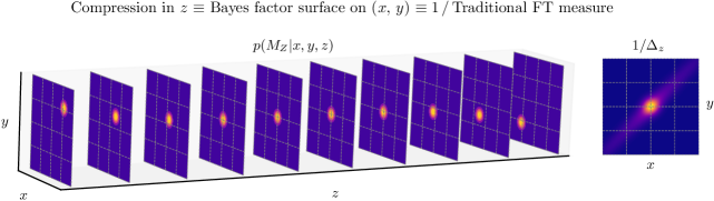
For illustration, in fig. 1 we show these interpretations in a three-dimensional toy model. The tuning and compression required in the -direction changes across the (, ) plane. The traditional FT measure on the (, ) plane shows the required compression.
Bayes factors themselves may be interpreted by ascribing qualitative meanings to them. Table 1 shows scales for interpreting a Bayes factor [Jeffreys:1939xee, lee2014bayesian, kass1995bayes]. Jeffreys [Jeffreys:1939xee] and Lee & Wagenmakers [lee2014bayesian] take and , respectively, as a threshold for very strong evidence, and as a threshold of moderate evidences. The thresholds and were chosen as thresholds for fine-tuning measures in ref. [Barbieri:1987fn] and [Baer:2015rja], respectively.
Lastly, traditional FT measures are frequently reported as a percentage tuning, , such that, e.g., represents a tuning. In fact, the percentage tuning approximately equals the posterior probability of the complicated model,
| (20) |
where and are the prior probabilities of the untuned and complicated models, respectively. The approximation holds whenever , and the untuned and complicated models are the only models under consideration and are equally plausible a priori. In these cases, a tuning of e.g., means that the complicated model was reduced to plausibility by the mass measurement.
III.3 Choice of parameter
To apply the traditional FT measure in eq. 1, one must choose a parameter with which to take a derivative, or a way in which to combine traditional FT measures for all parameters, such as eq. 2. Similarly, in the Bayes factor surface, one parameter must be marginalized to exchange for the mass. This choice defines different Bayes factor surfaces. For example, in the context of the constrained minimal supersymmetric Standard Model (CMSSM) with parameters , , , and , we could consider the surface for , , and for marginalized, or the surface for , , and for marginalized.
On the other hand, by eq. 18, the maximum traditional FT measure may be interpreted as
-
•
Statistical — the Bayes factor against the worst model that fits the mass by exchanging one parameter.
-
•
Information-theoretic — the exponential of the maximum extra information, measured in nats, that must be specified to fit the mass by exchanging one parameter.
The Bayes factor and extra information are both relative to an untuned model.
IV Examples
We now present examples from supersymmetric models — the original context in which the traditional FT measure was proposed. We use full one-loop and leading two-loop electroweak symmetry breaking conditions and two-loop renormalization group equations.666We used the MssmSoftsusy::fineTune method from SOFTSUSY-4.1.20 [Allanach:2001kg].
IV.1 Minimal Supersymmetric Standard Model
The minimal supersymmetric Standard Model (MSSM) predicts that at tree-level [Martin:1997ns]
| (21) |
where and are soft-breaking Higgs mass parameters, is the ratio of Higgs vacuum expectation values, and is a supersymmetry-preserving Higgs mass parameter.
We take a well-tempered neutralino benchmark in the MSSM from Snowmass 2013 [Cahill-Rowley:2013gca]. In this scenario, the neutralino is a well-tempered admixture of bino-higgsino and plays the role of dark matter. The tuning for this benchmark with respect to the -parameter, , indicates that, if exchanging for the mass,
-
•
Statistical — This scenario disfavored by a factor of about 20 relative to an untuned model.
-
•
Information-theoretic — An extra of information must be supplied about the parameter to fit the mass relative to an untuned model.
The worst tuning, , was with respect to the gluino mass parameter, . If this parameter were treated as unknown and marginalized in exchange for the mass, the scenario would be disfavored by more than 1000 and more than an extra of information about would be required to fit the mass.
IV.2 Constrained MSSM
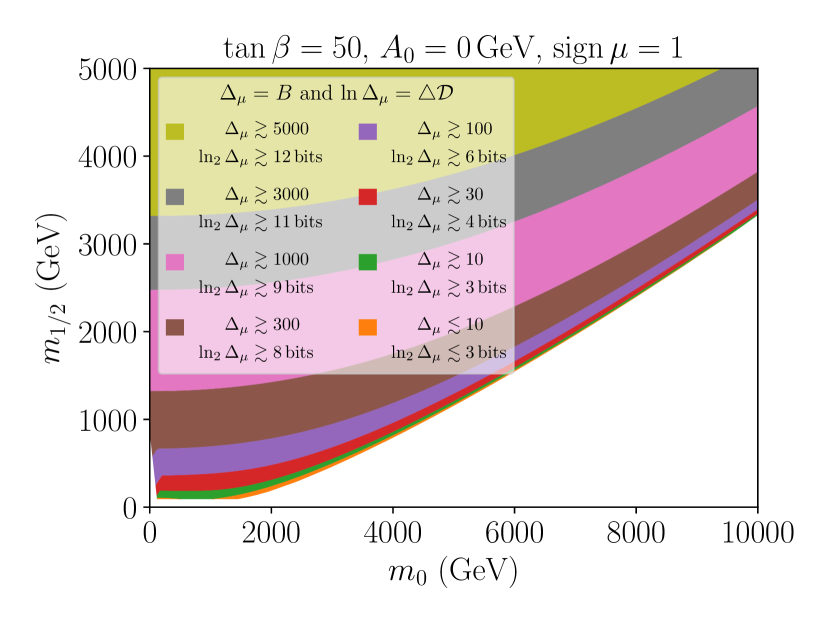
We consider the constrained MSSM (CMSSM; [Kane:1993td, Chamseddine:1982jx]). The MSSM soft-breaking terms are unified at the unification sale, leaving a universal scalar soft-breaking mass , a universal gaugino soft-breaking mass , and a universal trilinear term . In fig. 2, we show the , and slice of the (, ) plane. The traditional FT measure for the parameter, , increases from around 1 to over 5000 as increases. Besides the informal interpretation that the traditional FT measure represents undesirable and unnatural fine tuning in the parameter, there are two precise and exact interpretations:
-
•
Statistical — The traditional FT measure shows the decrease in plausibility in this model in which was unknown relative to an untuned model.
-
•
Information-theoretic — The traditional FT measures the extra information that must be supplied about the parameter to fit the mass relative to an untuned model.
For example, relative to an untuned model, models with decrease in plausibility by more than a factor 300 in light of the mass, and at least an extra of information must be supplied about the parameter to fit the mass.
Heavier gaugino masses result in fine-tuning as gaugino masses contribute radiatively to terms in eq. 21. Figure 2 shows, however, a narrow strip of parameter points fine-tuned by that extends to multi-TeV — this is the focus point region [Feng:1999zg, Feng:1999mn, Feng:2000gh, Feng:2011aa]. As we consider , eq. 21 may be approximated by
| (22) |
In the focus point region, the renormalization group equations (RGEs) focus the soft-breaking supersymmetric masses at the weak scale. That is, at the weak scale the soft-breaking Higgs mass regardless of the ultraviolet boundary condition for . This focusing means that we do not need to fine tune cancellations between and .
IV.3 Combining fine-tuning and the Higgs mass measurement
The traditional FT measure results from applying the mass measurement to a model in a Bayesian framework. This framework tells us how to combine it with other measurements. For example, we now consider the Higgs mass measurement, [Workman:2022ynf]. This Higgs mass can be realized in the CMSSM through loop corrections from heavy sparticles, at the cost of fine tuning. The statistical interpretation of the traditional FT measure sheds light on this interplay.
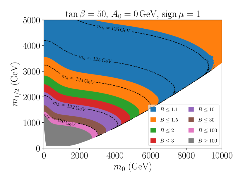
We suppose that our toy untuned model predicts that , and use a two-loop prediction from the CMSSM from SOFTSUSY-4.1.20 [Allanach:2001kg]. We assume that both predictions are known to within an uncertainty of . For illustration, we show the BF surface for the Higgs mass measurement in fig. 3. Parameters with and in the narrow focus point strip predict and are just as good as the untuned model, thus .
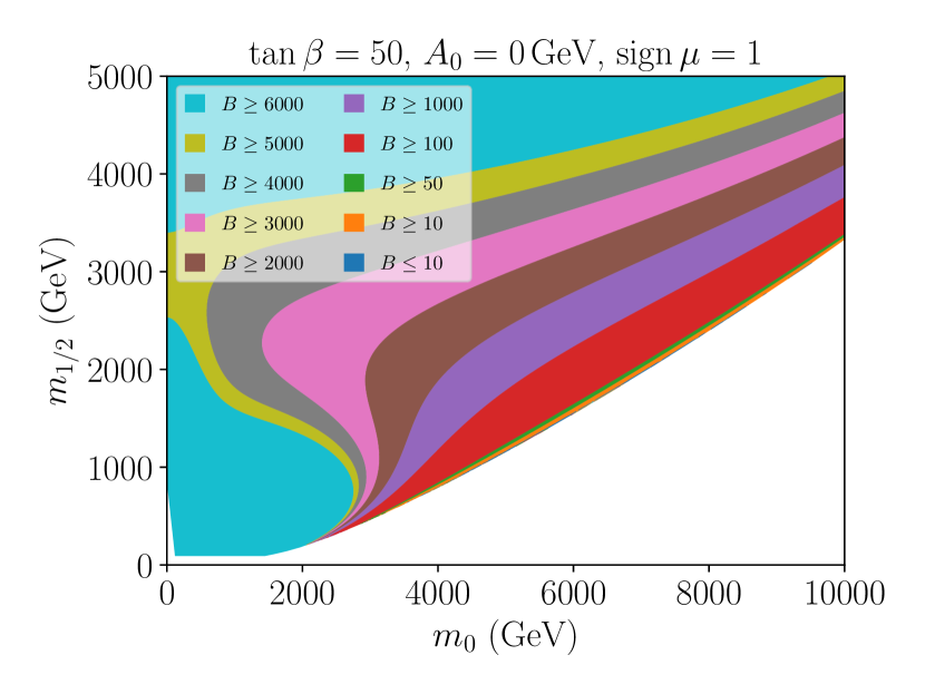
We should, however, apply the and Higgs mass measurements simultaneously. To combine them, we multiply the BF surface for the Higgs mass by the traditional FT measure for the mass,777We neglect common nuisance parameters, e.g., the mass of the top quark. If they were included, the BF surfaces could not be simply multiplied.
| (23) | ||||
| (24) | ||||
| (25) |
We retain the statistical interpretation, though lose the information-theoretic one as the BF surface for the Higgs mass contains both relative information and goodness-of-fit contributions.
We see in fig. 4 that the resulting BF surface favors the untuned model by more than , except in the focus point strip. For focus points, the untuned model could be favored by less than a factor of .
V Conclusions
Fine-tuning measures have played an important role in our assessment of theories of new physics since the 1980s. For example, doubts were raised about weak scale supersymmetric theories based on calculations of the fine-tuning prices of LEP in the 1990s, and more recently the LHC. For the first time, we provide precise interpretations of the traditional measure of fine tuning:
-
•
Statistical — the traditional FT measure shows us the change in plausibility of a model in which one parameter was exchanged for the mass relative to an untuned model in light of the mass measurement.
-
•
Information-theoretic — the traditional FT measure shows the exponential of the extra information, measured in nats, relative to an untuned model that you must supply about a parameter in order to fit the mass.
These interpretations shed fresh light on hundreds of recent and historical studies of fine tuning in supersymmetric models and models of new physics.
Lastly, these interpretations apply far beyond weak-scale supersymmetry and fine-tuning of the weak scale. They apply anywhere fine-tuning arguments were applied, e.g., cosmology, dark matter, the cosmological constant and inflation, and especially in cases of a sharp measurement that can be approximated by a Dirac function.
Acknowledgements.
Acknowledgments AF was supported by RDF-22-02-079. GH is supported by the U.S. Department of Energy under the award number DE-SC0020250 and DE-SC0020.Appendix
App. A Requirements
A.1 Scale-invariant prior
To identify the Bayes factor surface and extra information with the traditional FT measure, in eq. 11 we assumed a scale-invariant prior for the parameter exchanged for the mass. Priors are a thorny issue in Bayesian inference.
The scale-invariant prior is a common choice for unknown scales, as the density is invariant under rescaling [4082152, Hartigan1964, Consonni2018]. Because the density for the logarithm is constant,
| (26) |
it is also known as a logarithmic prior. Over the whole real line, this prior would be improper and we thus considered a proper prior by truncating it between and . This choice is not compatible with zero, e.g., , and so our interpretation of the traditional FT somewhat breaks down.
Although the scale invariant could be a reasonable choice, it is not necessarily our recommended prior. This choice of prior served to demonstrate an interpretation of the traditional FT measure: if this was our prior, we could identify the traditional FT measure with a BF surface and the extra information required to fit the mass.
A.2 Dirac approximation
In eq. 6, we approximated the likelihood function for the measurement of the mass, [Workman:2022ynf], by a Dirac function. We now consider a Gaussian likelihood, ,
| (27) |
For simplicity, we denote expectations of this Gaussian as,
| (28) |
To justify our Dirac approximation, we use techniques that are related to a Laplace approximation [doi:10.1080/01621459.1986.10478240].
Evidences
Using our notation eq. 28, we may the write evidences, e.g., eqs. 7 and 9, as,
| (29) |
where, by the Jacobian rule, the prior density of the mass,
| (30) |
In this notation, the Dirac approximation leads to
| (31) |
We now compare this to results from the Gaussian likelihood in eq. 27.
Assuming the prior varies slowly around the peak of the Gaussian likelihood, , we can perform a Taylor expansion around , such that
| (32) |
The evidence thus reads
| (33) |
Using the moments of a Gaussian distribution,
| (34a) | |||
| (34b) | |||
| (34c) | |||
| (34d) | |||
| (34e) | |||
we obtain
| (35) |
Thus, the evidence equals that in the Dirac approximation, eq. 31, up to second-order variations in the prior around .
Average goodness-of-fit
Let us now justify the Dirac approximation in the average goodness-of-fit contributions to the Bayes factor. We assumed that in eq. 16 can be neglected. First, by Bayes’ theorem the posterior for the mass may be written,
| (36) |
Second, the average goodness-of-fit can be written as an average over the predicted mass,
| (37) |
Using eq. 36 and our notation eq. 28, we write this as,
| (38) |
Through eq. 27, we express the log-likelihood appearing in eq. 38 as,
| (39) |
such that,
| (40) |
As before in eq. 32, we make a Taylor expansion for the prior such that
| (41) |
Using the moments of a Gaussian in eq. 34, we obtain
| (42) |
Thus, the average goodness-of-fit may be written,
| (43) |
Finally, the first two terms in eq. 43 cancel in differences in average of goodness-of-fit; thus,
| (44) |
That is, the difference in average goodness-of-fit depends on second-order variations of the prior prediction around .
A.3 Model priors
To identify the posterior probability of a model with , we assumed that . This assumption was only necessary for eq. 20.
App. B Previously known connections
The connections between fine-tuning and Bayesian inference were previously known and discussed in e.g. ref. [4018651d-dd41-3908-8c4f-09d2118c5612, 1991BAAS...23.1259J, mackay2003information] and explored in the specific context of weak-sale supersymmetry in ref. [Allanach:2007qk, Cabrera:2008tj, Cabrera:2010dh, Balazs:2012vjy, Fichet:2012sn, Fowlie:2014faa, Fowlie:2014xha, Fowlie:2015uga, Clarke:2016jzm, Fowlie:2016jlx, Athron:2017fxj, Fundira:2017vip]. The precise connection between traditional FT measures and Bayesian inference was hindered by the fact that the traditional FT measure cannot be directly identified with any objects in traditional Bayesian inference.
The connections required a scale-invariant prior for the -parameter. First, it was known that upon marginalizing parameters including the -parameter to produce e.g., a one-dimensional posterior density, the traditional FT measure for the -parameter would appear under integration from a combination of the scale-invariant prior and a Jacobian,
| (45) |
That is, the traditional FT measure appears as a factor in the integrand in the posterior. The posterior, however, is a density; it depends on choice of parameterization and cannot be compared to the traditional FT measure, a number. Second, it was known that the traditional FT measure appeared as factor in the integrand in the Bayesian evidence for the mass,
| (46) |
The traditional FT measure depends on choices of parameters; thus cannot be readily compared to the evidence, as they are marginalized in the latter. Thus, the connections eqs. 45 and 46 are insightful but do not allow a direct interpretation of the traditional FT measure.
App. C Minimizing fine-tuning
The traditional FT measure depends on a choice of parameters; it is common to minimize it with respect to these parameters,
| (47) |
This is a min-max equation. On the other hand, consider the Bayes factor for a model in which we marginalize every parameter according to the prior ,
| (48) |
By considering the maximum of the integrand, the Bayes factor must satisfy,
| (49) |
This must hold for every choice . Suppose that for every parameter we picked a scale-invariant prior that spanned the same number of orders of magnitude. The ratio of evidences could be written in terms of the traditional FT measure for every ,
| (50) |
As this must hold for every choice , the strongest bound becomes,
| (51) |
We thus find that minimizing fine-tuning results in a bound on the Bayes factor.
Our eq. 51, however, is a max-min inequality. For every parameter, we minimize the traditional FT measure, and finally take the maximum across choice of parameter. Max-min and min-max are connected by max-min inequalities [boyd2004convex],
| (52) |
Thus, unfortunately, we cannot chain inequalities (51) and (52). Rather than computing eq. 47, we should consider computing eq. 51, as it bounds the evidence against a model and the information that must be provided to tune the mass relative to an untuned model.
,refs.bib