Fractional Chern Insulators in Twisted Bilayer MoTe₂: A Composite Fermion Perspective

Abstract

The discovery of Fractional Chern Insulators (FCIs) in twisted bilayer MoTe₂ has sparked significant interest in fractional topological matter without external magnetic fields. Unlike the flat dispersion of Landau levels, moiré electronic states are influenced by lattice effects within a nanometer-scale superlattice. This study examines the impact of these lattice effects on the topological phases in twisted bilayer MoTe₂, uncovering a family of FCIs with Abelian anyonic quasiparticles. Using a composite fermion approach, we identify a sequence of FCIs with fractional Hall conductivities $\sigma_{xy}=\frac{C}{2C+1}\frac{e^{2}}{h}$ linked to partial filling $\nu_{\,\text{h}}$ of holes of the topmost moiré valence band. These states emerge from incompressible composite fermion bands of Chern number $C$ within a complex Hofstadter spectrum. This approach explains FCIs with Hall conductivities $\sigma_{xy}=(2/3)e^{2}/h$ and $\sigma_{xy}=(3/5)e^{2}/h$ at fractional fillings $\nu_{\,\text{h}}=2/3$ and $\nu_{\,\text{h}}=3/5$ observed in experiments, and uncovers other fractal FCI states. The Hofstadter spectrum reveals new phenomena, distinct from Landau levels, including a higher-order Van Hove singularity (HOVHS) at half-filling, leading to novel quantum phase transitions. This work offers a comprehensive framework for understanding FCIs in transition metal dichalcogenide moiré systems and highlights mechanisms for topological quantum criticality.

Introduction– The experimental discovery of Fractional Chern Insulators (FCIs) Neupert et al. (2011a); Sheng et al. (2011); Tang et al. (2011); Sun et al. (2011); Regnault and Bernevig (2011) in twisted bilayer MoTe₂ (tMoTe₂) Cai et al. (2023); Zeng et al. (2023); Park et al. (2023); Xu et al. (2023) has sparked significant interest in fractional topological matter without external magnetic fields in moiré transition metal dichalcogenide (TMD) systems.Li et al. (2021); Crépel and Fu (2023); Wang et al. (2024); Reddy et al. (2023); Jia et al. (2024) The interplay of spin-orbit interaction, moiré layer potential, and interlayer tunneling in tMoTe$2$ produce moiré valence bands with spin/valley-Chern numbers Wu et al. (2019); Wang et al. (2024); Reddy et al. (2023); Jia et al. (2024), providing a platform for realizing FCIs with Hall conductivities $\sigma_{xy}=\nu_{\,\text{h}}e^{2}/h$ at hole filling $\nu_{\,\text{h}}=2/3$ and $\nu_{\,\text{h}}=3/5$ Cai et al. (2023); Zeng et al. (2023); Park et al. (2023); Xu et al. (2023) when spontaneously broken time-reversal symmetry produces partially filled spin-polarized Chern bands.

Although FCIs exhibit the same transport properties as fractional quantum Hall states created by magnetic fields Halperin and Jain (2020), the microscopic origins of moiré bands and Landau levels are profoundly different. Landau levels exhibit flat dispersion because the magnetic length is significantly larger (nanometer scale) compared to the atomic separation (Angstrom scale) in conventional lattices. In contrast, moiré electronic states, formed by restructuring within a nanometer-scale superlatticeAndrei et al. (2021), are heavily influenced by lattice effects. A key question in exploring FCIs in TMD moiré systems is how these lattice effects impact topological phases with fractional quasiparticles.

In this study, we uncover a family of FCIs supporting Abelian anyons in partially filled valence bands of tMoTe$2$ and demonstrate how quantum phase transitions (QPTs) induced by lattice effects can change topological order. Employing a composite fermion (CF) approach Jain (1989); Lopez and Fradkin (1991); Kol and Read (1993); Möller and Cooper (2015); Murthy and Shankar (2012); Sohal et al. (2018); Wang and Santos (2020) characterized by binding of two flux quanta of the Chern-Simons gauge field to electrons residing on a honeycomb lattice Haldane (1988) describing the spin/valley polarized Chern bands close to charge neutralityWu et al. (2019); Wang et al. (2024); Reddy et al. (2023); Jia et al. (2024), we delineate a series of incompressible topological states at fractional filling $0<\nu_{\,\text{h}}<1$ of holes on the topmost spin-polarized valence bands of tMoTe₂. The flux attachment performed on the effective Haldane-type lattice Haldane (1988); Wu et al. (2019) yields a rich fractal Hofstadter spectrumHofstadter (1976) describing CFs coupled to a large dynamical Chern-Simons flux within each unit cell. The emergent Hofstadter spectrum, a core aspect of our analysis, enables us to pinpoint emergent incompressible states, predict their fractional conductivities, and, notably, uncover new quantum critical phenomena that underscore key differences between CFs in Chern bands and Landau levels.

The main results of this work are:
(1) We chart the sequence of FCIs with fractional Hall conductivity $\sigma_{xy}=\frac{C}{2C+1}\frac{e^{2}}{h}$, which originate from gapped CF bands with integer Chern number $C$. Analysis of the CF spectra reveals that the most robust incompressible states are those Jain-FCI states with fractional hole filling $\nu_{\,\text{h}}=\frac{C}{2C+1}$, which fit the pattern of hierarchical Jain states Jain (1989); Lopez and Fradkin (1991). Among these Jain-FCIs, we identify states at $\nu_{\,\text{h}}=2/3$ and $\nu_{\,\text{h}}=3/5$ consistent with recent experimental observations Cai et al. (2023); Zeng et al. (2023); Park et al. (2023); Xu et al. (2023). While the $2/3$ and $3/5$ states in tMoTe₂ were studied using a continuum CF approachGoldman et al. (2023), we identify other FCIs that deviate from the usual hierarchy, such as those at filling $\nu_{\,\text{h}}=\frac{1}{5},\frac{2}{7},\frac{4}{5},\frac{6}{7}$, characterized by $\sigma_{xy}/(e^{2}/h)=\frac{3}{5},\frac{3}{7},\frac{3}{5},\frac{4}{7}$. Breaking away from the Landau-level paradigm, these fractal-FCI states develop from small gaps in the fractal spectrum, and their experimental observation would provide a signature of fractal composite fermions.
(2) The principal Jain-FCI staircase converges to a compressible CF state at half-filling ($\nu_{\,\text{h}}=1/2$) characterized by a band with parabolic dispersion with effective mass $m^{*}$. We analytically determine how $m^{*}$ depends on the lattice parameters that define the effective tMoTe₂ bands and, unexpectedly, discover a higher-order Van Hove singularity (HOVHS) Shtyk et al. (2017); Yuan et al. (2019) linked to the divergence of $m^{*}$. This phenomenon is distinct from the behaviors observed in half-filled Landau levels Halperin et al. (1993); Son (2015) and other composite Fermi liquid approaches in tMoTe₂ Goldman et al. (2023); Dong et al. (2023). Remarkably, the proximity to this lattice-driven HOVHS leads to the rapid collapse of the CF gaps near half-filling, unveiling new mechanisms for QPTs between FCIs, which is one of the main results of this work. Leveraging this mechanism, we uncover several QPTs controlled by the hopping amplitudes. Thus, the CF predictions offer a guiding principle for experimental and numerical exploration of novel FCIs, including novel mechanisms for topological quantum criticality in TMD systems.

Composite Fermions in tMoTe₂– For twist angle $\theta\lesssim 4^{\degree}$, tMoTe₂ supports topmost valence bands with Chern numbers $C=\pm 1$ and spin-valley polarization $\sigma=\pm 1$Wu et al. (2019); Wang et al. (2024); Reddy et al. (2023); Jia et al. (2024), which are described by a Haldane modelHaldane (1988) with sublattices $A$ and $B$ (denoted $\ell=\pm 1$), and nearest and next-nearest neighbor hopping parameters Wu et al. (2019),

$$H_{\sigma}=\sum_{\begin{subarray}{c}\ell=\pm 1\\ \langle{\bm{r}},{\bm{r}}^{\prime}\rangle,{\bm{\delta}}\end{subarray}}-t_{0}\,c^{\dagger}_{\ell\sigma{\bm{r}}}\,c_{-\ell\sigma{\bm{r}}^{\prime}}-t_{1}\,e^{i\theta_{\sigma}^{\,e}}\,c^{\dagger}_{\ell\sigma{\bm{r}}+{\bm{\delta}}}\,c_{\ell\sigma{\bm{r}}}+\textrm{H.c.}$$ (1)

where $\langle,\rangle$ denotes nearest neighbor, ${\bm{\delta}}\in\{{\bm{a}}_{1},-{\bm{a}}_{2},{\bm{a}}_{2}-{\bm{a}}_{1}\}$, $c^{\dagger}_{\ell\sigma{\bm{r}}}$ is the electron creation operator with spin $\sigma$ at ${\bm{r}}$, $\theta_{\sigma}^{\,e}=-2\pi\sigma/3$ is the Haldane phase, and ${\bm{a}}_{1}=a\,(3/2,-\sqrt{3}/2),{\bm{a}}_{2}=a\,(3/2,\sqrt{3}/2)$ are the two primitive vectors (henceforth, $a=1$) connecting a site to its next-nearest neighbors (see Fig. 1(a)). To capture the phenomenology of FCIs, we focus on electrons (holes) with fixed spin polarization $\sigma=-1$ resulting from the spontaneous breaking of time-reversal symmetry due to interactionsWu et al. (2019); Wang et al. (2024); Reddy et al. (2023); Jia et al. (2024).

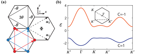
Figure 1: Effective lattice and Chern bands of tMoTe₂. (a) Honeycomb lattice with sublattices $A$ ($B$) in red (blue). The arrows denote the second-neighbor hopping $e^{i\theta_{\sigma}^{\,e}}$ in Eq. (1). Time-reversal symmetry flips spin and arrow directions. Haldane $(\theta)$ and Chern-Simons fluxes $(\Phi=\Phi_{0}\cdot p/q)$ along $+z$ direction are shown; (b) Energy bands of Hamiltonian (1) after particle-hole transformation (2) with $\theta_{\sigma}^{\,h}=-2\pi/3$, $t_{0}=-1$, and $t_{1}=-0.2$: the lower (upper) band carries Chern number $C=1$($-1$); band gap $\Delta E=1.8$.

To characterize FCIs at hole filling $\nu_{\,\text{h}}$ of the highest valence bandCai et al. (2023); Zeng et al. (2023); Park et al. (2023); Xu et al. (2023), we perform a particle-hole (PH) transformation $c_{\ell\sigma}\rightarrow c^{\dagger}_{\ell\sigma}$ that maps the parameters of (1) to

$$\{-t_{0},-t_{1},\theta_{\sigma}^{\,e}\}\xrightarrow{\text{PH}}\{t_{0},t_{1},-\theta^{\,e}_{\sigma}\}\,,$$ (2)

which yields a tight-binding model for holes with hopping parameters $t_{0},t_{1}$ and phase $\theta_{\sigma}^{\,h}=-\theta_{\sigma}^{\,e}=2\pi\sigma/3$. Fig. 1(b) shows the valley-polarized bands for holes with Chern numbers $C=\pm 1$, for $t_{0}=-1$ and $t_{1}=-0.2$, consistent with Ref.Wu et al. (2019) (see also Par ), with the partial filling $0<\nu_{\,\text{h}}<1$ of the lowest band being the subject of this work.

We characterize the onset of incompressible states at partial band filling via a Chern-Simons flux attachment that maps a partially filled Chern band into a set of filled CF bands Möller and Cooper (2015); Murthy and Shankar (2012); Sohal et al. (2018); Wang and Santos (2020). Restricting analysis to uniform particle density states with two Chern-Simons flux quanta (2$\Phi_{0}$) per electron results in the uniform flux per unit cell $\Phi$ (see Fig. 1(a)) proportional to the electron lattice filling $n\in[0,1]$ (or the electron band filling $\nu_{\,\text{e}}=2n\in[0,2]$),

$$\Phi/\Phi_{0}=2\cdot 2n=2\nu_{\,\text{e}}=2\,(2-\nu_{\,\text{h}})\,,$$ (3)

where the coefficient of $n$ in the first equality of Eq. (3) represents the product of 2 fluxes and 2 sublattices, and the last equality follows from charge conservation $\nu_{\,\text{e}}+\nu_{\,\text{h}}=2$. We emphasize that, although we analyze the onset of incompressible CF states by examining the Hofstadter spectrum of holes as a function of filling $0<\nu_{\,\text{h}}<1$, it is important to note that Chern-Simons flux attachment is performed on electrons, not on holes. This distinction is crucial because flux attachment to electrons accurately captures the FCI states observed in experiments, as we will discuss further. Additionally, we have verified that the Hofstadter spectrum of electrons exhibits the same Jain sequence at the corresponding electron filling $1<\nu_{\text{e}}<2$.

The Chern-Simons field is incorporated into $H_{\sigma=-1}$ in Eq. (1) using the Peierls substitution

$$t_{{\bm{r}},{\bm{r}}^{\prime}}\,c^{\dagger}_{{\bm{r}}}c_{{\bm{r}}^{\prime}}\rightarrow t_{{\bm{r}},{\bm{r}}^{\prime}}\,e^{i(2\pi/\Phi_{0})\int^{{\bm{r}}}_{{\bm{r}}^{\prime}}d{\bm{l}}\cdot{\bm{A}}}\,c^{\dagger}_{{\bm{r}}}c_{{\bm{r}}^{\prime}}\,,$$ (4)

where ${\bm{A}}$ is the Chern-Simons vector potential in the gauge ${\bm{A}}=\frac{\Phi}{3\sqrt{3}/2}(x+\sqrt{3}y)\,\hat{e}_{y}$. More details are provided in the Supplemental MaterialsSup .

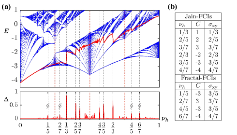
Figure 2: Composite fermion spectrum and emergent FCIs for $\theta_{\sigma}^{\,h}=-2\pi/3$, $t_{0}=-1,t_{1}=-0.2$. (a) Upper part: Hofstadter spectrum $E$ versus $\nu_{\,\text{h}}$, with the red curve showing the Fermi energy. Lower part: The composite fermion gap $\Delta$. Red dashed lines show compressible states at the $1/4,1/2,3/4$ hole fillings; (b) Fractional Hall conductance: table of Jain-FCI and fractal-FCI states at hole band filling $\nu_{\,\text{h}}$.

For rational Chern-Simons flux $\Phi/\Phi_{0}=p/q$ (with $p$ and $q$ coprime), the $C=\pm 1$ bands splits into $2q$ CF bands, resulting in the Hofstadter spectrum of CFs shown in Fig. 2(a). This spectrum has $\Phi\rightarrow\Phi+6\Phi_{0}$ periodicity since the smallest triangle subunit pierced by flux shown in Fig. 1(a) is $1/6$ of the unit cell area. We observe incompressible CF states, indicated by vertical jumps in the composite fermion Fermi energies (red line in Fig. 2(a)) whenever integer bands are filled. This identifies composite fermion gaps $\Delta$ as a function of hole filling $\nu_{\,\text{h}}$.

The Chern number $C\in\mathbb{Z}$ Thouless et al. (1982) of the CF insulator is related to the Hall conductance of asMöller and Cooper (2015); Sup

$$\sigma_{\text{xy}}={C}/{(2C+1)}.$$ (5)

Applying Eqs. (3) and (5) to CF gaps shown in Fig. 2(a), uncovers two classes of candidate FCIs in tMoTe₂. First, we identify states where $\sigma_{\text{xy}}=\nu_{\,\text{h}}\,\frac{e^{2}}{h}$, dubbed Jain-FCI states for the analogy to hierarchical Jain states Jain (1989); Lopez and Fradkin (1991) in Landau level systems. Alternatively, we also identify fractal-FCI states with $\sigma_{\text{xy}}\neq\nu_{\,\text{h}}\,\frac{e^{2}}{h}$ originating from gapped fractal bands distinct from Landau levels.

In Fig. 2(a) and the upper part of Fig. 2(b), we depict a series of Jain-FCI states for hopping parameters $t_{0}=-1$ and $t_{1}=-0.2$ following Ref. Wu et al. (2019). Despite recent variations in the spectrum of Chern bands in tMoTe₂ observed in density functional methods Wang et al. (2024); Reddy et al. (2023); Jia et al. (2024), our results are robust for a range of hoppings. The most prominent gaps occur at $\nu_{\,\text{h}}=1/3$ and $\nu_{\,\text{h}}=2/3$, with noted particle-hole asymmetry. Then, the composite fermion gap $\Delta$ decreases starting from the $2/5,3/5$ hole filling towards $\nu_{\,\text{h}}=1/2$. Notably, we identify Jain-FCIs at $\nu_{\,\text{h}}=2/3,3/5$, with the same topological properties as those recently observed Cai et al. (2023); Zeng et al. (2023); Park et al. (2023); Xu et al. (2023). The CF approach predicts a significant $\nu_{\,\text{h}}=1/3$ gap, but experimental evidence for this FCI remains elusive, possibly due to competing states.

The Jain-FCI sequence extends and converges to a composite Fermi liquid at half-filling. Outside this region, we identify fractal-FCI states shown in the lower part of Fig. 2(b). These originate from the fractal nature of the CF spectrum and possess gaps significantly smaller than most of the Jain-FCI gaps, e.g. at $\nu_{\,\text{h}}=2/3$ and $\nu_{\,\text{h}}=3/5$. This indicates that observing fractal-FCIs may necessitate more stringent conditions, such as lower temperatures or higher sample quality.

Quantum Phase Transitions– We now shift our attention to the states at half-filling ($\nu_{\,\text{h}}=1/2$), to which the Jain sequence converges. The Chern-Simons flux per unit cell at $\nu_{\,\text{h}}=1/2$ is $\Phi=3\Phi_{0}$ (see Eq.3), and to gain generality, we treat the Haldane phase as an independent variable $\theta$. Then the compressible CF states are described by the Hamiltonian $H_{\nu_{\,\text{h}}=1/2}=h_{0}({\bm{k}})\sigma_{0}+\sum^{3}_{i=1}h_{i}({\bm{k}})\sigma_{i}$, with

$$\begin{split}&\,h_{0}({\bm{k}})=2t_{1}\cos\theta\left(\cos k_{1}-\cos k_{2}+\cos(k_{1}-k_{2})\right)\,,\\ &\,h_{1}({\bm{k}})=t_{0}(1-\cos k_{1}+\cos k_{2})\,,\\ &\,h_{2}({\bm{k}})=t_{0}(-\sin k_{1}+\sin k_{2})\,,\\ &\,h_{3}({\bm{k}})=2t_{1}\sin\theta\left(-\sin k_{1}-\sin k_{2}+\sin(k_{1}-k_{2})\right)\,,\end{split}$$ (6)

where $\sigma_{\mu}$ ($\mu=0,1,2,3$) represents the $2\times 2$ identity and three Pauli matrices, and ${\bm{k}}=\frac{k_{1}}{2\pi}{\bm{g}}_{1}+\frac{k_{2}}{2\pi}{\bm{g}}_{2}$ (${\bm{g}}_{1},{\bm{g}}_{2}$ are the reciprocal vectors). The lowest energy band $\varepsilon({\bm{k}})=h_{0}({\bm{k}})-\left({\sum_{i}h^{2}_{i}({\bm{k}})}\right)^{1/2}$ has parabolic dispersion $\varepsilon_{{\bm{p}}}\approx\varepsilon_{0}+{\bm{p}}^{2}/(2m^{*})$ near its minimum with effective mass

$$m^{*}=\frac{m^{*}_{0}}{1+6\,\tau\,\cos{\theta}}\,,$$ (7)

where $m^{*}_{0}=2\hbar^{2}/(3|t_{0}|)$ and $\tau=t_{1}/|t_{0}|$.

An intuitive account of the Jain-FCI states then follows. From Eq. (3), a small change $\delta\nu_{\,\text{h}}=\nu_{\,\text{h}}-1/2$ away from half-filling is connected to a perturbation in the Chern-Simons field $\delta B$,

$$\delta\nu_{\,\text{h}}=\frac{1}{2}\delta\Phi/\Phi_{0}=\frac{1}{2}\delta B\cdot\mathcal{A}_{u.c.}/\Phi_{0}$$ (8)

where $\mathcal{A}_{u.c.}=\frac{3\sqrt{3}}{2}$ is the unit cell area. This extra field $\delta B$, in turn, gives rise to a Landau fan with characteristic energy splitting

$$\Delta_{\textbf{LL}}=\hbar\frac{e\,\delta B}{m^{*}}=\frac{2\Phi_{0}}{\mathcal{A}_{u.c.}}\frac{\hbar e}{m^{*}}\left|\nu_{\,\text{h}}-1/2\right|\,.$$ (9)

This Landau fan structure is clearly seen in Fig. 2(a), and Eq. (9) provides the correct energy scales as $\nu_{\,\text{h}}\rightarrow\frac{1}{2}$ Sup . Furthermore, according to Eq. (9), $\Delta_{\textbf{LL}}\rightarrow 0$ as $m^{*}\rightarrow\infty$, when the band curvature vanishes near the minimum, signaling the onset of a higher order Van Hove singularity (HOVHS)Shtyk et al. (2017); Yuan et al. (2019), which forms along the $\tau\cos{\theta}=-1/6$ curves shown in Fig. 3(a), where the denominator of Eq. (7) vanishes. Except for $\theta=\pm\pi/2$, a HOVHS occurs for a certain finite ratio of first and second neighbor hopings; for tMoTe₂ with $\theta=-2\pi/3$, this occurs for $\tau=1/3$, shown in the solid vertical line in Fig. 3(a).

Fig. 3(b) displays the Hofstadter spectrum at the HOVHS for $\tau_{\textrm{\tiny{HOVHS}}}=1/3$, where a significant reduction in gaps in the range $\nu_{\,\text{h}}=1/3,2/5\ldots,3/5$ is observed, associated with the collapsing of the scale $\Delta_{\textbf{LL}}$.

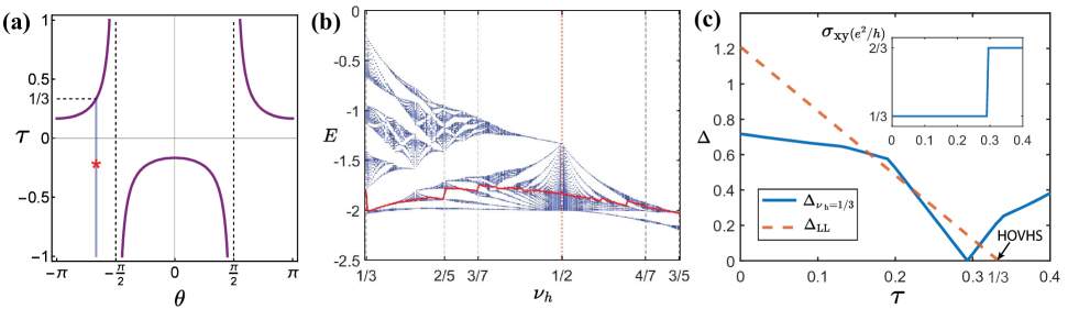
Figure 3: QPT correlated with the HOVHS at $\nu_{\,\text{h}}=1/2$. (a) Curve shows the boundaries where the inverse of effective mass at $\nu_{\,\text{h}}=1/2$ is 0, as a function of $\theta$ and $\tau=t_{1}/|t_{0}|$, the star symbol indicates the set of $\theta,\tau$ used in Fig. 2(a); (b) The Hofstadter spectrum at $t_{0}=-1,\tau=1/3$ and $\theta=-2\pi/3$, zoomed in to show that the composite fermion gaps are nearly closed; (c) The composite fermion gap versus $\tau$: the blue curve represents the gap at $\nu_{\,\text{h}}=1/3$, while the orange dashed line represents the gap (9) predicted by the effective mass approach. This gap vanishes at $\tau=1/3$ as the HOVHS emerges. The inset plots the transition of the Hall conductance $\sigma_{\text{xy}}$.

This feature captures the influence of lattice effects on the structure of CFs in Chern bands, in stark contrast with Landau levels Halperin et al. (1993); Son (2015). While the role of HOVHS in promoting competing electronic orders in Chern bands has been recently emphasizedCastro et al. (2023); Aksoy et al. (2023); Pullasseri and Santos (2024); Wu et al. (2023), to our knowledge, the connection between HOVHS and CF states has not received earlier consideration, and is one of the central results of this work.

Remarkably, the proximity to a HOVHS provides a scenario to explore QPTs induced by closing of the topological gap due to lattice effects. To test this scenario, we plot in Fig. 3(c) the CF gap of the $\nu_{\,\text{h}}=1/3$ state as a function of $\tau$ for $\theta=-2\pi/3$ and $t_{0}=-1$. Near $\tau_{\textrm{\tiny{HOVHS}}}=1/3$, we observe the $\nu_{\,\text{h}}=1/3$ gap following a trend similar to that predicted by Eq. (9), with the gap closing around $\tau\approx 0.3$. The inset shows that this gap closing marks a QPT between a Jain-FCI (C = 1) and a fractal-FCI (C = -2) state with Hall conductances $e^{2}/3h$ and $2e^{2}/3h$, respectively. We have also observed similar QPTs for other FCI states such as $\nu_{\,\text{h}}=2/5,3/7$, confirming the generality of the quantum criticality in proximity to a HOVHS.Sup

We stress that topological phase transitions between CF states can take place outside the HOVHS mechanism discussed above. In fact, an important case occurs at $\nu_{\,\text{h}}=2/3$, which does not follow the Landau fan emanating from the compressible state at half-filling. In Fig. 4, we trace the CF gap and Hall conductance at $\nu_{\,\text{h}}=2/3$ in a wide range of $\tau$. QPTs are observed at multiple ratios $\tau=t_{1}/|t_{0}|$. Notably, for $-0.74<\tau<-0.08$, the incompressible state is a Jain-FCI with Hall conductance $2{e^{2}}/3h$ topologically consistent with experiments.Cai et al. (2023); Zeng et al. (2023); Park et al. (2023); Xu et al. (2023) Furthermore, our analysis predicts that interesting behavior may emerge at $\tau\approx-0.08$ due to competition between distinct FCI states, opening new opportunities for experimental and numerical investigations.

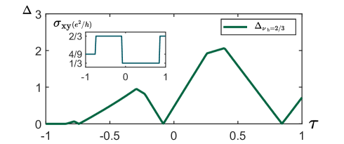
Figure 4: Composite fermion gap $\Delta$ as a function of $\tau$ at $\nu_{\,\text{h}}=2/3$ showing phase transitions at $\Delta=0$. $\theta=-2\pi/3,t_{0}=-1$. The inset plots the phase transition of $\sigma_{\text{xy}}$. The domain of $\sigma_{\text{xy}}=2/3$ ($\sigma_{\text{xy}}=1/3$) corresponds to $-0.74<\tau<-0.08$ ($-0.08<\tau<0.84$).

Discussion– In summary, employing a composite fermion theory, we have characterized the topological properties of fractional Chern insulators in tMoTe₂. In addition to the experimentally observed FCI states at $2/3$ and $3/5$ fillings, our approach reveals several other candidate FCI states, suggesting new pathways to realize topologically ordered phases sans external magnetic fields. We highlight the influence of lattice effects on the stability of fractal CF states and their role in inducing quantum phase transitions through higher-order Van Hove singularities. Expanding this approach to characterize FCIs in multilayer graphene heterostructures Lu et al. (2024) is a promising avenue. Furthermore, a time-reversal symmetric generalization of the composite fermion approach can shed light on the experimental evidenceKang et al. (2024) for the fractional quantum spin Hall effect Bernevig and Zhang (2006); Levin and Stern (2009); Santos et al. (2011); Neupert et al. (2011b) in moiré tMoTe₂. We leave these open questions for future investigation.

Acknowledgments– We are grateful to Andrei Bernevig, Jainendra Jain, and Nicolas Regnault for stimulating discussions. This research was supported by the U.S. Department of Energy, Office of Science, Basic Energy Sciences, under Award DE-SC0023327.

Sec. I describes the Haldane Hamiltonian for the two top bands of tMoTe₂. In Sec. II, we derive the effective Hamiltonian coupled to the Chern-Simons gauge field. Sec. III discussed the Chern-Simons theory of flux attachment and its relation to composite fermions. In Sec. IV, we provide details of the analytical calculation of the effective mass at half-filling ($\nu_{\,\text{h}}=1/2$), and perform linear regression on the Hofstadter spectrum close to half-filling. Furthermore, we provide two more examples of Fig. 3(c) at $\nu_{\,\text{h}}=2/5,3/7$.

I Effective Hamiltonian in the real space

We chose nearest neighbor vectors to be ${\bm{\xi}}_{1}=a(1,0)$, ${\bm{\xi}}_{2}=a(-1/2,+\sqrt{3}/2)$, ${\bm{\xi}}_{3}=a(-1/2,-\sqrt{3}/2)$. Henceforth, $a=1$. The primitive vectors of the Bravais lattice are ${\bm{a}}_{1}={\bm{\xi}}_{1}-{\bm{\xi}}_{2}=(3/2,-\sqrt{3}/2)$ and ${\bm{a}}_{2}={\bm{\xi}}_{1}-{\bm{\xi}}_{3}=(3/2,\sqrt{3}/2)$. The lattice vectors are thus ${\bm{r}}=m\,{\bm{a}}_{1}+n\,{\bm{a}}_{2}$ with $m,n\in\mathbb{Z}$. We arrange the honeycomb lattice such that $A_{m,n}=\psi_{{\bm{r}}=m\,{\bm{a}}_{1}+n\,{\bm{a}}_{2}}$ and $B_{m,n}=\psi_{{\bm{r}}+{\bm{t}}_{1}=m\,{\bm{a}}_{1}+n\,{\bm{a}}_{2}+{\bm{t}}_{1}}$., as shown in the Fig. S1.

Figure S1: Left: arrows indicate direction of hopping (i.e. towards site $A_{m,n}$) and the Peierls phase accumulated. Right: arrows indicate direction of NNN hopping amplitude $t_{1}e^{i\theta}$. The accumulated Peierls phase in along the NNN hopping can be directly obtained from the phases on the left and the fact that the Aharonov-Bohm phase experience by a charged particle is $e^{\pm i2\pi\phi_{triangle}/\phi_{0}}$ where $\pm$ indicates CCW/CW dirctions and $\phi_{triangle}=\phi_{0}/6$ is the flux in a triangle that has a blue arrow as one of the edges.

I.1 Two-band Haldane model

The model contains a NN hopping of strength $t_{0}$ and a complex hopping $t_{1}\,e^{i\theta}$ as indicated in Fig. S1 (right),

$$H=H_{0}+H_{1}\equiv H_{0}+H_{AA}+H_{BB}\,,$$ (S1)

where

$$H_{0}=t_{0}\,\sum_{m,n}\Big{(}A^{\dagger}_{m,n}\,B_{m,n}+A^{\dagger}_{m,n}\,B_{m-1,n}+A^{\dagger}_{m,n}\,B_{m,n-1}\Big{)}+\textrm{H.c.}\,,$$ (S2)

$$H_{AA}=t_{1}\,e^{i\theta}\,\sum_{m,n}\Big{(}A^{\dagger}_{m,n+1}A_{m,n}+A^{\dagger}_{m-1,n}A_{m,n}+A^{\dagger}_{m+1,n-1}A_{m,n}\Big{)}+\textrm{H.c.}\,$$ (S3)

and

$$H_{BB}=t_{1}\,e^{i\theta}\,\sum_{m,n}\Big{(}B^{\dagger}_{m-1,n+1}B_{m,n}+B^{\dagger}_{m,n-1}B_{m,n}+B^{\dagger}_{m+1,n}B_{m,n}\Big{)}+\textrm{H.c.}\,.$$ (S4)

Defining the Fourier transform of the fermionic operators as

$$A_{{\bm{r}}}\equiv A_{m,n}=\frac{1}{\sqrt{N}}\sum_{{\bm{k}}\in BZ}\,e^{i{\bm{k}}\cdot{\bm{r}}}A_{{\bm{k}}}\,,\quad B_{{\bm{r}}}\equiv B_{m,r}=\frac{1}{\sqrt{N}}\sum_{{\bm{k}}\in BZ}\,e^{i{\bm{k}}\cdot{\bm{r}}}B_{{\bm{k}}}\,,$$ (S5)

leads to

$$H_{0}=\sum_{{\bm{k}}}A^{\dagger}_{{\bm{k}}}B_{{\bm{k}}}\,t_{0}(1+e^{-ik_{1}}+e^{-ik_{2}})+\textrm{H.c.}\,,$$ (S6)

$$H_{AA}=\sum_{{\bm{k}}}A^{\dagger}_{{\bm{k}}}A_{{\bm{k}}}\,t_{1}e^{i\theta}(e^{-ik_{2}}+e^{ik_{1}}+e^{i(-k_{1}+k_{2})})+\textrm{H.c.}$$ (S7)

$$H_{BB}=\sum_{{\bm{k}}}B^{\dagger}_{{\bm{k}}}B_{{\bm{k}}}\,t_{1}e^{i\theta}(e^{ik_{2}}+e^{-ik_{1}}+e^{i(k_{1}-k_{2})})+\textrm{H.c.}$$ (S8)

All in all, the model is written as

$$H=\sum_{{\bm{k}}}\begin{pmatrix}A^{\dagger}_{{\bm{k}}}&B^{\dagger}_{{\bm{k}}}\end{pmatrix}\,\begin{pmatrix}t_{1}e^{i\theta}(e^{-ik_{2}}+e^{ik_{1}}+e^{i(-k_{1}+k_{2})})+\textrm{c.c.}&t_{0}(1+e^{-ik_{1}}+e^{-ik_{2}})\\ t_{0}(1+e^{ik_{1}}+e^{ik_{2}})&t_{1}e^{i\theta}(e^{ik_{2}}+e^{-ik_{1}}+e^{i(k_{1}-k_{2})})+\textrm{c.c.}\end{pmatrix}\begin{pmatrix}A_{{\bm{k}}}\\ B_{{\bm{k}}}\end{pmatrix}$$ (S9)

II Hofstadter bands

Perpendicular to the plane of the lattice we consider is a uniform Chern-Simons field ${\bm{B}}={\bm{\nabla}}\times{\bm{A}}$ and we adopt the gauge ${\bm{A}}=B(x+\sqrt{3}y)\vec{e}_{y}$. The area of the unit cell is $A_{u.c.}=3\sqrt{3}/2$ which gives a flux $\phi=B\,3\sqrt{3}/2$. With $B$ in the positive direction, this gives a positive counter-clockwise phase $e^{i(q/\hbar)\oint d{\bm{l}}\cdot{\bm{A}}}=e^{i(q/\hbar)\phi}=e^{i2\pi\phi/\phi_{0}}$, where $\phi_{0}=q/h$. Henceforth, we define $\omega=e^{i2\pi\phi/\phi_{0}}$ and we will be considering the case where $\phi/\phi_{0}=p/q$ is a rational number.

We describe the effect of the Chern-Simons gauge field via a Peierls substitution according to

$$t_{{\bm{r}},{\bm{r}}^{\prime}}\,\psi^{\dagger}_{{\bm{r}}}\psi_{{\bm{r}}^{\prime}}\rightarrow t_{{\bm{r}},{\bm{r}}^{\prime}}\,e^{i(2\pi/\phi_{0})\int^{{\bm{r}}}_{{\bm{r}}^{\prime}}d{\bm{l}}\cdot{\bm{A}}}\,\psi^{\dagger}_{{\bm{r}}}\psi_{{\bm{r}}^{\prime}}\,.$$ (S10)

II.1 Nearest neighbor hopping

Fig. S1 (left) shows the Peiers phases accumulated a charged particle that hops into the $A_{m,n}$ site from its nearest neighbor B sites. This leads to the tight-binding Hamiltonian

$$H_{0}=t_{0}\,\sum_{m,n}\Big{(}A^{\dagger}_{m,n}\,B_{m,n}+\omega^{-1/6-n}\,A^{\dagger}_{m,n}\,B_{m-1,n}+\omega^{-1/3+n}\,A^{\dagger}_{m,n}\,B_{m,n-1}\Big{)}+\textrm{H.c.}$$ (S11)

We see that the Hamiltonian has an effective translation symmetry $(m,n)\rightarrow(m+1,n+q)$, which embodies the magnetic translation symmetry of the Hamiltonian in the presence of an external magnetic field. Naturally, we extend the unit cell along the ${\bm{a}}_{2}$ direction such that the system has a magnetic unit cell with $2\times q$ sites and the primitive lattice vectors are ${\bm{a}}^{{}^{\prime}}_{1}={\bm{a}}_{1}$ and ${\bm{a}}^{{}^{\prime}}_{2}=q\,{\bm{a}}_{2}$. Accordingly, we define reciprocal lattice vectors of the magnetic BZ as ${\bm{g}}^{{}^{\prime}}_{1}$ and ${\bm{g}}^{{}^{\prime}}_{2}$ via ${\bm{a}}^{{}^{\prime}}_{i}\cdot{\bm{g}}^{{}^{\prime}}_{j}=2\pi\delta_{ij}$, and parameterized momentum via ${\bm{k}}=k_{1}{\bm{g}}^{{}^{\prime}}_{1}+k_{2}{\bm{g}}^{{}^{\prime}}_{2}$.

Letting $n=q\,r+s$ with $r\in\mathbb{Z}$ and $s=0,...,q-1$, we introduce subalttice operators as

$$A_{m,n}=A_{m,q\,r+s}\equiv A^{(s)}_{m,r}\equiv A^{(s)}_{{\bm{R}}}\,,\quad B_{m,n}=B_{m,q\,r+s}\equiv B^{(s)}_{m,r}\equiv B^{(s)}_{{\bm{R}}}\,,$$ (S12)

where ${\bm{R}}=m{\bm{a}}^{{}^{\prime}}_{1}+r{\bm{a}}^{{}^{\prime}}_{2}$ is the position of the magnetic unit cell, and their Fourier transforms

$$A^{(s)}_{m,r}=\frac{1}{\sqrt{N}}\sum_{{\bm{k}}\in MBZ}\,e^{i{\bm{k}}\cdot{\bm{R}}}A^{(s)}_{{\bm{k}}}\,,\quad B^{(s)}_{m,r}=\frac{1}{\sqrt{N}}\sum_{{\bm{k}}\in MBZ}\,e^{i{\bm{k}}\cdot{\bm{R}}}B^{(s)}_{{\bm{k}}}$$ (S13)

and express each of the terms of the Hamiltonian (S11) as

$$X_{1}=\sum_{m,n}A^{\dagger}_{m,n}\,B_{m,n}=\sum_{m,r}\sum^{q-1}_{s=0}\,(A^{s}_{m,r})^{\dagger}\,B^{s}_{m,r}=\sum_{{\bm{k}}}\sum^{q-1}_{s=0}\,(A^{s}_{{\bm{k}}})^{\dagger}\,B^{s}_{{\bm{k}}}\,,$$ (S14)

$$X_{2}=\sum_{m,n}\omega^{-1/6-n}A^{\dagger}_{m,n}\,B_{m-1,n}=\sum_{m,r}\sum^{q-1}_{s=0}\,\omega^{-1/6-s}(A^{s}_{m,r})^{\dagger}\,B^{s}_{m-1,r}=\sum_{{\bm{k}}}\sum^{q-1}_{s=0}\,\omega^{-1/6-s}e^{-ik_{1}}(A^{s}_{{\bm{k}}})^{\dagger}\,B^{s}_{{\bm{k}}}\,,$$ (S15)

and

$$\begin{split}X_{3}&\,=\sum_{m,n}\omega^{-1/3+n}\,A^{\dagger}_{m,n}\,B_{m,n-1}=\sum_{m,r}\sum^{q-1}_{q=0}\omega^{-1/3+s}\,A^{\dagger}_{m,qr+s}\,B_{m,qr+s-1}\\ &\,=\sum_{m,r}\Big{[}\omega^{-1/3}\,A^{\dagger}_{m,qr}\,B_{m,qr-1}+\sum^{q-1}_{q=1}\omega^{-1/3+s}\,A^{\dagger}_{m,qr+s}\,B_{m,qr+s-1}\Big{]}\\ &\,=\sum_{m,r}\Big{[}\omega^{-1/3}\,(A^{(0)}_{m,r})^{\dagger}\,B^{(q-1)}_{m,r-1}+\sum^{q-1}_{q=1}\omega^{-1/3+s}\,(A^{(s)}_{m,r})^{\dagger}\,B^{(s-1)}_{m,r}\Big{]}\\ &\,=\sum_{{\bm{k}}}\Big{[}\omega^{-1/3}\,e^{-ik_{2}}(A^{(0)}_{{\bm{k}}})^{\dagger}\,B^{(q-1)}_{{\bm{k}}}+\sum^{q-1}_{q=1}\omega^{-1/3+s}\,(A^{(s)}_{{\bm{k}}})^{\dagger}\,B^{(s-1)}_{{\bm{k}}}\Big{]}\end{split}$$ (S16)

Then the nearest neighbor Hamiltonian $H_{0}=t_{0}\,(X_{1}+X_{2}+X_{3})+\textrm{H.c.}$ then reads

$$\begin{split}H_{0}&\,=t_{0}\sum_{{\bm{k}}}\sum^{q-1}_{s=0}\,(1+\omega^{-1/6-s}e^{-ik_{1}})(A^{s}_{{\bm{k}}})^{\dagger}\,B^{s}_{{\bm{k}}}+\textrm{H.c.}\\ &\,t_{0}\sum_{{\bm{k}}}\Big{[}\omega^{-1/3}\,e^{-ik_{2}}(A^{(0)}_{{\bm{k}}})^{\dagger}\,B^{(q-1)}_{{\bm{k}}}+\sum^{q-1}_{q=1}\omega^{-1/3+s}\,(A^{(s)}_{{\bm{k}}})^{\dagger}\,B^{(s-1)}_{{\bm{k}}}\Big{]}+\textrm{H.c.}\end{split}$$ (S17)

II.2 Next nearest neighbor hopping

The NNN Hamiltonian

$$H_{1}=H_{AA}+H_{BB}$$ (S18)

corresponds to hopping between equal sublattices.

The AA hopping - with the arrows in Fig. S1 (right) indicates the direction with topological hopping $t_{1}e^{i\theta}$ - is given by

$$H_{AA}=t_{1}\,e^{i\theta}\,\sum_{m,n}\Big{(}\omega^{n+1/2}\,A^{\dagger}_{m,n+1}A_{m,n}+\omega^{n}\,A^{\dagger}_{m-1,n}A_{m,n}+\omega^{1-2n}A^{\dagger}_{m+1,n-1}A_{m,n}\Big{)}+\textrm{H.c.}$$ (S19)

Fourier transforming,

$$\begin{split}H_{AA}&\,=t_{1}e^{i\theta}\sum_{{\bm{k}}}\Big{[}\sum^{q-2}_{s=0}\omega^{s+1/2}A^{s+1\dagger}_{{\bm{k}}}A^{s}_{{\bm{k}}}+\omega^{(q-1)+1/2}e^{-ik_{2}}A^{0\dagger}_{{\bm{k}}}A^{q-1}_{{\bm{k}}}\Big{]}\\ &\,+t_{1}e^{i\theta}\sum_{{\bm{k}}}\sum^{q-1}_{s=0}\omega^{s}e^{ik_{1}}A^{s\dagger}_{{\bm{k}}}A^{s}_{{\bm{k}}}\\ &\,+t_{1}e^{i\theta}\sum_{{\bm{k}}}\Big{[}\omega^{1}e^{-ik_{1}+ik_{2}}A^{q-1\dagger}_{{\bm{k}}}A^{0}_{{\bm{k}}}+\sum^{q-1}_{s=1}\omega^{1-2s}e^{-ik_{1}}A^{s-1\dagger}_{{\bm{k}}}A^{s}_{{\bm{k}}}\Big{]}\\ &\,+\textrm{H.c.}\end{split}$$ (S20)

The BB hopping - with the arrows in Fig. S1 (right) indicates the direction with topological hopping $t_{1}e^{i\theta}$ - is given by

$$H_{BB}=t_{1}\,e^{i\theta}\,\sum_{m,n}\Big{(}\omega^{2n+5/3}\,B^{\dagger}_{m-1,n+1}B_{m,n}+\omega^{1/6-n}\,B^{\dagger}_{m,n-1}B_{m,n}+\omega^{-1/3-n}B^{\dagger}_{m+1,n}B_{m,n}\Big{)}+\textrm{H.c.}$$ (S21)

By Fourier transform, we get

$$\begin{split}H_{BB}&\,=t_{1}e^{i\theta}\sum_{{\bm{k}}}\Big{[}\sum^{q-2}_{s=0}\omega^{5/3+2s}e^{ik_{1}}B^{s+1\dagger}_{{\bm{k}}}B^{s}_{{\bm{k}}}+\omega^{5/3+2(q-1)}e^{ik_{1}-ik_{2}}B^{0\dagger}_{{\bm{k}}}B^{q-1}_{{\bm{k}}}\Big{]}\\ &\,+t_{1}e^{i\theta}\sum_{{\bm{k}}}\Big{[}\sum^{q-1}_{s=1}\omega^{1/6-s}B^{s-1\dagger}_{{\bm{k}}}B^{s}_{{\bm{k}}}+\omega^{1/6}e^{ik_{2}}B^{q-1\dagger}_{{\bm{k}}}B^{0}_{{\bm{k}}}\Big{]}\\ &\,+t_{1}e^{i\theta}\sum_{{\bm{k}}}\sum^{q-1}_{s=0}\omega^{-1/3-s}e^{-ik_{1}}B^{s\dagger}_{{\bm{k}}}B^{s}_{{\bm{k}}}\\ &\,+\textrm{H.c.}\end{split}$$ (S22)

III Chern-Simons theory of flux attachment

The composite fermion theory characterizes an incompressible state of a partially filled topological band in terms of a band insulator of composite fermions, which are bound states of an electron (or hole) and an even number $2p$ of flux quanta $\phi_{0}=h/e=2\pi$ (in units where $\hbar=e=1)$.

To accomplish the flux attachment, we introduce a Chern-Simons statistical gauge field $a_{\mu}$ and impose the condition

$$(2p)\,J^{\mu}=\frac{1}{2\pi}\varepsilon^{\mu\nu\lambda}\partial_{\nu}a_{\lambda}\,,$$ (S23)

where $J^{\mu}$ is the number current density. To understand the significance of Eq. S23, consider the $\mu=0$ equation

$$(2p)\,J^{0}=\frac{1}{2\pi}\varepsilon^{0ij}\partial_{i}a_{j}\,,$$ (S24)

where $J^{0}$ is the number density. Integrating over space and using Stoke’s equation

$$(2p)\,\int d^{2}{\bm{r}}J^{0}=\frac{1}{2\pi}\int d^{2}{\bm{r}}\varepsilon^{0ij}\partial_{i}a_{j}=\frac{1}{2\pi}\oint{\bm{a}}\cdot d{\bm{\ell}}\,.$$ (S25)

Since the right hand side gives the Chern-Simons flux divided by the flux quantum (recall $\phi_{0}=2\pi$), this equation establishes that each particle is attached to $2p$ flux quanta.

It turns out that Eq. S23 can be obtained as the Euler-Lagrange equation of motion of a local field theory as follows. First, because $J^{\mu}$ is a conserved current, that is $\partial_{\mu}J^{\mu}=0$, it can be expressed in terms of the gradient of a gauge field $b_{\mu}$ as follows,

$$J^{\mu}\equiv\frac{1}{2\pi}\varepsilon^{\mu\nu\lambda}\partial_{\nu}b_{\lambda}\,.$$ (S26)

Eq. S26 describes a particle-vortex duality transformation in $(2+1)$ dimensions.

Consider now the action

$$S_{1}=\int d^{3}x\mathcal{L}=\int d^{3}x\Big{(}-\frac{2p}{4\pi}\varepsilon^{\mu\nu\lambda}b_{\mu}\partial_{\nu}b_{\lambda}+\frac{1}{2\pi}\varepsilon^{\mu\nu\lambda}a_{\mu}\partial_{\nu}b_{\lambda}\Big{)}$$ (S27)

Then, it is straightforward to verify that

$$\frac{\delta S_{1}}{\delta b_{\mu}}=0\quad\Leftrightarrow\quad\frac{2p}{2\pi}\varepsilon^{\mu\nu\lambda}\partial_{\nu}b_{\lambda}=\frac{1}{2\pi}\varepsilon^{\mu\nu\lambda}\partial_{\nu}a_{\lambda}\,,$$ (S28)

which is the flux attachment condition Eq. S23.

Now, we write general action that contains fermions and the gauge fields

$$S_{2}=\int d^{3}x\mathcal{L}=\int d^{3}x\Big{(}\mathcal{L}(\psi^{\dagger},\psi,a_{\mu})-\frac{2p}{4\pi}\varepsilon^{\mu\nu\lambda}b_{\mu}\partial_{\nu}b_{\lambda}+\frac{1}{2\pi}\varepsilon^{\mu\nu\lambda}a_{\mu}\partial_{\nu}b_{\lambda}\Big{)}\,$$ (S29)

where $\mathcal{L}(\psi^{\dagger},\psi,a_{\mu})$ is the Lagrangian describing fermions coupled to the statistical gauge field $a_{\mu}$. When fermions forms a gapped insulator state, integrating out fermions results in a universal Chern-Simons response

$$S_{3}=\int d^{3}x\mathcal{L}=\int d^{3}x\Big{(}\frac{C}{4\pi}\varepsilon^{\mu\nu\lambda}a_{\mu}\partial_{\nu}a_{\lambda}-\frac{2p}{4\pi}\varepsilon^{\mu\nu\lambda}b_{\mu}\partial_{\nu}b_{\lambda}+\frac{1}{2\pi}\varepsilon^{\mu\nu\lambda}a_{\mu}\partial_{\nu}b_{\lambda}\Big{)}\,$$ (S30)

where $C$ is the Chern-number of the fermionic insulator, which in this case is the Chern number of the composite fermion state.

To probe this state’s response, we turn on an external probe field $A_{\mu}$ minimally coupled to the charge current $q\,J^{\mu}$ ($q=-e$ for the electron) by adding the term $-J^{\mu}A_{\mu}=-\,\frac{1}{2\pi}\varepsilon^{\mu\nu\lambda}A_{\mu}\partial_{\nu}b_{\lambda}$, which results in the action

$$S_{4}=\int d^{3}x\mathcal{L}=\int d^{3}x\Big{(}\frac{C}{4\pi}\varepsilon^{\mu\nu\lambda}a_{\mu}\partial_{\nu}a_{\lambda}-\frac{2p}{4\pi}\varepsilon^{\mu\nu\lambda}b_{\mu}\partial_{\nu}b_{\lambda}+\frac{1}{2\pi}\varepsilon^{\mu\nu\lambda}a_{\mu}\partial_{\nu}b_{\lambda}-\frac{1}{2\pi}\varepsilon^{\mu\nu\lambda}A_{\mu}\partial_{\nu}b_{\lambda}\Big{)}\,$$ (S31)

We introduce a two-component gauge field

$$a^{I}_{\mu}=\begin{pmatrix}b_{\mu}\\ a_{\mu}\end{pmatrix}\,,$$ (S32)

and express the action as

$$S_{4}=\int d^{3}x\mathcal{L}=\int d^{3}x\Big{(}\frac{1}{4\pi}K_{IJ}\varepsilon^{\mu\nu\lambda}a^{I}_{\mu}\partial_{\nu}a^{J}_{\lambda}-Q_{I}\,\frac{1}{2\pi}\varepsilon^{\mu\nu\lambda}A_{\mu}\partial_{\nu}a^{I}_{\lambda}\Big{)}\,$$ (S33)

where

$$K=\begin{pmatrix}-2p&1\\ 1&C\end{pmatrix}\,,\quad Q=\begin{pmatrix}1\\ 0\end{pmatrix}$$ (S34)

are, respectively, the symmetric K-matrix and the charge vector.

Integrating out $a^{I}$ fields gives the response action for the external probe field

$$S_{eff}=\int d^{3}x\mathcal{L}=-Q^{T}\cdot K^{-1}\cdot Q\int d^{3}x\frac{1}{4\pi}\varepsilon^{\mu\nu\lambda}A_{\mu}\partial_{\nu}A_{\lambda}\,.$$ (S35)

From $J^{\mu}=\frac{\delta S_{eff}}{\delta A_{\mu}}$, one recovers the Hall conductivity

$$\sigma_{xy}=\frac{C}{2p\,C+1}\,.$$ (S36)

IV Composite fermion gaps correlated with emergent HOVHS

IV.1 Effective mass

At half-filling ($\nu_{\,\text{h}}=1/2$), $p=3,q=1$, the Hamiltonian is $2\times 2$. The nearest neighbor Hamiltonian reads

$$\begin{split}H_{0}&\,=t_{0}\sum_{{\bm{k}}}\sum^{q-1}_{s=0}\,(1+\omega^{-1/6-s}e^{-ik_{1}})(A^{s}_{{\bm{k}}})^{\dagger}\,B^{s}_{{\bm{k}}}+\textrm{H.c.}\\ &\,+t_{0}\sum_{{\bm{k}}}\Big{[}\omega^{-1/3}\,e^{-ik_{2}}(A^{(0)}_{{\bm{k}}})^{\dagger}\,B^{(q-1)}_{{\bm{k}}}+\sum^{q-1}_{s=1}\omega^{-1/3+s}\,(A^{(s)}_{{\bm{k}}})^{\dagger}\,B^{(s-1)}_{{\bm{k}}}\Big{]}+\textrm{H.c.}\\ &\,=t_{0}(1+\omega^{-1/6}\,e^{-ik_{1}}+\omega^{-1/3}\,e^{-ik_{2}})A^{\dagger}_{{\bm{k}}}\,B_{{\bm{k}}}+\textrm{H.c.}\end{split}$$ (S37)

The AA-hopping reads

$$\begin{split}H_{AA}&\,=t_{1}e^{i\theta}\sum_{{\bm{k}}}\Big{[}\sum^{q-2}_{s=0}\omega^{s+1/2}A^{s+1\dagger}_{{\bm{k}}}A^{s}_{{\bm{k}}}+\omega^{(q-1)+1/2}e^{-ik_{2}}A^{0\dagger}_{{\bm{k}}}A^{q-1}_{{\bm{k}}}\Big{]}\\ &\,+t_{1}e^{i\theta}\sum_{{\bm{k}}}\sum^{q-1}_{s=0}\omega^{s}e^{ik_{1}}A^{s\dagger}_{{\bm{k}}}A^{s}_{{\bm{k}}}\\ &\,+t_{1}e^{i\theta}\sum_{{\bm{k}}}\Big{[}\omega^{1}e^{-ik_{1}+ik_{2}}A^{q-1\dagger}_{{\bm{k}}}A^{0}_{{\bm{k}}}+\sum^{q-1}_{s=1}\omega^{1-2s}e^{-ik_{1}}A^{s-1\dagger}_{{\bm{k}}}A^{s}_{{\bm{k}}}\Big{]}\\ &\,+\textrm{H.c.}\\ &\,=t_{1}e^{i\theta}(\omega^{1/2}e^{-ik_{2}}+e^{ik_{1}}+\omega e^{-ik_{1}+ik_{2}})A^{\dagger}_{{\bm{k}}}A_{{\bm{k}}}+\textrm{H.c.}\end{split}$$ (S38)

The BB-hopping reads

$$\begin{split}H_{BB}&\,=t_{1}e^{i\theta}\sum_{{\bm{k}}}\Big{[}\sum^{q-2}_{s=0}\omega^{5/3+2s}e^{ik_{1}}B^{s+1\dagger}_{{\bm{k}}}B^{s}_{{\bm{k}}}+\omega^{5/3+2(q-1)}e^{ik_{1}-ik_{2}}B^{0\dagger}_{{\bm{k}}}B^{q-1}_{{\bm{k}}}\Big{]}\\ &\,+t_{1}e^{i\theta}\sum_{{\bm{k}}}\Big{[}\sum^{q-1}_{s=1}\omega^{1/6-s}B^{s-1\dagger}_{{\bm{k}}}B^{s}_{{\bm{k}}}+\omega^{1/6}e^{ik_{2}}B^{q-1\dagger}_{{\bm{k}}}B^{0}_{{\bm{k}}}\Big{]}\\ &\,+t_{1}e^{i\theta}\sum_{{\bm{k}}}\sum^{q-1}_{s=0}\omega^{-1/3-s}e^{-ik_{1}}B^{s\dagger}_{{\bm{k}}}B^{s}_{{\bm{k}}}\\ &\,+\textrm{H.c.}\\ &\,=t_{1}e^{i\theta}(\omega^{5/3}e^{ik_{1}-ik_{2}}+\omega^{1/6}e^{ik_{2}}+\omega^{-1/3}e^{-ik_{1}})B_{{\bm{k}}}^{\dagger}B_{{\bm{k}}}+\textrm{H.c.}\end{split}$$ (S39)

Collecting previous terms leads to the 2x2 Hamiltonian is

$$H[k_{1},k_{2},\theta,t_{0},t_{1}]=\begin{pmatrix}H_{AA}&H_{0}\\ H_{0}^{*}&H_{BB}\end{pmatrix}=h_{0}({\bm{k}})\sigma_{0}+\sum^{3}_{i=1}h_{i}({\bm{k}})\sigma_{i}\,,$$ (S40)

with

$$\begin{split}&h_{0}({\bm{k}})=2t_{1}\cos\theta\left(\cos k_{1}-\cos k_{2}+\cos(k_{1}-k_{2})\right)\\ &h_{1}({\bm{k}})=t_{0}(1-\cos k_{1}+\cos k_{2})\\ &h_{2}({\bm{k}})=t_{0}(-\sin k_{1}+\sin k_{2})\\ &h_{3}({\bm{k}})=2t_{1}\sin\theta\left(-\sin k_{1}-\sin k_{2}+\sin(k_{1}-k_{2})\right)\end{split}\,.$$ (S41)

The energy of the lower band is directly obtained

$$\varepsilon_{-}({\bm{k}})=\frac{H_{AA}+H_{BB}}{2}-\frac{1}{2}\sqrt{(H_{AA}-H_{BB})^{2}+4H_{0}H_{0}^{*}}=h_{0}({\bm{k}})-|{\bm{h}}({\bm{k}})|\,.$$ (S42)

At $k_{1}=-p\cdot\frac{\pi}{3},k_{2}=-p\cdot\frac{2\pi}{3}$, $E_{\text{low}}$ reaches the minimum, i.e.

$$\begin{split}&\partial_{k_{1}}\varepsilon_{-}({\bm{k}})=\partial_{k_{2}}\varepsilon_{-}({\bm{k}})=0\\ &\partial^{2}_{k_{1}}\varepsilon_{-}({\bm{k}})=\partial^{2}_{k_{2}}\varepsilon_{-}({\bm{k}})=\frac{2}{3}|t_{0}|+4t_{1}\cos(\theta)\\ &\partial_{k_{1}}\partial_{k_{2}}\varepsilon_{-}({\bm{k}})=-\frac{1}{3}|t_{0}|-2t_{1}\cos(\theta)\end{split}$$ (S43)

Expanding $\varepsilon_{-}({\bm{k}})$ around the minimum,

$$\varepsilon_{-}({\bm{k}})=\varepsilon^{*}_{-}+\frac{1}{2}\left(\frac{2}{3}|t_{0}|+4t_{1}\cos(\theta)\right)\begin{pmatrix}k_{1}&k_{2}\end{pmatrix}\begin{pmatrix}1&-1/2\\ -1/2&1\end{pmatrix}\begin{pmatrix}k_{1}\\ k_{2}\end{pmatrix}$$ (S44)

Considering $\mathbf{k}=\frac{k_{1}}{2\pi}\vec{g}_{1}+\frac{k_{2}}{2\pi}\vec{g}_{2}$, with $\vec{g}_{1}=\frac{4\pi}{3}(1/2,-\sqrt{3}/2)$ and $\vec{g}_{2}=\frac{4\pi}{3}(1/2,\sqrt{3}/2)$, gives

$$\begin{pmatrix}k_{x}\\ k_{y}\end{pmatrix}=\frac{1}{3}\begin{pmatrix}1&1\\ -\sqrt{3}&\sqrt{3}\end{pmatrix}\begin{pmatrix}k_{1}\\ k_{2}\end{pmatrix}\leftrightarrow\begin{pmatrix}k_{1}\\ k_{2}\end{pmatrix}=\begin{pmatrix}3/2&-\sqrt{3}/2\\ 3/2&\sqrt{3}/2\end{pmatrix}\begin{pmatrix}k_{x}\\ k_{y}\end{pmatrix}$$ (S45)

resulting in the rotationally invariant parabolic expansion

$$\begin{split}\varepsilon_{-}({\bm{k}})&=\varepsilon^{*}_{-}+\frac{1}{2}\left(\frac{2}{3}|t_{0}|+4t_{1}\cos(\theta)\right)\begin{pmatrix}k_{x}&k_{y}\end{pmatrix}\begin{pmatrix}9/4&0\\ 0&9/4\end{pmatrix}\begin{pmatrix}k_{x}\\ k_{y}\end{pmatrix}\end{split}$$ (S46)

from which

$$\varepsilon_{\text{eff}}=\frac{\hbar^{2}}{2m^{*}}k^{2}=\left(\frac{3}{4}|t_{0}|+\frac{9}{2}t_{1}\cos(\theta)\right)k^{2}$$ (S47)

yields the effective mass in Eq. (7).

Following the same approach of Eq. (9), we can approximate the slopes of the energy bands in the Landau-fan asymptotically close to the half-filling($\nu_{\,\text{h}}=1/2$) according to

$$E_{n}=E^{*}+(n+1/2)\hbar\omega_{c}=E^{*}+(n+1/2)\frac{4}{3\sqrt{3}}\Phi_{0}\frac{\hbar e}{m^{*}}|\nu_{\,\text{h}}-1/2|\Rightarrow\mathrm{d}E_{n}/\mathrm{d}\delta\nu_{\,\text{h}}=\pm(n+1/2)\frac{4}{3\sqrt{3}}\Phi_{0}\frac{\hbar e}{m^{*}}$$ (S48)

To compare the slopes in Eq. (S48) with the Hofstadter spectrum, we perform linear regression on the lowest three bands in the Hofstadter spectrum close to the half-filling at $\theta=-2\pi/3,t_{0}=-1,t_{1}=-0.2$ as shown in Fig. S2.

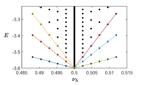
Figure S2: Linear regression of the lowest three bands in the Landau-fan at $\theta=-2\pi/3,t_{0}=-1,t_{1}=-0.2$. Solid dots are the Hofstadter spectrum, solid lines with error bars show the linear regression.

The fitting result compared with Eq. (S48) is summarized in Table. S1, their agreement supports the Landau-fan picture accounted by the effective mass at half-filling.

Landau-fan Slope
Landau level index	Linear regression		Eq. (S48)
	$\nu_{\,\text{h}}<1/2$	$\nu_{\,\text{h}}>1/2$	-
$\Delta E_{0}=(0+1/2)\hbar\omega_{c}$	$-5.7128\pm 0.0107$	$5.7171\pm 0.0099$	$\pm 5.8042$
$\Delta E_{1}=(1+1/2)\hbar\omega_{c}$	$-16.9621\pm 0.0523$	$16.9793\pm 0.0488$	$\pm 17.4125$
$\Delta E_{2}=(2+1/2)\hbar\omega_{c}$	$-27.8583\pm 0.1342$	$27.9012\pm 0.1256$	$\pm 29.0208$

Table S1: The Landau-fan slopes from linear regression and predicted by Eq. (S48) at $\theta=-2\pi/3,t_{0}=-1,t_{1}=-0.2$.

IV.2 QPT correlated with HOVHS for $\nu_{\,\text{h}}=2/5,3/7$

Here we present two more examples of Fig. 3(c) closer to the half-filling at $\nu_{\,\text{h}}=2/5,3/7$ (in Fig. S3) to show that the correlation between QPTs and HOVHS is extensive in the Jain-FCI states.

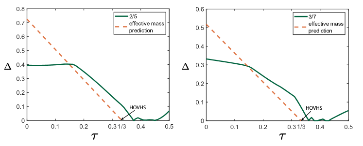
Figure S3: $\sigma=-1,\theta=-2\pi/3,t_{0}=-1$. The composite fermion gap versus $\tau$. left: $\nu_{\,\text{h}}=2/5$, right: $\nu_{\,\text{h}}=3/7$. The green curve shows the gap, the orange line shows the gap predicted for each hole filling by effective mass at $\nu_{\,\text{h}}=1/2$ which vanishes at $\tau=1/3$ as the HOVHS emerges.

References

• Neupert et al. (2011a) T. Neupert, L. Santos, C. Chamon,  and C. Mudry, Phys. Rev. Lett. 106, 236804 (2011a).
• Sheng et al. (2011) D. N. Sheng, Z.-C. Gu, K. Sun,  and L. Sheng, Nature Communications 2, 389 EP (2011).
• Tang et al. (2011) E. Tang, J.-W. Mei,  and X.-G. Wen, Phys. Rev. Lett. 106, 236802 (2011).
• Sun et al. (2011) K. Sun, Z. Gu, H. Katsura,  and S. Das Sarma, Phys. Rev. Lett. 106, 236803 (2011).
• Regnault and Bernevig (2011) N. Regnault and B. A. Bernevig, Phys. Rev. X 1, 021014 (2011).
• Cai et al. (2023) J. Cai, E. Anderson, C. Wang, X. Zhang, X. Liu, W. Holtzmann, Y. Zhang, F. Fan, T. Taniguchi, K. Watanabe, et al., Nature 622, 63 (2023).
• Zeng et al. (2023) Y. Zeng, Z. Xia, K. Kang, J. Zhu, P. Knüppel, C. Vaswani, K. Watanabe, T. Taniguchi, K. F. Mak,  and J. Shan, Nature 622, 69 (2023).
• Park et al. (2023) H. Park, J. Cai, E. Anderson, Y. Zhang, J. Zhu, X. Liu, C. Wang, W. Holtzmann, C. Hu, Z. Liu, et al., Nature 622, 74 (2023).
• Xu et al. (2023) F. Xu, Z. Sun, T. Jia, C. Liu, C. Xu, C. Li, Y. Gu, K. Watanabe, T. Taniguchi, B. Tong, et al., Physical Review X 13, 031037 (2023).
• Li et al. (2021) H. Li, U. Kumar, K. Sun,  and S.-Z. Lin, Physical Review Research 3, L032070 (2021).
• Crépel and Fu (2023) V. Crépel and L. Fu, Physical Review B 107, L201109 (2023).
• Wang et al. (2024) C. Wang, X.-W. Zhang, X. Liu, Y. He, X. Xu, Y. Ran, T. Cao,  and D. Xiao, Physical Review Letters 132, 036501 (2024).
• Reddy et al. (2023) A. P. Reddy, F. Alsallom, Y. Zhang, T. Devakul,  and L. Fu, Physical Review B 108, 085117 (2023).
• Jia et al. (2024) Y. Jia, J. Yu, J. Liu, J. Herzog-Arbeitman, Z. Qi, H. Pi, N. Regnault, H. Weng, B. A. Bernevig,  and Q. Wu, Physical Review B 109, 205121 (2024).
• Wu et al. (2019) F. Wu, T. Lovorn, E. Tutuc, I. Martin,  and A. MacDonald, Physical review letters 122, 086402 (2019).
• Halperin and Jain (2020) B. I. Halperin and J. K. Jain, Fractional quantum hall effects: new developments (World Scientific, 2020).
• Andrei et al. (2021) E. Y. Andrei, D. K. Efetov, P. Jarillo-Herrero, A. H. MacDonald, K. F. Mak, T. Senthil, E. Tutuc, A. Yazdani,  and A. F. Young, Nature Reviews Materials 6, 201 (2021).
• Jain (1989) J. K. Jain, Physical review letters 63, 199 (1989).
• Lopez and Fradkin (1991) A. Lopez and E. Fradkin, Phys. Rev. B 44, 5246 (1991).
• Kol and Read (1993) A. Kol and N. Read, Phys. Rev. B 48, 8890 (1993).
• Möller and Cooper (2015) G. Möller and N. R. Cooper, Phys. Rev. Lett. 115, 126401 (2015).
• Murthy and Shankar (2012) G. Murthy and R. Shankar, Phys. Rev. B 86, 195146 (2012).
• Sohal et al. (2018) R. Sohal, L. H. Santos,  and E. Fradkin, Phys. Rev. B 97, 125131 (2018).
• Wang and Santos (2020) J. Wang and L. H. Santos, Phys. Rev. Lett. 125, 236805 (2020).
• Haldane (1988) F. D. M. Haldane, Phys. Rev. Lett. 61, 2015 (1988).
• Hofstadter (1976) D. R. Hofstadter, Physical Review B 14, 2239 (1976), publisher: American Physical Society.
• Goldman et al. (2023) H. Goldman, A. P. Reddy, N. Paul,  and L. Fu, Phys. Rev. Lett. 131, 136501 (2023).
• Shtyk et al. (2017) A. Shtyk, G. Goldstein,  and C. Chamon, Physical Review B 95, 035137 (2017).
• Yuan et al. (2019) N. F. Yuan, H. Isobe,  and L. Fu, Nature communications 10, 5769 (2019).
• Halperin et al. (1993) B. I. Halperin, P. A. Lee,  and N. Read, Physical Review B 47, 7312 (1993).
• Son (2015) D. T. Son, Physical Review X 5, 031027 (2015).
• Dong et al. (2023) J. Dong, J. Wang, P. J. Ledwith, A. Vishwanath,  and D. E. Parker, Phys. Rev. Lett. 131, 136502 (2023).
• (33) In Ref. Wu et al. (2019), $t_{0}=-0.29$ meV and $t_{1}=-0.06$ meV, so that $t_{1}/t_{0}\approx 0.20$ .
• (34) See Supplemental Material for details on derivation of the effective Hamiltonian in the presence of Chern-Simons gauge field, Chern-Simons theory of flux attachment and its relation to composite fermions, analytic calculation of the effective mass at half-filling, the Landau-fan close to half-filling and more examples of the correlation between QPT and HOVHS .
• Thouless et al. (1982) D. J. Thouless, M. Kohmoto, M. P. Nightingale,  and M. den Nijs, Physical Review Letters 49, 405 (1982), publisher: American Physical Society.
• Castro et al. (2023) P. Castro, D. Shaffer, Y.-M. Wu,  and L. H. Santos, Phys. Rev. Lett. 131, 026601 (2023).
• Aksoy et al. (2023) Ö. M. Aksoy, A. Chandrasekaran, A. Tiwari, T. Neupert, C. Chamon,  and C. Mudry, Physical Review B 107, 205129 (2023).
• Pullasseri and Santos (2024) L. Pullasseri and L. H. Santos, arXiv preprint arXiv:2402.16772  (2024).
• Wu et al. (2023) Z. Wu, Y.-M. Wu,  and F. Wu, Physical Review B 107, 045122 (2023).
• Lu et al. (2024) Z. Lu, T. Han, Y. Yao, A. P. Reddy, J. Yang, J. Seo, K. Watanabe, T. Taniguchi, L. Fu,  and L. Ju, Nature 626, 759 (2024).
• Kang et al. (2024) K. Kang, B. Shen, Y. Qiu, Y. Zeng, Z. Xia, K. Watanabe, T. Taniguchi, J. Shan,  and K. F. Mak, Nature 628, 522 (2024).
• Bernevig and Zhang (2006) B. A. Bernevig and S.-C. Zhang, Physical review letters 96, 106802 (2006).
• Levin and Stern (2009) M. Levin and A. Stern, Physical review letters 103, 196803 (2009).
• Santos et al. (2011) L. Santos, T. Neupert, S. Ryu, C. Chamon,  and C. Mudry, Physical Review B 84, 165138 (2011).
• Neupert et al. (2011b) T. Neupert, L. Santos, S. Ryu, C. Chamon,  and C. Mudry, Physical Review B 84, 165107 (2011b).
Supplemental Materials Tianhong  Lu1  and  Luiz  H.  Santos1 1Department of Physics, Emory University, 400 Dowman Drive, Atlanta, GA 30322, USA
(Dated: June 10, 2024)