Pyresias: How To Write a Toy Parton Shower

Abstract

The aim of this article is to provide an educational introduction to the parton shower approach used in particle physics Monte carlo event generators to simulate radiation via quantum chromodynamics. Following a description of the fundamental theoretical underpinnings, instructions on how to build a toy parton shower are given. The associated Python code, along with a detailed JupyterLab notebook, are publicly available at repo .

1 Introduction

Perturbative calculations in Quantum Chromodynamics (QCD) can be hard. In particular, the inclusion of higher and higher orders in the perturbative series in terms of the strong coupling constant ($\alpha_{S}$), becomes increasingly challenging. For sufficiently inclusive quantities, such as the total cross section, perturbative predictions are well-behaved power series in $\alpha_{S}$, with coefficients that are $\mathcal{O}(1)$. For many quantities of interest, however, these coefficients may contain large logarithms that have to be ‘resummed’ to all orders to obtain reliable predictions. Parton showers are a means of achieving this resummation, taking into account enhanced “soft” (low-energy) and “collinear” (emitted at a small angle) terms to all orders. The parton shower formalism constitutes a main component of Monte Carlo event generators for particle colliders, and is straightforwardly combined with non-perturbative models, that describe the conversion of partons (i.e. quarks and gluons) into hadrons via the process known as ‘hadronization’.

The purpose of the present article is to provide a hands-on introduction via a tutorial that allows the reader to construct a simple toy parton shower (dubbed Pyresias). The associated Python code can be found at the github repository repo . A substantial fraction of the material presented here has been inspired by various sources, including the so-called ‘pink book’ by Keith Ellis, James Stirling and Bryan Webber Ellis:1996mzs , lecture notes by Stefan Gieseke stefan , as well as Lonnblad:2012hz by Leif Lönnblad, and the HERWIG++ manual Bahr:2008pv . See also the comprehensive article by S. Höche Hoche:2014rga , as well as the detailed tutorials by S. Höche and S. Prestel hocheprestel . For an interesting and instructive recent implementation of a parton shower on GPUs, see Seymour:2024fmq .

There are three main files in the associated repository repo :

• The “test” code, providing a basic demonstration of the parton shower Sudakov veto algorithm:

  python3 pyresias_test.py -n [Number of Branches] -Q [Starting scale] -c
  [Cutoff Scale] -o [outputdirectory] -d [enable debugging output]
  

• The JupyterLab notebook pyresias_nb.ipynb, which includes a step-by-step walkthrough of the above “test” code.

• Code that performs a parton shower on LHE files (final-state gluon radiation off quarks and anti-quarks only):

      python3 pyresias.py data/LHE_FILE.lhe.gz
  

We will begin by describing the inner workings of the parton shower, introducing various crucial aspects of the formalism in section 2. We then discuss the implementation of the algorithm, as presented, in section 3. We present our conclusions in section 4. Appendix A provides a proof of the Sudakov veto algorithm, and appendix B outlines a standard method for performing rotations.

2 The Inner Workings of a Parton Shower

2.1 Single QCD Emissions in Electron-Positron Annihilation

Figure 1: Example Feynman diagram for electron-positron annihilation into quark-anti-quark with a gluon emission.

We begin by considering electron-positron annihilation in the center-of-mass frame, i.e. $e^{+}e^{-}\rightarrow q\bar{q}g$. An example Feynman diagram contributing to this process is shown in fig. 1. We define the center-of-mass energy as $Q$, such that the four-vector of the intermediate (off-shell) gauge boson ($Z$ boson or photon, $\gamma$) is given by $q^{\mu}=(Q,\mathbf{0})$. We then define the momentum fractions of the three outgoing particles as $x_{i}=2E_{i}/Q$, where $x_{i}\in[0,1]$ and $i=1,2,3$, with $3$ being the index of the emitted gluon. This implies that $\sum_{i=1}^{3}x_{i}=2$.

Upon performing the computation of the Feynman diagrams, one obtains for the double-differential cross section over the momentum fractions of the quarks (see, e.g. Field:1989uq ):

$$\frac{\mathrm{d}\sigma}{\mathrm{d}x_{1}\mathrm{d}x_{2}}=\sigma_{0}\frac{C_{F}\alpha_{S}}{2\pi}\frac{x_{1}^{2}+x_{2}^{2}}{(1-x_{1})(1-x_{2})}\;,$$ (1)

where $C_{F}=4/3$ is the quark color factor, $\alpha_{S}$ is the QCD coupling constant and $\sigma_{0}$ is the leading-order cross section (i.e. the total cross section for $e^{+}e^{-}\rightarrow q\bar{q}$). We can observe that this differential cross section contains two kinds of singularities:

• collinear singularities, as $x_{1}\rightarrow 1$, or $x_{2}\rightarrow 1$.

• soft singularities as both $x_{1},x_{2}\rightarrow 1$ at the same time.

We can rewrite the differential cross section as:

$$\frac{\mathrm{d}\sigma}{\mathrm{d}x_{3}\mathrm{d}\cos\theta}=\sigma_{0}\frac{C_{F}\alpha_{S}}{2\pi}\left[\frac{2}{\sin^{2}\theta}\frac{1+(1-x_{3})^{2}}{x_{3}}+\mathrm{non-singular~{}terms}\right]\;,$$ (2)

where $\theta=\angle(q,g)$. Now, consider:

$$2\frac{\mathrm{d}\cos\theta}{\sin^{2}\theta}=2\frac{\mathrm{d}\cos\theta}{1-\cos^{2}\theta} = 2\frac{\mathrm{d}\cos\theta}{(1-\cos\theta)(1+\cos\theta)}$$

$$= \frac{\mathrm{d}\cos\theta}{(1-\cos\theta)}+\frac{\mathrm{d}\cos\theta}{(1+\cos\theta)}$$

$$= \frac{\mathrm{d}\cos\theta}{(1-\cos\theta)}+\frac{\mathrm{d}\cos\bar{\theta}}{(1-\cos\bar{\theta})}\approx\frac{\mathrm{d}\theta^{2}}{\theta^{2}}+\frac{\mathrm{d}\bar{\theta}^{2}}{\bar{\theta}^{2}}\;,$$

where $\bar{\theta}=\angle(\bar{q},g)$.

Figure 2: The splitting $q\rightarrow qg$ is represented by the universal splitting function of eq. 5.

This allows us to identify two “jets”, and rewrite the differential cross section as:

$$\mathrm{d}\sigma=\sigma_{0}\sum_{\mathrm{jets}}\frac{\mathrm{d}\theta^{2}}{\theta^{2}}\frac{\alpha_{S}}{2\pi}C_{F}\frac{1+z^{2}}{1-z}\;,$$ (4)

where we have made the identification $x_{3}\rightarrow 1-z$. We can also define the “splitting function” for a quark emitting a gluon (i.e. $q\rightarrow gq$) as:

$$P(z)=C_{F}\frac{1+z^{2}}{1-z}\;.$$ (5)

The splitting function is universal, i.e. it is independent of the rest of the process. The angle $\theta$ characterizes the collinear limit. It is known as an “evolution variable”. Other variables can be chosen to characterize the collinear limit (at leading-logarithmic accuracy), e.g.

$$\frac{\mathrm{d}\theta^{2}}{\theta^{2}}\sim\frac{\mathrm{d}Q^{2}}{Q^{2}}\sim\frac{\mathrm{d}p_{T}^{2}}{p_{T}^{2}}\sim\frac{\mathrm{d}t}{t}\;,$$ (6)

where $Q$ is the energy of the emission, $p_{T}$ is the transverse momentum of the splitting and $t$ represents (the square of) an arbitrary evolution variable. In this case, $Q^{2},~{}P_{T}^{2},~{}t\rightarrow 0$ imply the collinear limit.

We also need to introduce a resolution parameter, $t_{0}$, which could be, e.g. a cutoff in $p_{T}$. This prevents us from “hitting” the $\theta\rightarrow 0$ singularity. Emissions that occur below $t_{0}$ are “unresolvable”. The result remains finite due to virtual corrections, that are taken into account via unitarity, (in the Sudakov form factor, see later), i.e., schematically:

$$\leavevmode\hbox to0pt{\vbox to0pt{\text{[drawing]}}}~{}~{}+\leavevmode\hbox to0pt{\vbox to0pt{\text{[drawing]}}}=~{}\mathrm{finite}\;,$$

where the diagram with the gluon emission denotes unresolvable collinear emissions. This fact is known as the Bloch-Nordsieck/Kinoshita–Lee–Nauenberg (BN/KLN) theorem Bloch:1937pw ; Kinoshita:1962ur ; Lee:1964is .

2.2 Multiple Emissions

Let us now consider the result of multiple emissions, extending the single emission result derived via the process $e^{+}e^{-}\rightarrow q\bar{q}g$. Firstly, we write the total cross section for one additional emission in $e^{+}e^{-}\rightarrow q\bar{q}$, following eq. 4, as:

$$\sigma_{1}(t_{0})=\sigma_{0}\sum_{\mathrm{jets}}\int_{t_{0}}^{t}\frac{\mathrm{d}t^{\prime}}{t^{\prime}}\int_{z_{-}}^{z_{+}}\mathrm{d}z\frac{\alpha_{S}}{2\pi}P(z)\;,$$ (7)

where the splitting function $P(z)$ has been defined in eq. 5. The limits on $z$, $z_{\pm}$ arise from kinematics and can, in general, be functions of $t$, and $t_{0}$ is the cutoff on the evolution variable $t$. Hence we can write:

$$\sigma_{1}(t_{0})=2\sigma_{0}\int_{t_{0}}^{t}\mathrm{d}t^{\prime}\Gamma(t^{\prime})\;,$$ (8)

where:

$$\Gamma(t^{\prime})\equiv\frac{1}{t^{\prime}}\int_{z_{-}}^{z_{+}}\mathrm{d}z\frac{\alpha_{S}}{2\pi}P(z)\;.$$ (9)

We will consider multiple emissions that are ordered in $t$ as $t_{1}>t_{2}>...>t_{n}$. This is known as “strong ordering” (see later). We then define the cross section for exactly $n$ emissions as:

$$\sigma_{n}(t_{0})=\sigma_{0}\Omega_{n}(t_{0},t)\;;\qquad n>0\;,$$ (10)

where, for $n=1$:

$$\Omega_{1}(t_{0},t)=2\int_{t_{0}}^{t}\mathrm{d}t^{\prime}\Gamma(t^{\prime})\;.$$ (11)

Now, since $\Omega_{n}(t_{0},t)=\sigma_{n}(t_{0})/\sigma_{0}$, we can write, diagrammatically that:

$$\Omega_{n}=\frac{\int\mathrm{d}\Phi_{n}\left|\leavevmode\hbox to0pt{\vbox to0pt{\text{[drawing]}}}\right|^{2}}{\left|\leavevmode\hbox to0pt{\vbox to0pt{\text{[drawing]}}}\right|^{2}}\;.$$ (12)

For example, for one emission, we have:

$$\Omega_{1}=\frac{\int\mathrm{d}\Phi_{1}\left[\left|\leavevmode\hbox to0.4pt{\vbox to0.4pt{\text{[drawing]}}}\right|^{2}+\left|\leavevmode\hbox to0.4pt{\vbox to0.4pt{\text{[drawing]}}}\right|^{2}\right]}{\left|\leavevmode\hbox to0pt{\vbox to0pt{\text{[drawing]}}}\right|^{2}}\;.$$

and for two emissions, $n=2$:

$$\Omega_{2}=\frac{\int\mathrm{d}\Phi_{2}\left[\left|\leavevmode\hbox to0.4pt{\vbox to0.4pt{\text{[drawing]}}}\right|^{2}+\left|\leavevmode\hbox to0.4pt{\vbox to0.4pt{\text{[drawing]}}}\right|^{2}+\left|\leavevmode\hbox to0.4pt{\vbox to0.4pt{\text{[drawing]}}}\right|^{2}+\left|\leavevmode\hbox to0.4pt{\vbox to0.4pt{\text{[drawing]}}}\right|^{2}\right]}{\left|\leavevmode\hbox to0pt{\vbox to0pt{\text{[drawing]}}}\right|^{2}}\;.$$

For $n=2$, each term has the form:

$$\int_{t_{0}}^{t}\mathrm{d}t^{\prime}\Gamma(t^{\prime})\int_{t_{0}}^{t^{\prime}}\mathrm{d}t^{\prime\prime}\Gamma(t^{\prime\prime})\;,$$ (13)

where $t^{\prime\prime}<t^{\prime}$. One can easily show that in the $t^{\prime\prime}<t^{\prime}$ case, the above expression can be written as:

$$\frac{1}{2!}\left(\int_{t_{0}}^{t}\mathrm{d}t^{\prime}\Gamma(t^{\prime})\right)^{2}\;,$$ (14)

or in general, for $n$ emissions, each term contributing in eq. 12, would have the form:

$$\int_{t_{0}}^{t}\mathrm{d}t_{1}...\int_{t_{0}}^{t_{n-1}}\mathrm{d}t_{n}\Gamma(t_{1})\Gamma(t_{2})...\Gamma(t_{n})=\frac{1}{n!}\left(\int_{t_{0}}^{t}\mathrm{d}t^{\prime}\Gamma(t^{\prime})\right)^{n}\;.$$ (15)

Therefore, for $n$ emissions, one can deduce by induction, that:

$$\Omega_{n}=\frac{2^{n}}{n!}\left(\int_{t_{0}}^{t}\mathrm{d}t^{\prime}\Gamma(t^{\prime})\right)^{n}\;.$$ (16)

To obtain the expression for any number of emissions ($n>0$) we sum up the contributions as follows:

$$\sum_{k>0}\sigma_{k}(t_{0}) = \sigma_{0}\sum_{k=1}^{\infty}\frac{2^{k}}{k!}\left(\int_{t_{0}}^{t}\mathrm{d}t^{\prime}\Gamma(t^{\prime})\right)^{k}$$

$$= \sigma_{0}\left[\exp\left(2\int_{t_{0}}^{t}\mathrm{d}t^{\prime}\Gamma(t^{\prime})\right)-1\right]\;.$$

We can write this as:

$$\sum_{k>0}\sigma_{k}(t_{0})=\sigma_{0}\left[\frac{1}{\Delta^{2}(t_{0},t)}-1\right]\;,$$ (18)

where we have defined the Sudakov form factor:

$$\Delta(t_{0},t)\equiv\exp\left[-\int_{t_{0}}^{t}\mathrm{d}t^{\prime}\Gamma(t^{\prime})\right]\;.$$ (19)

To understand the meaning of the Sudakov form factor, consider:

$$\sum_{k>0}\sigma_{k}(t_{0})+\sigma_{0}=\frac{\sigma_{0}}{\Delta^{2}(t_{0},t)}\;,$$ (20)

where now the left-hand side of the above equation represents the cross section for any number of emissions, including no emissions, i.e.:

$$\sum_{k\geq 0}\sigma_{k}(t_{0})=\frac{\sigma_{0}}{\Delta^{2}(t_{0},t)}\;.$$ (21)

Rearranging once more:

$$\frac{\sigma_{0}}{\sum_{k\geq 0}\sigma_{k}(t_{0})}=\Delta^{2}(t_{0},t)\;.$$ (22)

By examining the above equation, we can now deduce the meaning of the Sudakov form factor as the probability of no emissions from either of the outgoing quarks, as the evolution variable goes from $t\rightarrow t_{0}$. The initial value of the evolution variable, $t$ can be taken to be the ‘hard scale’, e.g. the transverse momentum (squared) of the hard process.

Now note the following properties:

$$\mathcal{P}(\mathrm{``some~{}emission"})+\mathcal{P}(\mathrm{``no~{}emission")}=1\;,$$ (23)

which stems from unitarity, and where $\mathcal{P}$ denotes a probability, and:

$$\bar{\mathcal{P}}(t_{0}<t^{\prime}\leq t_{\mathrm{max}})=\bar{\mathcal{P}}(t_{0}<t^{\prime}<t_{1})\times\bar{\mathcal{P}}(t_{1}<t^{\prime}\leq t_{\mathrm{max}})\;,$$ (24)

where $\bar{\mathcal{P}}$ denotes the no emission probability.

We wish to find an expression for the probability of the next emission occurring at $t^{\prime}=t$, for a starting scale $t_{\mathrm{max}}$ (i.e. the scale attributed to the hard process). To do this, we consider the following expression:

$$\mathrm{d}\mathcal{P}(\mathrm{next~{}emission~{}at~{}t})=\mathrm{d}\mathcal{P}(t)\times\bar{\mathcal{P}}(t<t^{\prime}\leq t_{\mathrm{max}})\;,$$ (25)

where $\mathrm{d}\mathcal{P}(t)$ is the probability of an emission occurring at $t$, and $\bar{\mathcal{P}}(t<t^{\prime}\leq t_{\mathrm{max}})$ is the probability of no emission between $(t,t_{\mathrm{max}})$, i.e. the Sudakov form factor with limits $(t,t_{\mathrm{max}})$. If we subdivide $t^{\prime}$ into $n$ pieces as: $t_{i}=\frac{i}{n}(t_{\mathrm{max}}-t)+t$, for $0\leq i\leq n$, then the probability for no emission in $t<t^{\prime}\leq t_{\mathrm{max}}$ becomes:

$$\bar{\mathcal{P}}(t<t^{\prime}\leq t_{\mathrm{max}}) = \lim_{n\rightarrow\infty}\prod_{i=0}^{n-1}\bar{\mathcal{P}}(t_{i}\leq t^{\prime}\leq t_{i+1})$$

$$= \lim_{n\rightarrow\infty}\prod_{i=0}^{n-1}\left[1-\mathcal{P}(t_{i}\leq t^{\prime}\leq t_{i+1})\right]\;.$$

If we then expand out the product:

$$\bar{\mathcal{P}}(t<t^{\prime}\leq t_{\mathrm{max}})=\lim_{n\rightarrow\infty}\left[(1-P(t<t^{\prime}<t_{1}))\right. \times (1-P(t_{1}<t^{\prime}<t_{2}))\times...$$

$$\times \left.(1-P(t_{n-1}<t^{\prime}<t))\right]\;,$$

and gather terms linear in $\mathcal{P}$, quadratic in $\mathcal{P}$, and so on:

$$\bar{\mathcal{P}}(t<t^{\prime}\leq t_{\mathrm{max}})=\lim_{n\rightarrow\infty}\left[1\right. - \sum_{i=0}^{n-1}\mathcal{P}(t_{i}<t^{\prime}\leq t_{i+1})$$

$$+ \frac{1}{2!}\left(\sum_{i=0}^{n-1}\mathcal{P}(t_{i}<t^{\prime}\leq t_{i+1})\right)^{2}$$

$$+ \left....+~{}\mathrm{terms~{}that~{}vanish~{}as~{}}n\rightarrow\infty\right]\;,$$

or:

$$\bar{\mathcal{P}}(t<t^{\prime}\leq t_{\mathrm{max}})=\exp\left\{-\lim_{n\rightarrow\infty}\sum_{i=1}^{\infty}\mathcal{P}(t_{i}<t^{\prime}\leq t_{i+1})\right\}\;.$$ (29)

Taking the limit replaces the sum by an integral over $\mathrm{d}t$, with $\mathrm{d}\mathcal{P}(t)$, the probability of emission at $t$:

$$\bar{\mathcal{P}}(t<t^{\prime}\leq t_{\mathrm{max}})=\exp\left\{-\int_{t}^{t_{\mathrm{max}}}\mathrm{d}t^{\prime}\frac{\mathrm{d}\mathcal{P}}{\mathrm{d}t^{\prime}}\right\}=\Delta(t,t_{\mathrm{max}})\;.$$ (30)

Equating the above expression to the Sudakov form factor (eq. 19), with the appropriate limits, i.e. $\Delta(t,t_{\mathrm{max}})$, we can find an expression for $\mathrm{d}\mathcal{P}$:

$$\frac{\mathrm{d}\mathcal{P}}{\mathrm{d}t^{\prime}}=\frac{1}{t^{\prime}}\int_{z_{-}}^{z^{+}}\mathrm{d}z\frac{\alpha_{S}}{2\pi}P(z)=\Gamma(t^{\prime})\;,$$ (31)

therefore:

$$\mathrm{d}\mathcal{P}(t)=\Gamma(t)\mathrm{d}t\;,$$ (32)

and finally, we obtain an expression for the probability of the next emission occurring at $t$ by substituting into eq. 25:

$$\mathrm{d}\mathcal{P}(\mathrm{next~{}emission~{}at}~{}t)=\mathrm{d}t\Gamma(t)\Delta(t,t_{\mathrm{max}})\;.$$ (33)

2.3 The Parton Shower Algorithm

Using the expression of eq. 33, we can construct a parton shower, shown in Algorithm 1.

1:procedure Parton Shower($t$, $z$)

2:     Set the cutoff scale $t_{0}$

3:     repeat

4:         Choose uniform random number $R\in[0,1]$

5:         if $R>\Delta(t_{0},t_{\mathrm{max}})$ then

6:              Solve $R=\Delta(t,t_{\mathrm{max}})$ for $t$

7:              Determine $z$ according to $\Gamma(t)=\frac{1}{t}\int_{z_{-}}^{z_{+}}\mathrm{d}z\frac{\alpha_{S}}{2\pi}P(z)$

8:              Reset $t=t_{\mathrm{max}}$

9:         else

10:              End this branch

11:         end if

12:     until Branch ends

13:end procedure

Algorithm 1 The parton shower algorithm.

To perform the steps of solving $R=\Delta(t,t_{\mathrm{max}})$ for $t$, as well as determining $z$ according to $\Gamma(t)=\frac{1}{t}\int_{z_{-}}^{z_{+}}\mathrm{d}z\frac{\alpha_{S}}{2\pi}P(z)$, modern Monte Carlo event generators employ the Sudakov veto algorith, which we turn our attention to next.

2.4 The Sudakov Veto Algorithm

During the parton shower, generated via Algorithm 1, we obtain successive values of $t$ by solving $R=\Delta(t,t_{\mathrm{max}})$. To achieve this, we start by taking the natural logarithm of the equation:

$$\ln R=-\int_{t}^{t_{\mathrm{max}}}\mathrm{d}t^{\prime}\Gamma(t^{\prime})\;.$$ (34)

We then define:

$$\tilde{\Gamma}(t)=\int^{t}\mathrm{d}t^{\prime}\Gamma(t^{\prime})\;,$$ (35)

and therefore:

$$\ln R=-\left[\tilde{\Gamma}(t_{\mathrm{max}})-\tilde{\Gamma}(t)\right]\;.$$ (36)

Solving for $t$:

$$t=\tilde{\Gamma}^{-1}\left[\ln R+\tilde{\Gamma}(t_{\mathrm{max}})\right]\;.$$ (37)

However, in most cases, integration of $\Gamma(t)$ is not possible to do analytically, and even in that case, the inverse, $\tilde{\Gamma}^{-1}$, may be non trivial. One solution to these problems is to find a nicer function, $\hat{\Gamma}$, with an analytic primitive function, and with a simple inverse that overestimates $\Gamma$ everywhere, i.e.:

$$\hat{\Gamma}(t)\geq\Gamma(t)~{}\forall t\;.$$ (38)

Using this function, we can construct a new Sudakov:

$$\hat{\Delta}(t,t_{\mathrm{max}})=\exp\left\{-\int_{t}^{t_{\mathrm{max}}}\mathrm{d}t^{\prime}\hat{\Gamma}(t^{\prime})\right\};.$$ (39)

Since $\hat{\Gamma}$ is chosen to be an overestimate of $\Gamma$ everywhere, $\hat{\Delta}$ is an underestimate of $\Delta$ everywhere. Since the Sudakov represents the no-emission probability, we expect $\hat{\Delta}$ to describe more emissions than $\Delta$. Therefore, the strategy is to generate $t$ according to $\hat{\Delta}$ and “correct” by accepting the generated value of $t$ with probability $\Gamma(t)/\hat{\Gamma}(t)$. If the value is rejected, we then replace $t_{\mathrm{max}}$ with the rejected value of $t$, despite the fact that no emission has occurred, and continue the evolution. This is known as the “Sudakov veto algorithm” (SVA). We defer the proof of this method to appendix A.

The implementation of the Sudakov veto algorithm here proceeds as follows: we are seeking the next emission scale, $t$, as the solution of:

$$\Delta(t,t_{\mathrm{max}})=\exp\left\{-\int^{t_{\mathrm{max}}}_{t}\mathrm{d}t^{\prime}\hat{\Gamma}(t^{\prime})\right\}=R\;,$$ (40)

or:

$$\int^{t_{\mathrm{max}}}_{t}\mathrm{d}t^{\prime}\hat{\Gamma}(t^{\prime})=\ln\left(\frac{1}{R}\right)\;.$$ (41)

We now define a function:

$$\rho({\hat{z}_{+}},{\hat{z}_{-}})=\int_{\hat{z}_{-}}^{\hat{z}^{+}}\mathrm{d}z\frac{\alpha_{S}}{2\pi}\hat{P}(z)=t\hat{\Gamma}(t)\;,$$ (42)

to obtain:

$$\int^{t_{\mathrm{max}}}_{t}\frac{\mathrm{d}t^{\prime}}{t^{\prime}}\rho=\ln\left(\frac{1}{R}\right)\;,$$ (43)

or:

$$\int^{t_{\mathrm{max}}}_{t}\mathrm{d}\ln t^{\prime}\rho=\ln\left(\frac{1}{R}\right)\;.$$ (44)

If the limit overestimates in $\rho({\hat{z}_{+}},{\hat{z}_{-}})$ do not depend on $t^{\prime}$, and a constant overestimate of $\alpha_{S}$, $\hat{\alpha}_{S}$ is used, then:

$$\left.\rho\ln t^{\prime}\right|_{t}^{t_{\mathrm{max}}}=\ln\left(\frac{1}{R}\right)\Rightarrow\rho\ln\frac{t_{\mathrm{max}}}{t}=\ln\left(\frac{1}{R}\right)\;,$$ (45)

which yields after exponentiation $t=t_{\mathrm{max}}R^{1/\rho}$. In the numerical evaluation of $t$, we instead focus on:

$$\ln\frac{t}{t_{\mathrm{max}}}=\frac{1}{\rho}\ln R\;,$$ (46)

and construct the function:

$$E(t)=\ln\frac{t}{t_{\mathrm{max}}}-\frac{1}{\rho}\ln R\;,$$ (47)

where now, explicitly,

$$\rho({\hat{z}_{+}},{\hat{z}_{-}})=\int_{\hat{z}_{-}}^{\hat{z}_{+}}\mathrm{d}z\frac{\hat{\alpha}_{S}}{2\pi}\hat{P}(z)=\int^{\hat{z}_{+}}\mathrm{d}z\frac{\hat{\alpha}_{S}}{2\pi}\hat{P}(z)-\int^{\hat{z}_{-}}\mathrm{d}z\frac{\hat{\alpha}_{S}}{2\pi}\hat{P}(z)\;.$$ (48)

If we also define:

$$\tilde{\rho}(z)=\int^{z}\mathrm{d}z\frac{\hat{\alpha}_{S}}{2\pi}\hat{P}(z)\;,$$ (49)

then: $\rho({\hat{z}_{+}},{\hat{z}_{-}})=\tilde{\rho}(\hat{z}_{+})-\tilde{\rho}(\hat{z}_{-})$, where $\hat{z}_{+}>z+$ and $\hat{z}_{-}<z_{-}$ overestimate the integration region in $z$. The “next” value of $t$ is then calculated by solving $E(t)=0$ numerically, i.e.:

$$E(t)=\ln\frac{t}{t_{\mathrm{max}}}-\left[\frac{1}{\tilde{\rho}(\hat{z}_{+})-\tilde{\rho}(\hat{z}_{-})}\right]\ln R=0\;.$$ (50)

To get the $z$ variable of the emission, we consider an overestimate of the splitting function, such that:

$$\hat{P}(t,z)\geq\frac{\hat{\alpha}_{S}}{2\pi}P(z)~{}\forall z,t\;,$$ (51)

and construct the $\hat{\Gamma}$ overestimate via this as:

$$\hat{\Gamma}(t)=\frac{1}{t}\int_{\hat{z}_{-}(t)}^{\hat{z}_{+}(t)}\mathrm{d}z\hat{P}(t,z)\;.$$ (52)

We then need to solve:

$$\rho(z,{\hat{z}_{-}})=R^{\prime}\rho({\hat{z}_{+}},{\hat{z}_{-}}),$$ (53)

for $z$, where $R^{\prime}$ is another random number in $[0,1]$. We write the equation for $z$ as:

$$\tilde{\rho}(z)-\tilde{\rho}({\hat{z}_{-}})=R^{\prime}\left[\tilde{\rho}({\hat{z}_{+}})-\tilde{\rho}({\hat{z}_{-}})\right]\;,$$ (54)

and we obtain $z$ by solving:

$$z=\tilde{\rho}^{-1}\left\{\tilde{\rho}({\hat{z}_{-}})+R^{\prime}\left[\tilde{\rho}({\hat{z}_{+}})-\tilde{\rho}({\hat{z}_{-}})\right]\right\}\;,$$ (55)

where $\tilde{\rho}^{-1}$ is the inverse of $\tilde{\rho}$. Note that an overestimate of $\alpha_{S}$, $\hat{\alpha}_{S}$ is used throughout the Sudakov veto algorithm. This is set to be the maximum possible value of $\alpha_{S}$ in the calculation, i.e. its value at the cutoff scale. The probabilities can be reinstated by vetoing according to the ratio $\alpha_{S}/\hat{\alpha}_{S}$.

Finally, we note that the SVA can be easily extended to many different emission probabilities. However, this is beyond the scope of this tutorial.

2.5 Soft Emissions

So far we have only considered collinear emissions in the parton shower, including soft and collinear. But large-angle soft emissions are also important. These can be treated via angular ordering, an example of the effect of color-coherence. It is instructive to study a related phenomenon in the context of electrodynamics, where angular ordering accounts for the suppression of soft radiation from $e^{+}e-$ pairs (the Chudakov effect). Here, we will examine a simple heuristic explanation inspired by Ref. Ellis:1996mzs .

Consider the emission of a soft photon at an angle $\theta$ from an electron in an $e^{+}e^{-}$ pair with opening angle $\theta_{ee}$, see fig. 3. Both angles are taken to be small: $\theta,\theta_{ee}\ll 1$.

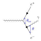
Figure 3: Photon emission from an $e^{+}e^{-}$ pair with opening angle $\theta_{ee}$. Both angles are taken to be small: $\theta,\theta_{ee}\ll 1$.

The four-momenta can be written as:

$$e^{-}~{}\text{before emission:}~{}p_{e^{*}} = (E_{e^{*}},p,\mathbf{0})\;,$$ (56)

$$\text{emitted photon:}~{}p_{\gamma} = (E_{\gamma},zp,\mathbf{k}_{T})\;,$$

$$e^{-}~{}\text{after emission:}~{}p_{e^{*}} = (E_{e},(1-z)p,-\mathbf{k}_{T})\;,$$

where $z$ is the momentum fraction of the emitted photon and $\mathbf{k}_{T}$ its transverse momentum. The energies squared are then given by (neglecting the electron mass):

$$E_{\gamma}^{2} = (zp)^{2}+\mathbf{k}_{T}^{2}\;,$$ (57)

$$E_{e*}^{2} = p^{2}\;,$$

$$E_{e}^{2} = (1-z)^{2}p^{2}+\mathbf{k}_{T}^{2}\;.$$

The energy “imbalance” at the vertex due to the emission of the photon (i.e. the “virtuality” of the electron before emission, $e^{*}$) is then:

$$\Delta E = E_{e*}+E_{\gamma}-E_{e}$$

$$= \sqrt{(zp)^{2}+\mathbf{k}_{T}^{2}}+\sqrt{(1-z)^{2}p^{2}+\mathbf{k}_{T}^{2}}-p\;,$$

which, after expansion for small transverse momentum, $|\mathbf{k}_{T}|\ll zp,(1-z)p$, becomes:

$$\Delta E\approx zp\left(1+\frac{1}{2}\frac{\mathbf{k}_{T}^{2}}{z^{2}p^{2}}\right)+(1-z)p\left(1+\frac{1}{2}\frac{\mathbf{k}_{T}^{2}}{p^{2}(1-z)^{2}}\right)-p\;,$$ (59)

which leads to:

$$\Delta E\approx\frac{1}{2}\frac{\mathbf{k}_{T}^{2}}{p}\frac{1}{z(1-z)}\;.$$ (60)

For soft emissions, $z(1-z)\sim z$ and so:

$$\Delta E\sim\frac{\mathbf{k}_{T}^{2}}{zp}\;.$$ (61)

By considering the right-angle triangle formed by the outgoing electron and the emitted photon ($\sim zp$ at an angle $\theta$), we also have: $|\mathbf{k}_{T}|\approx zp\sin\theta\approx zp\theta$ and so we are left with:

$$\Delta E\sim zp\theta^{2}.$$ (62)

Due to the uncertainty principle, the time available for photon emission is $\Delta t\sim 1/\Delta E$. During this time, the transverse separation of the $e^{+}e^{-}$ pair will become: $\Delta b\sim\theta_{ee}\Delta t$. In order for there to be a non-negligible probability of photon emisison, the photon must be able to “resolve” this separation. This will be the case if $\Delta b>\lambda/\theta$, with $\lambda$ the photon wavelength, with $\lambda\sim 1/E_{\gamma}\sim 1/(zp)$. This leads to the condition $\Delta b>1/(zp\theta)$. Substituting for $\Delta b$, we obtain:

$$\frac{\theta_{ee}}{zp\theta^{2}}>\frac{1}{zp\theta}\Rightarrow\theta_{ee}>\theta\;.$$ (63)

Photons emitted at angles $\theta>\theta_{ee}$ cannot resolve the individual $e^{+}$ and $e^{-}$ charges, i.e. they only see the net zero charge of the system. This implies that soft photon emission is suppressed at angles $\theta>\theta_{ee}$. The heuristic arguments presented thus far can be easily generalized to QCD emissions.

2.6 Remarks

The present treatment has neglected several important aspects of the parton shower, and is merely aiming to provide an introduction to its fundamental aspects. For instance, we have only been discussing ‘final-state’ emissions, i.e. radiation off outgoing particles. Initial-state radiation, e.g. from incoming quarks and gluons at the Large Hadron Collider, requires evolution ‘backwards’ to the parton density functions that describe the colliding hadrons.

Another important issue that we have not discussed is that of momentum conservation following emissions. Momentum conservation can be implemented, e.g. globally, at the end of the evolution. We will discuss this approach when outlining the details of the implementation in section 3. In a class of parton showers known as ‘dipole’ showers, the recoil is instead local and is ‘taken’ by ‘spectator’ particles.

There are also other important issues that remain:

• Hadronization: What happens below the cutoff scale?

• The treatment of multi-parton interactions and the “underlying event”.

• Matching and merging the parton shower to fixed-order matrix elements.

• Limitations of the parton shower approximation: leading color, logarithmic accuracy, etc..

3 A Toy Parton Shower

3.1 Implementation Specifics

The aim of the Pyresias toy parton shower is to simulate multiple gluon emissions from an outgoing quark (or anti-quark) line:

This treatment takes into account the collinear enhancements, and the soft wide-angle emissions are treated via angular ordering (i.e. coherent branching). We perform the branchings in a frame of reference where the parent quark is moving along the $z$ direction, and then rotate (see appendix B) all the reconstructed momenta into the appropriate direction. Therefore, the parton shower is only valid for lepton collisions, or particle decays, in the center-of-mass frame.

For coherent branching, the corresponding evolution variable is Ellis:1996mzs : $\tilde{t}=E^{2}\zeta$, for a parton of energy $E$, where $\zeta=\frac{p_{b}.p_{c}}{E_{b}E_{c}}\simeq 1-\cos\theta$ in a branching $a\rightarrow bc$. When using this variable, we have to remember that the angular ordering condition in the branching translates to:

$$\tilde{t}_{b}<z^{2}\tilde{t}\;,\qquad\tilde{t}_{c}<(1-z)^{2}\tilde{t}\;.$$ (64)

This implies, e.g. in $q\rightarrow qg$, the outgoing quark and gluon values of the evolution variable $\tilde{t}$ have to be set to the above values, respectively. Moreover, the angular ordering condition on $\zeta$ leads to:

$$z_{+}=1-\sqrt{\frac{\tilde{t}_{0}}{\tilde{t}}}\;;~{}z_{-}=\sqrt{\frac{\tilde{t}_{0}}{\tilde{t}}}\;,$$ (65)

and the cutoff on the emission scale is Ellis:1996mzs $\tilde{t}_{c}=4\tilde{t}_{0}$. Then, to obtain the kinematics from $\tilde{t}$ and $z$, for each branching:

• the virtual mass squared of $a$ in $a\rightarrow bc$ is given by $t=z(1-z)\tilde{t}$,

• and the transverse momentum squared of the branching is given by: $p_{T}^{2}=z^{2}(1-z)^{2}\tilde{t}$.

The strong coupling constant is evaluated at $Q^{2}=p_{T}^{2}$, as this captures some of the next-to-leading order behavior. The $\alpha_{S}$ values are calculated at next-to-leading order following hocheprestel ; Seymour:2024fmq . Finally, the overestimate for the $q\rightarrow qg$ splitting function is given by:

$$\hat{P}(z)=C_{F}\frac{2}{1-z}\;,$$ (66)

which satisfies $\hat{P}(z)>P(z)\forall z$. The overestimate for $\alpha_{S}$ is taken as the value of $\alpha_{S}$ at the cutoff scale.

We refer the reader to the JupyterLab notebook pyresias_nb.ipynb for further details of the implementation, as well as a detailed description of the parton shower via the Sudakov veto algorithm. The Python code pyresias_test.py is a script version of the same code, that also writes out the set of plots for the fundamental reconstruction variables.

3.2 Global Energy-Momentum Conservation

We wish to preserve the total energy of the system in the center-of-mass frame of the hard collision. If the momenta of the parent partons before before the evolution are: $p_{J}=(\mathbf{p}_{J},\sqrt{\mathbf{p}_{J}^{2}+m_{J}^{2}})$ in this frame, then they satisfy:

$$\sum_{j=1}^{n}\sqrt{\mathbf{p}_{J}^{2}+m_{J}^{2}}=\sqrt{s}\;,$$ (67)

and the sum of the spatial momenta is zero: $\sum_{j=1}^{n}\mathbf{p}_{J}=\mathbf{0}$. The jet parents have momenta $q_{J}=\left(\mathbf{q}_{J},\sqrt{\mathbf{q}_{J}^{2}+q_{J}^{2}}\right)$ after the parton shower. We need to restore momentum conservation in a way that disturbs the internal structure of the jets as little as possible. This is achieved by first rotating the outgoing jet along the original jet direction, and then boosting it along its axis such that the momenta are rescaled by a common factor $k$, determined by:

$$\sum_{j=1}^{n}\sqrt{k^{2}\mathbf{p}_{J}^{2}+q_{J}^{2}}=\sqrt{s}\;.$$ (68)

This equation can be solved analytically for 2 jets, or numerically in general, e.g. via Newton-Raphson root finding. The rotations and boosts need to be applied to each of the jets in the center-of-mass of the collisions. Schematically:

$$q_{J}=\left(\mathbf{q}_{J},\sqrt{\mathbf{q}_{J}^{2}+q_{J}^{2}}\right)\xrightarrow{rot.+boost}q_{J}^{\prime}=\left(k\mathbf{p}_{J},\sqrt{k^{2}\mathbf{p}_{J}^{2}+q_{J}^{2}}\right)\;.$$ (69)

See appendix B for details on the rotations. The Python code pyresias.py implements this reconstruction approach for the case of $e^{+}e^{-}\rightarrow q\bar{q}$.

3.3 Results

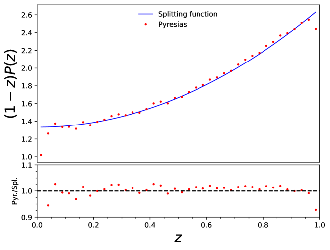
Figure 4: The distribution of the momentum fraction variable $z$ times $1-z$, compared to the analytical expression for the splitting function times $1-z$, i.e. $(1-z)P(z)$. The normalization was chosen to replicate that of the analytical splitting function, which yields $(1-z)P(z)=CF$ at $z=0$. The parton shower was run from $Q=1000$ GeV down to $Q_{c}=1$ GeV, and the scale of $\alpha_{S}$ was fixed to $Q/2$.

To verify that the splitting function is indeed reproduced in the parton shower, we ran the parton shower from $Q=1000$ GeV down to $Q_{c}=1$ GeV. The scale of $\alpha_{S}$ was fixed to $Q/2$. The result is shown in fig. 4, where the distribution of the momentum fraction variable $z$ times $1-z$, is compared to the analytical expression for the splitting function times $1-z$, i.e. $(1-z)P(z)$. The normalization was chosen to replicate that of the analytical splitting function, which yields $(1-z)P(z)=C_{F}$ at $z=0$. It is evident that the distribution of $z$ is reproduced by the parton shower algorithm within Pyresias, barring minor numerical effects near the $z=0$ and $z=1$ edges.

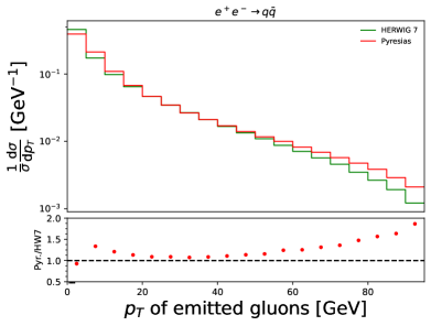
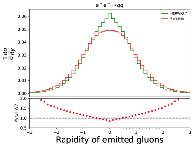
Figure 5: Comparisons between HERWIG 7 and Pyresias of the distributions of transverse momentum and rapidity of the emitted gluons generated in the showered $e^{+}e^{-}\rightarrow q\bar{q}$ process.

We then proceed to compare the Pyresias parton shower to an equivalent treatment in HERWIG 7 general-purpose Monte Carlo event generator Bahr:2008pv ; Bellm:2017bvx ; Gieseke:2011na ; Arnold:2012fq ; Bellm:2013hwb ; Bellm:2019zci ; Bewick:2023tfi , where we have switched off all splittings apart from $q\rightarrow qg$, as well as the effects of hadronization and any initial-state photon radiation. We have generated parton-level events in MadGraph5_aMCNLO Alwall:2011uj for the process $e^{+}e^{-}\rightarrow q\bar{q}$, at a center-of-mass energy of $206$ GeV, excluding the production of bottom quarks. These formed the input of both Pyresias and HERWIG 7, via the Les Houches-Accord Event File format (LHE). In fig. 5 we show comparisons of the distributions of transverse momentum and rapidity of the emitted gluons only. The agreement is reasonable, given that the calculations for $\alpha_{S}$ as well as the evolution variable are different between the two treatments.

4 Conclusions

Parton showers form an essential ingredient in the Monte Carlo simulation of collider events, and beyond. Through a parton shower, collinear emissions, including soft and collinear, can be treated via Monte Carlo, through splitting functions. Large-angle soft emissions exhibit color-coherence, and can be treated via angular ordering. In this article, we have motivated the parton shower algorithm via the Sudakov form factor, by considering multiple gluon emissions in an $e^{+}e^{-}$ collision that generates a quark-anti-quark pair. We have presented the Sudakov veto algorithm, used to implement the treatment of QCD radiation in such a formalism. We have also briefly discussed additional aspects of the event generation that interface to the parton shower, in order to obtain a full simulation of collider events. We then discussed some specific aspects of the implementation presented here in the form of a tutorial, aimed to introduce the basic concepts. The associated code produced is able to generate a parton shower consisting of the radiation of gluons from quark lines, with reasonable agreement to the widely-used HERWIG 7 general purpose event generator.

Appendix A Proof of the Sudakov Veto Algorithm

To prove the Sudakov veto algorithm, described in section 2.4, consider the total probability of not having an emission in $(t_{0},t_{\mathrm{max}})$, after rejecting (i.e. vetoing) any number of emissions:

$$\bar{P}_{\mathrm{tot}}=\sum_{n=0}^{\infty}\bar{P}_{n}\;,$$ (70)

where $\bar{P}_{n}$ is the probability that we have rejected $n$ intermediate trial values of the evolution variable via the Sudakov veto algorithm (SVA). We then have, for no vetoed emissions ($n=0$):

$$\bar{P}_{0}=\hat{\Delta}(t_{0},t_{\mathrm{max}})\;,$$ (71)

where is $\hat{\Delta}(t_{0},t_{\mathrm{max}})$ is the underestimate of the true Sudakov factor, defined by eq. 39. The probability that we have rejected exactly one emission is:

$$\bar{P}_{1}=\int_{t_{0}}^{t_{\mathrm{max}}}\mathrm{d}t\hat{\Gamma}(t)\hat{\Delta}(t,t_{\mathrm{max}})\left[1-\frac{\Gamma(t)}{\hat{\Gamma(t)}}\right]\hat{\Delta}(t_{0},t)\;,$$ (72)

where we have integrated over all trial scales $t$ that have been rejected, and the factor $\hat{\Gamma}(t)\hat{\Delta}(t,t_{\mathrm{max}})$ represents the probability of a first trial emission occurring at $t$, the factor $\left[1-\frac{\Gamma(t)}{\hat{\Gamma(t)}}\right]$ represents the probability that we have rejected it, and $\hat{\Delta}(t_{0},t)$ ensures that there are no further emissions between $t$ and $t_{0}$.

By using the property of the Sudakov form factor that $\hat{\Delta}(t_{0},t)\hat{\Delta}(t,t_{\mathrm{max}})=\hat{\Delta}(t_{0},t_{\mathrm{max}})$, we can then write:

$$\bar{P}_{1}=\hat{\Delta}(t_{0},t_{\mathrm{max}})\int_{t_{0}}^{t_{\mathrm{max}}}\mathrm{d}t\left[\hat{\Gamma}(t)-\Gamma(t)\right]\;.$$ (73)

This procedure can be extended to $n=2$ vetoed emissions via the SVA:

$$\bar{P}_{2}=\int_{t_{0}}^{t_{\mathrm{max}}}\mathrm{d}t_{1}\hat{\Gamma}(t_{1})\hat{\Delta}(t_{1},t_{\mathrm{max}})\left[1-\frac{\Gamma(t_{1})}{\hat{\Gamma(t_{1})}}\right]\int_{t_{0}}^{t_{1}}\mathrm{d}t_{2}\hat{\Gamma}(t_{2})\hat{\Delta}(t_{1},t_{2})\left[1-\frac{\Gamma(t_{2})}{\hat{\Gamma(t_{2})}}\right]\hat{\Delta}(t_{0},t_{2})\;,$$ (74)

where $t_{1}$ now represents the scale of the first rejected emission, with probability $\hat{\Gamma}(t_{1})\hat{\Delta}(t_{1},t_{\mathrm{max}})$, and rejected with probability $\left[1-\frac{\Gamma(t_{1})}{\hat{\Gamma(t_{1})}}\right]$, $t_{2}<t_{1}$ represents the scale of the second emission, with probability $\hat{\Gamma}(t_{2})\hat{\Delta}(t_{1},t_{2})$, and $\hat{\Delta}(t_{0},t_{2})$ is the probability that there are no further emissions between $t_{2}$ and $t_{0}$. Using the property of the Sudakov form factor as we did for $n=1$, we then find that:

$$\bar{P}_{2}=\hat{\Delta}(t_{0},t_{\mathrm{max}})\int_{t_{0}}^{t_{\mathrm{max}}}\left[\hat{\Gamma}(t_{1})-\Gamma(t_{1})\right]\int_{t_{0}}^{t_{\mathrm{max}}}\left[\hat{\Gamma}(t_{2})-\Gamma(t_{2})\right]\;,$$ (75)

where $t_{0}<t_{2}<t_{1}<t_{\mathrm{max}}$, or, equivalently:

$$\bar{P}_{2}=\hat{\Delta}(t_{0},t_{\mathrm{max}})\frac{1}{2!}\left(\int_{t_{0}}^{t_{\mathrm{max}}}\left[\hat{\Gamma}(t)-\Gamma(t)\right]\right)^{2}\;,$$ (76)

Therefore, for $n$ vetoed emissions:

$$\bar{P}_{n}=\hat{\Delta}(t_{0},t_{\mathrm{max}})\frac{1}{n!}\left(\int_{t_{0}}^{t_{\mathrm{max}}}\left[\hat{\Gamma}(t)-\Gamma(t)\right]\right)^{n}\;,$$ (77)

and hence the total probability of not having an emission in $(t_{0},t_{\mathrm{max}})$ turns into:

$$\bar{P}_{\mathrm{tot}}=\sum_{n=0}^{\infty}\bar{P}_{n}=\hat{\Delta}(t_{0},t_{\mathrm{max}})\sum_{n=0}^{\infty}\frac{1}{n!}\left(\int_{t_{0}}^{t_{\mathrm{max}}}\left[\hat{\Gamma}(t)-\Gamma(t)\right]\right)^{n}\;,$$ (78)

or:

$$\bar{P}_{\mathrm{tot}}=\sum_{n=0}^{\infty}\bar{P}_{n}=\hat{\Delta}(t_{0},t_{\mathrm{max}})\exp\left\{\left[\hat{\Gamma}(t)-\Gamma(t)\right]\right\}\;.$$ (79)

Comparing with eq. 39, we can now see that the first term in the exponential cancels out the Sudakov form factor underestimate, therefore yielding:

$$\bar{P}_{\mathrm{tot}}=\Delta(t_{0},t_{\mathrm{max}})\;,$$ (80)

i.e. the original Sudakov form factor!

We have therefore demonstrated that via the SVA one recovers the correct Sudakov form factor as the probability of having no emission between $(t_{0},t_{\mathrm{max}})$, as required.

Appendix B Rotations

To rotate a 3-vector $\mathbf{a}$ on a 3-vector $\mathbf{b}$, we first construct the axis unit vector by taking their cross product: $\hat{\mathbf{k}}=\frac{\mathbf{a}\times\mathbf{b}}{|\mathbf{a}\times\mathbf{b}|}$. Then, the rotation is given by the Euler-Rodrigues’ rotation formula:

$$\mathbf{R}=\mathbf{I}+(\sin\theta)\mathbf{K}+(1-\cos\theta)\mathbf{K}^{2}\;,$$ (81)

where $\mathbf{I}$ is the identity matrix, $\theta$ is the angle between $\mathbf{a}$ and $\mathbf{b}$, and the matrix $\mathbf{K}$ takes the form:

$$\mathbf{K}=\begin{pmatrix}0&-\hat{k}_{z}&\hat{k}_{y}\\ \hat{k}_{z}&0&-\hat{k}_{x}\\ -\hat{k}_{y}&\hat{k}_{x}&0\end{pmatrix}\;,$$ (82)

and then the rotated vector $\mathbf{a}^{\prime}$ is given by $\mathbf{a}^{\prime}=\mathbf{R}\mathbf{a}$.

References

- (1) A. Papaefstathiou, “Pyresias: A Toy Parton Shower for Educational Purposes.” https://github.com/apapaefs/pyresias, 2024.
- (2) G.C. Fox and S. Wolfram, A Model for Parton Showers in QCD, Nucl. Phys. B 168 (1980) 285.
- (3) G. Marchesini and B.R. Webber, Simulation of QCD Jets Including Soft Gluon Interference, Nucl. Phys. B 238 (1984) 1.
- (4) W.T. Giele, T. Matsuura, M.H. Seymour and B.R. Webber, W boson plus multijets at hadron colliders: HERWIG parton showers versus exact matrix elements, in 1990 DPF Summer Study on High-energy Physics: Research Directions for the Decade (Snowmass 90), pp. 0137–147, 11, 1990.
- (5) B.R. Webber, Recent progress in QCD jet physics in e+e- collisions, AIP Conf. Proc. 272 (2008) 878.
- (6) A. Buckley et al., General-purpose event generators for LHC physics, Phys. Rept. 504 (2011) 145 [1101.2599].
- (7) J.M. Campbell et al., Event Generators for High-Energy Physics Experiments, in Snowmass 2021, 3, 2022 [2203.11110].
- (8) R.K. Ellis, W.J. Stirling and B.R. Webber, QCD and collider physics, vol. 8, Cambridge University Press (2, 2011), 10.1017/CBO9780511628788.
- (9) S. Gieseke, “Parton Shower Monte Carlo.” https://www.itp.kit.edu/~gieseke/uam/madrid16.pdf, 2023.
- (10) L. Lönnblad, Fooling Around with the Sudakov Veto Algorithm, Eur. Phys. J. C 73 (2013) 2350 [1211.7204].
- (11) M. Bahr et al., Herwig++ Physics and Manual, Eur. Phys. J. C58 (2008) 639 [0803.0883].
- (12) S. Höche, Introduction to parton-shower event generators, in Theoretical Advanced Study Institute in Elementary Particle Physics: Journeys Through the Precision Frontier: Amplitudes for Colliders, pp. 235–295, 2015, DOI [1411.4085].
- (13) S. Höche and S. Prestel, “Tutorial on Parton Showers and Matching.” https://www.slac.stanford.edu/~shoeche/mcnet16/ws/PS.pdf, 2016.
- (14) M.H. Seymour and S. Sule, An Algorithm to Parallelise Parton Showers on a GPU, 2403.08692.
- (15) R.D. Field, Applications of Perturbative QCD, vol. 77 (1989).
- (16) F. Bloch and A. Nordsieck, Note on the Radiation Field of the electron, Phys. Rev. 52 (1937) 54.
- (17) T. Kinoshita, Mass singularities of Feynman amplitudes, J. Math. Phys. 3 (1962) 650.
- (18) T.D. Lee and M. Nauenberg, Degenerate Systems and Mass Singularities, Phys. Rev. 133 (1964) B1549.
- (19) J. Bellm et al., Herwig 7.1 Release Note, 1705.06919.
- (20) S. Gieseke et al., Herwig++ 2.5 Release Note, 1102.1672.
- (21) K. Arnold et al., Herwig++ 2.6 Release Note, 1205.4902.
- (22) J. Bellm et al., Herwig++ 2.7 Release Note, 1310.6877.
- (23) J. Bellm et al., Herwig 7.2 release note, Eur. Phys. J. C 80 (2020) 452 [1912.06509].
- (24) G. Bewick et al., Herwig 7.3 Release Note, 2312.05175.
- (25) J. Alwall, M. Herquet, F. Maltoni, O. Mattelaer and T. Stelzer, MadGraph 5 : Going Beyond, JHEP 06 (2011) 128 [1106.0522].