Astrometric Detection of Ultralight Dark Matter

Abstract

Ultralight dark matter induces time-dependent perturbations in the spacetime metric, enabling its gravitational direct detection. In this work, we propose using astrometry to detect dark matter. After reviewing the calculation of the metric in the presence of scalar dark matter, we study the influence of the perturbations on the apparent motion of astrophysical bodies. We apply our results to angular position measurements of quasars, whose vast distances from Earth present an opportunity to discover dark matter with a mass as low as $10^{-33}\,\mathrm{eV}$. We explore the prospects of very long baseline interferometry and optical astrometric survey measurements for detecting ultralight relics, finding that for the smallest masses, current astrometric surveys can detect dark matter moving locally with a velocity of $10^{-3}$ with energy density as low as $3\times 10^{-11}~{}{\rm GeV}/{\rm cm}^{3}$.

Introduction. To date, all successful attempts to infer the presence of dark matter have relied solely on its gravitational interactions with the visible sector. What if dark matter only interacts gravitationally? It was recently demonstrated that, in this case, it is still possible to directly detect dark matter through time-dependent perturbations to the spacetime metric generated by its coherent oscillations Khmelnitsky and Rubakov (2014). These perturbations cause a gravitational redshift that can be measured by analyzing pulsar timing array (PTA) data, provided dark matter has a de Broglie wavelength shorter than the distance to typical millisecond pulsars, corresponding to a mass $m\gtrsim 10^{-24}~{}{\rm eV}$. Experimental searches have since been conducted by the Parkes PTA Porayko et al. (2018), the European PTA Smarra et al. (2023), and NANOGrav Afzal et al. (2023). Concurrently, there is an ongoing large-scale theory effort to understand the detection prospects of the dark matter-induced gravitational redshift using gravitational wave instruments (see, e.g., Refs. Porayko and Postnov (2014); Graham et al. (2016); Aoki and Soda (2016a, b); Blas et al. (2017); De Martino et al. (2017); Kato and Soda (2020); Nomura et al. (2020); Kaplan et al. (2022); Xia et al. (2023); Luu et al. (2024); Kim (2023); Hwang et al. (2024); Kim and Mitridate (2024); Brax et al. (2024)).

In this Letter, we propose a second method for the gravitational direct detection of dark matter: measuring the apparent angular positions of astrophysical bodies, a technique known as astrometry. Astrometry has seen significant advancements with the maturation of very long baseline interferometry (VLBI), which achieves positional uncertainties as low as 1 $\mu$as for a small number of sources, and the advent of space-based optical telescopes, which, despite having higher positional uncertainties, provide recurrent measurements of billions of sources Reid and Honma (2014); Thompson et al. (2017).

For an observer moving at a non-relativistic instantaneous velocity, ${\mathbf{v}}_{\rm o}$, with a constant acceleration, ${\bf a}_{\rm o}$, the angular position of an astrophysical source moving at ${\mathbf{v}}_{\rm s}$ at a far distance ${\mathbf{x}}_{s}$ exhibits known kinematic corrections. The apparent proper motion in an angular direction $\hat{\theta}$ is,

$$\omega_{\theta}=\left[\dot{{\mathbf{v}}}_{\rm o}-\frac{{\mathbf{v}}_{\rm o}-{\mathbf{v}}_{\rm s}}{x_{\rm s}}+{\bf a}_{\rm o}\right]\cdot\hat{\theta}\,,$$ (1)

with the terms known as classical aberration, intrinsic proper motion, and the secular aberration drift, respectively. In Eq. (1), we only present the leading term for each type of correction.

Classical aberration is sizable for every source, inducing a typical proper motion of ${\cal O}(100~{}{\rm as}/{\rm year})$ for observers orbiting the Sun, and is routinely corrected for (see, e.g., Ref. Klioner (2003)). For extragalactic sources (the focus of this work), the second term in Eq. (1) is negligible. For the Milky Way potential, the acceleration-induced proper motion is measured to be $4.80\pm 0.08~{}\mu{\rm as}/{\rm year}$ Titov et al. (2011); Gaia Collaboration et al. (2021), displaying a dipolar pattern across the sky.

Ultralight dark matter also induces an apparent angular deflection independent of the source distance. We calculate the effect in this work, finding two characteristic signals: a secular proper motion analogous to the secular aberration drift and an annual modulation analogous to the classical aberration. Importantly, the size of the effect depends on the hierarchy between the source distance and the inverse dark matter mass so that, for a large range of masses, galactic and extragalactic sources exhibit a different deflection. This provides a method to distinguish the signal from other backgrounds.

For a fixed density, the dark matter-induced angular deflection is most pronounced at the lowest dark matter masses. The cosmological distances of quasars enable the detection of dark matter with masses as low as the current Hubble constant. As such, we focus on the detection of dark matter using quasars, though most of our expressions can be applied to astrometry of any point source.

Our findings pave the way for astrometry to revolutionize the prospects of gravitational direct detection of dark matter. As we show, this method is sensitive to minuscule densities and is a powerful probe of the existence of ultralight particles.

Ultralight Scalar Dark Matter. Ultralight scalar dark matter can be modeled as a classical field, $a(t,{\mathbf{x}})$, oscillating primarily at a frequency $\Omega$ with a slowly varying phase, $\alpha(t,\mathbf{x})$,

$$a(t,\mathbf{x})=a_{0}(\mathbf{x})\cos\left(\Omega t+\alpha(t,\mathbf{x})\right)\,.$$ (2)

The velocity distribution of the field is encapsulated in the properties of $\alpha(t,{\mathbf{x}})$ (see, e.g., Refs. Foster et al. (2021); Dror et al. (2023) for further details). This phase can be decomposed as $-m{\mathbf{v}}_{a}\cdot{\mathbf{x}}+\alpha_{0}$, where ${\mathbf{v}}_{a}$ represents the field velocity relative to the cosmic frame. The offset $\alpha_{0}$ and the direction of ${\mathbf{v}}_{a}$ are randomly sampled every coherence time and coherence length of the field (both quantities determined by the dark matter velocity distribution). The momentum of the field, ${\mathbf{k}}\equiv\nabla\alpha=-m{\mathbf{v}}_{a}+\nabla\alpha_{0}$, is related to the frequency through the Klein-Gordon equation, $\left(\Box-m^{2}\right)a(t,\mathbf{x})$ (in the non-relativistic limit, $\Omega=m+k^{2}/2m$). The conditions under which the field can be accurately approximated by a fluctuating plane wave form are $k\gg\nabla a_{0}/a_{0}$ and $\Omega\gg\partial_{t}\alpha$, and we assume these conditions throughout.

Ultralight dark matter generates time-dependent perturbations in the stress-energy tensor, resulting in oscillating perturbations to the spacetime metric through Einstein’s equations Khmelnitsky and Rubakov (2014). The stress-energy tensor of a scalar field in an otherwise flat spacetime is given by:

$$\tensor{T}{{}_{\mu}{}_{\nu}}=\partial_{\mu}a\partial_{\nu}a-\tensor{\eta}{{}_{\mu}{}_{\nu}}\left(\frac{1}{2}\eta^{\sigma\rho}\partial_{\sigma}a\partial_{\rho}a+\frac{1}{2}m^{2}a^{2}\right)\,,$$ (3)

where $\eta\equiv{\rm diag}(-1,1,1,1)$. Inserting the form of $a(t,{\mathbf{x}})$ from Eq. (2) into this expression yields oscillating energy density $\rho\equiv T_{00}$ and pressure $P\equiv\frac{1}{3}T_{ii}$ terms at a frequency of $2\Omega$:

$$\rho =\frac{1}{2}a_{0}^{2}\left[m^{2}+k^{2}-k^{2}\cos\left(2(\Omega t+\alpha)\right)\right]\,,$$ (4)

$$P =\frac{1}{2}a_{0}^{2}\left[\frac{1}{3}k^{2}-\left(m^{2}+\frac{1}{3}k^{2}\right)\cos\left(2(\Omega t+\alpha)\right)\right]\,.$$ (5)

In deriving these expressions, we neglected $\nabla a_{0}$ and $\partial_{t}\alpha$ terms (see discussion above) and terms of ${\cal O}(k^{4})$. The results agree with Ref. Khmelnitsky and Rubakov (2014) at ${\cal O}(k^{0})$. Since the Einstein equations are second-order differential equations, it is useful to retain the (naively) higher-order terms. While our interest is in experiments that resolve the time oscillation, we note that, upon time-averaging, the pressure vanishes and the energy density takes the familiar form, $\rho\simeq\frac{1}{2}m^{2}a_{0}^{2}$.

The oscillatory nature of the stress-energy components generates time-dependent scalar perturbations in the spacetime metric. The scalar-vector-tensor decomposition theorem (see, e.g., Ref. Maggiore (2018)) ensures that the scalar perturbations generate scalar metric perturbations. In Newtonian gauge, the metric is characterized by two scalar functions, $\phi$ and $\psi$, such that the line element is given by,

$$ds^{2}=-(1+2\psi(t,{\bf{x}}))dt^{2}+\left(1-2\phi(t,{\bf{x}})\right)\delta_{ij}dx^{i}dx^{j}\,.$$ (6)

These gravitational potentials decompose into time-independent and time-dependent contributions with frequency $2\Omega$ Khmelnitsky and Rubakov (2014):

$$\psi =\psi_{0}+\psi_{c}\cos\left(2(\Omega t+\alpha)\right)+\psi_{s}\sin\left(2(\Omega t+\alpha)\right),$$ (7)

$$\phi =\phi_{0}+\phi_{c}\cos\left(2(\Omega t+\alpha)\right)+\phi_{s}\sin\left(2(\Omega t+\alpha)\right)\,,$$ (8)

where the coefficients $\psi_{0},\psi_{c},\psi_{s},\phi_{0},\phi_{c},\phi_{s}$ depend only on ${\mathbf{x}}$. Combining Einstein equations in Newtonian gauge,

$$\nabla^{2}\phi=4\pi G\rho\,,\quad\ddot{\phi}+\frac{1}{3}\nabla^{2}\left(\psi-\phi\right)=4\pi GP\,,$$ (9)

with Eqs. (4) and (5), and separating the time-dependent and time-independent contributions, we find that the gravitational potentials are:

$$\psi_{c}(\mathbf{x})=-\phi_{c}({\mathbf{x}})=-\frac{1}{2}\pi Ga_{0}^{2}(\mathbf{x})\,,\phi_{s}=\psi_{s}=0\,,$$ (10)

where $G$ denotes the gravitational constant. $\phi_{0}(\mathbf{x})$ and $\psi_{0}(\mathbf{x})$ describe the static gravitational potential and are indistinguishable from those of cold dark matter, which we neglect in our analysis. In the following analysis, we focus on dark matter by replacing $\psi$ with $-\phi$.

Astrometric Deflection of Dark Matter. The dark matter metric perturbations cause fluctuations in the apparent positions of distant astrophysical sources. We now derive this effect working to first order in the size of the perturbation, assuming they are superimposed on a flat Minkowski background. Although our results can be readily generalized to a Friedmann-Robertson-Walker (FRW) metric via a conformal transformation Book and Flanagan (2011), the results remain unchanged in the limit when $\Omega$ is large compared to the inverse source distance. For quasars (typically at cosmological distances), this holds for all masses well above the Hubble scale today.

In the absence of metric perturbations, light emitted from a source with frequency $\omega_{0}$ traveling in the $-\hat{\bf n}$ direction has the following position and momentum four-vectors:

$$x^{\mu}(\lambda) =\left(\omega_{0}\lambda+t_{{\rm o}},-\omega_{0}\lambda\hat{\bf{n}}\right)\,,$$ (11)

$$p^{\mu}(\lambda) =\omega_{0}\left(1,-\hat{\bf{n}}\right)\,.$$ (12)

Here, $\lambda$ is the affine parameter, with a value of $\lambda_{{\rm s}}\equiv-\left|{\mathbf{x}}_{{\rm s}}\right|/\omega_{0}$ corresponding to photon emission and $0$ at photon arrival, while $t_{{\rm o}}$ represents the time of photon observation. We choose the observer to be at the origin upon observation, moving at velocity ${\mathbf{v}}_{{\rm o}}$, and the source at rest (our results are insensitive to this assumption), with position four-vectors $x^{\mu}_{\rm o}(t)=(t,{\mathbf{0}})$, $x_{\rm s}^{\mu}(t)=(t,{\bf x}_{\rm s})$. Our goal is to solve for the angular deflection in the limit of small velocities. Thus, we will only retain terms of ${\cal O}(v_{\rm o})$. For example, we take the four-velocity of the observer as $u_{\rm o}^{\mu}=(1,{\mathbf{v}}_{\rm o})$.

In preparation for the perturbed calculation, we introduce a coordinate system for the observer in the absence of metric perturbations, $(e^{\mu}_{\hat{0}},e^{\mu}_{\hat{1}},e^{\mu}_{\hat{2}},e^{\mu}_{\hat{3}})$. We set the basis vector $e_{\hat{0}}^{\mu}$ equal to the observer’s four-velocity. Requiring the basis be orthogonal ($\eta_{\mu\nu}e_{\hat{\alpha}}^{\mu}e_{\hat{\beta}}^{\nu}=\eta_{\hat{\alpha}\hat{\beta}}$) implies $e^{i}_{\hat{j}}=\delta^{i}_{\hat{j}}$ and $e_{\hat{a}}^{0}=v_{\hat{a}}$ (up to velocity-squared corrections). Here and throughout, the hatted indices denote the observer frame and the unhatted indices denote the coordinate frame.

The apparent four-momentum of the source in the observer frame is given by $p_{\hat{\alpha}}=\eta_{\mu\nu}p^{\mu}e^{\nu}_{\hat{\alpha}}$, which gives an observed photon frequency and 3-momentum,

$$p_{\hat{0}}=-\omega_{0}(1+\hat{\bf n}\cdot{\mathbf{v}}_{\rm o})\,,\,p_{\hat{a}}=-\omega_{0}(\hat{\bf n}+{\mathbf{v}}_{\rm o})_{\hat{a}}\,.$$ (13)

At first order in the perturbations, there are three gauge-dependent effects: the photon worldline and momentum perturbations ($\delta x^{\mu}(\lambda)$ and $\delta p^{\mu}(\lambda)$), the source and the observer worldline perturbations ($\delta x_{\rm s}(\lambda)$ and $\delta x_{{\rm o}}(\lambda)$), and the frame deformation in the local proper reference frame of the observer, $\delta e_{\hat{\alpha}}^{\mu}(\lambda)$. The trajectory of the photon in the presence of perturbations is depicted in Fig. 1. To find the deflection of the source, we calculate its four-momentum in the observer frame,

$$p_{\hat{\alpha}}+\delta p_{\hat{\alpha}}=(\eta_{\mu\nu}+h_{\mu\nu}(0))(p^{\mu}+\delta p^{\mu}(0))(e^{\nu}_{\hat{\alpha}}+\delta e^{\nu}_{\hat{\alpha}}(0))\,.$$ (14)

The apparent direction of the source, $\hat{n}_{\hat{i}}+\delta\hat{n}_{\hat{i}}=(p_{\hat{i}}+\delta p_{\hat{i}}(0))/(p_{\hat{0}}+\delta p_{\hat{0}}(0))$, is gauge-independent. Its calculation requires expressions for $\delta p^{\mu}(0)$ and $\delta e^{\mu}_{\hat{\alpha}}(0)$.

Figure 1: Depiction of the influence of dark matter on astrometry: In a general gauge, dark matter affects the photon path, the locations of the source and observer, and the observer’s reference frame.

We begin by calculating the first-order correction to the photon four-momentum using the geodesic equation,

$$\frac{d\delta p^{\mu}}{d\lambda}=-\Gamma^{\mu}_{\nu\rho}(\lambda)p^{\nu}p^{\rho}\,,$$ (15)

where it is understood that the Christoffel symbols are evaluated along the trajectory of the photon at zeroth order. The time and space component differential equations are analogous in the limit that $\psi=-\phi$. Their solutions are,

$$\delta p^{0}(\lambda) =\delta p^{0}(\lambda_{\rm s})+2\omega_{0}\left[\phi(\lambda)-\phi(\lambda_{{\rm s}})\right]\,,$$ (16)

$$\delta{\mathbf{p}}(\lambda) =\delta{\mathbf{p}}(\lambda_{{\rm s}})-2\omega_{0}\left[\phi(\lambda)-\phi(\lambda_{{\rm s}})\right]\hat{\bf n}\,.$$ (17)

To calculate the observed photon four-momentum, we must determine the integration constants, $\delta p^{\mu}(\lambda_{\rm s})$. We will extract these by imposing a set of boundary conditions, two of which relate the photon worldline to the observer and source worldlines. To impose these conditions, we need the expression for the photon worldline perturbation, found by integrating the momentum equation,

$$\delta{\mathbf{x}}(\lambda)=\delta{\mathbf{x}}(\lambda_{{\rm s}})+(\lambda-\lambda_{\rm s})\delta{\mathbf{p}}(\lambda_{{\rm s}})-2\omega_{0}\hat{\bf n}\int_{\lambda_{\rm s}}^{\lambda}\phi(\lambda^{\prime})-\phi(\lambda_{{\rm s}})d\lambda^{\prime}\,.$$ (18)

We calculate the source and observer location perturbations using their geodesic equations, which we parameterize using the photon’s affine parameter,

$$\frac{1}{\omega_{0}^{2}}\frac{d^{2}\delta x^{\mu}_{\rm s}}{d\lambda^{2}} =\frac{1}{\omega_{0}}\frac{d\delta u^{\mu}_{\rm s}}{d\lambda}=-\Gamma^{\mu}_{\nu\rho}(\lambda)u^{\nu}_{\rm s}u^{\rho}_{\rm s}\,,$$ (19)

$$\frac{1}{\omega_{0}^{2}}\frac{d^{2}\delta x^{\mu}_{\rm o}}{d\lambda^{2}} =\frac{1}{\omega_{0}}\frac{d\delta u^{\mu}_{\rm o}}{d\lambda}=-\Gamma^{\mu}_{\nu\rho}(\lambda)u^{\nu}_{\rm o}u^{\rho}_{\rm o}\,,$$ (20)

where the Christoffel symbols are evaluated along the zeroth order trajectory of the source and observer. Solving the differential equation with the metric given in Eq. (6) and dropping unobservable constants yields the spatial perturbations,

$$\delta{\mathbf{u}}_{\rm o}(\lambda)=\omega_{0}\int^{\lambda}_{\lambda_{\rm ref}}2{\mathbf{v}}_{{\rm o}}\dot{\phi}(t(\lambda^{\prime}),{\mathbf{0}})+\nabla\phi(t(\lambda^{\prime}),{\mathbf{0}})d\lambda^{\prime}\,,$$ (21)

$$\delta{\mathbf{u}}_{\rm s}(\lambda)=\omega_{0}\int^{\lambda}_{\lambda_{\rm ref}}\nabla\phi(t(\lambda^{\prime}),{\mathbf{x}}_{\rm s})d\lambda^{\prime}\,.$$ (22)

The lower bound on the integral is taken at an unphysical reference point, $\lambda_{\rm ref}$, and we have dropped an unmeasurable integration constant. Note that the integrands are implicitly functions of $\lambda$ from the zero-order relation, $t(\lambda)=\omega_{0}\lambda+t_{{\rm o}}$. Additionally, we evaluate the perturbations of the observer at the origin, neglecting the observer displacement due to their zeroth-order velocity. Including this displacement throughout introduces corrections suppressed by the distance to the source and we have checked that they do not meaningfully influence our final result. Integrating the geodesic equations once more yields expressions for the deflection of the observer and source positions:

$$\delta{\mathbf{x}}_{{\rm o}} =\omega_{0}\int_{\lambda_{{\rm ref}}}^{\lambda}d\lambda^{\prime}\delta{\mathbf{u}}_{\rm o}(\lambda^{\prime})\,,~{}\delta{\mathbf{x}}_{{\rm s}}=\omega_{0}\int_{\lambda_{{\rm ref}}}^{\lambda}d\lambda^{\prime}\delta{\mathbf{u}}_{\rm s}(\lambda^{\prime})\,.$$ (23)

Finally, we need the expression for the zeroth component of the four-velocities. For a moving observer in the non-relativistic limit, $\delta u^{0}_{{\rm o}}(\lambda)=\phi(t(\lambda),{\mathbf{0}})+\delta{\mathbf{u}}_{\rm o}\cdot{\mathbf{v}}_{\rm o}$, while for a static source, $\delta u^{0}_{{\rm s}}(\lambda)=\phi(t(\lambda),{\mathbf{x}}_{\rm s})$.

We are now ready to calculate the four integration constants $\delta p^{\mu}(\lambda_{{\rm s}})$ by imposing four boundary conditions.

Photon geodesic is null.

The null geodesic condition is $(\eta_{\mu\nu}+h_{\mu\nu}(\lambda))(p^{\mu}+\delta p^{\mu}(\lambda))(p^{\nu}+\delta p^{\nu}(\lambda))=0$ for any value of $\lambda$. Evaluating this constraint at $\lambda=\lambda_{\rm s}$, leads to:

$$\hat{\bf n}\cdot\delta{\mathbf{p}}(\lambda_{\rm s})=-\delta p^{0}(\lambda_{\rm s})\,.$$ (24)

Photon frequency at emission is $\omega_{0}$.

The emitted frequency of the photon is given in terms of the metric, photon four-momentum, and the source velocity at $\lambda=\lambda_{\rm s}$:

$$\omega_{0}=-(\eta_{\mu\nu}+h_{\mu\nu}(\lambda_{\rm s}))(p^{\mu}+\delta p^{\mu}(\lambda_{\rm s}))(u_{\rm s}^{\nu}+\delta u_{\rm s}^{\nu}(\lambda_{\rm s}))\,.$$ (25)

This simplifies to:

$$\delta p^{0}(\lambda_{\rm s})=\omega_{0}\left[\phi(\lambda_{\rm s})+\hat{\bf n}\cdot\delta{\mathbf{u}}_{{\rm s}}(\lambda_{\rm s})\right]\,.$$ (26)

Photon and observer worldlines intersect.

The perturbed photon path must intersect with the observer, which generically pushes the observed affine parameter away from $0$. However, we can set $\lambda$ at observation to $0$ even at first order using the reparametrization symmetry of the affine parameter, $\lambda\rightarrow a\lambda+b$. Then, at first order, requiring the photon intersect the observer sets $\delta{\mathbf{x}}(0)=\delta{\mathbf{x}}_{\rm o}(0)$. Equivalently, using Eq. (18),

$$\delta{\mathbf{x}}(\lambda_{{\rm s}})=\delta{\mathbf{x}}_{\rm o}(0)+\lambda_{\rm s}\delta{\mathbf{p}}(\lambda_{{\rm s}})+2\omega_{0}\hat{\bf n}\int_{\lambda_{\rm s}}^{0}\phi(\lambda^{\prime})-\phi(\lambda_{{\rm s}})d\lambda^{\prime}\,.$$ (27)

This fixes $\delta{\mathbf{x}}(\lambda_{{\rm s}})$; a quantity we require to apply the final boundary condition.

Photon and source worldlines intersect.

The perturbed photon path must intersect with the source. This requires a correction to the affine parameter at emission $\delta\lambda_{{\rm s}}$, which cannot be redefined away. Matching the source position to the photon location implies,

$${\mathbf{x}}_{\rm s}(\lambda_{\rm s}+\delta\lambda_{\rm s})={\mathbf{x}}(\lambda_{{\rm s}}+\delta\lambda_{{\rm s}})+\delta{\mathbf{x}}(\lambda_{{\rm s}})\,.$$ (28)

Equating the first-order correction terms,

$$\delta{\mathbf{x}}_{\rm s}(\lambda_{\rm s})=-\delta\lambda_{\rm s}\omega_{0}\hat{\bf n}+\delta{\mathbf{x}}(\lambda_{{\rm s}})\,,$$ (29)

where $\delta{\mathbf{x}}(\lambda_{\rm s})$ is fixed from Eq. (27). Since we already have the component of $\delta{\mathbf{p}}(\lambda_{\rm s})$ parallel to $\hat{\bf n}$ from Eqs. (24) and (26), we just need the perpendicular component. To this end, we take the cross product of Eq. (29) with $\hat{\bf n}$:

$$\hat{\bf n}\times\delta{\mathbf{p}}(\lambda_{{\rm s}})=\frac{1}{\lambda_{\rm s}}\hat{\bf n}\times\left[\delta{\mathbf{x}}_{\rm s}(\lambda_{\rm s})-\delta{\mathbf{x}}_{\rm o}(0)\right]\,.$$ (30)

Combining the results for the parallel and perpendicular components, the spatial integration constants are:

$$\textasciiacute\delta{\mathbf{p}}(\lambda_{\rm s}) =-\omega_{0}\hat{\bf n}\left[\phi(\lambda_{\rm s})+\hat{\bf n}\cdot\delta{\mathbf{u}}_{{\rm s}}(\lambda_{\rm s})\right]$$

$$\qquad-\frac{1}{\lambda_{\rm s}}\hat{\bf n}\times\left[\hat{\bf n}\times\left[\delta{\mathbf{x}}_{\rm s}(\lambda_{\rm s})-\delta{\mathbf{x}}_{\rm o}(0)\right]\right]\,.$$ (31)

Eqs. (26) and (31) can now be input into Eq. (17) to give the photon four-momentum at $\lambda=0$ in the coordinate frame.

Next, we compute the deformation of the observer reference frame, fixing $\delta e^{\mu}_{\hat{0}}=\delta u^{\mu}_{{\rm o}}$. We determine the perturbation to the spatial basis vectors using the parallel transport equation at first order in the perturbation size and observer velocity,

$$\frac{1}{\omega_{0}}\frac{d\delta e^{\nu}_{\hat{a}}}{d\lambda}=-\left[\Gamma^{\nu}_{0\alpha}e^{\alpha}_{\hat{\alpha}}+v^{j}_{\rm o}\Gamma_{j\rho}^{\nu}e_{\hat{\alpha}}^{\rho}\right]\,,$$ (32)

where the Christoffel symbols are evaluated along the observer worldline. Solving the equations gives,

$$\delta e_{\hat{a}}^{i} =\phi(t,{\mathbf{0}})\delta_{\hat{a}}^{i}\,,$$ (33)

$$\delta e^{0}_{\hat{a}} =\omega_{0}\int_{\lambda_{\rm ref}}^{\lambda}2v_{{\rm o},\hat{a}}\dot{\phi}(t^{\prime}(\lambda),{\mathbf{0}})+\partial_{\hat{a}}\phi(t^{\prime}(\lambda),{\mathbf{0}})d\lambda^{\prime}\,,$$ (34)

up to omitted integration constants which are time-independent and unobservable.

We now have all the ingredients to calculate the observed photon four-momentum using Eq. (14). We are interested in angular deflection, so terms proportional to $\hat{\bf n}$ drop out. The deflection in the $\hat{\theta}$ direction is given by,

$$\delta{\hat{\mathbf{n}}}\cdot\hat{\theta} =\frac{1}{D}\bigg{[}\delta e^{0}_{\hat{a}}-\hat{n}^{j}\delta e^{j}_{\hat{0}}v_{{\rm o},\hat{a}}-\delta e^{0}_{\hat{0}}v_{{\rm o},\hat{a}}-\frac{\delta p^{j}(0)\delta_{\hat{a}}^{j}}{\omega_{0}}\bigg{]}\hat{\theta}^{\hat{a}},$$ (35)

where $D\equiv 1+\hat{\bf n}\cdot{\mathbf{v}}_{\rm o}$. Our primary interest is in searching for dark matter with a mass well below any inverse experimental operation time, $mt\ll 1$. In this limit, not every contribution within Eq. (39) is differentiable from the kinematic aberrations and intrinsic proper motion terms of Eq. (1). To extract the physical influence of dark matter, we calculate the difference in deflections exhibited by a source obeying $x_{\rm s}\ll m^{-1}$ and one obeying $x_{\rm s}\gg m^{-1}$,

$$\Delta(\delta\hat{\bf n})\cdot\hat{\theta} =(1-\hat{\bf n}\cdot{\mathbf{v}}_{\rm o})\omega_{0}\int_{\lambda_{{\rm ref}}}^{0}d\lambda\nabla\phi(t(\lambda),{\mathbf{0}})\cdot\hat{\theta}\,,$$ (36)

$$=(1-\hat{\bf n}\cdot{\mathbf{v}}_{\rm o})\frac{k\phi_{c}}{m}\cos(2(\Omega t+\alpha))\,,$$ (37)

where we have dropped a small contribution suppressed by $m^{2}$. Remarkably, this difference is independent of the specific distances to the sources.

We find that the presence of ultralight dark matter induces two distinct effects. The first is a secularly-varying aberration resulting in a time-independent proper motion,

$$k\phi_{c}\sim\frac{0.3~{}\mu{\rm as}}{{\rm year}}\left(\frac{10^{-29}~{}{\rm eV}}{m}\right)\left(\frac{k/m}{10^{-3}}\right)\frac{\rho}{0.3\,\frac{{\rm GeV}}{{\rm cm}^{3}}}\,,$$ (38)

and the second is an annually modulating angular deflection of order,

$$\frac{v_{\rm o}k}{m}\phi_{c}\sim 0.1~{}\mu{\rm as}\left(\frac{10^{-28}~{}{\rm eV}}{m}\right)^{2}\left(\frac{k/m}{10^{-3}}\right)\frac{\rho}{0.3\,\frac{{\rm GeV}}{{\rm cm}^{3}}}\,,$$ (39)

where we have fixed $v_{\rm o}\sim 10^{-4}$ to the Earth’s velocity around the Sun and used $\phi_{c}=\frac{1}{2}\pi Ga_{0}^{2}$. Importantly, the annual modulation scales as $1/m^{2}$ for fixed dark matter velocity, making it exquisitely sensitive to very light dark matter.

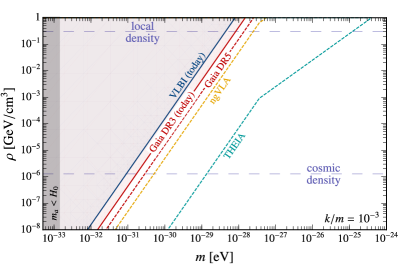
Figure 2: The sensitivity of astrometry to ultralight dark matter. Solid lines represent the potential of reanalyses of existing VLBI (solid blue) and Gaia DR3 (solid red) data to detect dark matter. Dashed lines project sensitivities for near-future data releases from Gaia DR5 (dashed red) and the next-generation Very Large Array (dashed yellow). The sensitivity of a search using THEIA, a proposed successor to Gaia, is shown in dashed teal. Details of the chosen parameters are discussed in the main text.

Detection Prospects and Discussion. To estimate the sensitivity of astrometric observations to dark matter, consider measurements of $N_{q}$ quasars, observed at regular time intervals $\Delta t$, for a total time $T$, with an instrumental uncertainty of $\sigma_{\theta}$. In the presence of dark matter, the apparent quasar locations exhibit correlated proper motions and modulations in their angular locations given by Eqs.(38) and (39). We estimate the sensitivity an optimal analysis for each search can have to dark matter using the log-likelihood ratio test in App. S-I. If no signal is present in the data, we find projected exclusion limits,

$$k\phi_{c}<\sigma_{\theta}\sqrt{\frac{6q_{\rm th}}{N_{q}}}\frac{1}{T}\sqrt{\frac{\Delta t}{T}}\,\,,\,\frac{v_{\rm o}k}{m}\phi_{c}<\sigma_{\theta}\sqrt{\frac{2q_{{\rm th}}}{N_{q}}}\sqrt{\frac{\Delta t}{T}}\,,$$ (40)

where $q_{\rm th}\simeq 2.7$ corresponds to a 95% upper limit. Our sensitivity expressions assume that only instrumental noise is present in the data and hence the signal can be completely distinguished from proper motion, secular aberration, and classical aberration. This could be done by exploiting the distance dependence of the dark matter-induced aberration; nearby sources could be used to “calibrate” the search, and quasars could be used to search for dark matter.

Measurements of 713 quasars were recently compiled with up to $1-10~{}\mu{\rm as}$-level precision per measurement from a combination of archival VLBI data and recent results from the Very Large Baseline Array (VLBA) Truebenbach and Darling (2017). The VLBA measurements represent a dramatic improvement in sensitivity, presenting a powerful opportunity to test for the existence of ultralight dark matter. To estimate the sensitivity achievable with current data, we assume $50$ well-measured quasars, each observed yearly with $5~{}\mu{\rm as}$ precision/measurement for ten years.

The sensitivity of VLBI will improve dramatically over time with an increasing number of measurements. Additionally, there will be a considerable gain in sensitivity if the next generation Very Large Array (ngVLA) project is constructed McKinnon and Selina (2018); Di Francesco et al. (2019); Kadler et al. (2023). Ref. Reid et al. (2018) suggested that ngVLA could measure $30$ times more sources while reaching $1~{}\mu{\rm as}$ sensitivity. To estimate the sensitivity of ngVLA, we assume $1000$ sources observed twice per year for a decade at this precision.

The Gaia space observatory measures a much larger set of extragalactic objects but with a precision of around 200 $\mu$as Gai . Gaia’s most recent DR3 data release amounts to 34 months of data with multiple measurements per extragalactic source, totaling approximately 1 million sources Gaia Collaboration et al. (2021). To estimate the sensitivity, we assume 10 measurements per source. For the full Gaia DR5 dataset, we assume a factor of two improvement in precision, $2\times 10^{6}$ sources, a 10-year dataset, and yearly measurements for each source. Looking further ahead, we also project the capabilities of a potential successor to Gaia, THEIA Malbet et al. (2022), assuming 100 measurements over 10 years with 1 $\mu$as for $10^{8}$ sources.

The projected sensitivities are shown in Fig. 2, fixing $k/m\sim 10^{-3}$ for concreteness. While this result is unlikely to hold for such light relics, our results can easily be rescaled to any velocity. A remarkable feature of astrometric dark matter searches is their sensitivity to ultralight relics. Indeed, at the lowest feasible dark matter mass, $m\simeq H_{0}$, we estimate that current Gaia DR3 data could discover dark matter with a density as low as $10^{-10}$ times the known local dark matter density.

Astrometry is complementary to cosmological probes of ultralight dark matter, which use a combination of cosmic microwave background and large-scale structure data to probe relics in a similar mass range Hlozek et al. (2015); Hložek et al. (2017); Hlozek et al. (2018); Laguë et al. (2022); Vogt et al. (2023); Rogers et al. (2023); Laguë et al. (2024). An astrometric search for dark matter would dramatically change the landscape of these efforts. Furthermore, astrometry could be used to probe Early Dark Energy Poulin et al. (2019, 2018); Smith et al. (2020); Hill et al. (2020), which typically also requires scalar fields in a similar mass range. Lastly, we note that by extending our analysis to the regime where $m\ll H_{0}$, we may be able to form a novel probe of quintessence Zlatev et al. (1999). We leave this for future work.

Acknowledgments. The authors would like to thank Lam Hui and Wei Xue for useful discussions on the density distribution of ultralight dark matter. We additionally thank Cristina Mondino for pointing out the importance of identifying a method of differentiating the signal from classical aberration.

Note Added. At the final stage of this work, we became aware of Ref. Kim (2024) which also considers astrometric deflection of light by dark matter.

S-I Sensitivity

In Eq. (40) we presented an expression for the sensitivity of a regular-cadence search to a secular proper motion and oscillations in the angular positions of quasars. In this section, we derive these expressions using the log-likelihood ratio test. Consider a single quasar whose position is measured with a Gaussian instrumental sensitivity $\sigma_{\theta}$, every $\Delta t$, for a total time span of $T$. We model the expected signal as a deterministic function, $\bar{\theta}(t)$, equal to $\omega_{\theta}t$ for a search for a secular proper motion and $\theta_{0}\cos(2\pi ft)$ for a search for an annual-modulation. The likelihood of $N_{t}$ measurements is,

$${\cal L}(\bar{\theta}|\left\{\theta_{j}\right\})=\frac{1}{(2\pi\sigma_{\theta}^{2})^{N_{t}/2}}\exp\left[-\frac{1}{2\sigma_{\theta}^{2}}\sum_{j=1}^{N_{t}}(\theta_{j}-\bar{\theta}(t_{j}))^{2}\right]\,.$$ (S-1)

The log-likelihood ratio between our signal model and background hypothesis ($\bar{\theta}=0$) is,

$$q\equiv\log\frac{{\cal L}(0|\left\{\theta_{j}\right\})}{{\cal L}(\bar{\theta}|\left\{\theta_{j}\right\})}=\frac{1}{2\sigma_{\theta}^{2}}\left[\sum_{j=1}^{N_{t}}(\theta_{j}-\bar{\theta}(t_{j}))^{2}-\theta_{j}^{2}\right]\,.$$ (S-2)

To determine the projected sensitivity, we employ the Asimov dataset Cowan et al. (2011), where the observed dataset is assumed to be given by the background-only hypothesis, $\theta_{j}=0$. In this case, the sums can be done analytically for both models. Assuming $T/\Delta t\gg 1$,

$$q\simeq\frac{1}{\sigma_{\theta}^{2}}\left\{\begin{array}[]{cc}\displaystyle\frac{\omega_{\theta}^{2}}{6}\frac{T^{3}}{\Delta t}\,,\\[10.0pt] \displaystyle\frac{\theta_{0}^{2}}{2}\frac{T}{\Delta t}\,.\end{array}\right.$$ (S-3)

We obtain our projected 95% confidence level limit by setting $q=q_{{\rm th}}\simeq 2.7$. For $N_{q}$ quasars, the experimental sensitivity grows as $1/\sqrt{N_{q}}$. This yields Eq. (40) in the main text.

References

- Khmelnitsky and Rubakov (2014) Andrei Khmelnitsky and Valery Rubakov, “Pulsar timing signal from ultralight scalar dark matter,” JCAP 02, 019 (2014), arXiv:1309.5888 [astro-ph.CO] .
- Porayko et al. (2018) Nataliya K. Porayko et al., “Parkes Pulsar Timing Array constraints on ultralight scalar-field dark matter,” Phys. Rev. D 98, 102002 (2018), arXiv:1810.03227 [astro-ph.CO] .
- Smarra et al. (2023) Clemente Smarra et al. (EPTA), “The second data release from the European Pulsar Timing Array: VI. Challenging the ultralight dark matter paradigm,” (2023), arXiv:2306.16228 [astro-ph.HE] .
- Afzal et al. (2023) Adeela Afzal et al. (NANOGrav), “The NANOGrav 15 yr Data Set: Search for Signals from New Physics,” Astrophys. J. Lett. 951, L11 (2023), arXiv:2306.16219 [astro-ph.HE] .
- Porayko and Postnov (2014) N. K. Porayko and K. A. Postnov, “Constraints on ultralight scalar dark matter from pulsar timing,” Phys. Rev. D 90, 062008 (2014), arXiv:1408.4670 [astro-ph.CO] .
- Graham et al. (2016) Peter W. Graham, David E. Kaplan, Jeremy Mardon, Surjeet Rajendran, and William A. Terrano, “Dark Matter Direct Detection with Accelerometers,” Phys. Rev. D 93, 075029 (2016), arXiv:1512.06165 [hep-ph] .
- Aoki and Soda (2016a) Arata Aoki and Jiro Soda, “Pulsar timing signal from ultralight axion in theory,” Phys. Rev. D 93, 083503 (2016a), arXiv:1601.03904 [hep-ph] .
- Aoki and Soda (2016b) Arata Aoki and Jiro Soda, “Detecting ultralight axion dark matter wind with laser interferometers,” Int. J. Mod. Phys. D 26, 1750063 (2016b), arXiv:1608.05933 [astro-ph.CO] .
- Blas et al. (2017) Diego Blas, Diana Lopez Nacir, and Sergey Sibiryakov, “Ultralight Dark Matter Resonates with Binary Pulsars,” Phys. Rev. Lett. 118, 261102 (2017), arXiv:1612.06789 [hep-ph] .
- De Martino et al. (2017) Ivan De Martino, Tom Broadhurst, S. H. Henry Tye, Tzihong Chiueh, Hsi-Yu Schive, and Ruth Lazkoz, “Recognizing Axionic Dark Matter by Compton and de Broglie Scale Modulation of Pulsar Timing,” Phys. Rev. Lett. 119, 221103 (2017), arXiv:1705.04367 [astro-ph.CO] .
- Kato and Soda (2020) Ryo Kato and Jiro Soda, “Search for ultralight scalar dark matter with NANOGrav pulsar timing arrays,” JCAP 09, 036 (2020), arXiv:1904.09143 [astro-ph.HE] .
- Nomura et al. (2020) Kimihiro Nomura, Asuka Ito, and Jiro Soda, “Pulsar timing residual induced by ultralight vector dark matter,” Eur. Phys. J. C 80, 419 (2020), arXiv:1912.10210 [gr-qc] .
- Kaplan et al. (2022) David E. Kaplan, Andrea Mitridate, and Tanner Trickle, “Constraining fundamental constant variations from ultralight dark matter with pulsar timing arrays,” Phys. Rev. D 106, 035032 (2022), arXiv:2205.06817 [hep-ph] .
- Xia et al. (2023) Zi-Qing Xia, Tian-Peng Tang, Xiaoyuan Huang, Qiang Yuan, and Yi-Zhong Fan, “Constraining ultralight dark matter using the Fermi-LAT pulsar timing array,” Phys. Rev. D 107, L121302 (2023), arXiv:2303.17545 [astro-ph.HE] .
- Luu et al. (2024) Hoang Nhan Luu, Tao Liu, Jing Ren, Tom Broadhurst, Ruizhi Yang, Jie-Shuang Wang, and Zhen Xie, “Stochastic Wave Dark Matter with Fermi-LAT -Ray Pulsar Timing Array,” Astrophys. J. Lett. 963, L46 (2024), arXiv:2304.04735 [astro-ph.HE] .
- Kim (2023) Hyungjin Kim, “Gravitational interaction of ultralight dark matter with interferometers,” JCAP 12, 018 (2023), arXiv:2306.13348 [hep-ph] .
- Hwang et al. (2024) Jai-chan Hwang, Donghui Jeong, Hyerim Noh, and Clemente Smarra, “Pulsar Timing Array signature from oscillating metric perturbations due to ultra-light axion,” JCAP 02, 014 (2024), arXiv:2311.00234 [astro-ph.CO] .
- Kim and Mitridate (2024) Hyungjin Kim and Andrea Mitridate, “Stochastic ultralight dark matter fluctuations in pulsar timing arrays,” Phys. Rev. D 109, 055017 (2024), arXiv:2312.12225 [hep-ph] .
- Brax et al. (2024) Philippe Brax, Clare Burrage, Jose A. R. Cembranos, and Patrick Valageas, “Detecting dark matter oscillations with gravitational waveforms,” (2024), arXiv:2402.04819 [astro-ph.CO] .
- Reid and Honma (2014) M. J. Reid and M. Honma, “Microarcsecond Radio Astrometry,” Ann. Rev. Astron. Astrophys. 52, 339–372 (2014), arXiv:1312.2871 [astro-ph.IM] .
- Thompson et al. (2017) A. Richard Thompson, James M. Moran, and Jr. Swenson, George W., Interferometry and Synthesis in Radio Astronomy, 3rd Edition (2017).
- Klioner (2003) Sergei A. Klioner, “A Practical Relativistic Model for Microarcsecond Astrometry in Space,” The Astronomical Journal 125, 1580–1597 (2003).
- Titov et al. (2011) O. Titov, S. B. Lambert, and A. M. Gontier, “VLBI measurement of the secular aberration drift,” Astron. Astrophys. 529, A91 (2011), arXiv:1009.3698 [astro-ph.CO] .
- Gaia Collaboration et al. (2021) Gaia Collaboration, S. A. Klioner, et al., “Gaia Early Data Release 3. Acceleration of the Solar System from Gaia astrometry,” Astronomy and Astrophysics 649, A9 (2021), arXiv:2012.02036 [astro-ph.GA] .
- Braginsky et al. (1990) V. B. Braginsky, N. S. Kardashev, I. D. Novikov, and A. G. Polnarev, “Propagation of electromagnetic radiation in a random field of gravitational waves and space radio interferometry,” Nuovo Cim. B 105, 1141–1158 (1990).
- Kaiser and Jaffe (1997) Nick Kaiser and Andrew H. Jaffe, “Bending of light by gravity waves,” Astrophys. J. 484, 545–554 (1997), arXiv:astro-ph/9609043 .
- Pyne et al. (1996) Ted Pyne, Carl R. Gwinn, Mark Birkinshaw, T. Marshall Eubanks, and Demetrios N. Matsakis, “Gravitational radiation and very long baseline interferometry,” Astrophys. J. 465, 566–577 (1996), arXiv:astro-ph/9507030 .
- Book and Flanagan (2011) Laura G. Book and Eanna E. Flanagan, “Astrometric Effects of a Stochastic Gravitational Wave Background,” Phys. Rev. D 83, 024024 (2011), arXiv:1009.4192 [astro-ph.CO] .
- Darling et al. (2018) Jeremy Darling, Alexandra E. Truebenbach, and Jennie Paine, “Astrometric Limits on the Stochastic Gravitational Wave Background,” Astrophys. J. 861, 113 (2018), arXiv:1804.06986 [astro-ph.IM] .
- Mihaylov et al. (2018) Deyan P. Mihaylov, Christopher J. Moore, Jonathan R. Gair, Anthony Lasenby, and Gerard Gilmore, “Astrometric Effects of Gravitational Wave Backgrounds with non-Einsteinian Polarizations,” Phys. Rev. D 97, 124058 (2018), arXiv:1804.00660 [gr-qc] .
- Garcia-Bellido et al. (2021) Juan Garcia-Bellido, Hitoshi Murayama, and Graham White, “Exploring the early Universe with Gaia and Theia,” JCAP 12, 023 (2021), arXiv:2104.04778 [hep-ph] .
- Fedderke et al. (2022) Michael A. Fedderke, Peter W. Graham, Bruce Macintosh, and Surjeet Rajendran, “Astrometric gravitational-wave detection via stellar interferometry,” Phys. Rev. D 106, 023002 (2022), arXiv:2204.07677 [astro-ph.IM] .
- Liang et al. (2023) Qiuyue Liang, Meng-Xiang Lin, Mark Trodden, and Sam S. C. Wong, “Probing Parity Violation in the Stochastic Gravitational Wave Background with Astrometry,” (2023), arXiv:2309.16666 [astro-ph.CO] .
- Kobayashi et al. (2017) Takeshi Kobayashi, Riccardo Murgia, Andrea De Simone, Vid Iršič, and Matteo Viel, “Lyman- constraints on ultralight scalar dark matter: Implications for the early and late universe,” Phys. Rev. D 96, 123514 (2017), arXiv:1708.00015 [astro-ph.CO] .
- Iršič et al. (2017) Vid Iršič, Matteo Viel, Martin G. Haehnelt, James S. Bolton, and George D. Becker, “First constraints on fuzzy dark matter from Lyman- forest data and hydrodynamical simulations,” Phys. Rev. Lett. 119, 031302 (2017), arXiv:1703.04683 [astro-ph.CO] .
- Nori et al. (2019) Matteo Nori, Riccardo Murgia, Vid Iršič, Marco Baldi, and Matteo Viel, “Lyman forest and non-linear structure characterization in Fuzzy Dark Matter cosmologies,” Mon. Not. Roy. Astron. Soc. 482, 3227–3243 (2019), arXiv:1809.09619 [astro-ph.CO] .
- Leong et al. (2019) Ka-Hou Leong, Hsi-Yu Schive, Ui-Han Zhang, and Tzihong Chiueh, “Testing extreme-axion wave-like dark matter using the BOSS Lyman-alpha forest data,” Mon. Not. Roy. Astron. Soc. 484, 4273–4286 (2019), arXiv:1810.05930 [astro-ph.CO] .
- Schutz (2020) Katelin Schutz, “Subhalo mass function and ultralight bosonic dark matter,” Phys. Rev. D 101, 123026 (2020), arXiv:2001.05503 [astro-ph.CO] .
- Nadler et al. (2021) E. O. Nadler et al. (DES), “Milky Way Satellite Census. III. Constraints on Dark Matter Properties from Observations of Milky Way Satellite Galaxies,” Phys. Rev. Lett. 126, 091101 (2021), arXiv:2008.00022 [astro-ph.CO] .
- Rogers and Peiris (2021) Keir K. Rogers and Hiranya V. Peiris, “Strong Bound on Canonical Ultralight Axion Dark Matter from the Lyman-Alpha Forest,” Phys. Rev. Lett. 126, 071302 (2021), arXiv:2007.12705 [astro-ph.CO] .
- Dalal and Kravtsov (2022) Neal Dalal and Andrey Kravtsov, “Excluding fuzzy dark matter with sizes and stellar kinematics of ultrafaint dwarf galaxies,” Phys. Rev. D 106, 063517 (2022), arXiv:2203.05750 [astro-ph.CO] .
- Foster et al. (2021) Joshua W. Foster, Yonatan Kahn, Rachel Nguyen, Nicholas L. Rodd, and Benjamin R. Safdi, “Dark Matter Interferometry,” Phys. Rev. D 103, 076018 (2021), arXiv:2009.14201 [hep-ph] .
- Dror et al. (2023) Jeff A. Dror, Stefania Gori, Jacob M. Leedom, and Nicholas L. Rodd, “Sensitivity of Spin-Precession Axion Experiments,” Phys. Rev. Lett. 130, 181801 (2023), arXiv:2210.06481 [hep-ph] .
- Maggiore (2018) Michele Maggiore, Gravitational Waves. Vol. 2: Astrophysics and Cosmology (Oxford University Press, 2018).
- Truebenbach and Darling (2017) Alexandra E. Truebenbach and Jeremy Darling, “The vlba extragalactic proper motion catalog and a measurement of the secular aberration drift,” The Astrophysical Journal Supplement Series 233, 3 (2017).
- McKinnon and Selina (2018) Mark McKinnon and Rob Selina, “The Next-Generation Very Large Array: Technical Overview,” in American Astronomical Society Meeting Abstracts #231, American Astronomical Society Meeting Abstracts, Vol. 231 (2018) p. 342.02.
- Di Francesco et al. (2019) James Di Francesco, Dean Chalmers, Nolan Denman, Laura Fissel, Rachel Friesen, Bryan Gaensler, Julie Hlavacek-Larrondo, Helen Kirk, Brenda Matthews, Christopher O’Dea, Tim Robishaw, Erik Rosolowsky, Michael Rupen, Sarah Sadavoy, Samar Sa-Harb, Greg Sivakoff, Mehrnoosh Tahani, Nienke van der Marel, Jacob White, and Christine Wilson, “The Next Generation Very Large Array,” in Canadian Long Range Plan for Astronomy and Astrophysics White Papers, Vol. 2020 (2019) p. 32, arXiv:1911.01517 [astro-ph.IM] .
- Kadler et al. (2023) M. Kadler et al., “A Collection of German Science Interests in the Next Generation Very Large Array,” (2023) arXiv:2311.10056 [astro-ph.IM] .
- Reid et al. (2018) M. Reid, L. Loinard, and T. Maccarone, “Astrometry and Long Baseline Science,” in Science with a Next Generation Very Large Array, Astronomical Society of the Pacific Conference Series, Vol. 517, edited by Eric Murphy (2018) p. 523, arXiv:1810.06577 [astro-ph.GA] .
- (50) “Cosmos esa,” https://www.cosmos.esa.int/web/gaia/science-performance, accessed: 04-15-2024.
- Malbet et al. (2022) Fabien Malbet et al., “Theia : science cases and mission profiles for high precision astrometry in the future,” in SPIE Astronomical Telescopes + Instrumentation 2022 (2022) arXiv:2207.12540 [astro-ph.IM] .
- Hlozek et al. (2015) Renée Hlozek, Daniel Grin, David J. E. Marsh, and Pedro G. Ferreira, “A search for ultralight axions using precision cosmological data,” Phys. Rev. D 91, 103512 (2015), arXiv:1410.2896 [astro-ph.CO] .
- Hložek et al. (2017) Renée Hložek, David J. E. Marsh, Daniel Grin, Rupert Allison, Jo Dunkley, and Erminia Calabrese, “Future CMB tests of dark matter: Ultralight axions and massive neutrinos,” Phys. Rev. D 95, 123511 (2017), arXiv:1607.08208 [astro-ph.CO] .
- Hlozek et al. (2018) Renée Hlozek, David J. E. Marsh, and Daniel Grin, “Using the Full Power of the Cosmic Microwave Background to Probe Axion Dark Matter,” Mon. Not. Roy. Astron. Soc. 476, 3063–3085 (2018), arXiv:1708.05681 [astro-ph.CO] .
- Laguë et al. (2022) Alex Laguë, J. Richard Bond, Renée Hložek, Keir K. Rogers, David J. E. Marsh, and Daniel Grin, “Constraining ultralight axions with galaxy surveys,” JCAP 01, 049 (2022), arXiv:2104.07802 [astro-ph.CO] .
- Vogt et al. (2023) Sophie M. L. Vogt, David J. E. Marsh, and Alex Laguë, “Improved mixed dark matter halo model for ultralight axions,” Phys. Rev. D 107, 063526 (2023), arXiv:2209.13445 [astro-ph.CO] .
- Rogers et al. (2023) Keir K. Rogers, Renée Hložek, Alex Laguë, Mikhail M. Ivanov, Oliver H. E. Philcox, Giovanni Cabass, Kazuyuki Akitsu, and David J. E. Marsh, “Ultra-light axions and the S 8 tension: joint constraints from the cosmic microwave background and galaxy clustering,” JCAP 06, 023 (2023), arXiv:2301.08361 [astro-ph.CO] .
- Laguë et al. (2024) Alex Laguë, Bodo Schwabe, Renée Hložek, David J. E. Marsh, and Keir K. Rogers, “Cosmological simulations of mixed ultralight dark matter,” Phys. Rev. D 109, 043507 (2024), arXiv:2310.20000 [astro-ph.CO] .
- Poulin et al. (2019) Vivian Poulin, Tristan L. Smith, Tanvi Karwal, and Marc Kamionkowski, “Early Dark Energy Can Resolve The Hubble Tension,” Phys. Rev. Lett. 122, 221301 (2019), arXiv:1811.04083 [astro-ph.CO] .
- Poulin et al. (2018) Vivian Poulin, Tristan L. Smith, Daniel Grin, Tanvi Karwal, and Marc Kamionkowski, “Cosmological implications of ultralight axionlike fields,” Phys. Rev. D 98, 083525 (2018), arXiv:1806.10608 [astro-ph.CO] .
- Smith et al. (2020) Tristan L. Smith, Vivian Poulin, and Mustafa A. Amin, “Oscillating scalar fields and the Hubble tension: a resolution with novel signatures,” Phys. Rev. D 101, 063523 (2020), arXiv:1908.06995 [astro-ph.CO] .
- Hill et al. (2020) J. Colin Hill, Evan McDonough, Michael W. Toomey, and Stephon Alexander, “Early dark energy does not restore cosmological concordance,” Phys. Rev. D 102, 043507 (2020), arXiv:2003.07355 [astro-ph.CO] .
- Zlatev et al. (1999) Ivaylo Zlatev, Li-Min Wang, and Paul J. Steinhardt, “Quintessence, cosmic coincidence, and the cosmological constant,” Phys. Rev. Lett. 82, 896–899 (1999), arXiv:astro-ph/9807002 .
- Kim (2024) Hyungjin Kim, “Astrometric Search for Ultralight Dark Matter,” (2024), to appear.
- Cowan et al. (2011) Glen Cowan, Kyle Cranmer, Eilam Gross, and Ofer Vitells, “Asymptotic formulae for likelihood-based tests of new physics,” Eur. Phys. J. C 71, 1554 (2011), [Erratum: Eur.Phys.J.C 73, 2501 (2013)], arXiv:1007.1727 [physics.data-an] .
SUPPLEMENTAL MATERIAL