Mpemba effects in open nonequilibrium quantum systems

Abstract

We generalize the classical thermal Mpemba effect (where an initially hot system relaxes faster to the final equilibrium state than a cold one) to open quantum systems coupled to several reservoirs. We show that, in general, two different types of quantum Mpemba effects are possible. They may be distinguished by quantum state tomography. However, the existence of a quantum Mpemba effect (without determining the type) can already be established by measuring simpler observables such as currents or energies. We illustrate our general results for the experimentally feasible case of an interacting two-site Kitaev model coupled to two metallic leads.

Introduction.—Quantum versions of the classical thermal Mpemba effect (ME) [1, 2] have attracted considerable recent attention, see, e.g., Refs. [3, 4, 5, 6, 7, 8, 9, 10, 11]. The classical ME arises when two copies of the same system are prepared in an equilibrium state at temperatures $T_{h}$ (“hot”) and $T_{c}$ (“cold”), respectively. For each copy, a sudden quench to the temperature $T_{\rm eq}<T_{c}<T_{h}$ is then performed. Measuring the relaxation times $\tau(T_{h/c})$ towards the final equilibrium configuration with temperature $T_{\rm eq}$, the ME takes place if the hot system relaxes faster than the cold one, i.e., for $\tau(T_{h})<\tau(T_{c})$. Similarly, the inverse ME is defined for $T_{c}<T_{h}<T_{\rm eq}$ by the condition $\tau(T_{c})<\tau(T_{h})$. Conventionally, the above relaxation times are determined by the respective times to undergo a phase transition, e.g., between water and ice [1], or between paramagnetic and ferromagnetic phases [12]. However, this definition does not apply to systems without phase transition. In general, the time needed to reach the final equilibrium state has to be extracted from a suitable “monitoring function” [2].

Different variants of quantum Mpemba effects (QMEs) have been proposed and studied during the past few years. The case of closed quantum systems has been addressed, e.g., in Refs. [3, 4, 11], where experimental observations are already available for trapped ions [5, 6]. We here instead investigate the QME for open nonequilibrium quantum systems coupled to (at least) two different reservoirs (“baths”), where the competition of stochastic relaxation processes and quantum effects drives the system towards a (nonequilibrium or equilibrium) stationary state, dubbed (N)ESS in what follows. In this Letter, we introduce a general protocol in order to unambiguously identify the QME in open nonequilibrium systems. Recent theoretical work in this context [7, 8, 9] proposed to search for (single or multiple) intersection points between time-dependent averages of some system observable computed at different temperatures. However, this definition is misleading and in conflict with previous work for the classical ME [13, 2]. In fact, for a poorly chosen monitoring function, it causes false QME identification and/or it misses cases where the QME actually occurs; for details, see the Supplementary Material (SM) [14]. Related work may violate the positivity of the density operator [10].

We here (i) formulate a general protocol for identifying and classifying the (direct or inverse) QME in open quantum systems connected to several baths (labeled by an index $\lambda$), and (ii) we illustrate this protocol for a relatively simple model which can be experimentally realized. In general, we consider a set of pre-quench bath parameters $\left\{p_{i}\right\}$. At time, say, $t=0$, one performs a quench to the after-quench parameters $\{p_{i,{\rm(N)ESS}}\}$ describing the final (N)ESS configuration. The above parameter sets may include, e.g., the chemical potentials $\mu_{\lambda}$ and thermal energies $k_{B}T_{\lambda}$ of the different baths. We next extend the notion of hot vs cold initial configurations [1] to “far” vs “close” initial conditions ($\{p_{i,f}\}$ vs $\{p_{i,c}\}$). This allows one to describe more general cases where several control parameters are changed. For fixed after-quench parameters, we use a Euclidean distance in this parameter space,

$$\mathcal{D}_{E}\left(\left\{p_{i}\right\}\right)=\sqrt{\sum_{i}\left(p_{i}-p_{i,{\rm(N)ESS}}\right)^{2}}.$$ (1)

For $\mathcal{D}_{E}(\left\{p_{i,c}\right\})<\mathcal{D}_{E}(\left\{p_{i,f}\right\})$, the set $\{p_{i,c}\}$ is considered to be closer to $\{p_{i,{\rm(N)ESS}}\}$ than the set $\{p_{i,f}\}$. Below we also employ the trace distance [15],

$$\mathcal{D}_{T}\left(\rho(t)\right)=\frac{1}{2}\mathrm{Tr}\left|\rho(t)-\rho_{\rm(N)ESS}\right|,$$ (2)

which is a measure of the distance between the system density matrix $\rho(t)$ and the final (N)ESS state $\rho_{\rm(N)ESS}$.

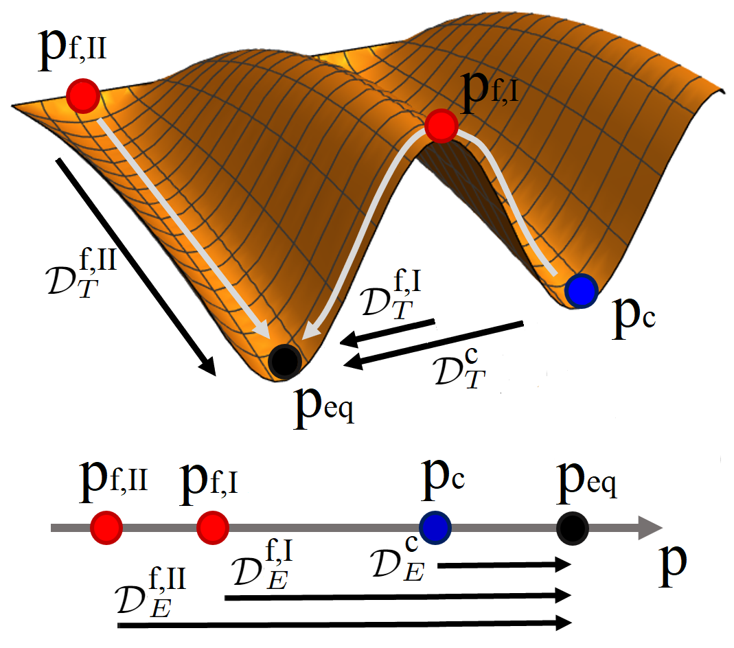
Figure 1: Upper panel: Schematic sketch of the energy landscape in state space and the corresponding time-evolution trajectories for type-I and type-II QMEs, respectively. The trace distance (2) between different initial states and the final (N)ESS density matrix (corresponding to $\{p_{\rm eq}\}$) is indicated. We consider “far” ($\{p_{i,f}\}$) and “close” ($\{p_{i,c}\})$ initial configurations, cf. the lower panel. For a type-I QME, the trace distance (2) satisfies $\mathcal{D}_{T}(\rho_{f}(t))<\mathcal{D}_{T}(\rho_{c}(t))$ at all times. For the more elusive type-II QME, we instead have $\mathcal{D}_{T}(\rho_{f}(t))>\mathcal{D}_{T}(\rho_{c}(t))$ at short times $t<t^{*}$, but the inequality is reversed at longer times. Lower panel: In both type-I and type-II cases, $\mathcal{D}_{E}(\left\{p_{i,f}\right\})>\mathcal{D}_{E}(\left\{p_{i,c}\right\})$, see Eq. (1), which defines far vs close initial configurations.

Two definitions for the classical ME have been introduced in Refs. [2, 13], which we here unify and extend to the quantum case, see Fig. 1. We label them as type-I and type-II QME. In both cases, the two initial configurations (far vs close) satisfy $\mathcal{D}_{E}(\left\{p_{i,f}\right\})>\mathcal{D}_{E}(\left\{p_{i,c}\right\})$, see Eq. (1). For the type-I QME, the initially far system $\{p_{i,f}\}$ reaches the final (N)ESS faster because the corresponding state $\rho_{f}(0)$ is actually closer to $\rho_{\rm(N)ESS}$, i.e., $\mathcal{D}_{T}(\rho_{f}(0))<\mathcal{D}_{T}(\rho_{c}(0))$, see Eq. (2). It thus enjoys a natural advantage over the nominally closer system during the ensuing time evolution [13]. For the more elusive type-II QME, the far vs close systems evolve through different paths but even though $\rho_{c}(0)$ is nearer to the (N)ESS state, i.e., $\mathcal{D}_{T}(\rho_{f}(0))>\mathcal{D}_{T}(\rho_{c}(0))$, the path that connects the far system to the (N)ESS is eventually shorter [2]. By analyzing both $\mathcal{D}_{T}(\rho(t))$ as a function of time as well as $\mathcal{D}_{E}(\left\{p_{i}\right\})$, both types of QME can be unambiguously identified.

Our protocol avoids any false QME detection or mislead since the trace distance (2), which is in the range $\left[0,1\right]$, is a monotonically decreasing function of time under Lindblad dynamics [16]. In particular, (a) if $\mathcal{D}_{T}(\rho_{f}(t))>\mathcal{D}_{T}(\rho_{c}(t))$ for all times, no QME takes place; (b) if $\mathcal{D}_{T}(\rho_{f}(t))<\mathcal{D}_{T}(\rho_{c}(t))$ for all times, we have a type-I QME; and (c) if $\mathcal{D}_{T}(\rho_{f}(0))>\mathcal{D}_{T}(\rho_{c}(0))$ but a finite time $t^{*}$ exists such that $\mathcal{D}_{T}(\rho_{f}(t))<\mathcal{D}_{T}(\rho_{c}(t))$ for $t>t^{*}$, a type-II QME takes place. Below we illustrate both types of QME for a simple and experimentally accessible model, where we outline concrete experimental protocols. By measuring time-dependent currents, one can unambiguously establish the existence or absence of the QME. In order to distinguish both types of QME, however, quantum state tomography becomes necessary.

Model.—We consider the minimal interacting two-site Kitaev model (I2KM) [17, 18] with a non-local Coulomb interaction strength $U$ [19] (we put $\hbar=k_{B}=1$ below),

$$H_{\rm{I2KM}} = \epsilon_{1}n_{1}+\epsilon_{2}n_{2}+Un_{1}n_{2}$$

$$+ t_{h}(c_{1}^{\dagger}c_{2}+c^{\dagger}_{2}c_{1})+\Delta c_{1}^{\dagger}c_{2}^{\dagger}+\Delta^{*}c_{2}c_{1},$$

where $c_{i}$ and $n_{i}=c_{i}^{\dagger}c_{i}$ are spinless electron annihilation and occupation number operators for site (quantum dot) $i\in\{1,2\}$, respectively. The $\epsilon_{i}$ are on-site energies, $t_{h}$ is the tunneling amplitude connecting the two dots, and $\Delta$ is a superconducting pairing amplitude due to crossed Andreev reflection processes. Without loss of generality, we assume $t_{h}$ real-valued. Both $t_{h}$ and $\Delta$ can be mediated by a short superconductor, while the on-site energies may be controlled by voltages applied to finger gates. The I2KM has recently been studied experimentally in the context of realizing “poor man’s” Majorana bound states [20, 21]. We therefore expect that our predictions on the QME can be readily put to a test. Using the many-body state basis

$$\{\lvert 0\rangle,\,\lvert 1\rangle=c_{1}^{\dagger}\lvert 0\rangle,\,\lvert 2\rangle=c_{2}^{\dagger}\lvert 0\rangle,\,\lvert d\rangle=c_{1}^{\dagger}c_{2}^{\dagger}\lvert 0\rangle\},$$ (4)

Eq. (Mpemba effects in open nonequilibrium quantum systems) is equivalently expressed as $4\times 4$ matrix,

$$H_{\rm I2KM}=\left(\begin{array}[]{cccc}0&0&0&\Delta^{*}\\ 0&\epsilon_{1}&t_{h}&0\\ 0&t_{h}&\epsilon_{2}&0\\ \Delta&0&0&\epsilon_{d}\end{array}\right),$$ (5)

with $\epsilon_{d}=\epsilon_{1}+\epsilon_{2}+U$. The states $|0\rangle$ and $|d\rangle$ have even fermion parity, while $|1\rangle$ and $|2\rangle$ have odd parity.

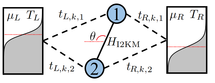
Figure 2: Sketch of the studied setup. Two quantum dots (blue circles) described by $H_{\rm I2KM}$, see Eqs. (Mpemba effects in open nonequilibrium quantum systems) and (5), are coupled to left and right ($\lambda=L,R$) metallic leads (Fermi gases) with the respective temperature $T_{\lambda}$ and chemical potential $\mu_{\lambda}$. Fermi distributions in both leads are schematically indicated, with $\mu_{\lambda}$ shown as red dotted lines. Electrons with momentum $k$ in lead $\lambda$ are tunnel-coupled to dot $i\in\{1,2\}$ with amplitude $t_{\lambda,k,i}$. The angle $\theta$ defines the relative position between the two dots compared to the leads.

Next, as illustrated in Fig. 2, the I2KM is coupled to left and right $(\lambda=L,R)$ metallic leads by tunnel contacts ($H_{c})$. Describing the leads by noninteracting fermions ($H_{l}$) with chemical potential $\mu_{\lambda}$ and temperature $T_{\lambda}$, the total Hamiltonian is $H=H_{\rm{I2KM}}+H_{l}+H_{c}$ with $H_{l}=\sum_{\lambda,k}\epsilon_{k}c_{\lambda,k}^{\dagger}c_{\lambda,k}$ and $H_{c}=\sum_{\lambda,k,i}(t_{\lambda,k,i}c_{\lambda,k}^{\dagger}c_{i}+\text{h.c.})$. Here $c_{\lambda,k}$ are electron annihilation operators for lead $\lambda$ and momentum $k$ (with dispersion $\epsilon_{k})$, and $t_{\lambda,k,i}$ is a tunneling amplitude connecting the respective lead electron to dot $i$. The relative orientation of the two dots with respect to the leads is encoded by an angle $\theta$ as illustrated in Fig. 2. For instance, for $\theta=0$, the two dots are aligned “in series” with the leads.

Lindblad equation.—For weak tunnel couplings $t_{\lambda,k,i}$, a Lindblad master equation is expected to describe the time evolution of the I2KM density matrix $\rho(t)$ [22, 23, 24, 25]. Integrating out the leads in the wide-band approximation where the bandwidth of the leads exceeds all system energy scales [26, 27, 28], and applying the standard Born-Markov and rotating wave approximations [29], we indeed obtain a Lindblad equation,

$$\partial_{t}\rho=-i\left[H_{\mathrm{I2KM}},\rho\right]+\sum_{m\neq n}\Gamma_{m,n}\,{\cal L}\left[L_{m,n}\right]\rho,$$ (6)

with the dissipator ${\cal L}[L]\rho=L\rho L^{\dagger}-\frac{1}{2}\{L^{\dagger}L,\rho\}$ and the anticommutator $\{\cdot,\cdot\}$. For a given jump operator $L_{m,n}=\lvert m\rangle\langle n\rvert$, with $m$ and $n$ running over the I2KM many-body states in Eq. (4), $\Gamma_{m,n}=\sum_{\lambda=L,R}\Gamma_{m,n}^{\lambda}$ denotes the corresponding transition rate. Within the Lindblad approach, the leads only inject (or remove) a single electron into (from) the I2KM at a given time. Hence the non-vanishing transition rates in Eq. (6) only connect states in different parity sectors, $\{\lvert 0\rangle,\lvert d\rangle\}\leftrightarrow\{\lvert 1\rangle,\lvert 2\rangle\}$. On the other hand, the Hamiltonian contribution in Eq. (6) due to $H_{\mathrm{I2KM}}$ only connects states within the same parity sector, $\lvert 1\rangle\leftrightarrow\lvert 2\rangle$ or $\lvert 0\rangle\leftrightarrow\lvert d\rangle$, see Eq. (5). We find the non-vanishing rate contributions ($i=1,2$)

$$\Gamma^{\lambda}_{i,0}=\gamma_{\lambda,i}(\epsilon_{i})f_{\lambda}(\epsilon_{i}),\quad\Gamma_{d,i}^{\lambda}=\gamma_{\lambda,3-i}(\epsilon_{d}-\epsilon_{i})f_{\lambda}(\epsilon_{d}-\epsilon_{i}),$$ (7)

together with the detailed balance relations

$$\Gamma^{\lambda}_{i,0}/\Gamma^{\lambda}_{0,i}=e^{-(\epsilon_{i}-\mu_{\lambda})/T_{\lambda}},\quad\Gamma^{\lambda}_{d,i}/\Gamma^{\lambda}_{i,d}=e^{-(\epsilon_{d}-\epsilon_{i}-\mu_{\lambda})/T_{\lambda}},$$ (8)

with $f_{\lambda}(\epsilon)=[e^{(\epsilon-\mu_{\lambda})/T_{\lambda}}+1]^{-1}$ and $\gamma_{\lambda,i}(\epsilon)=2\pi\nu_{\lambda}(\epsilon)\,|t_{\lambda,i}(\epsilon)|^{2}$, where $t_{\lambda,i}(\epsilon_{k})=t_{\lambda,k,i}$ and the lead density of states is $\nu_{\lambda}(\epsilon)$. Below, following standard arguments [26], the rates $\gamma_{\lambda,i}(\epsilon)=\gamma_{\lambda,i}$ in Eq. (7) are assumed energy-independent. For simplicity, we parameterize them as

$$\gamma_{L,1}=\gamma_{R,2}=\frac{\Gamma}{2}(1+\cos\theta),\quad\gamma_{L,2}=\gamma_{R,1}=\frac{\Gamma}{2}(1-\cos\theta),$$ (9)

with the angle $\theta$ in Fig. 2. For each lead $\lambda$, the total hybridization strength is thus assumed independent of $\theta$ and $\lambda$, i.e., $\gamma_{\lambda,1}+\gamma_{\lambda,2}=\Gamma$.

Dynamics.—The presence of two independent electron reservoirs renders the system evolution richer than in the standard single-bath case. If the two baths have the same chemical potential and the same temperature, the I2KM is driven towards a thermal ESS for $t\to\infty$, with zero net current flowing between the leads. On the contrary, for $\left\{\mu_{L},T_{L}\right\}\neq\left\{\mu_{R},T_{R}\right\}$, the system evolves towards a current-carrying NESS with a time-independent steady-state density matrix. For the time-dependent I2KM state $\rho(t)$, the net current from lead $\lambda$ to the I2KM is given by $I^{\rm tot}_{\lambda}=I^{\rm in}_{\lambda}-I^{\rm out}_{\lambda}$, where

$$I^{\rm in}_{\lambda} = \sum_{i=1,2}\left[\gamma_{\lambda,i}f_{\lambda}(\epsilon_{i})\rho_{0,0}+\gamma_{\lambda,3-i}f_{\lambda}(\epsilon_{d}-\epsilon_{i})\rho_{i,i}\right],$$

$$I^{\rm out}_{\lambda} = \sum_{i}\left[\gamma_{\lambda,i}\bar{f}_{\lambda}(\epsilon_{i})\rho_{i,i}+\gamma_{\lambda,3-i}\bar{f}_{\lambda}(\epsilon_{d}-\epsilon_{i})\rho_{d,d}\right]$$ (10)

with $\bar{f}_{\lambda}(\epsilon)=1-f_{\lambda}(\epsilon)$ and $\rho_{m,n}$ the density matrix elements in the many-body state basis in Eq. (4). Similarly, the current $I_{1,2}$ between the two dots and the I2KM energy $E$ are defined as

$$I_{1,2}=-it_{h}\left(\rho_{2,1}-\rho_{1,2}\right),\quad E=\mathrm{Tr}\left(\rho H_{\rm I2KM}\right).$$ (11)

All the above quantities can be used to monitor the time evolution of the I2KM.

For a numerical solution, Eq. (6) is expressed in the equivalent superoperator representation, $\partial_{t}\hat{\rho}={\bf M}\hat{\rho}$, where $\hat{\rho}$ is a $16$-component vector, i.e. the vectorized form of the $4\times 4$ density matrix and ${\bf M}$ a $16\times 16$ matrix [29]. For given initial state ${\hat{\rho}}(t=0)$, this differential equation system is solved by ($\alpha=1,\ldots,16$)

$${\hat{\rho}}_{\alpha}(t)=\sum_{\beta,\eta=1}^{16}e^{\lambda_{\beta}t}R_{\alpha,\beta}L_{\beta,\eta}\,\hat{\rho}_{\eta}(0),$$ (12)

with the eigenvalues $\lambda_{\beta}$ and the corresponding right and left eigenvectors $\mathbf{R}_{\beta}$ and $\mathbf{L}_{\beta}$ of ${\bf M}$. The time evolution of the system now sensitively depends on the eigenvalues $\lambda_{\beta}$. On general grounds, the real parts of all $\lambda_{\beta}$ are non-positive (the Lindblad equation describes a relaxation dynamics), and complex eigenvalues form complex conjugate pairs (arising from the system Hamiltonian). Eigenvalues with ${\rm Re}(\lambda_{\beta})<0$ describe exponential decay, while ${\rm Im}(\lambda_{\beta})\neq 0$ results in damped (spiral path) or undamped (elliptic path) oscillations [30, 31]. If all states are accessible to the Lindblad dynamics in Eq. (6), either because of the dissipative transition rates $\Gamma_{m,n}$ or because of the unitary dynamics due to $H_{\rm I2KM}$, at least one eigenvalue $\lambda=0$ exists. This eigenvalue corresponds to the (N)ESS, $\hat{\rho}_{\rm(N)ESS}=\hat{\rho}(t\to\infty)$ with $\partial_{t}{\hat{\rho}}_{\rm(N)ESS}=0$. In principle, several eigenvalues may vanish, causing a (N)ESS manifold, where the final state depends on the initial condition [32, 33]. If the dissipative rates $\Gamma_{m,n}$ can already mix all system states by themselves, a closed set of equations holds for the populations only, i.e., for the diagonal elements of the density matrix [14]. These equations only depend on the jump operators and not on the Hamiltonian, giving rise to a purely exponential decay. However, if the dissipative rates cannot trigger all possible system transitions, as is the case in our system, a competition between coherent Hamiltonian evolution and incoherent dissipative evolution takes place. Then the coupled equations for the full density matrix must be solved.

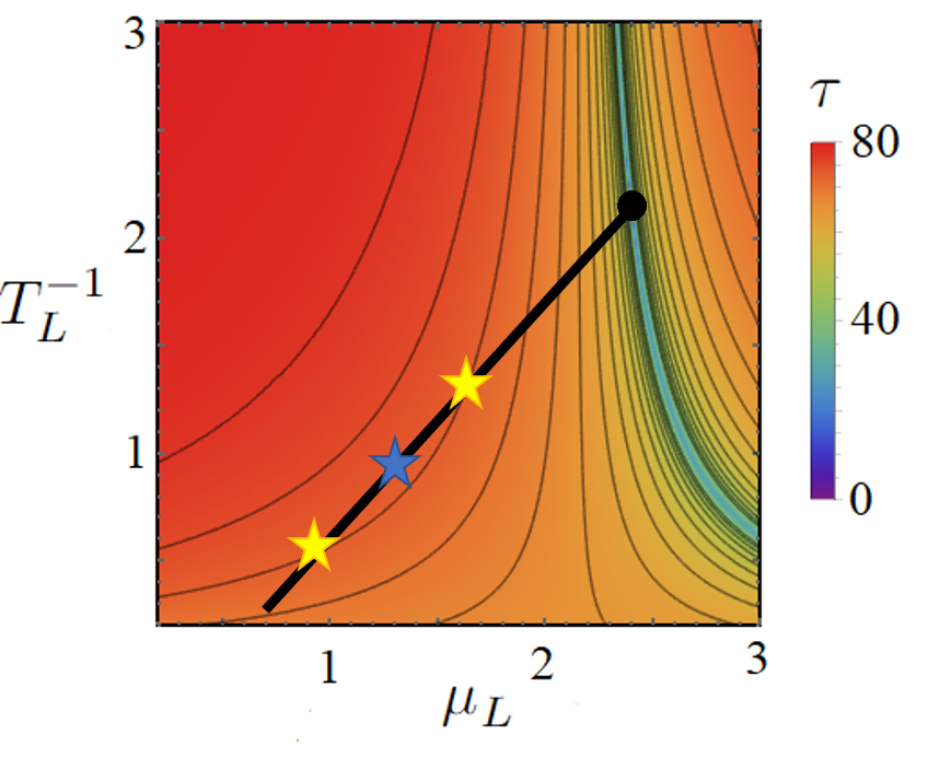
Figure 3: Color-scale plot of the I2KM relaxation time $\tau$ towards the ESS (indicated by a black circle) in the $T_{L}^{-1}$-$\mu_{L}$ plane for different initial NESS configurations $(T^{-1}_{L},\mu_{L})$, where $(T^{-1}_{R},\mu_{R})$ is identical to the final ESS parameters, $T^{-1}_{\lambda,{\rm ESS}}=2.15$ and $\mu_{\lambda,{\rm ESS}}=2.4$ for $\lambda=L,R$. Other parameters are $t_{h}=1$, $\epsilon_{1}=\epsilon_{2}=2$, $\Delta=0.1$, $U=0.25$, $\Gamma=0.1$, and $\theta=0$. (A non-zero phase for $\Delta$ has no significant effect on the QME.) Thin black curves indicate $\tau$-isolines. Yellow and blue stars (located on a thick black line connected with the ESS) denote initial states discussed in the main text.

Observing the QME.—We now discuss typical results for the above model, which were obtained by numerically solving Eq. (6). Additional results can be found in the SM [14]. We here focus on a specific I2KM parameter set and show the relaxation time $\tau$ from different initial states towards a fixed final ESS configuration in Fig. 3. Here $\tau$ was obtained from the time dependence of the trace distance (2). Figure 3 shows a color-scale plot of $\tau$ in the $T_{L}^{-1}$-$\mu_{L}$ plane, where initial NESS configurations are defined by $(T^{-1}_{L},\mu_{L})$, with $(T^{-1}_{R},\mu_{R})$ identical as for the ESS. Let us first focus on the two initial states marked by yellow stars in Fig. 3. Both states are located on a $\tau$-isoline and thus have the same relaxation time even though the state at $(T_{L,f}^{-1},\mu_{L,f})=(0.5,0.9)$ on the lower left side is further away from the ESS, as measured by ${\cal D}_{E}$ in Eq. (1). We compare this state to the initial state $(T_{L,c}^{-1},\mu_{L,c})$ marked by a blue star in Fig. 3 which has a longer relaxation time $\tau$ even though it clearly is closer to the ESS. We thus conclude that the QME takes place. Comparing instead the other initial state marked by a yellow star to the one marked by the blue star, no QME occurs.

In order to decide which type of QME occurs, one needs to analyze the time dependence of the trace distance ${\cal D}_{T}$ in Eq. (2). As shown in Fig. 4(a), depending on the parameter regime, one can either realize a type-I QME or the more elusive type-II QME. The latter is characterized by an intersection point at a finite time $t^{*}$. We further discuss this point in the SM [14], where we compare the isolines of the trace distance (2) at $t=0$ to those of the Euclidean distance (1). However, in order to obtain curves such as those in Fig. 4(a) in experiments, one has to perform quantum state tomography. A much less costly way to identify the QME is to measure the time-dependent currents (10), as we illustrate in Fig. 4(b). Alternatively, one can also the quantities in Eq. (11) [14]. However, a measurement of the current (10) or of the observables in Eq. (11) is not sufficient to differentiate between type-I and type-II QMEs. The latter distinction appears to require state tomography.

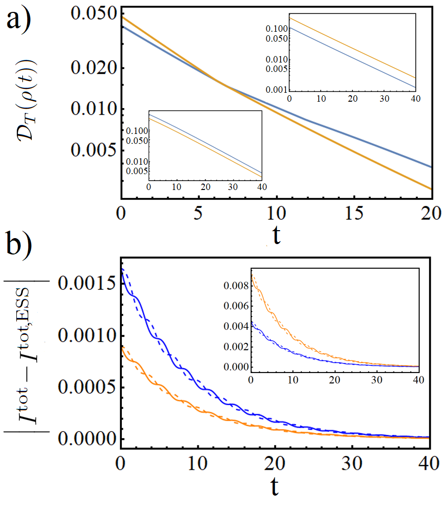
Figure 4: Examples for QMEs for the I2KM with parameters as specified in Fig. 3. Yellow [blue] curves refer to the “far” [“close”] initial state $\rho_{f}(0)$ [$\rho_{c}(0)$] as defined by ${\cal D}_{E}$ in Eq. (1). Panel (a): Trace distance ${\cal D}_{T}$ vs time $t$, for three different cases as discussed in the Introduction. Note the logarithmic scales for ${\cal D}_{T}$. The main panel shows a type-II QME, where $(T_{L,c}^{-1},\mu_{L,c})=(0.7,2.7)$ and $(T_{L,f}^{-1},\mu_{L,f})=(0.7,3)$. The lower left inset shows a type-I QME, with $(T_{L,c}^{-1},\mu_{L,c})=(1.3,1.5)$ and $(T_{L,f}^{-1},\mu_{L,f})=(0.7,1.5)$. The upper right inset shows a case without QME, where $(T_{L,c}^{-1},\mu_{L,c})=(1.7,2.7)$ and $(T_{L,f}^{-1},\mu_{L,f})=(1.7,3)$. Panel (b): Current differences $\left|I_{\lambda}^{\rm tot}(t)-I^{\rm tot,ESS}\right|$ vs time $t$, see Eq. (10). Solid (dashed) curves correspond to currents from lead $\lambda=L$ ($\lambda=R$), where the final ESS value does not depend on $\lambda$. The states $\rho_{f,c}(t)$ shown in the main panel describe a type-I QME, with the same parameters as in the lower left inset of panel (a). The inset shows results in the absence of a QME, cf. the upper right inset of panel (a).

Conclusions.—We have formulated a general protocol which allows one to unambiguously identify and classify the QME in open nonequilibrium quantum systems. Our approach shows that quantum correlations are of fundamental importance for the predicted phenomena. As practical example, we have applied our ideas to a minimal interacting two-site Kitaev model, which has recently been studied experimentally. In principle, our approach can be readily generalized to more complicated open topological systems in one and two dimensions [34, 35, 36, 37]. While the distinction of type-I and type-II QMEs in general requires quantum state tomography, one can infer the existence of a QME already by monitoring the time dependence of simpler observables such as the electrical current.

I Supplemental Material

We here provide further details on our work. In Sec. I, we comment on previous theories for the quantum Mpemba effect (QME) in open nonequilibrium systems which suggest to employ finite-time crossing points of certain observables for identifying the QME. We also compare their predictions to those made by our protocol. In Sec. II, we provide further details on experimentally accessible quantities for the interacting two-site Kitaev model (I2KM) discussed in the main text. In Sec. III, we comment on the optimal working conditions and on the role of the geometric angle $\theta$ of the I2KM. Finally, in Sec. IV, we discuss the sweet parameter spot of the I2KM, where one has fine-tuned Majorana bound states. For brevity, Eq. (X) in the main text is referred to as Eq. (MX) below.

II I. Crossing points

In recent theoretical work [7, 8, 9], the QME has been linked to finite-time crossings of temporal trajectories of certain observables. Such finite-time crossings are searched for in various physical quantities, using two system copies with different initial (hot vs cold) parameters but the same after-quench (N)ESS parameters. Typical observables include the diagonal elements of the system density matrix (“populations”), an effective temperature, the von Neumann entropy, and the average system energy. However, all those quantities are neither bounded from above or below, and they are generally not monotonically decreasing (or increasing) functions of time. For this reason, they can cause false detection of the QME or overlook the QME when it is actually present. We note that related arguments have already been given in Ref. [2] for the classical (thermal) equilibrium ME. In the following, we argue that the existence of one or multiple crossing points is neither a necessary nor a sufficient condition for the onset of the QME.

In Ref. [7], a spinful interacting quantum dot (ISD) coupled to two leads has been considered. The total Hamiltonian, $H=H_{\rm{ISD}}+H_{l}+H_{c}$, contains the ISD Hamiltonian,

$$H_{\rm{ISD}}=\sum_{\sigma}\epsilon\,n_{\sigma}+Un_{\uparrow}n_{\downarrow},$$ (13)

where $c_{\sigma}$ and $n_{\sigma}=c_{\sigma}^{\dagger}c_{\sigma}$ are electron annihilation and occupation operators for spin $\sigma\in\{\uparrow,\downarrow\}$, respectively. Here $\epsilon$ is a single-particle energy and $U$ the Coulomb charging energy. Below, we use the many-body basis

$$\{\lvert 0\rangle,\,\lvert\uparrow\rangle=c_{\uparrow}^{\dagger}|0\rangle,\,\lvert\downarrow\rangle=c_{\downarrow}^{\dagger}|0\rangle,\,\lvert d\rangle=c_{\uparrow}^{\dagger}c_{\downarrow}^{\dagger}\lvert 0\rangle\},$$ (14)

which diagonalizes the Hamiltonian (13). The Hamiltonian $H_{l}$ describes the left and right ($\lambda=L,R$) leads as spin-degenerate ideal Fermi gases, similar to the main text. The tunneling Hamiltonian $H_{c}$ connecting the leads and the ISD is given by

$$H_{c}=\sum_{\lambda,k,\sigma}t_{\lambda}c_{\lambda,k,\sigma}^{\dagger}c_{\sigma}+\textrm{h.c.},$$ (15)

where $c_{\lambda,k,\sigma}$ is the electron annihilation operator for lead $\lambda$, momentum $k$, and spin $\sigma$. Following Ref. [7], the tunneling amplitude $t_{\lambda}$ between lead $\lambda$ and the ISD is assumed spin- and energy-independent.

In the wide-band approximation, and using the Born-Markov and rotating wave approximations, one can integrate out the leads and derive a Lindblad master equation for the density matrix $\rho(t)$ of the ISD model. We express $\rho$ as $4\times 4$ matrix in the basis (14). In contrast to the I2KM, the dissipative jump operators mix all system states for the ISD model. As a consequence, the dynamical equations for the diagonal elements of the density matrix (i.e., the populations),

$${\bf P}(t)\equiv\left(\begin{array}[]{c}\rho_{0,0}(t)\\ \rho_{\uparrow,\uparrow}(t)\\ \rho_{\downarrow,\downarrow}(t)\\ \rho_{d,d}(t)\end{array}\right),$$ (16)

decouple from the off-diagonal entries of $\rho(t)$. (For simplicity, we assume that one starts initially with a diagonal state $\rho(0)$.) One then arrives at a Pauli master equation for the populations [29],

$$\partial_{t}{\bf P}(t)={\bf M}\,{\bf P}(t),$$ (17)

where ${\bf M}$ is given by the $4\times 4$ matrix

$$\left(\begin{array}[]{cccc}-\sum_{\sigma}\Gamma_{\sigma,0}&\Gamma_{0,\uparrow}&\Gamma_{0,\downarrow}&0\\ \Gamma_{\uparrow,0}&-\Gamma_{d,\uparrow}-\Gamma_{0,\uparrow}&0&\Gamma_{\uparrow,d}\\ \Gamma_{\downarrow,0}&0&-\Gamma_{d,\downarrow}-\Gamma_{0,\downarrow}&\Gamma_{\downarrow,d}\\ 0&\Gamma_{d,\uparrow}&\Gamma_{d,\downarrow}&-\sum_{\sigma}\Gamma_{\sigma,d}\end{array}\right).$$ (18)

We use the rates

$$\Gamma_{\sigma,0} = \gamma\sum_{\lambda=L,R}f_{\lambda}(\epsilon)=2\gamma-\Gamma_{0,\sigma},$$

$$\Gamma_{d,\sigma} = \gamma\sum_{\lambda}f_{\lambda}(\epsilon+U)=2\gamma-\Gamma_{\sigma,d},$$ (19)

where $f_{\lambda}(\epsilon)$ is the Fermi function and $\gamma=2\pi\nu_{\lambda}(\epsilon)|t_{\lambda}|^{2}$ as in the main text. The microscopic transition rate $\gamma$ is assumed to be independent of energy, spin, and the lead index [7].

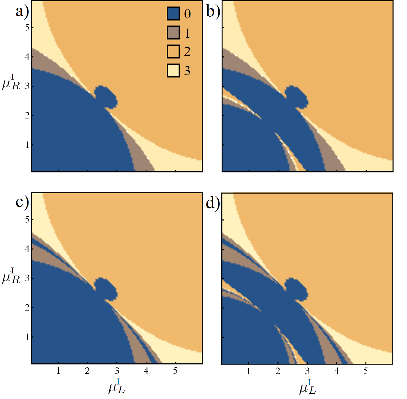
Figure 5: Phase diagram for the ISD model in the $\mu_{R}^{I}$-$\mu_{L}^{I}$ plane for otherwise fixed parameters, cf. Ref. [7]. Two copies of the system are initially (at time $t=0$) prepared in the equilibrium density matrix corresponding to $(\mu_{L}^{I},\mu_{R}^{I}$) with $\beta_{L}^{I}=\beta_{R}^{I}=1.15$, and $\mu_{L}^{II}=\mu_{R}^{II}=2.43$ with $\beta_{L}^{II}=\beta_{R}^{II}=1.15$, respectively. After the quench, the left and right leads have chemical potentials $\mu_{L}^{\rm ESS}=\mu_{R}^{\rm ESS}=2$ and inverse temperatures $\beta_{L}^{\rm ESS}=\beta_{R}^{\rm ESS}=1$. The other parameters are set to $U=1.25$, $\epsilon=2$, and $\gamma=1$. (a): Number of populations $P_{\eta}$, see Eq. (16), exhibiting a crossing point for a finite time $t^{*}$ as a function of $\mu_{L}^{I}$ and $\mu_{R}^{I}$. (b): Same as panel (a) but applying a cut-off scheme to account for a finite measurement resolution. Here, crossing points are discarded if $\left|P_{\eta}^{I/II}(t^{*})-P_{\eta}^{\rm ESS}\right|<10^{-5}$. (c): Crossing points are now instead searched for by analyzing $\left|P_{\eta}(t)-P_{\eta}^{\rm ESS}\right|$, see Ref. [7]. (d): Same as in panel (c) but with the analogous cut-off procedure as applied in panel (b).

In Ref. [7], the following protocol to search for the QME has been introduced. Two copies of the system (labeled by $I$ and $II$, respectively) are prepared in the equilibrium configuration ${\bf P}^{I(II)}(0)$, defined by the chemical potentials and inverse temperatures of both leads, $\left\{\mu_{L}^{I(II)},\mu_{R}^{I(II)},\beta_{L}^{I(II)},\beta_{R}^{I(II)}\right\}$. (We emphasize that the indices $I/II$ have nothing to do with the type-I or type-II QME introduced in the main text. Instead, $I$ and $II$ here refer to different initial configurations.) At time $t=0$, the lead parameters are quenched to their final ESS values $\left\{\mu_{L}^{\rm ESS},\mu_{R}^{\rm ESS},\beta_{L}^{\rm ESS},\beta_{R}^{\rm ESS}\right\}$, and the subsequent time evolution of ${\bf P}^{I(II)}(t)$ under the Pauli equation (17) is monitored. The (first) crossing point $t^{*}$ is defined by the condition $P_{\eta}^{I}(t^{*})=P_{\eta}^{II}(t^{*})$ for some component of the population vector (16). In Fig. 5(a), cf. Fig. 1 in Ref. [7], we show the number of population components that exhibit a crossing point as a function of $\mu_{L}^{I}$ and $\mu_{R}^{I}$ for an otherwise fixed parameter set. One finds different phases characterized by a different number of population components having a crossing point. The authors of Ref. [7] claim that these crossing points correspond to the onset of the QME for the corresponding observable. However, in general, these density matrix elements are neither monotonically decreasing nor increasing functions of time. Indeed, in general, they may approach their final (N)ESS value from above, from below, or in an oscillatory manner. The oscillatory behavior is excluded for the Pauli equation since the Hamiltonian does not affect Eq. (17). For the ISD model, the time evolution is thus purely exponential. However, oscillations can occur in other setups like the I2KM, where jump operators couple states that are not eigenstates of the Hamiltonian.

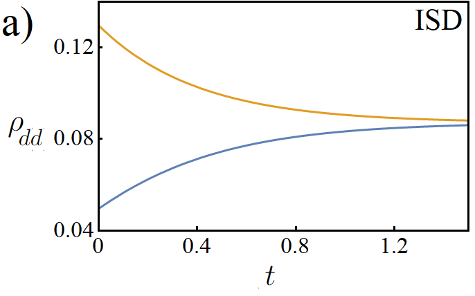
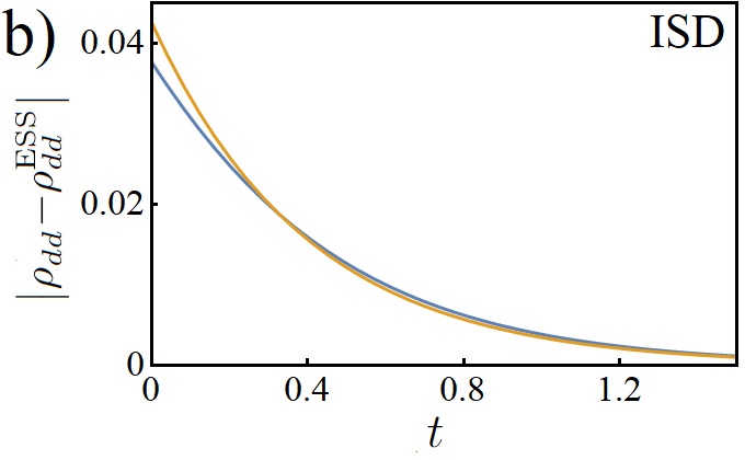
Figure 6: On crossing points in the time domain. (a): Time evolution of $\rho_{d,d}^{I}(t)$ (blue) and $\rho_{d,d}^{II}(t)$ (yellow curve) for the ISD model, using the parameters in Fig. 5 with $\mu_{L}^{I}=2.5$ and $\mu_{R}^{I}=0.1$. (b): Time evolution of $\left|\rho_{d,d}^{I}(t)-\rho_{d,d}^{\rm ESS}\right|$ (blue) and $\left|\rho_{d,d}^{II}(t)-\rho_{d,d}^{\rm ESS}\right|$ (yellow) for the ISD model, using again the parameters in panel (a). (c): Time evolution of $\rho_{2,2}^{I}(t)$ (blue) and $\rho_{2,2}^{II}(t)$ (yellow) for the I2KM with $t_{h}=1$, $\epsilon_{1}=\epsilon_{2}=2$, $\Delta=0.1$, $U=0.25$, $\Gamma=0.1$, and $\theta=0$. The system is driven towards a final ESS with $\mu_{L}^{\rm ESS}=\mu_{R}^{\rm ESS}=2.4$ and $\beta_{L}^{\rm ESS}=\beta_{R}^{\rm ESS}=2.15$, starting from two different pre-quench configurations with the same parameters except for $\mu_{L}^{I}=\mu_{L}^{II}=1.5$, $\beta_{L}^{I}=1.3$, and $\beta_{L}^{II}=0.7$.

We observe from Fig. 5 that the occurrence or absence of the QME depends on the monitoring function that one employs. In particular, using either the populations, see panel (a), or the absolute values of the population deviations from their final values, see panel (c), gives different phase diagrams. Moreover, since here we do not have a phase transition like in the original work on the classical ME [1], the system reaches the final (N)ESS only after infinitely long time through an exponential decay [2]. In practice, the critical time $t^{*}$ at which the crossing takes place can then become very large. At the same time, the distance of the monitored observable from its (N)ESS value then becomes extremely small, beyond numerical or experimental precision. For this reason, it is important to compare panels (a,c) with a situation where one imposes a resolution limit on the distance measurement. Once this limit has been reached, the search for a crossing point is terminated. In Fig. 5(b,d), we use such a cut-off scheme in order to implement this consideration. Evidently, the resulting phase diagrams in panels (b,d) are substantially different from the corresponding ones in panels (a,c), which were obtained by assuming perfect resolution capabilities.

Next, in Fig. 6(a), we show the time evolution of $\rho_{d,d}^{I}(t)$ and $\rho_{d,d}^{II}(t)$ for the parameters in Fig. 5 with $\mu_{L}^{I}=2.5$ and $\mu_{R}^{I}=0.1$. No crossing point is detected at any finite time but, clearly, the two density matrix elements approach the equilibrium value from above (initial condition $II$) and below (initial condition $I$). However, by comparing the time dependence of $\left|\rho_{d,d}^{I}(t)-\rho_{d,d}^{\rm ESS}\right|$ and $\left|\rho_{d,d}^{II}(t)-\rho_{d,d}^{\rm ESS}\right|$, see Fig. 6(b), we find that a critical time $t^{*}$ exists after which $\rho_{d,d}^{II}(t>t^{*})$ is nearer to the final ESS value than $\rho_{d,d}^{I}(t>t^{*})$. Together with Fig. 5 and the corresponding discussion, those observations show that the existence of a crossing point is in general not a necessary condition for the QME to take place.

Let us next show an example where the existence of crossing points does not give a sufficient condition for the QME. In the presence of both Lindblad and Liouvillian time evolution, as is the case for the I2KM, an oscillatory behavior is observed in many quantities. For such models, many crossing points can emerge, while no true QME is detected from the envelope of the oscillatory functions (for these parameters). In fact, in Fig. 6(c), for the I2KM case, we show the time evolution of the population of the state $\lvert 2\rangle$, see Eqs. (M4) and (M5), after two different initial conditions. Note that this state is not an eigenvector of the Hamiltonian. Evidently, the oscillatory behavior leads to finite-time crossings which artificially suggest a QME while the envelopes show that one of the curves is actually always closer to the final (N)ESS value.

To summarize, finite-time crossings of density matrix elements [7, 8, 9] do not provide a reliable guide to the identification of the QME. Crossing points can emerge due to oscillatory behavior, or they can simply be absent because the density matrix elements, for different initial conditions, approach the (N)ESS from above and below, respectively. It is worth mentioning that the presence of a crossing point in a generic observable could be purely accidental, e.g., due to natural constraints that the system must satisfy. For populations, for example, we have $\sum_{i}\rho_{i,i}(t)=1$ due to state normalization. As acknowledged in Ref. [9], quantum correlations are of fundamental importance for the QME. However, density matrix elements do not provide a suitable observable in this context.

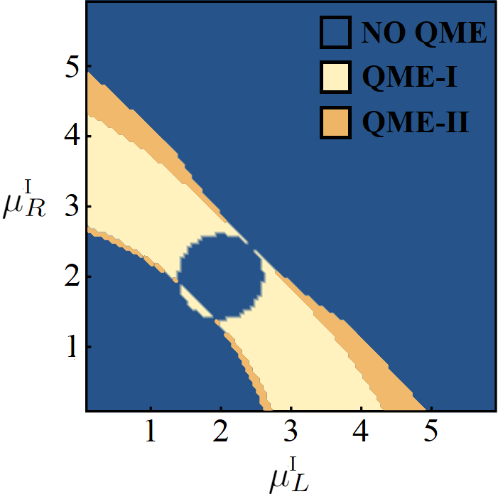
Figure 7: Phase diagram for the ISD model in the $\mu_{R}^{I}$-$\mu_{L}^{I}$ plane, obtained by using our trace distance protocol for the same parameters as in Fig. 5(c). Type-I and type-II QMEs (here dubbed QME-I and QME-II) have been identified as explained in the main text.

We next compare the phase diagram obtained from the crossing point procedure, see in particular Fig. 5(c), with the corresponding phase diagram for the ISD model computed from the trace distance protocol proposed in the main text. In Fig. 7, we show our results, which were obtained for the same parameters as in Fig. 5(c). It is rather obvious that the corresponding phase diagrams in Fig. 5(c) and Fig. 7 are very different. We conclude that, although it is legitimate to compare the time evolution of a generic system observable for different initial conditions, the existence of crossing points in the time evolution of density matrix elements is not one-by-one related to a QME. In our protocol, see Fig. 7 for the ISD model, the QME is instead detected through properly defined distance-from-equilibrium measures. This procedure is also able to distinguish type-I and type-II QMEs.

III II. Experimental quantities

In the main text, we introduced the trace distance ${\cal D}_{T}$ in Eq. (M2) as a proper distance measure for quantum states $\rho(t)$ from the final (N)ESS. The trace distance allows one to unambiguously detect the existence of the QME and its type. Moreover, it does not suffer from the limitations imposed by many other observables, as discussed in Sec. II. However, the trace distance is not an easily measurable quantity as it requires quantum state tomography. While this task is in principle possible, it is a challenge in practice. For this reason, we here compare its behavior with other quantities that can be experimentally measured with less effort. We focus on the I2KM introduced in the main text.

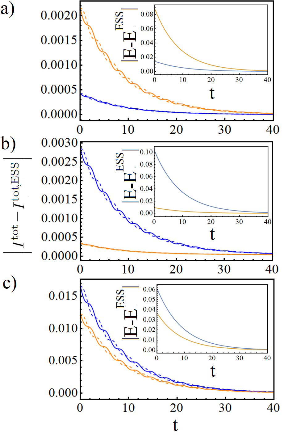
Figure 8: Currents ($I_{\lambda}^{\rm tot}$) and energy ($E$) in the time domain for the I2KM, where the indices $I$ vs $II$ refer to “close” vs “far” initial conditions. Main panels: Time evolution of current differences $\left|I_{\lambda}^{{\rm tot},I}(t)-I^{\rm tot,ESS}\right|$ (blue) and $\left|I_{\lambda}^{{\rm tot},II}(t)-I^{{\rm tot,ESS}}\right|$ (yellow), for the current flowing from the left ($\lambda=L$, solid) and right ($\lambda=R$, dashed) lead to the I2KM, respectively. We set $(T_{L,I}^{-1},\mu_{L,I})=(0.7,2.7)$ and $(T_{L,II}^{-1},\mu_{L,II})=(0.7,3)$. Others parameters are as in Fig. 3 of the main text, except for $\epsilon_{1}=\epsilon_{2}=\epsilon$ as specified below. (a): Case without QME, where $\epsilon=2.08$. (b): Type-I QME ($\epsilon=1.92$). (c): Type-II QME ($\epsilon=2$). Insets: Time evolution of energy differences $\left|E^{I}(t)-E^{\rm ESS}\right|$ (blue) and $\left|E^{II}(t)-E^{\rm ESS}\right|$ (yellow) to the final state for the two initial states, respectively.

In Fig. 8, we show the time evolution of the total current $I_{\lambda}^{\rm tot}(t)$ exchanged between lead $\lambda\in\{L,R\}$ and the I2KM, see Eq. (M10), and the time evolution of the energy $E(t)$ of the I2KM, see Eq. (M11). In the main panels, we plot the absolute value of the difference of the currents with respect to their final ESS values (which are independent of $\lambda$). When no QME is revealed by the trace distance protocol, the current of the “close” system (initial condition $I$) remains nearer to the ESS value for all times $t$ than the current of the “far” one (initial condition $II$), see the main panel in Fig. 8(a). On the other hand, when a type-I or a type-II QME is revealed by the trace distance protocol, cf. Fig. 4(a) in the main text, the distance between the time-dependent current and the ESS value of the “far” system remains always below the one for the “close” system, see the main panels in Fig. 8(b,c), respectively. However, no crossing point is detected in Fig. 8(c), and therefore the more elusive type-II QME cannot be distinguished from the type-I QME by simply analyzing the current. We conclude that quantum state tomography seems necessary to differentiate between type-I and type-II QMEs.

Very similar conclusions can also be drawn by analyzing the time-dependent energy of the I2KM system. For the three relevant cases (no QME, type-I QME, type-II QME), the corresponding curves for $\left|E(t)-E^{\rm ESS}\right|$ are shown in the respective insets of Fig. 8. Again, it is not possible to distinguish type-I and type-II QMEs based on this observable. However, one can distinguish the presence or absence of a QME in an unambiguous manner by measuring this observable.

In fact, the existence of a QME — leaving aside the classification into type-I or type-II cases — can already be established by measuring the currents $I_{\lambda}^{\rm tot}(t)$ or the energy $E(t)$ (relative to their final ESS values) at a time $t=0^{+}$ shortly after the parameter quench. The presence of a QME is characterized by the condition

$$\left|I_{\lambda}^{{\rm tot},I}(0^{+})-I^{\rm tot,ESS}\right|>\left|I_{\lambda}^{{\rm tot},II}(0^{+})-I^{\rm tot,ESS}\right|,$$ (20)

while otherwise no QME occurs. A similar condition applies to the total energy of the I2KM. The current between the two dots, $I_{1,2}$ in Eq. (M11), also allows one to draw the same conclusions in principle. However, $I_{1,2}$ is a strongly oscillatory function of time, since it also depends on the off-diagonal elements of $\rho(t)$. Nonetheless, its envelope, under initial condition $I$, always stays further away from (closer to) the final ESS value than for initial condition $II$ if the QME is present (absent). On the contrary, finite-time crossings of density-matrix based quantities like the von Neumann entropy or populations may result in misleading predictions, see Sec. II. Such pitfalls are avoided by following our protocol.

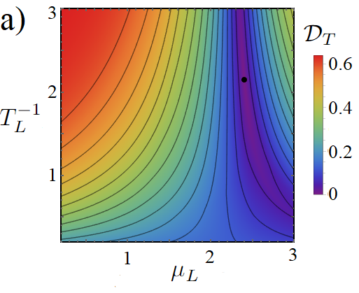
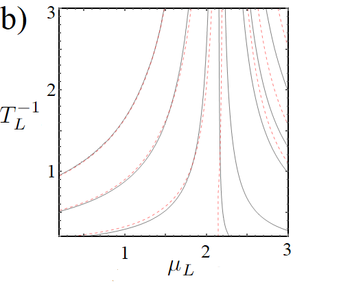
Figure 9: (a): Color-scale plot of the I2KM trace distance $\mathcal{D}_{T}(\rho(0))$ with respect to the final ESS (indicated by a black circle) in the $T_{L}^{-1}$-$\mu_{L}$ plane for different initial NESS configurations $(T^{-1}_{L},\mu_{L})$, where $(T^{-1}_{R},\mu_{R})$ is identical to the final ESS parameters, $T^{-1}_{\lambda,{\rm ESS}}=2.15$ and $\mu_{\lambda,{\rm ESS}}=2.4$ for $\lambda=L,R$. Other parameters are $t_{h}=1$, $\epsilon_{1}=\epsilon_{2}=2$, $\Delta=0.1$, $U=0.25$, $\Gamma=0.1$, and $\theta=0$. Thin black curves indicate $\mathcal{D}_{T}$-isolines. (b): Comparison between $\tau$-isolines [black solid lines, cf. Fig. 3 of the main text] and $\mathcal{D}_{T}$-isolines [red dashed lines, cf. panel (a)]. A deviation between these two isoline sets indicates a type-II QME.

If quantum state tomography is available, one can directly implement the trace distance protocol as discussed in the main text. In Fig. 9, we show that a comparison of the trace distance ${\cal D}_{T}$ between the close and far initial states and the final ESS with the respective values of the Euclidean distance ${\cal D}_{E}$ can directly reveal a type-II QME. Figure 3 in the main text shows how the absence or presence of the QME can be detected from the $\tau$-isolines in the bath parameter space. However, this information is not sufficient to discriminate between type-I and type-II QME. For that purpose, one needs to check the condition $\mathcal{D}_{T}(\rho_{f}(0))\gtrless\mathcal{D}_{T}(\rho_{c}(0))$ for the trace distance, see Fig. 9(a). Choosing, e.g., the “close” initial condition, we analyze the corresponding $\tau$-isoline and the $\mathcal{D}_{T}$-isoline crossing at that point. If there is a mismatch between the two isolines, see Fig. 9(b), a small region for the onset of the QME-II exists. In this region, the relaxation time starting with $\rho_{c}(0)$ is longer than if one starts from $\rho_{f}(0)$, but the trace distance for $\rho_{c}(0)$ is still smaller than for $\rho_{f}(0)$.

IV III. Optimal working point

In this section, we point out an interesting behavior that, albeit not directly connected with the QME, could play an important role in systems with complex geometries and in experiments. As observed in previous works [22, 24], when an interacting one-dimensional electronic chain is connected to two reservoirs, an optimal working point emerges through a change in the monotonicity of the NESS current as a function of the coupling between the chain and the reservoirs. The optimal working point is a consequence of the presence of two time scales in the dissipative quantum dynamics. First, there is an intrinsic time scale induced by the Hamiltonian. Second, there is a dissipative time scale set by the coupling strength $\Gamma$ to the baths.

For the I2KM, this effect appears through the geometric angle $\theta$ in Eq. (M9). For $\theta=0$, the system is connected in series with the two leads and the current $I_{1,2}$ between both dots is maximal. Indeed, an electron incoming from the left lead is forced to jump from dot $1$ to dot $2$ in order to reach the right lead. On the contrary, for $\theta=\pi/2$, the system is connected in parallel with the leads, and an electron can move from left to right by just populating one of the two dots. In this case, the classical vs quantum competition is reduced, with a qualitatively different dependence on $\Gamma$.

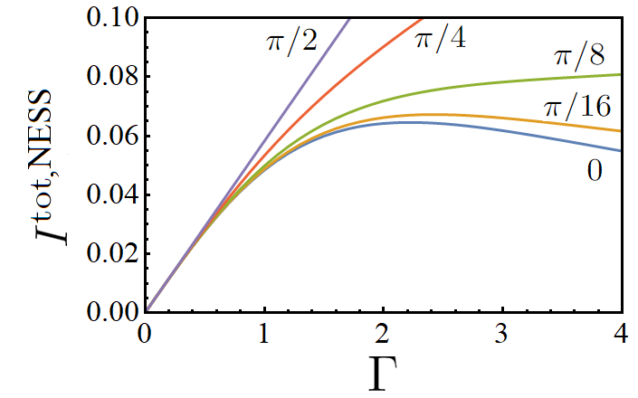
Figure 10: The NESS current $I^{\rm tot,NESS}$ (in units of $et_{h}/\hbar$) of the I2KM vs system-lead hybridization strength $\Gamma$, see Eq. (M10), for $t_{h}=1$, $\epsilon_{1}=\epsilon_{2}=2$, $\Delta=0.1$, and $U=0.25$. For arbitrary initial states, the system is driven towards a final NESS with $\mu_{L}^{\rm NESS}=2.4$, $\mu_{R}^{\rm NESS}=2.2$, $\beta_{L}^{\rm NESS}=2.15$, and $\beta_{R}^{\rm NESS}=1.15$. We study different geometric angles $\theta$ as specified near each curve.

In Fig. 10, the NESS current $I^{\rm tot,NESS}$, which neither depends on the chosen initial state nor on the lead index $\lambda$, is shown as a function of $\Gamma$ for different $\theta$. We observe that the largest current is obtained for $\theta=\pi/2$, while for $\theta=0$, the current has a maximum at a finite hybridization $\Gamma$, with a linear increase of the current for small $\Gamma$. An optimal working point thus emerges for $\theta=0$, or more generally for small values of $\theta\lesssim\pi/16$. In more complex geometries, such effects should be taken into consideration as they could affect not only the NESS current [22, 24] but also the relaxation time towards the final NESS configuration [25].

V IV. Sweet spot of I2KM

At the sweet parameter spot of the I2KM, $\Delta=t_{h}=1$ and $U=\epsilon_{1}=\epsilon_{2}=0$, two fine-tuned “poor man’s” Majorana bound states are localized on the first and second dot, respectively, without mutual overlap. This effectively cuts the I2KM into two halves, resulting in a vanishing current $I_{1,2}=0$. For $\theta=0$, the two leads are therefore dynamically decoupled. Here each dot relaxes to its own equilibrium state, which depends on the temperature and the chemical potential of the lead to which it is physically coupled. On the other hand, for $\theta=\pi/2$, a current can flow between both leads (but not between the dots), and the system effectively reduces to two independent dots coupled to both leads.

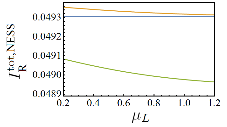
Figure 11: Sweet spot of the I2KM and effects of fine-tuned Majorana bound states. The NESS current $I_{R}^{\rm tot,NESS}$ between the I2KM and the right lead (in units of $et_{h}/\hbar$) is shown as function of $\mu_{L}=\mu_{L}^{\rm NESS}$ for $U=\epsilon_{1}=\epsilon_{2}=0,\,t_{h}=1,\,\Gamma=0.1,\,\mu_{R}^{\rm NESS}=2.4,\,\beta_{L}^{\rm NESS}=2.15$, and $\beta_{R}^{\rm NESS}=2.15$. The blue curve is for $\Delta=1$ and $\theta=0$, the yellow curve for $\Delta=1$ and $\theta=\pi/2$, and the green curve for $\Delta=1/2$ (away from the sweet spot) and $\theta=0$.

In Fig. 11, we consider the sweet spot regime and its vicinity. We show the NESS current $I_{R}^{\rm tot,NESS}$, see Eq. (M10), between the I2KM and the right lead as a function of $\mu_{L}=\mu_{L}^{\rm NESS}$ for fixed $\mu_{R}^{\rm NESS}$. For $\theta=0$, the current between the right dot and the right lead is not affected by the left dot, and thus stays constant for all $\mu_{L}$. At the same time, the non-zero NESS current is a signature for the poor man’s Majorana bound states which convert the incoming dissipative current into a supercurrent by means of Andreev reflection processes. For $\theta=\pi/2$, $I_{R}^{\rm tot,NESS}$ instead depends on $\mu_{L}$ due to a now finite transmission probability and the corresponding crossed Andreev reflection amplitude. Detuning the Hamiltonian parameters from the sweet spot condition, e.g., by setting $\Delta=1/2$ (see the green curve in Fig. 11), will destroy the poor man’s Majorana states. In such a case, the system is not anymore cut in two halves, and $I_{R}^{\rm tot,NESS}$ depends on $\mu_{L}$ even for $\theta=0$. At the same time, the current is reduced (compared to $\Delta=1$) due to the smaller Andreev reflection probability previously mediated by Majorana bound states.

Concerning the QME, the sweet spot regime of the I2KM behaves rather trivially when compared to the general case, reducing the problem to an effective single dot coupled to one ($\theta=0$) [2] or two ($\theta=\pi/2$) leads [7]. On the other hand, the transport properties of the I2KM, or in general of an $N$-site Kitaev chain (for $N=3$, see Ref. [21]), coupled to two leads in different geometries represent an interesting topic per se.

References

- Mpemba and Osborne [1969] E. B. Mpemba and D. G. Osborne, Cool?, Physics Education 4, 172 (1969).
- Lu and Raz [2017] Z. Lu and O. Raz, Nonequilibrium thermodynamics of the Markovian Mpemba effect and its inverse, Proceedings of the National Academy of Sciences 114, 5083 (2017).
- Murciano et al. [2024] S. Murciano, F. Ares, I. Klich, and P. Calabrese, Entanglement asymmetry and quantum Mpemba effect in the XY spin chain, Journal of Statistical Mechanics: Theory and Experiment 2024, 013103 (2024).
- Rylands et al. [2023] C. Rylands, K. Klobas, F. Ares, P. Calabrese, S. Murciano, and B. Bertini, Microscopic origin of the quantum Mpemba effect in integrable systems (2023), arXiv:2310.04419 [cond-mat.stat-mech] .
- Shapira et al. [2024] S. A. Shapira, Y. Shapira, J. Markov, G. Teza, N. Akerman, O. Raz, and R. Ozeri, The Mpemba effect demonstrated on a single trapped ion qubit (2024), arXiv:2401.05830 [quant-ph] .
- Joshi et al. [2024] L. K. Joshi, J. Franke, A. Rath, F. Ares, S. Murciano, F. Kranzl, R. Blatt, P. Zoller, B. Vermersch, P. Calabrese, C. F. Roos, and M. K. Joshi, Observing the quantum Mpemba effect in quantum simulations (2024), arXiv:2401.04270 [quant-ph] .
- Chatterjee et al. [2023a] A. K. Chatterjee, S. Takada, and H. Hayakawa, Quantum Mpemba Effect in a Quantum Dot with Reservoirs, Phys. Rev. Lett. 131, 080402 (2023a).
- Chatterjee et al. [2023b] A. K. Chatterjee, S. Takada, and H. Hayakawa, Multiple quantum Mpemba effect: exceptional points and oscillations (2023b), arXiv:2311.01347 [quant-ph] .
- Wang and Wang [2024] X. Wang and J. Wang, Mpemba effects in nonequilibrium open quantum systems (2024), arXiv:2401.14259 [quant-ph] .
- Strachan et al. [2024] D. J. Strachan, A. Purkayastha, and S. R. Clark, Non-Markovian Quantum Mpemba effect (2024), arXiv:2402.05756 [quant-ph] .
- Turkeshi et al. [2024] X. Turkeshi, P. Calabrese, and A. D. Luca, Quantum Mpemba Effect in Random Circuits (2024), arXiv:2405.14514 [quant-ph] .
- Nava and Fabrizio [2019] A. Nava and M. Fabrizio, Lindblad dissipative dynamics in the presence of phase coexistence, Phys. Rev. B 100, 125102 (2019).
- Holtzman and Raz [2022] R. Holtzman and O. Raz, Landau theory for the Mpemba effect through phase transitions, Communications Physics 5, 280 (2022).
- [14] See the Online Supplementary Material (SM), where we provide additional details on our derivations and results. .
- Nielsen and Chuang [2000] M. A. Nielsen and I. L. Chuang, Quantum Computation and Quantum Information (Cambridge University Press, Cambridge, UK, 2000).
- Wang and Schirmer [2009] X. Wang and S. G. Schirmer, Contractivity of the Hilbert-Schmidt distance under open-system dynamics, Phys. Rev. A 79, 052326 (2009).
- Leijnse and Flensberg [2012] M. Leijnse and K. Flensberg, Parity qubits and poor man’s Majorana bound states in double quantum dots, Phys. Rev. B 86, 134528 (2012).
- Tsintzis et al. [2024] A. Tsintzis, R. S. Souto, K. Flensberg, J. Danon, and M. Leijnse, Majorana Qubits and Non-Abelian Physics in Quantum Dot–Based Minimal Kitaev Chains, PRX Quantum 5, 010323 (2024).
- Samuelson et al. [2024] W. Samuelson, V. Svensson, and M. Leijnse, Minimal quantum dot based Kitaev chain with only local superconducting proximity effect, Phys. Rev. B 109, 035415 (2024).
- Dvir et al. [2023] T. Dvir, G. Wang, N. van Loo, C.-X. Liu, G. P. Mazur, A. Bordin, S. L. D. ten Haaf, J.-Y. Wang, D. van Driel, F. Zatelli, X. Li, F. K. Malinowski, S. Gazibegovic, G. Badawy, E. P. A. M. Bakkers, M. Wimmer, and L. P. Kouwenhoven, Realization of a minimal Kitaev chain in coupled quantum dots, Nature 614, 445 (2023).
- Bordin et al. [2024] A. Bordin, X. Li, D. van Driel, J. C. Wolff, Q. Wang, S. L. D. ten Haaf, G. Wang, N. van Loo, L. P. Kouwenhoven, and T. Dvir, Crossed Andreev Reflection and Elastic Cotunneling in Three Quantum Dots Coupled by Superconductors, Phys. Rev. Lett. 132, 056602 (2024).
- Benenti et al. [2009] G. Benenti, G. Casati, T. c. v. Prosen, D. Rossini, and M. Žnidarič, Charge and spin transport in strongly correlated one-dimensional quantum systems driven far from equilibrium, Phys. Rev. B 80, 035110 (2009).
- Bauer [2011] M. Bauer, Lindblad driving for nonequilibrium steady-state transport for noninteracting quantum impurity models (Bachelor Thesis, University of Munich, 2011).
- Nava et al. [2021] A. Nava, M. Rossi, and D. Giuliano, Lindblad equation approach to the determination of the optimal working point in nonequilibrium stationary states of an interacting electronic one-dimensional system: Application to the spinless Hubbard chain in the clean and in the weakly disordered limit, Phys. Rev. B 103, 115139 (2021).
- Artiaco et al. [2023] C. Artiaco, A. Nava, and M. Fabrizio, Wetting critical behavior in the quantum Ising model within the framework of Lindblad dissipative dynamics, Phys. Rev. B 107, 104201 (2023).
- Nazarov and Blanter [2009] Y. V. Nazarov and Y. M. Blanter, Quantum transport: Introduction to Nanoscience (Cambridge University Press, Cambridge, 2009).
- Nakajima et al. [2015] S. Nakajima, M. Taguchi, T. Kubo, and Y. Tokura, Interaction effect on adiabatic pump of charge and spin in quantum dot, Phys. Rev. B 92, 195420 (2015).
- Cao and Lu [2017] Y. Cao and J. Lu, Lindblad equation and its semiclassical limit of the Anderson-Holstein model, Journal of Mathematical Physics 58, 122105 (2017).
- Breuer and Petruccione [2007] H.-P. Breuer and F. Petruccione, The Theory of Open Quantum Systems (Oxford University Press, Oxford, 2007) p. 656.
- Woolf [2009] P. Woolf, Chemical Process Dynamics and Controls, Open textbook library (University of Michigan Engineering Controls Group, 2009).
- Lange and Timm [2021] S. Lange and C. Timm, Random-matrix theory for the Lindblad master equation, Chaos: An Interdisciplinary Journal of Nonlinear Science 31, 023101 (2021).
- Fernengel and Drossel [2020] B. Fernengel and B. Drossel, Bifurcations and chaos in nonlinear Lindblad equations, Journal of Physics A: Mathematical and Theoretical 53, 385701 (2020).
- Rose et al. [2016] D. C. Rose, K. Macieszczak, I. Lesanovsky, and J. P. Garrahan, Metastability in an open quantum Ising model, Phys. Rev. E 94, 052132 (2016).
- Nava et al. [2023a] A. Nava, G. Campagnano, P. Sodano, and D. Giuliano, Lindblad master equation approach to the topological phase transition in the disordered Su-Schrieffer-Heeger model, Phys. Rev. B 107, 035113 (2023a).
- Cinnirella et al. [2024] E. G. Cinnirella, A. Nava, G. Campagnano, and D. Giuliano, Fate of high winding number topological phases in the disordered extended Su-Schrieffer-Heeger model, Phys. Rev. B 109, 035114 (2024).
- Nava et al. [2023b] A. Nava, C. A. Perroni, R. Egger, L. Lepori, and D. Giuliano, Lindblad master equation approach to the dissipative quench dynamics of planar superconductors, Phys. Rev. B 108, 245129 (2023b).
- Nava et al. [2024] A. Nava, C. A. Perroni, R. Egger, L. Lepori, and D. Giuliano, Dissipation-driven dynamical topological phase transitions in two-dimensional superconductors, Phys. Rev. B 109, L041107 (2024).