On transience of $M/G/\infty$ queues

Abstract

We consider an $M/G/\infty$ queue with infinite expected service time. We then provide the transience/recurrence classification of the states (the system is said to be at state $n$ if there are $n$ customers being served), observing also that here (unlike e.g. irreducible Markov chains) it is possible for recurrent and transient states to coexist.
Keywords: transience, recurrence, service time, heavy tails
AMS 2020 subject classifications: 60K25, 60G55

In this note we consider a classical $M/G/\infty$ queue (see e.g. [1]): the customers arrive according to a Poisson process with rate $\lambda$; upon arrival, a customer immediately enters to service, and the service times are i.i.d. (nonnegative) random variables with some general distribution. For notational convenience, let $S$ be a generic random variable with that distribution. We also assume that at time $0$ there are no customers being served. Let us denote by $Y_{t}$ the number of customers in the system at time $t$, which we also refer to as the state of the system at time $t$; note that, in general, $Y$ is not a Markov process.

We are mainly interested in the situation where the system is unstable, i.e., when ${\mathbb{E}}S=\infty$. In this situation, in principle, our intuition tells us that the system can be transient (in the sense $Y_{t}\to\infty$ a.s.) or recurrent (i.e., all states are visited infinitely often a.s.). However, it turns out that, for this model, the complete picture is more complicated:

Theorem 1.

Define

$$k_{0}=\min\Big{\{}k\in{\mathbb{Z}}_{+}:\int_{0}^{\infty}\big{(}{\mathbb{E}}(S\wedge t)\big{)}^{k}\exp\big{(}-\lambda{\mathbb{E}}(S\wedge t)\big{)}\,dt=\infty\Big{\}}$$ (1)

(with the convention $\min\emptyset=+\infty$). Then

$$\liminf_{t\to\infty}Y_{t}=k_{0}\quad\text{a.s.}.$$ (2)

In particular, if

$$\int_{0}^{\infty}\big{(}{\mathbb{E}}(S\wedge t)\big{)}^{k}\exp\big{(}-\lambda{\mathbb{E}}(S\wedge t)\big{)}\,dt<\infty\qquad\text{ for all }k\geq 0,$$ (3)

then the system is transient; if

$$\int_{0}^{\infty}\exp\big{(}-\lambda{\mathbb{E}}(S\wedge t)\big{)}\,dt=\infty,$$ (4)

then the system is recurrent.

Proof.

We start with the following simple observation: for any $j$, $\{\liminf Y_{t}=j\}$ is a tail event, so it has probability $0$ or $1$. This implies that $\liminf Y_{t}$ is a.s. a constant (which may be equal to $+\infty$).

We use the following representation of the process (see Figure 1): consider a (two-dimensional) Poisson process in ${\mathbb{R}}_{+}^{2}$, with the intensity measure $\lambda\,dt\times dF_{S}(u)$, where $F_{S}(u)={\mathbb{P}}[S\leq u]$ is the distribution function of $S$. Then, a point $(t,u)$ of this Poisson process is interpreted in the following way: a customer arrived at time $t$ and the duration of its service will be $u$. Now, draw a (dotted) line in the SE direction from each point, as shown on the picture; as long as this line stays in ${\mathbb{R}}_{+}^{2}$, the corresponding customer is present in the system. If we draw a vertical line from $(t,0)$, then the number of dotted lines it intersects is equal to $Y_{t}$.

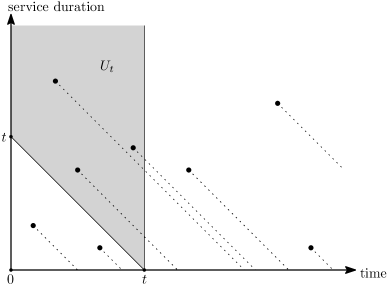
Figure 1: A Poisson representation of $M/G/\infty$. In this example, there are exactly three customers at time $t$.

Next, for $k\in{\mathbb{Z}}_{+}$ denote by

$$T_{k}:=\{t:Y_{t}=k\}$$

the set of time moments when the system has exactly $k$ customers, and let

$$U_{t}=\{(s,u)\in{\mathbb{R}}_{+}^{2}:s\in[0,t],u\geq t-s\}.$$

We note that $Y_{t}$ equals the number of points in $U_{t}$, which has Poisson distribution with mean

$$\int_{U_{t}}\lambda\,dt\,dF_{S}(u)=\lambda{\mathbb{E}}(S\wedge t).$$

Therefore, by Fubini’s theorem, we have

$${\mathbb{E}}|T_{k}|={\mathbb{E}}\int_{0}^{\infty}{\mathbf{1}\mkern-1.5mu}{\{Y_{t}=k\}}\,dt=\frac{\lambda^{k}}{k!}\int_{0}^{\infty}\big{(}{\mathbb{E}}(S\wedge t)\big{)}^{k}\exp\big{(}-\lambda{\mathbb{E}}(S\wedge t)\big{)}\,dt.$$ (5)

Now, assume that ${\mathbb{E}}|T_{k}|<\infty$ for some $k\geq 0$; this automatically implies that ${\mathbb{E}}|T_{\ell}|<\infty$ for $0\leq\ell\leq k$. This means that $|T_{0}|,\ldots,|T_{k}|$ are a.s. finite, and let us show that $T_{0},\ldots,T_{k}$ have to be a.s. bounded (this is a small technical issue that we have to resolve because we are considering continuous time). Probably, the cleanest way to see this is the following: first, notice that, in fact, $T_{0}$ is a union of intervals of random i.i.d. (with Exp($\lambda$) distribution) lengths, because each time when the system becomes empty, it will remain so till the arrival of the next customer. Therefore, $|T_{0}|<\infty$ clearly means that $\sup T_{0}\leq K_{0}$ for some (random) $K_{0}$. Now, after $K_{0}$ there are no $1\to 0$ transitions anymore, so the remaining part of $T_{1}$ again becomes a union of such intervals, meaning that it should be bounded as well; we then repeat this reasoning a suitable number of times to finally obtain that $T_{k}$ must be a.s. bounded. This implies that $\liminf_{t\to\infty}Y_{t}\geq k_{0}$ a.s..

Next, assume that $\{0,\ldots,k\}$ is a transient set, in the sense that $\liminf_{t\to\infty}Y_{t}\geq k+1$ a.s.. We then can choose a sufficiently large $h>0$ in such a way that

$${\mathbb{P}}\big{[}Y_{t}\geq k+1\text{ for all }t\geq h\big{]}\geq\frac{1}{2}.$$

Then, a simple coin-tossing argument together with the fact that an initially nonempty system (i.e., with some customers being served) dominates an initially empty system show that $|T_{k}|$ (in fact, $|T_{0}|+\cdots+|T_{k}|$) is dominated by $h\times\mathrm{Geom}_{0}\left({\frac{1}{2}}\right)$ random variable and therefore has a finite expectation. This shows that we have $\liminf_{t\to\infty}Y_{t}\leq k_{0}$ a.s. (because otherwise, in the situation when $k_{0}<\infty$, we would have ${\mathbb{E}}|T_{k_{0}}|<\infty$, which, by definition, is not the case). This concludes the proof of Theorem 1. ∎

Regarding this result, we may observe that, in most situations one would have $k_{0}=0$ or $+\infty$; this is because convergence of such integrals is usually determined by what is in the exponent. Still, it is not difficult to construct “strange examples” with $0<k_{0}<\infty$, i.e., where the process will visit $\{0,\ldots,k_{0}-1\}$ only finitely many times, but will hit every $k\geq k_{0}$ infinitely often a.s. (a behaviour one cannot have with irreducible Markov chains). For instance, take a service time distribution such that $1-F_{S}(u)=\frac{1}{u}+\frac{k_{0}+1}{u\ln u}$ for large enough $u$. Then it is elementary to obtain that $k_{0}$ is $k_{0}$.

References

- [1] G.F. Newell (1966) The queue. SIAM J. Appl. Math. 14 (1), 86–88.