Solving Poisson Equations using Neural Walk-on-Spheres

Abstract

We propose Neural Walk-on-Spheres (NWoS), a novel neural PDE solver for the efficient solution of high-dimensional Poisson equations. Leveraging stochastic representations and Walk-on-Spheres methods, we develop novel losses for neural networks based on the recursive solution of Poisson equations on spheres inside the domain. The resulting method is highly parallelizable and does not require spatial gradients for the loss. We provide a comprehensive comparison against competing methods based on PINNs, the Deep Ritz method, and (backward) stochastic differential equations. In several challenging, high-dimensional numerical examples, we demonstrate the superiority of NWoS in accuracy, speed, and computational costs. Compared to commonly used PINNs, our approach can reduce memory usage and errors by orders of magnitude. Furthermore, we apply NWoS to problems in PDE-constrained optimization and molecular dynamics to show its efficiency in practical applications.

1 Introduction

Partial Differential Equations (PDE) are foundational to our modern scientific understanding in a wide range of domains. While decades of research have been devoted to this topic, numerical methods to solve PDEs remain expensive for many PDEs. In recent years, deep learning has helped to accelerate the solution of PDEs (Azzizadenesheli et al., 2023; Zhang et al., 2023b; Cuomo et al., 2022) as well as tackle PDEs, which had been entirely out of range for classical methods (Han et al., 2018; Scherbela et al., 2022; Nüsken & Richter, 2021b).

Among the biggest challenges for classical numerical PDE solvers are complex geometries and high dimensions. In particular, grid-based methods, such as finite-element, finite-volume, or finite-difference methods, scale exponentially in the underlying dimension. On the other hand, deep learning approaches have been shown to overcome this so-called curse of dimensionality (De Ryck & Mishra, 2022; Duan et al., 2021; Berner et al., 2020b). Corresponding algorithms are typically based on Monte Carlo (MC) approximations of variational formulations of PDEs.

In this work, we focus on high-dimensional Poisson equations on general domains. We note that the accurate numerical solution of such types of PDEs is crucial for a large variety of areas. For instance, Poisson equations are prominent in geometry processing (Sawhney & Crane, 2020), as well as many areas of theoretical physics, e.g., electrostatics and quantum mechanics (Bahrami et al., 2014). In high dimensions, they govern important quantities in molecular dynamics, such as likely transition pathways and transition rates between regions or conformations of interest (Vanden-Eijnden et al., 2006; Lu & Nolen, 2015).

Several deep learning methods are amendable to the numerical solution of Poisson equations. This includes physics-informed neural networks (PINNs) or Deep Galerkin methods (Raissi et al., 2019; Sirignano & Spiliopoulos, 2018), the Deep Ritz method (E et al., 2017), as well as approaches based on (backward) stochastic differential equations (Han et al., 2017; Nüsken & Richter, 2021a; Han et al., 2020). However, previous methods suffer from unnecessarily high computational costs, bias, or instabilities, see Section 3.

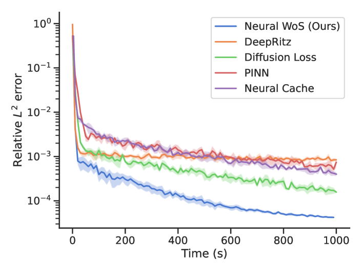
Figure 1: Convergence of the relative $L^{2}$-error when solving the 10$d$ Laplace equation in Section 5 using our considered methods.

Walk-on-Spheres (WoS):

To overcome the above challenges, we propose a novel approach based on so-called Walk-on-Spheres (WoS) methods (Muller, 1956). The WoS method is a Monte Carlo method specifically tailored toward Poisson equations by rewriting their solutions as an expectation over Brownian motions stopped at the boundary of the domain. Simulating the Brownian motion using time-discretizations either is slow or introduces bias (depending on the chosen time step). Leveraging the isotropy of Brownian motion, WoS accelerates this process by iteratively sampling from spheres around the current position until reaching the boundary, see Figure 2.

However, as with all Monte Carlo methods, WoS can only obtain pointwise estimates and suffers from slow convergence w.r.t. the number of trajectories. In particular, every sufficiently accurate estimate of the solution on a single point takes a considerable amount of time. This is prohibitive if many solution evaluations are needed sequentially, e.g., in PDE-constrained optimization problems.

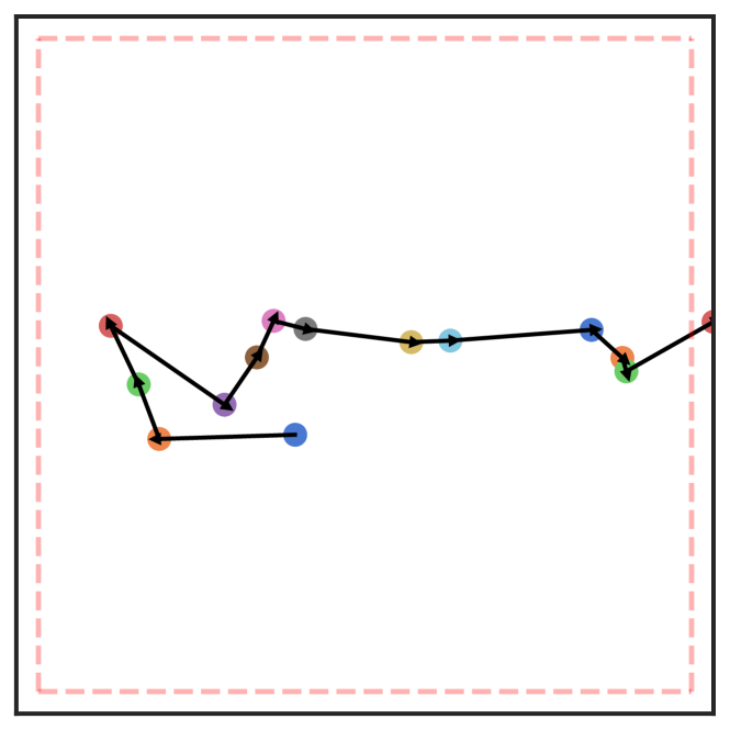
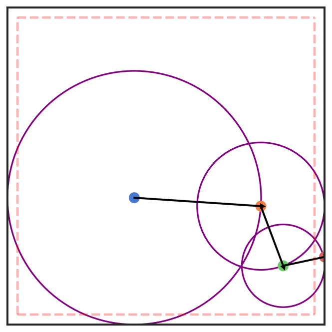
Figure 2: Left: Time-discretization of the solution $X^{\xi}$ to the SDE in (7) with stopping time $\tau(\Omega,\xi)$ in (8) for the domain $\Omega=[0,1]^{2}$.
Right: Realization of the Walk-on-Spheres algorithm in Section 4.

Our approach (NWoS):

We develop Neural Walk-on-Spheres (NWoS), a version of WoS that can be combined with neural networks to learn the solution to (parametric families of) Poisson equations on the whole domain. Our method amortizes the cost of WoS during training so that the solution, and its gradients, can be evaluated in fractions of seconds afterward (and at arbitrary points in the domain). In particular, in order to obtain accuracy $\varepsilon$, the standard WoS method incurs a cost of $\mathcal{O}(\varepsilon^{-2})$ trajectories for the evaluation of the solution while NWoS has a reduced cost of a single $\mathcal{O}(1)$ forward-pass of our model.

Using the partially trained model as an estimator, we can limit the number of simulations and WoS steps for training without introducing high bias or variance. The resulting objective is more efficient and scalable than competing methods, without the need to balance penalty terms for the boundary condition or compute spatial derivatives (Table 1). In particular, we demonstrate a significant reduction of GPU memory usage in comparison to PINNs (Figure 3) and up to orders of magnitude better performance for a given time and compute budget (Figure 1).

Our contributions can be summarized as follows:

• We analyze previous neural PDE solver and their shortcomings when applied to high-dimensional elliptic PDEs, such as Poisson equations (Section 3).

• We devise novel variational formulations for the solution of Poisson equations based on WoS methods and provide corresponding theoretical guarantees and efficient implementations (Section 4).

• We compare against previous approaches on a series of benchmarks and demonstrate significant improvements in terms of accuracy, speed, and scalability (Section 5).

Table 1: Comparison of neural PDE solver for Poisson equations. #Derivatives, #Loss terms, and Cost denote the order of spatial derivatives, the number of terms required in the loss function, and the computational cost for one gradient step. Propagation speed describes how quickly boundary information can propagate to the interior of the domain, see Section 3 for details.

Method	#Derivatives	#Loss	Cost	Propagation
		terms		speed
PINN	$2$	$2$	medium	slow
Deep Ritz	$1$	$2$	low	slow
Feynman-Kac	$0$	$1$	high	fast
BSDE	$1$	$1$	high	fast
Diffusion loss	$1$	$2$	medium	medium
NWoS (ours)	$\mathbf{0}$	$\mathbf{1}$	low	fast

Figure 3: Peak GPU memory usage of different methods during training with batch size $512$ for the Poisson equation in Section 5 in different dimensions $d$.

2 Related works

Neural PDE solver:

We provide an in-depth comparison to competing deep learning approaches to solve elliptic PDEs in Section 3. These include physics-informed neural networks (PINNs) (Raissi et al., 2019; Sirignano & Spiliopoulos, 2018), the Deep Ritz method (Jin et al., 2017), and the diffusion loss (Nüsken & Richter, 2021a), see also Table 1. The diffusion loss can be viewed as an interpolation between PINNs and losses based on backward SDEs (BSDEs) (Han et al., 2017; E et al., 2017; Beck et al., 2019). Methods based on BSDEs and the Feynman-Kac formula (Beck et al., 2018; Berner et al., 2020a; Richter & Berner, 2022) have been investigated for the solution of parabolic PDEs, where the SDE is stopped at a given terminal time. Due to costly simulation times, they cannot be applied efficiently to elliptic problems. To combat this issue, we draw inspiration from Walk-on-Spheres methods.

Monte Carlo (MC) methods:

Since grid-based methods cannot tackle high-dimensional PDEs, MC methods are typically used. For Poisson equations, the WoS method has been developed by Muller (1956) and has since been successfully used in various scientific settings (Sabelfeld, 2017; Juba et al., 2016; Bossy et al., 2010) as well as recently in computer graphics (Qi et al., 2022; Sawhney et al., 2022). In the latter domain, caches based on boundary values (Miller et al., 2023) and neural networks (Li et al., 2023) have been proposed to estimate the PDE solution across the domain and accelerate convergence. Our objective can be scaled to high-dimensional parametric PDEs and guarantees that its minimizer approximates the solution on the whole domain. We refer to Hermann et al. (2020); Beznea et al. (2022) for related neural network approximation results.

3 Neural PDE Solver for Elliptic PDEs

We start by defining our problem and describing previous deep learning methods for its solution. Our goal is to approximate the solution $u\in C(\Omega)$ to elliptic PDEs with Dirichlet boundary conditions of the form

$$\begin{cases}\mathcal{P}[u]=f,\quad&\text{on}\quad\Omega,\\ u=g,&\text{on}\quad\partial\Omega,\end{cases}$$ (1)

with differential operator

$$\mathcal{P}[u]\coloneqq\tfrac{1}{2}\mathrm{Tr}(\sigma\sigma^{\top}\mathrm{Hess}_{u})+\mu\cdot\nabla u.$$ (2)

In the above, $\Omega\subset\operatorname{\mathbb{R}}^{d}$ is an open, bounded, connected, and sufficiently regular domain, see, e.g., Baldi (2017); Karatzas & Shreve (2014); Schilling & Partzsch (2014) for suitable regularity assumptions. Note that the formulation in (1) includes the Poisson equation for $\mu=0$ and $\sigma=\sqrt{2}\mathrm{I}$, i.e.,

$$\begin{cases}\Delta u=f,\quad&\text{on}\quad\Omega,\\ u=g,&\text{on}\quad\partial\Omega.\end{cases}$$ (3)

In the following, we will summarize existing neural PDE solvers for these PDEs, see Table 1 for an overview. On a high level, they propose different variational formulations $\min_{v\in V}\,\mathcal{L}[v]$ with the property that the minimizer over a suitable function space $V\subset C(\Omega)$ is a solution $u$ to the PDE in (1). The space $V$ is then typically approximated by a set of neural networks with a given architecture, such that the minimization problem can be tackled using variants of stochastic gradient descent.

3.1 Strong and weak formulations of elliptic PDEs

Let us start with methods based on strong or weak formulations of the PDE in (1).

Physics-informed neural networks (PINNs):

In its basic form, the loss of PINNs (Raissi et al., 2019) or Deep Galerkin methods (Sirignano & Spiliopoulos, 2018), is given by

$$\mathcal{L}_{\mathrm{PINN}}[v]\coloneqq\operatorname*{\mathbbm{E}}\left[(\mathcal{P}[v](\xi)-f(\xi))^{2}\right]+\beta\mathcal{L}_{\mathrm{\mathrm{bnd}}}[v],$$ (4)

where

$$\mathcal{L}_{\mathrm{\mathrm{bnd}}}[v]\coloneqq\operatorname*{\mathbbm{E}}\left[(v(\zeta)-g(\zeta))^{2}\right].$$ (5)

In the above, $\beta\in(0,\infty)$ is a penalty parameter, and $\xi$ and $\zeta$ are suitable random variables distributed on $\Omega$ and $\partial\Omega$, respectively. While improved sampling methods have been investigated, see, e.g., Tang et al. (2023); Chen et al. (2023), the default choice is to pick uniform distributions. The expectations are then approximated with standard MC or quasi-MC methods based on a suitable set of samples.

By minimizing the point-wise residual of the PDE, PINNs have gained popularity as a universal and simple method. However, PINNs are sensitive to hyperparameter choices, such as $\beta$, and suffer from training instabilities or high variance (Wang et al., 2021; Krishnapriyan et al., 2021; Nüsken & Richter, 2021b). Moreover, the objective in (4) requires the evaluation of the derivatives appearing in $\mathcal{P}[v]$. While this can be done exactly using automatic differentiation, it leads to high computational costs, see Figure 3.

Deep Ritz method:

For the Poisson equation in (3), one can avoid this cost by leveraging weak variational formulations, see, e.g., Evans (2010). Rather than directly optimizing the regression loss in (4), the Deep Ritz method (E et al., 2017) proposes to minimize the objective

$$\mathcal{L}_{\mathrm{Ritz}}[v]\coloneqq\operatorname*{\mathbbm{E}}\left[\frac{\|\nabla v(\xi)\|^{2}}{2}-f(\xi)v(\xi)\right]+\beta\mathcal{L}_{\mathrm{\mathrm{bnd}}}[v].$$ (6)

Under suitable assumptions, the minimizer again corresponds to the solution to the PDE in (3). The objective only requires computing the gradient $\nabla v$ instead of the Laplacian $\Delta v$. Using backward mode automatic differentiation, this reduces the number of backward passes from $d+1$ to one, see also the reduced cost in Figure 3. Moreover, we note that the loss in (6) allows for weak solutions that are not twice differentiable. We refer to Chen et al. (2020), for an extensive comparison of the Deep Ritz method to PINNs for elliptic PDEs with different boundary conditions.

Finally, we mention that both methods suffer from the fact that the interior losses only consider local, pointwise information at samples $x\in\Omega$. At the beginning of training, the interior loss might thus not be meaningful. Specifically, the boundary condition $g$ first needs to be learned via the boundary loss $\mathcal{L}_{\mathrm{bnd}}$, and then propagate from the boundary $\partial\Omega$ to interior points $x$ via the local interior loss. There exist some heuristics to mitigate this issue by, e.g., progressively learning the solution, see Penwarden et al. (2023) for an overview. The next section describes more principled ways of including boundary information in the loss and directly informing the interior points of the boundary condition.

3.2 Stochastic formulations of elliptic PDEs

From weak solutions, we will now proceed to stochastic representations of elliptic PDEs in (1). To this end, consider the solution $X^{\xi}$ to the stochastic differential equation

$$\mathrm{d}X^{\xi}_{t}=\mu(X^{\xi}_{t})\,\mathrm{d}t+\sigma(X^{\xi}_{t})\,\mathrm{d}W_{t},\quad X^{\xi}_{0}=\xi,$$ (7)

where $W$ is a standard $d$-dimensional Brownian motion. Moreover, we define the stopping time $\tau$ as the first exit time of the stochastic process $X^{\xi}$ from the domain $\Omega$, i.e.,

$$\tau=\tau(\Omega,\xi)\coloneqq\inf\{t\in[0,\infty)\colon X_{t}^{\xi}\notin\Omega\}.$$ (8)

An application of Itô’s lemma to the process $u(X^{\xi}_{t\wedge\tau})$ shows that we almost surely have that

$$u(X^{\xi}_{\tau})=u(X^{\xi}_{0})+\int_{0}^{\tau}\mathcal{P}[u](X^{\xi}_{t})\,\mathrm{d}t+S^{u}_{\tau},$$ (9)

where $S_{\tau}^{u}$ is the stochastic integral

$$S_{\tau}^{u}\coloneqq\int_{0}^{\tau}(\sigma^{\top}\nabla u)(X^{\xi}_{t})\cdot\mathrm{d}W_{t}.$$ (10)

Using the fact that $X^{\xi}_{0}=\xi$ and assuming that $u$ solves the elliptic PDE in (1), we arrive at the formula

$$g(X^{\xi}_{\tau})=u(\xi)+F_{\tau}^{\xi}+S_{\tau}^{u},$$ (11)

where we used the abbreviation

$$F_{\tau}^{\xi}\coloneqq\int_{0}^{\tau}f(X^{\xi}_{t})\,\mathrm{d}t.$$ (12)

Since the stochastic integral $S^{\tau}_{u}$ has zero expectation, see, e.g., Baldi (2017, Theorem 10.2), we can rewrite (11) as a stochastic representation, i.e.,

$$u(x)=\operatorname*{\mathbbm{E}}\left[g(X^{\xi}_{\tau})-F_{\tau}^{\xi}\big{|}\xi=x\right],$$ (13)

which goes back to Kakutani’s Theorem (Kakutani, 1944) and is a special case of the Feynman-Kac formula.

While the representation in (13) leads to MC methods for the pointwise approximation of $u$ at a given point $x\in\Omega$, it also allows us to derive variational formulation for learning $u$ on the whole domain $\Omega$. Based on the above results, we can derive the following three losses.

Feynman-Kac loss:

The Feynman-Kac loss is given by

$$\mathcal{L}_{\mathrm{FK}}[v]\coloneqq\operatorname*{\mathbbm{E}}\Big{[}\big{(}v(\xi)-g(X^{\xi}_{\tau})+F_{\tau}^{\xi}\big{)}^{2}\Big{]}$$ (14)

and follows from the fact that the solution to a quadratic regression problem as in (14) is given by the conditional expectation in (13). Notably, this variational formulation does neither require a derivative of the function $v$ nor an extra boundary loss $\mathcal{L}_{\mathrm{bnd}}$.

BSDE loss:

Since the formula in (11) holds if and only if $u$ solves the PDE in (1), we can derive the BSDE loss

$$\mathcal{L}_{\mathrm{BSDE}}[v]\coloneqq\operatorname*{\mathbbm{E}}\Big{[}\big{(}v(\xi)-g(X^{\xi}_{\tau})+F_{\tau}^{\xi}+S_{\tau}^{v}\big{)}^{2}\Big{]}.$$ (15)

Compared to the Feynman-Kac loss in (14), the BSDE loss requires computing the gradient of $v$ at every time-discretization of the SDE $X^{\xi}$ in order to compute $S_{\tau}^{v}$. However, due to (11), $S_{\tau}^{v}$ acts as a control variates and causes the variance of the MC estimator of (15) to vanish at the optimum, see Richter & Berner (2022) for details.

For the previous two losses, boundary information is directly propagated along the trajectory of the SDE $X^{\xi}$ to the interior. However, simulating a batch of realizations of the SDE until they reach the boundary $\partial\Omega$, i.e., until the stopping time $\tau$, can incur prohibitively high costs.

Diffusion loss:

The diffusion loss (Nüsken & Richter, 2021a) circumvents long simulation times by stopping the SDE at $s=\tau\wedge T$, i.e., at the minimum of a prescribed time $T\in(0,\infty)$ and the stopping time $\tau$. Since the trajectories might not reach the boundary, the loss is supplemented with a boundary loss. This yields the variational formulation

$$\mathcal{L}_{\mathrm{Diff}}[v]\coloneqq\operatorname*{\mathbbm{E}}\big{[}\big{(}v(\xi)-v(X^{\xi}_{s})+F^{\xi}_{s}+S_{s}^{v}\big{)}^{2}\big{]}+\beta\mathcal{L}_{\mathrm{bnd}}[v].$$ (16)

Note that this can be viewed as an interpolation between the BSDE loss (for $s\to\infty$) and the PINN loss (for $s\to 0$ and rescaling by $s^{-2}$). In the same way, it also balances the advantages and disadvantages of both losses, see also Table 1.

4 Neural Walk-on-Spheres (NWoS) Method

In this section, we will present a more efficient way of simulating the SDE trajectories for the case of Poisson-type PDEs as in (3). Our loss is based on the FK loss in (14), which does not require the computation of any spatial derivatives of the neural network $v$. However, we reduce the number of steps for simulating the process $X^{\xi}$ while still reaching the boundary (different from the diffusion loss).

4.1 Recursion of elliptic PDEs on sub-domains

First, we outline how to cast the solution of the PDE in (1) into nested subproblems of solving elliptic PDEs on subdomains. Specifically, let $\Omega_{0}\subset\Omega$ be an open sub-domain containing $\xi_{0}\coloneqq\xi$ and let $\tau_{0}\coloneqq\tau(\Omega_{0},\xi)$ be the corresponding stopping time, defined as in (8). Analogously to (13), we obtain that

$$u(\xi)=\operatorname*{\mathbbm{E}}\left[u(X^{\xi}_{\tau_{0}})-F^{\xi}_{\tau_{0}}\big{|}\xi\right].$$ (17)

Note that this is a recursive definition since the solution $u$ to the PDE in (1) appears again in the expectation. To resolve the recurrence, we define the random variable $\xi_{1}\sim X^{\xi}_{\tau_{0}}$ and choose another open sub-domain $\Omega_{1}\subset\Omega$ containing $\xi_{1}$. Considering the stopping time $\tau_{1}\coloneqq\tau(\Omega_{1},\xi_{1})$, we can calculate the value of $u$ appearing in the inner expectation

$$u(X^{\xi}_{\tau_{0}})\sim u(\xi_{1})=\operatorname*{\mathbbm{E}}\left[u(X^{\xi_{1}}_{\tau_{1}})-F_{\tau_{1}}^{\xi_{1}}\big{|}\xi_{1}\right]$$ (18)

We can now iterate this process for $k\in\mathbb{N}$ and combine the result with (17) to obtain

$$u(\xi)=\operatorname*{\mathbbm{E}}\Bigg{[}g(X^{\xi}_{\tau})-\sum_{k\geq 0}F^{\xi_{k}}_{\tau_{k}}\Bigg{|}\xi\Bigg{]}.$$ (19)

In the above, we used the strong Markov property of the SDE solution and the tower property of the conditional expectation, see also Hermann et al. (2020). This nested stochastic representation can be compared to the one in (13). The next section shows how this provides a practical algorithm that terminates in finitely many steps.

4.2 Walk-on-Spheres

We tackle the problem of solving the Poisson equation in (3), i.e., $\mu=0$ and $\sigma=\sqrt{2}\mathrm{I}$. Then, the SDE in (7) is just a scaled Brownian motion starting at $\xi$. Picking $\Omega_{k}\coloneqq B_{r_{k}}(\xi_{k})$ to be a ball of radius $r_{k}\in(0,\infty)$ around $\xi_{k}$ in the $k$-th step, the isotropy of Brownian motion ensures that

$$\xi_{k+1}\sim X^{\xi_{k}}_{\tau_{k}}\sim\mathcal{U}(\partial B_{r_{k}}(\xi_{k})).$$ (20)

In other words, we can just sample $\xi_{k+1}$ uniformly from a sphere of radius $r_{k}$ around the previous value $\xi_{k}$. To terminate after finitely many steps, we pick the maximal radius in each step, i.e.,

$$r_{k}\coloneqq\operatorname{dist}(\xi_{k},\partial\Omega),$$ (21)

and stop at step $\kappa$ when reaching an $\varepsilon$-shell, i.e., when $r_{\kappa}<\varepsilon$ for a prescribed $\varepsilon\in(0,\infty)$. This allows us to “walk” from sphere to sphere until (approximately) reaching the boundary, such that we can estimate the first term in (19). Specifically, the value $u(X^{\xi}_{\tau})$ in (19) is approximated by the boundary value $g(\bar{\xi}_{\kappa})$, where

$$\bar{\xi}_{\kappa}\coloneqq\operatorname*{arg\,min}_{x\in\partial\Omega}\|x-\xi_{\kappa}\|$$ (22)

is the projection to the boundary.

We note that the bias from introducing the stopping tolerance $\varepsilon$ can be estimated as $\mathcal{O}(\varepsilon)$ (Mascagni & Hwang, 2003). Moreover, for well-behaved, e.g., convex, domains $\Omega$, the average number of steps $\kappa$ behaves like $\mathcal{O}(\log(\varepsilon^{-1}))$ (Motoo, 1959; Binder & Braverman, 2012). This shows that $\varepsilon$ can be chosen sufficiently small without incurring too much additional computational cost. We note that this leads to much faster convergence than time-discretizations of the Brownian motion. In order to have a comparable bias, we would need to take steps of size $\mathcal{O}(\varepsilon)$, requiring $\Omega(\varepsilon^{-2})$ steps to converge.

4.3 Source term

To compute the second term in (19), we need to accumulate values of the form

$$v(z)\coloneqq\operatorname*{\mathbbm{E}}\left[-F^{z}_{\tau(B,z)}\right]$$ (23)

with a given ball $B=B_{r}(z)$. By (13), we observe that $v$ is the solution of a Poisson equation on the ball $B$ with zero Dirichlet boundary condition evaluated at $z\in\Omega$. We can thus use classical results by Boggio (1905), see also Gazzola et al. (2010), to write the solution in terms of Green’s functions. Specifically, we have that

$$v(z) =-|B_{r}(z)|\operatorname*{\mathbbm{E}}[f(\gamma)G_{r}(\gamma,z)],$$ (24)

where $\gamma\sim\mathcal{U}(B_{r}(z))$ and

$$G_{r}(y,z)\coloneqq\begin{cases}\frac{1}{2\pi}\log\frac{r}{\|y-z\|},&d=2,\\[3.99994pt] \frac{\Gamma(d/2-1)}{4\pi^{d/2}}\left(\|y-z\|^{2-d}-r^{2-d}\right),&d>2,\end{cases}$$ (25)

see Appendix A for further details. In practice, we can now approximate the expectation in (24) using an MC estimate.

4.4 Learning Problem

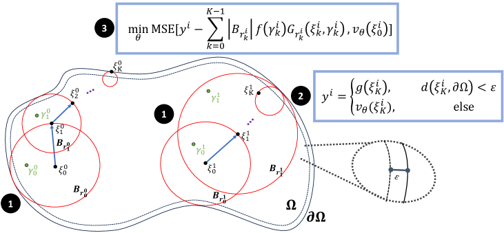
Figure 4: Neural Walk-on-Spheres (NWoS): Our algorithm for learning the solution to Poisson equations $\Delta u=f$ on $\Omega\subset\operatorname{\mathbb{R}}^{d}$ and $u|_{\partial\Omega}=g$. In each gradient descent step, we sample a batch of random points $(\xi_{0}^{i})_{i=1}^{m}$ in the domain $\Omega$ and simulate Brownian motions by iteratively sampling $\xi_{k}^{i}$ from spheres $B_{r^{i}_{k}}$ inscribed in the domain. To account for the source term $f$, we sample $\gamma_{k}^{i}\sim\mathcal{U}(B_{r^{i}_{k}})$ to compute an MC approximation $|B_{r^{i}_{k}}|f(\gamma_{k}^{i})G_{r_{k}^{i}}(\xi_{k}^{i},\gamma_{k}^{i})$ to the solution of the Poisson equation on the sphere $B_{r^{i}_{k}}$ using the Green’s function $G_{r_{k}^{i}}$ in Section 4.3. We stop after a fixed number of maximum steps $K$ and either evaluate our neural network $v_{\theta}$ or the boundary condition $g$ if we reach an $\varepsilon$-shell of $\partial\Omega$. If $v_{\theta}$ satisfies the PDE, the mean-value property implies that $v_{\theta}(\xi_{0}^{i})$ is approximated by the expected value of $y^{i}$ minus the accumulated source term contributions. We thus minimize the corresponding mean squared error over the parameters $\theta$ using gradient descent.

Based on the previous derivations, we can establish a variational formulation, where the minimizer is guaranteed to approximate the Poisson equation in (3) on the whole domain $\Omega$. Specifically, we define

$$\mathcal{L}_{\mathrm{NWoS}}[v]\coloneqq\operatorname*{\mathbbm{E}}\Big{[}\big{(}v(\xi)-\operatorname{WoS}(\xi)\big{)}^{2}\Big{]},$$ (26)

where the single-trajectory WoS method $\operatorname{WoS}(\xi)$ with random initial point $\xi$ is given by

$$\operatorname{WoS}(\xi)\coloneqq g(\bar{\xi}_{\kappa})-\sum_{k=0}^{\kappa-1}|B_{r_{k}}(\xi_{k})|f(\gamma_{k})G_{r_{k}}(\gamma_{k},\xi_{k}).$$ (27)

In the above, $\gamma_{k}\sim\mathcal{U}(B_{{r_{k}}}(\xi_{k}))$, and the random variables $\kappa$, $\xi_{k}$, $\bar{\xi}_{\kappa}$, and $r_{k}$ are defined as in Section 4.2. From the stochastic formulation of the solution in (19) and Proposition 3.5 in Hermann et al. (2020), it follows that the minimizer of (26), i.e., $x\mapsto\operatorname*{\mathbbm{E}}\big{[}\operatorname{WoS}(\xi)\big{|}\xi=x\big{]}$, approximates the solution $u$ in (3) in the uniform norm up to error $\mathcal{O}(\varepsilon)$, where $\varepsilon$ is the stopping tolerance, see Section 4.2. We also remark that, in theory, the loss requires only a single WoS trajectory per sample of $\xi$ since the minimizer of the regression problem in (26) averages out the noise.

Having established a learning problem, we can analyze both approximation and generalization errors. For the former, Hermann et al. (2020) and Beznea et al. (2022) bounded the size of neural networks $v_{\theta}$ to approximate the solution $u$ up to a given accuracy. In particular, the number of required parameters $\theta$ only scales polynomially in the dimension $d$ and the reciprocal accuracy, as long as the functions $f$, $g$, and $\operatorname{dist}(\cdot,\partial\Omega)$ can be efficiently approximated by neural networks.

One can then leverage results by Berner et al. (2020b) to show that also the generalization error does not underlie the curse of dimensionality when minimizing the empirical risk, i.e., an MC approximation of (26), over a suitable set of neural networks $v_{\theta}$. Specifically, the number of required samples of $\xi$ to guarantee that the empirical minimizer approximates the solution $u$ up to a given accuracy also scales only polynomially with dimension and accuracy.

4.5 Implementation

In this section, we discuss implementations for the loss $\mathcal{L}_{\mathrm{NWoS}}$ in (26) described in the previous section. We summarize our algorithm in Figure 4 and provide pseudocode for the vanilla version in Algorithm 1. In the following, we present strategies to trade-off accuracy and computational cost and to reduce the variance of MC estimators. We provide pseudocode for NWoS with these improvements in LABEL:alg:NWoS and LABEL:alg:wos_single in the appendix.

Table 2: Relative $L^{2}$-error (and standard deviations over $5$ independent runs) of our considered methods, estimated using MC integration on $10^{6}$ uniformly distributed (unseen) points in $\Omega$.

Method	Problem
	Laplace ($10d$)	Committor ($10d$)	Poisson Rect. ($10d$)	Poisson ($50d$)
PINN	$7.42e^{-4}\pm 1.84e^{-4}$	$4.10^{-3}\pm 1.11e^{-3}$	$1.35e^{-2}\pm 1.57e^{-3}$	$7.70e^{-3}\pm 2.25e^{-3}$
Deep Ritz	$8.43e^{-4}\pm 6.29e^{-5}$	$6.15e^{-3}\pm 5.30e^{-4}$	$1.06e^{-2}\pm 6.20e^{-4}$	$1.05e^{-3}\pm 1.70e^{-4}$
Diffusion loss	$1.57e^{-4}\pm 7.74e^{-6}$	$4.48e^{-2}\pm 6.93e^{-3}$	$9.69e^{-2}\pm 1.03e^{-2}$	$5.96e^{-4}\pm 1.06e^{-5}$
Neural Cache	$3.99^{-4}\pm 4.08e^{-5}$	$1.26e^{-3}\pm 5.82e^{-5}$	$4.98e^{-2}\pm 1.80e^{-2}$	$1.63e^{-2}\pm 1.42e^{-2}$
WoS	$1.08e^{-3}\pm 1.34e^{-6}$	$1.99e^{-3}\pm 9.79e^{-6}$	$2.32e^{-1}\pm 2.09e^{-1}$	$4.50e^{-3}\pm 7.38e^{-4}$
NWoS (ours)	$\mathbf{4.29e^{-5}\pm 2.02e^{-6}}$	$\mathbf{6.56e^{-4}\pm 2.42e^{-5}}$	$\mathbf{2.60e^{-3}\pm 9.99e^{-5}}$	$\mathbf{4.82e^{-4}\pm 1.32e^{-5}}$

WoS with maximum number of steps:

For sufficiently regular geometries, the probability of a walk taking more than $k$ steps is exponentially decaying in $k$ (Binder & Braverman, 2012). However, if a single walk in our batch needs significantly more steps, it slows down the overall training. We thus introduce a deterministic maximum number of steps $K\in\mathbb{N}$; see Beznea et al. (2022) for a corresponding error analysis. However, we do not want to introduce non-negligible bias by, e.g., just projecting to the closest point on the boundary.

Instead, we want to enforce the mean-value property on subdomains of $\Omega$ based on our recursion in Section 4.1. We thus propose to use the model $v$ instead of the boundary condition $g$ if the walk does not converge after $K$ steps, i.e., we define

$$y^{\xi,v}\coloneqq\begin{cases}v(\xi_{K}),&d(\xi_{K},\partial\Omega)>\varepsilon,\\ g(\bar{\xi}_{K}),&\textrm{else.}\end{cases}$$ (28)

We can then replace the second term in (26) by

$$\operatorname{WoS}(\xi,v)\coloneqq y^{\xi,v}-\sum_{k=0}^{K-1}|B_{r_{k}}(\xi_{k})|f(\gamma_{k})G_{r_{k}}(\gamma_{k},\xi_{k}).$$ (29)

This helps to reduce the bias when $d(\xi_{K},\partial\Omega)$ is non-negligible and leads to faster convergence assuming that we obtain increasingly good approximations $v_{\theta}\approx u$ during training of a neural network $v_{\theta}$. Our approach bears similarity to the diffusion loss, see Section 3; however, we do not need to use a time-discretization of the SDE.

Boundary Loss:

We find empirically that an additional boundary loss can improve the performance of our method. While theoretically not required, it can especially help for a smaller number $K$ of maximum steps (see the previous paragraph). In general, we thus sample a fraction of the points on the boundary $\partial\Omega$ and optimize

$$\mathcal{L}_{\mathrm{NWoS}}[v]+\beta\mathcal{L}_{\mathrm{\mathrm{bnd}}}[v],$$ (30)

where $\mathcal{L}_{\mathrm{\mathrm{bnd}}}$ is defined as in (5).

Variance-reduction:

While not necessarily needed for the objective in (26), we can still average multiple WoS trajectories $N\in\mathbb{N}$ per sample of $\xi$ to reduce the variance. This leads to the estimator

$$\!\!\widehat{\mathcal{L}}_{\mathrm{NWoS}}[v]\coloneqq\frac{1}{m}\left(\sum_{i=1}^{m}v(\xi^{i})-\frac{1}{N}\sum_{n=1}^{N}\operatorname{WoS}^{n}(\xi^{i})\right)\!,$$ (31)

where $\xi^{i}$ are i.i.d. samples of $\xi$ and $\operatorname{WoS}^{n}(\xi^{i})$ are i.i.d. samples of $\operatorname{WoS}(\xi^{i})$, i.e., $N$ trajectories with the same initial point $\xi^{i}$, see (26). Note that we vectorize the WoS simulations across both the initial points and the trajectories, making our NWoS method highly parallelizable and scalable to large batch sizes.

We further introduce control variates to reduce the variance of estimating $\operatorname{WoS}(x)$, where we focus on a fixed $x\in\Omega$ for ease of presentation. Control variates seek to reduce the variance by using an estimator of the form

$$\operatorname*{\mathbbm{E}}\left[\operatorname{WoS}(x)\right]\approx\operatorname*{\mathbbm{E}}[\delta]+\frac{1}{N}\sum_{n=1}^{N}\operatorname{WoS}^{n}(x)-\delta^{n},$$ (32)

where $\delta^{n}$ are i.i.d. samples of a random variable $\delta$ with known expectation.

Motivated by Sawhney & Crane (2020), we use an approximation of the first-order term of a Taylor series of $u$ in the direction of the first WoS step. We assume that $\nabla v_{\theta}$ provides an increasingly accurate approximation of the gradient $\nabla u$ during training and propose to use

$$\delta^{n}\coloneqq\nabla v_{\theta}(x)\cdot(\xi^{n}_{1}-x),$$ (33)

where $\xi^{n}_{1}$ is the first step of $\operatorname{WoS}^{n}(x)$. In particular, $\xi^{n}_{1}\sim\mathcal{U}(\partial B_{r_{1}}(x))$ and thus $\operatorname*{\mathbbm{E}}[\delta]=0$ holds for any function $v_{\theta}$.

While we need to compute the gradient $\nabla v_{\theta}(x)$ for the control variate, we mention that this operation can be detached from the computational graph. In particular, we do not need to compute the derivative of $\nabla v_{\theta}(x)$ w.r.t. the parameters $\theta$ as is necessary for PINNs, the Deep Ritz method, the diffusion loss, and the BSDE loss. In LABEL:app:ablation, we empirically show that the overhead of using the control variates is insignificant.

Buffer:

Motivated by Li et al. (2023), we can use a buffer to cache training points

$$\Big{(}\xi^{(i)},\frac{1}{N}\sum_{n=1}^{N}\mathrm{WoS}^{n}(\xi^{(i)})\Big{)}_{i=1}^{B}.$$ (34)

Since we only update the buffer after a given number of training steps $L\in\mathbb{N}$, this accelerates the training. Note that this is not possible for the other methods since they require evaluation of the current model or its gradients. In every buffer update, we average over additional trajectories, i.e., increase $N$ in (34), for a fraction of points to improve their accuracy. However, different from Li et al. (2023), we also evict a fraction of points from the buffer and replace them with WoS estimates on newly sampled points $\xi^{(i)}$ in the domain $\Omega$ to balance the diversity and accuracy of the training data in the buffer.

Remark 4.1.

The Neural Cache method by Li et al. (2023) uses a related approach to accelerate WoS methods for applications in computer graphics. However, their method never replaces any point $\xi^{(i)}$ in the buffer, i.e., only updates estimates in the buffer. We observed that the model is thus prone to overfitting on the points in the buffer, especially in high dimensions, preventing it from achieving high accuracies across the domain $\Omega$.

neural network $v_{\theta}$with initial parameters $\theta$, optimizer method $\operatorname{step}$for updating the parameters, number of iterations $T$, batch size $m$, source term $f$, boundary term $g$, stopping tolerance $\varepsilon$optimized parameters $\theta$$k\leftarrow 0,\dots,T$$x_{\Omega}\leftarrow\text{sample from }\xi^{\otimes m}$Sample points in $\Omega$$x\leftarrow x_{\Omega}$$r\leftarrow\operatorname{dist}(x,\partial\Omega)$Compute distances to $\partial\Omega$$r>\varepsilon$$\gamma\leftarrow\text{sample from }\mathcal{U}(B_{r}(x))$Estimate source $s\leftarrow s-|B_{r}(x)|f(\gamma)G_{r}(x,\gamma)$$u\leftarrow\text{sample from }\mathcal{U}(\partial B_{r}(x))$$x\leftarrow x+u$Walk to next points $r\leftarrow\operatorname{dist}(x,\partial\Omega)$Compute distances to $\partial\Omega$$x\leftarrow$project $x$to $\partial\Omega$Find closest points in $\partial\Omega$$y_{\Omega}\leftarrow s+g(x)$Estimate boundary $\widehat{\mathcal{L}}_{\mathrm{NWoS}}\leftarrow\operatorname{MSE}(v_{\theta}(x_{\Omega}),y_{\Omega})$NWoS loss $\theta\leftarrow\operatorname{step}\big{(}\gamma,\nabla_{\theta}\widehat{\mathcal{L}}_{\mathrm{NWoS}}\big{)}$SGD step

Algorithm 1 Training of vanilla NWoS method

5 Experiments

In this section, we compare the performance of NWoS, PINN, DeepRitz, Diffusion loss, and Neural Cache on various problems across dimensions from $10d$ to $50d$. We do not consider the FK and BSDE losses since they incur prohibitively long runtimes for simulating the SDEs with sufficient precision. To compare against the baselines, we consider benchmarks from the works proposing the Deep Ritz and diffusion losses (Jin et al., 2017; Nüsken & Richter, 2021a). For a fair comparison, we set a fixed runtime of $25d+750$ seconds and GPU memory budget of $2$GiB for training and ran a grid search over a series of hyperparameter configurations for each method. Then, we performed $5$ independent runs for the best configurations w.r.t. the relative $L^{2}$-error. More details on the hyperparameters and our implementations can be found in LABEL:app:implementation.

Laplace Equation:

The first PDE is a Laplace equation on a square domain given by

$$\textstyle f(x)=0,\quad g(x)=\sum_{i=0}^{d/2}x_{2i}x_{2i+1},\quad x\in\Omega=(0,1)^{d}.$$ (35)

To test our models, we compare against the analytic solution as $u(x)=\sum_{i=0}^{d/2}x_{2k}x_{2k+1}$. Following Jin et al. (2017), we consider the case $d=10$.

Poisson Equation:

Next, we consider the Poisson equation presented in Jin et al. (2017), i.e.,

$$\textstyle f(x)=2d,\quad g(x)=\sum_{i=1}^{d}x_{i}^{2},\quad x\in\Omega=(0,1)^{d},$$ (36)

with analytic solution $u(x)=\sum_{i=1}^{d}x_{i}^{2}$. We choose $d=50$ and present results with $d\in\{100,500\}$ in LABEL:app:additional_eval.

Poisson Equation with Rectangular Annulus:

We also consider a Poisson equation on a rectangular annulus $\Omega=(-1,1)^{d}\setminus[-c,c]^{d}$ with sinusoidal boundary condition and source term

$$g(x)=\frac{1}{d}\sum_{i=1}^{d}\sin(2\pi x_{i}),\quad f(x)=-\frac{4\pi^{2}}{d}\sum_{i=1}^{d}\sin(2\pi x_{i}).$$ (37)

We choose $c=0.25^{\frac{1}{d}}$ and $d=10$, and note that the analytic solution is given by $u(x)=\frac{1}{d}\sum_{i=1}^{d}\sin(2\pi x_{i})$.

Committor Function:

The fourth equation deals with committor functions from molecular dynamics. These functions specify likely transition pathways and transition rates between (potentially metastable) regions or conformations of interest (Vanden-Eijnden et al., 2006; Lu & Nolen, 2015). They are typically high-dimensional and known to be challenging to compute. To compare NWoS, we consider the setting in Nüsken & Richter (2021a). The task is to estimate the probability of a particle hitting the outer surface of an annulus $\Omega=\{x\in\mathbb{R}^{d}:a<\|x\|<b\}$ with $a,b\in(0,\infty)$, before the inner surface.

The problem can then be formulated as solving the Laplace equation given by

$$f(x)=0,\quad g(x)=\mathrm{1}_{\{\|x\|=b\}},\quad x\in\Omega.$$ (38)

For this specific $\Omega$, a reference solution can be computed as

$$u(x)=\frac{a^{2}-\|x\|^{2-d}a^{2}}{a^{2}-b^{2-d}a^{2}}.$$ (39)

We further use the setting by Nüsken & Richter (2021a) and choose $a=1$, $b=2$, and $d=10$.

PDE-Constrained Optimization:

Finally, we want to solve the optimization problem

$$\min_{u\in H_{0}^{1}(\Omega),\,m\in L^{2}(\Omega)} \frac{1}{2}\int_{\Omega}(u-u_{d})^{2}dx+\frac{\alpha}{2}\int_{\Omega}m^{2}dx$$ (40)

constraint to $u$ being a solution to the Poisson equation with $g(x)=0$ and $f(x)=-m(x)$ for $x\in\Omega=(0,1)^{2}$. The goal of the optimization problem is to balance the energy of the input control $m$ with the proximity of the state $u$ and the target state $u_{d}$ while satisfying the PDE constraint. Following Hwang et al. (2022), we choose $u_{d}=\frac{1}{2\pi}\sin(\pi x_{1})\sin(\pi x_{2})$ as target state.

To tackle this problem and showcase the capabilities of NWoS, we first solve a parametric Poisson equation, where we parametrize the control as $m_{c}=c_{1}\sin(c_{2}x_{1})\sin(c_{3}x_{2})$ with $c\in D\coloneqq[0.5,1.0]\times[2.5,3.5]^{2}$. Similar to Berner et al. (2020a), we can sample random $c\in D$ in every gradient descent step to use NWoS for solving a whole family of Poisson equations. Freezing the trained neural network parameters afterward, we can reduce the PDE-constraint optimization problem to a problem over $c\in D$. In this illustrative example, we can compute the ground-truth parameters as $c^{*}=\big{(}\frac{1}{1+4\alpha\pi^{4}},\pi,\pi\big{)}$ and choose $\alpha=10^{-3}$.

Figure 5: Qualitative assessment of the solution to the PDE-constrained optimization problem. (Left) Initial function $u_{c}$ for random parameters $c\in D$. (Middle) Predicted function $u_{\hat{c}}$ for the parameters ${\hat{c}}$ obtained after a few gradient descent steps using the approximation of the solution to the parametric Poisson equation obtained with NWoS. (Right) The groundtruth solution $u_{c^{*}}$.

5.1 Results

We present our results in Table 2. We first note that we improve the Deep Ritz method and the diffusion loss by almost an order of magnitude compared to the results reported by Jin et al. (2017); Nüsken & Richter (2021a). Still, our NWoS approach can outperform all other methods on our considered benchmarks. In addition to these results, we highlight that the efficient objective of NWoS also leads to faster convergence, see Figure 1. We provide ablation studies in LABEL:app:ablation and additional numerical evidence in LABEL:app:additional_eval.

The PDE-constrained optimization problem shows that NWoS can be extended to parametric problems, where a whole family of Poisson equations is solved simultaneously. We observe that for this $5$-dimensional problem (two spatial dimensions and three-parameter dimensions), NWoS converges within $20$ minutes to a relative $L^{2}$-error of $0.79\%$ (averaged over $D\times\Omega$). The trained network can then be used to solve the optimization problem directly (where we use L-BFGS) without requiring an inner loop for the PDE solver. The results show a promising relative $L^{2}$-error of $1.30$% for estimating the parameters $c^{*}$ leading to an accurate prediction of the minimizer, see Figure 5 and LABEL:app:ablation for an ablation study.

6 Conclusion

We have developed Neural Walk-on-Spheres, a novel way of solving high-dimensional Poisson equations using neural networks. Specifically, we provide a variational formulation with theoretical guarantees that amortizes the cost of the standard Walk-on-Spheres algorithm to learn solutions on the full underlying domain. The resulting estimator is more efficient than competing methods (PINNs, the Deep Ritz method, and the diffusion loss) while achieving better performance at lower computational costs and faster convergence. We show that NWoS also performs better on a series of challenging, high-dimensional problems and parametric PDEs. This also highlights its potential for applications where such problems are prominent, e.g., in molecular dynamics and PDE-constraint optimization.

Extensions and limitations:

NWoS is currently only applicable to Poisson equations with Dirichlet boundary conditions. While this PDE appears frequently in applications, we also believe that future work can extend our method. For instance, one can try to leverage adaptations of WoS to spatially varying coefficients (Sawhney et al., 2022), drift-diffusion problems (Sabelfeld, 2017), Neumann boundary conditions (Sawhney et al., 2023; Simonov, 2007), fractional Laplacians (Kyprianou et al., 2018), the screened Poisson or Helmholtz equation (Sawhney & Crane, 2020; Cheshkova, 1993), as well as linearized Poisson-Bolzmann equations (Hwang & Mascagni, 2001; Bossy et al., 2010). Moreover, one can also take other elementary shapes in each step, e.g., rectangles or stars (Deaconu & Lejay, 2006; Sawhney et al., 2023), and omit the need for $\varepsilon$-shells for certain geometries using the Green’s function first-passage algorithm (Given et al., 1997).

Finally, while NWoS can tackle parametric PDEs, we need to have a fixed parametrization of the source or boundary functions. It would be promising to extend the ideas to neural operators, which currently only use losses based on PINNs (Goswami et al., 2022; Li et al., 2021) or diffusion losses for parabolic PDEs (Zhang et al., 2023a).

Impact Statement

The aim of this work is to advance the field of machine learning and scientific computing. While there are many potential societal consequences of our work, none of them are immediate to require being specifically highlighted here.

Appendix A Green’s function for the Ball

For the sake of completeness, this section provides details on the derivation in Section 4.3. To compute integrals of the form (23), we look at a special case of a Poisson equation on a ball $B=B_{r}(z)$ with zero Dirichlet boundary condition, i.e.,

$$\begin{cases}\Delta v=f,\quad&\text{on}\quad B,\\ v=0,&\text{on}\quad\partial B.\end{cases}$$ (41)

Analogously to (13), we obtain that

$$v(z)=\operatorname*{\mathbbm{E}}\left[-\int_{0}^{\tau(B,z)}f(X^{z}_{t})\,\mathrm{d}t\right],$$ (42)

where $\tau(B,z)$ is the corresponding stopping time, see (8). However, since we simplified the domain to a simple ball, we can write the solution in terms of Green’s functions. Specifically, we have that

$$v(z) =-\int_{B}f(y)G_{r}(y,z)\,\mathrm{d}y$$ (43)

where

$$G_{r}(y,z)\coloneqq\begin{cases}\frac{1}{2\pi}\log\frac{r}{\|y-z\|},&d=2,\\[3.99994pt] \frac{\Gamma(d/2-1)}{4\pi^{d/2}}\left(\|y-z\|^{2-d}-r^{2-d}\right),&d>2.\end{cases}$$ (44)

We note that (43) is equivalent to (24).

While this is a classical result by Boggio (1905), see also Gazzola et al. (2010), we will sketch a proof in the following. We consider the Laplace equation $\Delta\Phi_{x}=\delta_{x}$ for given $x\in\operatorname{\mathbb{R}}^{d}$ in the distributional sense. It is well known that the fundamental solution $\Phi_{x}$ is given by

$$\Phi_{x}(y)=\begin{cases}\frac{1}{2\pi}\log\|y-x\|,&d=2,\\ -\frac{\|y-x\|^{2-d}}{(d-2)\omega_{d}},&d>2,\end{cases}$$ (45)

where

$$\omega_{d}=|\partial B_{1}(0)|=\frac{2\pi^{d/2}}{\Gamma(d/2)}=\frac{4\pi^{d/2}}{(d-2)\Gamma(d/2-1)}$$ (46)

is the surface measure of the d-dimensional unit ball $B_{1}(0)$. Under suitable conditions, it further holds that the solution to (42) is given by

$$v(x)=\int_{B}f(y)\left(\Phi_{x}(y)-\phi_{x}(y)\right)\,\mathrm{d}y$$ (47)

for every $x\in B$, where the corrector function $\phi_{x}$ satisfies the Laplace equation

$$\begin{cases}\Delta\phi_{x}=0,\quad&\text{on}\quad B,\\ \phi_{x}=\Phi_{x},&\text{on}\quad\partial B,\end{cases}$$ (48)

see Evans (2010, Chapter 2.2). Based on (13) and the fact that $\Phi_{z}$ is constant at the boundary of $B=z+B_{r}(0)$, we can compute the value of the corrector function $\phi_{z}$, i.e.,

$$\phi_{z}(y)=\operatorname*{\mathbbm{E}}[\Phi_{z}(X^{y}_{\tau(B,y)})]=\begin{cases}\frac{1}{2\pi}\log r,&d=2,\\[3.99994pt] -\frac{r^{d-2}}{(2-d)\omega_{d}},&d>2.\end{cases}$$ (49)

This shows that the value of the Green’s function at the center $z$ of the ball $B$ is given by

$$\Phi_{z}(y)-\phi_{z}(y)=-G_{r}(y,z),$$ (50)

which, together with (47), establishes the claim.

A.1 Stable Implementation

For numerical stability, we directly compute the quantity $\tilde{G}_{r}(\gamma,z)\coloneqq|B_{r}(z)|G_{r}(\gamma,z)$ in practice, as needed in (24). The volume of the hyper-sphere $|B_{r}(z)|$ is given by

$$|B_{r}(z)|=\frac{\pi^{\frac{d}{2}}}{\Gamma(\frac{d}{2}+1)}r^{d},$$ (51)

such that we obtain

$$\tilde{G}_{r}(\gamma,z)\coloneqq\coloneqq\begin{cases}\frac{r^{2}}{2}\log\frac{r}{\|\gamma-z\|},&d=2,\\[3.99994pt] \frac{r^{d}}{d(d-2)}\left(\|\gamma-z\|^{2-d}-r^{2-d}\right),&d>2.\end{cases}$$ (52)

neural network $v_{\theta}$with initial parameters $\theta$, optimizer method $\operatorname{step}$for updating the parameters, WoS method $\operatorname{WoS}$in LABEL:alg:wos_single, number of iterations $T$, batch sizes $m_{d}$and $m_{b}$for domain and boundary points, buffer $\mathcal{B}$of size

References

- Azzizadenesheli et al. (2023) Azzizadenesheli, K., Kovachki, N., Li, Z., Liu-Schiaffini, M., Kossaifi, J., and Anandkumar, A. Neural operators for accelerating scientific simulations and design. arXiv preprint arXiv:2309.15325, 2023.
- Bahrami et al. (2014) Bahrami, M., Großardt, A., Donadi, S., and Bassi, A. The Schrödinger–Newton equation and its foundations. New Journal of Physics, 16(11):115007, 2014.
- Baldi (2017) Baldi, P. Stochastic Calculus: An Introduction Through Theory and Exercises. Universitext. Springer International Publishing, 2017.
- Beck et al. (2018) Beck, C., Becker, S., Grohs, P., Jaafari, N., and Jentzen, A. Solving stochastic differential equations and Kolmogorov equations by means of deep learning. arXiv preprint arXiv:1806.00421, 2018.
- Beck et al. (2019) Beck, C., E, W., and Jentzen, A. Machine learning approximation algorithms for high-dimensional fully nonlinear partial differential equations and second-order backward stochastic differential equations. Journal of Nonlinear Science, 29(4):1563–1619, 2019.
- Berner et al. (2020a) Berner, J., Dablander, M., and Grohs, P. Numerically solving parametric families of high-dimensional Kolmogorov partial differential equations via deep learning. In Advances in Neural Information Processing Systems, pp. 16615–16627, 2020a.
- Berner et al. (2020b) Berner, J., Grohs, P., and Jentzen, A. Analysis of the generalization error: Empirical risk minimization over deep artificial neural networks overcomes the curse of dimensionality in the numerical approximation of Black–Scholes partial differential equations. SIAM Journal on Mathematics of Data Science, 2(3):631–657, 2020b. doi: 10.1109/IWOBI.2017.7985525.
- Beznea et al. (2022) Beznea, L., Cimpean, I., Lupascu-Stamate, O., Popescu, I., and Zarnescu, A. From Monte Carlo to neural networks approximations of boundary value problems. arXiv preprint arXiv:2209.01432, 2022.
- Binder & Braverman (2012) Binder, I. and Braverman, M. The rate of convergence of the walk on spheres algorithm. Geometric and Functional Analysis, 22(3):558–587, 2012.
- Boggio (1905) Boggio, T. Sulle funzioni di green d’ordine m. Rendiconti del Circolo Matematico di Palermo (1884-1940), 20:97–135, 1905.
- Bossy et al. (2010) Bossy, M., Champagnat, N., Maire, S., and Talay, D. Probabilistic interpretation and random walk on spheres algorithms for the Poisson-Boltzmann equation in molecular dynamics. ESAIM: Mathematical Modelling and Numerical Analysis, 44(5):997–1048, 2010.
- Chen et al. (2020) Chen, J., Du, R., and Wu, K. A comparison study of deep Galerkin method and deep Ritz method for elliptic problems with different boundary conditions. arXiv preprint arXiv:2005.04554, 2020.
- Chen et al. (2023) Chen, X., Cen, J., and Zou, Q. Adaptive trajectories sampling for solving pdes with deep learning methods. arXiv preprint arXiv:2303.15704, 2023.
- Cheshkova (1993) Cheshkova, A. “walk on spheres” algorithms for solving helmholtz equation. Bulletin of the Novosibirsk Computing Center: Numerical analysis, (4):7, 1993.
- Cuomo et al. (2022) Cuomo, S., Di Cola, V. S., Giampaolo, F., Rozza, G., Raissi, M., and Piccialli, F. Scientific machine learning through physics–informed neural networks: Where we are and what’s next. Journal of Scientific Computing, 92(3):88, 2022.
- De Ryck & Mishra (2022) De Ryck, T. and Mishra, S. Error analysis for physics-informed neural networks (PINNs) approximating kolmogorov PDEs. Advances in Computational Mathematics, 48(6):1–40, 2022.
- Deaconu & Lejay (2006) Deaconu, M. and Lejay, A. A random walk on rectangles algorithm. Methodology and Computing in Applied Probability, 8:135–151, 2006.
- Duan et al. (2021) Duan, C., Jiao, Y., Lai, Y., Lu, X., and Yang, Z. Convergence rate analysis for deep ritz method. arXiv preprint arXiv:2103.13330, 2021.
- E & Yu (2018) E, W. and Yu, B. The deep ritz method: a deep learning-based numerical algorithm for solving variational problems. Communications in Mathematics and Statistics, 6(1):1–12, 2018.
- E et al. (2017) E, W., Han, J., and Jentzen, A. Deep learning-based numerical methods for high-dimensional parabolic partial differential equations and backward stochastic differential equations. Communications in Mathematics and Statistics, 5(4):349–380, 2017.
- Evans (2010) Evans, L. C. Partial Differential Equations, volume 19. American Mathematical Soc., 2010.
- Gazzola et al. (2010) Gazzola, F., Grunau, H.-C., and Sweers, G. Polyharmonic boundary value problems: positivity preserving and nonlinear higher order elliptic equations in bounded domains. Springer Science & Business Media, 2010.
- Given et al. (1997) Given, J. A., Hubbard, J. B., and Douglas, J. F. A first-passage algorithm for the hydrodynamic friction and diffusion-limited reaction rate of macromolecules. The Journal of chemical physics, 106(9):3761–3771, 1997.
- Goswami et al. (2022) Goswami, S., Bora, A., Yu, Y., and Karniadakis, G. E. Physics-informed neural operators. arXiv preprint arXiv:2207.05748, 2022.
- Han et al. (2017) Han, J., Jentzen, A., et al. Deep learning-based numerical methods for high-dimensional parabolic partial differential equations and backward stochastic differential equations. Communications in mathematics and statistics, 5(4):349–380, 2017.
- Han et al. (2018) Han, J., Jentzen, A., and E, W. Solving high-dimensional partial differential equations using deep learning. Proceedings of the National Academy of Sciences, 115(34):8505–8510, 2018.
- Han et al. (2020) Han, J., Nica, M., and Stinchcombe, A. R. A derivative-free method for solving elliptic partial differential equations with deep neural networks. Journal of Computational Physics, 419:109672, 2020.
- Hermann et al. (2020) Hermann, J., Schätzle, Z., and Noé, F. Deep-neural-network solution of the electronic Schrödinger equation. Nature Chemistry, 12(10):891–897, 2020.
- Hwang & Mascagni (2001) Hwang, C.-O. and Mascagni, M. Efficient modified “walk on spheres” algorithm for the linearized Poisson–Bolzmann equation. Applied Physics Letters, 78(6):787–789, 2001.
- Hwang et al. (2022) Hwang, R., Lee, J. Y., Shin, J. Y., and Hwang, H. J. Solving PDE-constrained control problems using operator learning. In Proceedings of the AAAI Conference on Artificial Intelligence, volume 36, pp. 4504–4512, 2022.
- Jin et al. (2017) Jin, K. H., McCann, M. T., Froustey, E., and Unser, M. Deep convolutional neural network for inverse problems in imaging. IEEE Transactions on Image Processing, 26(9):4509–4522, 2017.
- Juba et al. (2016) Juba, D., Keyrouz, W., Mascagni, M., and Brady, M. Acceleration and parallelization of zeno/walk-on-spheres. Procedia computer science, 80:269–278, 2016.
- Kakutani (1944) Kakutani, S. Two-dimensional Brownian motion and harmonic functions. Proceedings of the Imperial Academy, 20(10):706–714, 1944.
- Karatzas & Shreve (2014) Karatzas, I. and Shreve, S. Brownian motion and stochastic calculus, volume 113. springer, 2014.
- Krishnapriyan et al. (2021) Krishnapriyan, A., Gholami, A., Zhe, S., Kirby, R., and Mahoney, M. W. Characterizing possible failure modes in physics-informed neural networks. Advances in Neural Information Processing Systems, 34, 2021.
- Kyprianou et al. (2018) Kyprianou, A. E., Osojnik, A., and Shardlow, T. Unbiased ‘walk-on-spheres’ Monte Carlo methods for the fractional Laplacian. IMA Journal of Numerical Analysis, 38(3):1550–1578, 2018.
- Le Gall (2016) Le Gall, J.-F. Brownian motion, martingales, and stochastic calculus. Springer, 2016.
- Li et al. (2021) Li, Z., Zheng, H., Kovachki, N., Jin, D., Chen, H., Liu, B., Azizzadenesheli, K., and Anandkumar, A. Physics-informed neural operator for learning partial differential equations. arXiv preprint arXiv:2111.03794, 2021.
- Li et al. (2023) Li, Z., Yang, G., Deng, X., De Sa, C., Hariharan, B., and Marschner, S. Neural caches for Monte Carlo partial differential equation solvers. In SIGGRAPH Asia 2023 Conference Papers, pp. 1–10, 2023.
- Lu & Nolen (2015) Lu, J. and Nolen, J. Reactive trajectories and the transition path process. Probability Theory and Related Fields, 161(1-2):195–244, 2015.
- Mascagni & Hwang (2003) Mascagni, M. and Hwang, C.-O. -shell error analysis for “walk on spheres” algorithms. Mathematics and computers in simulation, 63(2):93–104, 2003.
- Miller et al. (2023) Miller, B., Sawhney, R., Crane, K., and Gkioulekas, I. Boundary value caching for walk on spheres. arXiv preprint arXiv:2302.11825, 2023.
- Motoo (1959) Motoo, M. Some evaluations for continuous Monte Carlo method by using brownian hitting process. Annals of the Institute of Statistical Mathematics, 11:49–54, 1959.
- Muller (1956) Muller, M. E. Some continuous Monte Carlo methods for the dirichlet problem. The Annals of Mathematical Statistics, pp. 569–589, 1956.
- Nüsken & Richter (2021a) Nüsken, N. and Richter, L. Interpolating between BSDEs and PINNs: deep learning for elliptic and parabolic boundary value problems. arXiv preprint arXiv:2112.03749, 2021a.
- Nüsken & Richter (2021b) Nüsken, N. and Richter, L. Solving high-dimensional Hamilton–Jacobi–Bellman PDEs using neural networks: perspectives from the theory of controlled diffusions and measures on path space. Partial Differential Equations and Applications, 2(4):1–48, 2021b.
- Penwarden et al. (2023) Penwarden, M., Jagtap, A. D., Zhe, S., Karniadakis, G. E., and Kirby, R. M. A unified scalable framework for causal sweeping strategies for physics-informed neural networks (PINNs) and their temporal decompositions. arXiv preprint arXiv:2302.14227, 2023.
- Qi et al. (2022) Qi, Y., Seyb, D., Bitterli, B., and Jarosz, W. A bidirectional formulation for walk on spheres. In Computer Graphics Forum, volume 41, pp. 51–62. Wiley Online Library, 2022.
- Raissi et al. (2019) Raissi, M., Perdikaris, P., and Karniadakis, G. E. Physics-informed neural networks: A deep learning framework for solving forward and inverse problems involving nonlinear partial differential equations. Journal of Computational Physics, 378:686–707, 2019.
- Richter & Berner (2022) Richter, L. and Berner, J. Robust SDE-based variational formulations for solving linear PDEs via deep learning. In Proceedings of the 39th International Conference on Machine Learning, volume 162 of Proceedings of Machine Learning Research, pp. 18649–18666. PMLR, 2022.
- Sabelfeld (2017) Sabelfeld, K. K. Random walk on spheres algorithm for solving transient drift-diffusion-reaction problems. Monte Carlo Methods and Applications, 23(3):189–212, 2017.
- Sawhney & Crane (2020) Sawhney, R. and Crane, K. Monte Carlo geometry processing: A grid-free approach to PDE-based methods on volumetric domains. ACM Transactions on Graphics, 39(4), 2020.
- Sawhney et al. (2022) Sawhney, R., Seyb, D., Jarosz, W., and Crane, K. Grid-free Monte Carlo for PDEs with spatially varying coefficients. ACM Transactions on Graphics (TOG), 41(4):1–17, 2022.
- Sawhney et al. (2023) Sawhney, R., Miller, B., Gkioulekas, I., and Crane, K. Walk on stars: A grid-free Monte Carlo method for PDEs with Neumann boundary conditions. arXiv preprint arXiv:2302.11815, 2023.
- Scherbela et al. (2022) Scherbela, M., Reisenhofer, R., Gerard, L., Marquetand, P., and Grohs, P. Solving the electronic Schrödinger equation for multiple nuclear geometries with weight-sharing deep neural networks. Nature Computational Science, 2(5):331–341, 2022.
- Schilling & Partzsch (2014) Schilling, R. L. and Partzsch, L. Brownian motion: an introduction to stochastic processes. Walter de Gruyter GmbH & Co KG, 2014.
- Simonov (2007) Simonov, N. Random walk-on-spheres algorithms for solving mixed and Neumann boundary-value problems. Sibirskii Zhurnal Vychislitel’noi Matematiki, 10(2):209–220, 2007.
- Sirignano & Spiliopoulos (2018) Sirignano, J. and Spiliopoulos, K. DGM: A deep learning algorithm for solving partial differential equations. Journal of computational physics, 375:1339–1364, 2018.
- Tang et al. (2023) Tang, K., Wan, X., and Yang, C. DAS-PINNs: A deep adaptive sampling method for solving high-dimensional partial differential equations. Journal of Computational Physics, 476:111868, 2023.
- Vanden-Eijnden et al. (2006) Vanden-Eijnden, E. et al. Towards a theory of transition paths. Journal of statistical physics, 123(3):503–523, 2006.
- Wang et al. (2021) Wang, S., Teng, Y., and Perdikaris, P. Understanding and mitigating gradient flow pathologies in physics-informed neural networks. SIAM Journal on Scientific Computing, 43(5):A3055–A3081, 2021.
- Zhang et al. (2023a) Zhang, R., Meng, Q., Zhu, R., Wang, Y., Shi, W., Zhang, S., Ma, Z.-M., and Liu, T.-Y. Monte Carlo neural operator for learning pdes via probabilistic representation. arXiv preprint arXiv:2302.05104, 2023a.
- Zhang et al. (2023b) Zhang, X., Wang, L., Helwig, J., Luo, Y., Fu, C., Xie, Y., Liu, M., Lin, Y., Xu, Z., Yan, K., et al. Artificial intelligence for science in quantum, atomistic, and continuum systems. arXiv preprint arXiv:2307.08423, 2023b.