Detecting Phase Coherence of 2D Bose Gases via Noise Correlations

Abstract

We measure the noise correlations of two-dimensional (2D) Bose gases after free expansion, which allows us to characterize the in-situ phase coherence across the Berezinskii-Kosterlitz-Thouless (BKT) transition. The noise correlation function features a characteristic spatial oscillatory behavior in the superfluid phase, which gives direct access to the superfluid exponent. This oscillatory behavior vanishes above the BKT critical point, as we demonstrate for both single-layer and decoupled bilayer 2D Bose gases. Our work establishes noise interferometry as a general tool to probe and identify many-body states of bilayer quantum gases.

Noise correlations of the observables in quantum systems are characteristic features stemming from the quantum statistics of bosonic and fermionic particles and their interactions, which have numerous applications including quantum optics [1], atomic quantum technologies [2, 3] and nuclear collisions [4]. Spatial noise correlation has proven to be a powerful method to probe the intrinsic fluctuations of many-body quantum systems. This was demonstrated with ultracold atoms in optical lattices [5, 6] and in elongated traps [7, 8, 9] through the measurement of density fluctuations after free expansion.

Density noise patterns were also observed in expanded two-dimensional (2D) Bose gases [10], which arise from intrinsic phase fluctuations that exist in the trapped cloud. In 2D, thermal phase fluctuations exhibit the transition from quasi-long range correlation in the superfluid phase to short-range order in the normal phase, which is the celebrated Berezinskii-Kosterlitz-Thouless (BKT) transition [11, 12]. The superfluid phase is characterized by an algebraically decaying first-order correlation function $g_{1}(\bm{r})=\langle\Psi^{\dagger}(\bm{r})\Psi(\bm{0})\rangle/\sqrt{n(\bm{r})n(\bm{0})}\sim|\bm{r}|^{-\eta}$, where $\Psi(\bm{r})$ is the bosonic field operator at location $\bm{r}$, $n(\bm{r})=\langle\Psi^{\dagger}(\bm{r})\Psi(\bm{r})\rangle$ is the density, and $\eta$ is the superfluid exponent. Theoretical studies have shown how to connect the noise correlations after the expansion to the correlation functions of the original fluctuating quantum gases [13, 14]. This provides a way to probe the in-situ coherence across the BKT transition, which is of great experimental interest [15, 16, 17].

In this Letter, we report the measurement of the noise correlations of expanding single and decoupled bilayer 2D Bose gases. For the bilayer, this provides information about the correlation of in-situ common-mode phase fluctuations, which is a quantity of special interest for understanding novel phases of bilayer matter [18, 19] and out-of-equilibrium dynamics [20, 21]. Using analytical models we determine the superfluid exponent $\eta$ for a wide range of the phase-space density across the BKT transition. The results are consistent for single and decoupled bilayer systems, as expected in the absence of interlayer coupling. We benchmark these results with those determined from the measurement of the relative phase of our bilayer system using local matter-wave interferometry [22].

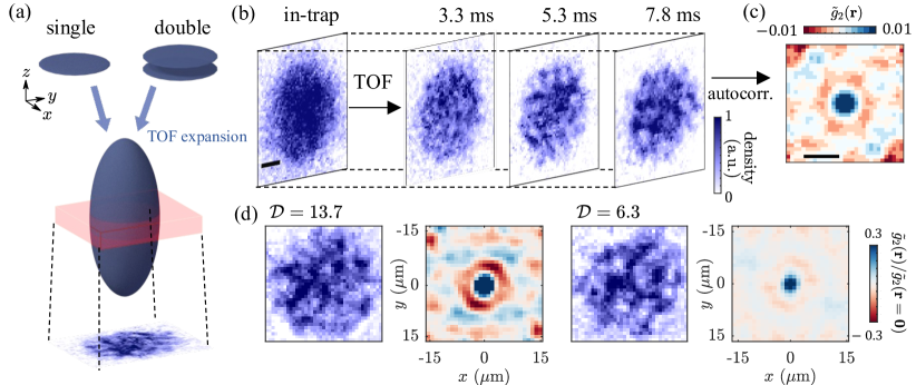
Figure 1: Noise interferometry of 2D Bose gases. (a) Sketch of the noise detection. We trap single- or double-layer ultracold 2D Bose gases with tight vertical confinement, and release them for a time-of-flight (TOF) expansion of duration $t$. The tight vertical confinement results in a fast vertical expansion of the cloud without significant expansion in the radial direction. We record a slice of the density distribution using absorption imaging with a selective optical repumping technique (red transparent sheet), which is necessary since the Rayleigh length of the high-resolution imaging apparatus is smaller than the vertical extent of the cloud after the expansion. (b) Single-shot images of the density distribution of trapped single-layer clouds with no expansion (in-situ) and at $t=3.3$, 5.3 and 7.8 $\text{\,}\mathrm{ms}$. (c) The noise correlation function $\tilde{g}_{2}(\bm{r})$, obtained by calculating the density-density correlations and averaging over experimental repeats; see text. A characteristic ring structure emerges at distance $|\bm{r}|\sim 7$\text{\,}\mathrm{\SIUnitSymbolMicro m}$$ due to density modulations that are present in the expanded cloud at $t=$7.8\text{\,}\mathrm{ms}$$. The black bars in panels (b) and (c) denote $10\text{\,}\mathrm{\SIUnitSymbolMicro m}$. (d) Typical single-shot density distribution and $\tilde{g}_{2}(\bm{r})$ shown after $t=$5.3\text{\,}\mathrm{ms}$$ for decoupled bilayer systems with phase-space densities of $\mathcal{D}=13.7$ and $6.3$.

We prepare 2D degenerate Bose gases of $\mathrm{{}^{87}Rb}$ atoms in a cylindrically-symmetric trap having strong confinement along the $z$ direction. In this work, we create single-well or double-well vertical confinement using either a single-RF or multiple-RF dressing technique, described in [23, 24, 25, 26, 22]. The single well and each potential minimum of double well have vertical trap frequencies of $\omega_{z}/2\pi=$1.2\text{\,}\mathrm{k}\mathrm{H}\mathrm{z}$$. This results in the dimensionless 2D interaction strength $\tilde{g}=\sqrt{8\pi}a_{s}/\ell_{0}=0.08$, where $a_{s}$ is the 3D scattering length, $\hbar$ is the reduced Planck constant and $\ell_{0}=\sqrt{\hbar/(m\omega_{z})}$ is the harmonic oscillator length along $z$ for an atom of mass $m$. We impose additional optical trapping in the horizontal plane using a ring-shaped strong off-resonant laser beam to realize near-homogeneous 2D systems [27]. We load atoms into the trap at a temperature $T=$50\text{\,}\mathrm{nK}$$, set by forced evaporation. For double-well potentials we work with equal population $N$ in each layer, achieved by maximizing the matter-wave interference contrast [26, 22]. We use a large inter-well separation of $7\text{\,}\mathrm{\SIUnitSymbolMicro m}$ to create a decoupled bilayer system. We vary $N$ to cover a broad range of the phase-space density $\mathcal{D}=nh^{2}/(2\pi mk_{B}T)$ between $5$ and $24$, where $n$ is the average 2D density and $k_{B}$ is the Boltzmann constant. For all parameters employed, the quasi-2D conditions $\hbar\omega_{z}>k_{B}T$ and $\hbar\omega_{z}>\mu$ are satisfied, where $\mu$ is the chemical potential.

The detection scheme is illustrated in Fig. 1(a). The trap is abruptly turned off to release the 2D gas for a time-of-flight (TOF) expansion of duration $t$ between 3.3 and 7.8 ms [28, 22] starting with either one or two clouds. Once released, the clouds expand ballistically along the $z$ direction while showing negligible expansion in the radial direction. We image a slice of the expanded clouds with thickness $L_{z}=$10\text{\,}\mathrm{\SIUnitSymbolMicro m}$$ along the z direction which is much smaller than the extent of the expanded cloud in this direction, as illustrated in Fig. 1(a). This ensures that the imaged sample is thin compared to the depth of field of the high-resolution imaging system [27]; further, we carefully focus the imaging system using the density-noise patterns as described in the Suppl. Mat. [27]. This minimizes the systematic effect of imperfect imaging on the density pattern measurements [10, 29]. Examples of the density distribution after several values of the TOF duration $t$, including the in-situ density distribution at $t=0$, are shown in Fig. 1(b). The system is deep in the superfluid regime with peak PSD of $\mathcal{D}=24$ [22, 27]. Compared to the in-situ density distribution, the expanded cloud shows the formation of density modulations on a length scale growing with $t$. This is due to self-interference of the cloud with constructive interference occurring at distances that depend on $t$ [13, 10, 14]. As a result, initial phase fluctuations transform into density modulations that we analyze to characterize the BKT transition. We autocorrelate the normalized density distribution in each cloud and then average the density-density correlations over at least 20 repetitions of the experiment. Thus, we obtain the noise correlation function [27, 14]

$$g_{2}(\bm{r},t)=\frac{\langle\Psi^{\dagger}(\bm{r},t)\Psi^{\dagger}(\bm{0},t)\Psi(\bm{r},t)\Psi(\bm{0},t)\rangle}{n(\bm{r},t)n(\bm{0},t)}.$$ (1)

In Fig. 1(c), we show $\tilde{g}_{2}(\bm{r})\equiv g_{2}(\bm{r})-1$ at $t=$7.8\text{\,}\mathrm{ms}$$, which features a characteristic minimum at distance $r\sim$7\text{\,}\mathrm{\SIUnitSymbolMicro m}$$ as predicted from the theoretical model [14]. We repeat these measurements for a decoupled bilayer system. Examples of single-shot density distribution and averaged noise correlation function $\tilde{g}_{2}(\bm{r},t)$, taken with $t=$5.3\text{\,}\mathrm{ms}$$ for the systems at $\mathcal{D}=13.7$ and $6.3$, are shown in Fig. 1(d). The existence of the characteristic minimum at high $\mathcal{D}$ is a feature of the superfluid phase, which is suppressed for the normal phase at lower $\mathcal{D}$ [14].

To infer the properties of the system we analyze how $g_{2}(\bm{r},t)$ depends on the expansion time and the in-situ phase fluctuations. Analysis of free expansion of a single-layer 2D quasicondensate with phase fluctuations yields $g_{2}(\bm{r},t)$ as a function of expansion time $t$ [13, 14, 27]

$$g_{2}(\bm{r},t)=\frac{1}{(2\pi)^{2}}\int d^{2}\bm{q}\int d^{2}\bm{R}\cos(\bm{q}\cdot\bm{r})\cos(\bm{q}\cdot\bm{R})$$

$$\times\frac{\mathcal{F}(\bm{q}_{t})^{2}\mathcal{F}(\bm{R})^{2}}{\mathcal{F}(\bm{R}-\bm{q}_{t})\mathcal{F}(\bm{R}+\bm{q}_{t})},$$ (2)

where $\bm{q}_{t}=\hbar\bm{q}t/m$ with $\bm{q}$ being the wave vector and the functions $\mathcal{F}$ are the first-order correlation functions i.e. $\mathcal{F}(\bm{r})\sim g_{1}(\bm{r})$. The analysis of $g_{2}(\bm{r},t)$ using algebraic and exponential forms of $g_{1}(\bm{r})$ predicts distinctive behaviors, which we utilize to probe the BKT transition [14, 27].

In Fig. 2(a), we show the measurements of $\tilde{g}_{2}(r,t)$ for a single-layer cloud deep in the superfluid regime, with $\mathcal{D}=24$, for several expansion times $t$. We shift the locations of the trapped cloud with a magnetic bias field along $z$ for each $t$, without changing any system parameters such as trap geometry, temperature and atom number, such that the expanded cloud is at the focus of the imaging apparatus after expansion time $t$. For the quantitative analysis, we determine the radially averaged $g_{2}(r,t)$ as a function of the radial coordinate $r$. Oscillatory behavior emerges for expanded clouds, which is absent for in-trap measurements. We fit the measurements at finite $t$ with the predictions of Eq. (Detecting Phase Coherence of 2D Bose Gases via Noise Correlations) for the superfluid phase to determine the superfluid exponent $\eta$ and the short-range cutoff $a$. The superfluid model describes our measurements well, with consistent values of $\eta\simeq 0.04$ and $a\simeq$3\text{\,}\mathrm{\SIUnitSymbolMicro m}$$ for all three expansion times as expected for the same in-situ system parameters, see Figs. 2 (b,c). To further corroborate the expansion scaling, we compare the locations $r_{1}$ of the first minimum of $\tilde{g}_{2}(r,t)$ with the mean-field prediction $r_{1}{}^{2}=3\pi\hbar t/m$ and the predictions of the superfluid model, see inset of Fig. 2 (a).

Figure 2: Expansion scaling behavior. (a) Radially averaged correlation function $\tilde{g}_{2}(r,t)$ is shown for trapped single-layer clouds with no expansion (in-situ) and after $t=3.3$, 5.3 and 7.8 $\text{\,}\mathrm{ms}$. Error bars are the standard error. Solid lines are the best fits based on Eq. (Detecting Phase Coherence of 2D Bose Gases via Noise Correlations) for the superfluid phase, from which we determine the superfluid exponent $\eta$ and the short-range cutoff $a$. Inset shows the squared locations $r_{1}^{2}$ of the first minimum of the correlation function (dots), together with the mean-field prediction $r_{1}{}^{2}\propto t$ (dashed line). The solid line shows the analytical prediction of the minimum position in the superfluid phase based on Eq. (Detecting Phase Coherence of 2D Bose Gases via Noise Correlations), including the effect of finite imaging resolution encoded in the short-range cutoff. (b, c) Extracted values of $\eta$ and $a$.

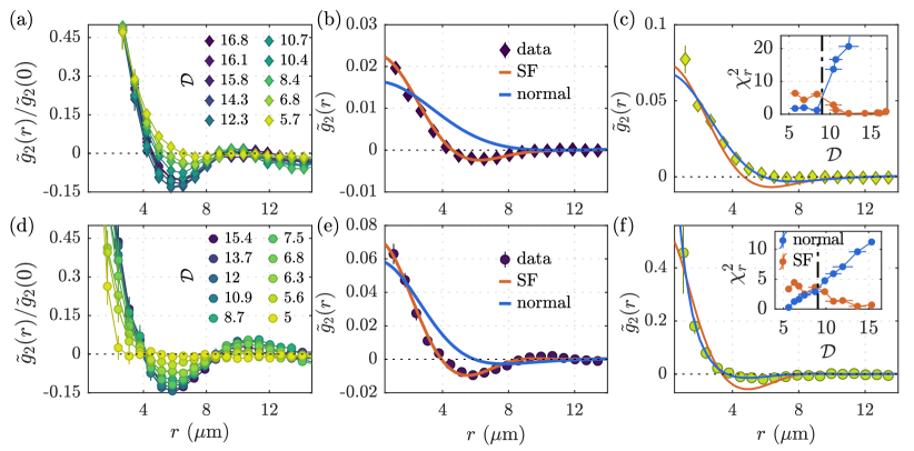
Figure 3: Noise correlations of single layer and bilayer 2D Bose gases across the BKT transition. (a) $\tilde{g}_{2}(r)$, scaled by the value at origin $\tilde{g}_{2}(0)$, is shown after $t=5.3$ ms for single-layer clouds having phase-space densities between $\mathcal{D}=5.7$ and $16.8$. Lines are guides to the eye and error bars are the standard error. (b) $\tilde{g}_{2}(r)$ at $\mathcal{D}=16.8$, plotted together with best fits of superfluid (SF, orange) and normal phase (blue) based on Eq. (Detecting Phase Coherence of 2D Bose Gases via Noise Correlations). (c) Measurement at $\mathcal{D}=5.7$ is well described by the prediction of the normal phase. Inset shows the reduced $\chi^{2}$ statistics of the superfluid and normal-phase fitting models at varying $\mathcal{D}$ (values for the normal phase at high $\mathcal{D}$ with $\chi_{r}^{2}>20$ are not shown). The crossover from superfluid to normal phase is identified by the point (vertical dashed line) beyond which $\tilde{g}_{2}(r)$ is better described by the normal-phase model at small $\mathcal{D}$. This yields the crossover at $\mathcal{D}_{c}=9.1(9)$. (d) Measurements after $t=5.3$ ms for bilayer clouds with phase-space densities between $\mathcal{D}=5$ and $15.4$. (e) $\tilde{g}_{2}(r)$ and their fitted curves at $\mathcal{D}=15.4$. (f) The measurement at $\mathcal{D}=5.6$ is better described by the normal-phase model, similarly to the single-layer case at small $\mathcal{D}$ in panel (c). Inset showing the $\chi_{r}^{2}$ errors of the fitting model, whose intersection gives the BKT crossover at $\mathcal{D}_{c}=9.0(6)$ (vertical dash-dotted line).

Having verified the expansion scaling behavior, we now turn our attention to the measurements across the BKT critical point, both with single and uncoupled bilayer 2D clouds. In Fig. 3(a), we show the measurements of $\tilde{g}_{2}(r)$ for single-layer clouds at varying $\mathcal{D}$. As $\mathcal{D}$ is lowered, the oscillatory feature of the noise correlations, characteristic of the superfluid phase, vanishes indicating a crossover to the normal phase. To verify this we fit the measurements with the predictions of Eq. (Detecting Phase Coherence of 2D Bose Gases via Noise Correlations) calculated for both the superfluid and normal phase. Examples of the fits are shown in Figs. 3 (b-c) for both large and small $\mathcal{D}$; for $\mathcal{D}=16.8$ the prediction for the superfluid phase gives a better fit, whereas for $\mathcal{D}=5.7$ it is the normal phase. We determine the BKT crossover point as being the value of $\mathcal{D}$ at which the exponential model overtakes the superfluid model, see inset of Fig. 3(c). This gives the crossover point at $\mathcal{D}_{c}=9.1(9)$, which is in close agreement with the theoretical prediction $\mathcal{D}_{c,th}=8.6$ [30].

In Fig. 3(d) we show the measurements of our bilayer systems at varying $\mathcal{D}$. Similar to the single-layer case, the noise correlations are oscillatory at large $\mathcal{D}$, however, there is a fast short-distance fall off of correlations in the normal regime at small $\mathcal{D}$. This is the characteristics of density-noise functions for bilayer systems, as we discuss in the following. For a bilayer 2D Bose gas characterized by the field operators $\Psi_{i}(\bm{r},t)$ for layers $i=1,2$, the density noise pattern measured along the $z$ axis is dominantly produced by the common-mode fluctuations with correlation function $\mathcal{F}_{\mathrm{com}}(\bm{r})^{2}\simeq\langle\Psi_{1}^{\dagger}(\bm{r})\Psi^{\dagger}_{2}(\bm{r})\Psi_{1}(\bm{0})\Psi_{2}(\bm{0})\rangle/n^{2}$, i.e. the noise correlation function of the expanded bilayer, which is defined by replacing the field operators in Eq. (1) by $\Psi(\bm{r},t)=(\Psi_{1}(\bm{r},t)+\Psi_{2}(\bm{r},t))/\sqrt{2}$. For a decoupled bilayer the noise correlation function is [27]

$$g_{2}(\bm{r},t)\approx\dfrac{1}{(2\pi)^{2}}\int d^{2}\bm{q}\int d^{2}\bm{R}\cos(\bm{q}\cdot\bm{r})\cos(\bm{q}\cdot\bm{R})$$

$$\times\dfrac{\mathcal{F}_{\mathrm{com}}(\bm{q}_{t})^{2}\mathcal{F}_{\mathrm{com}}(\bm{R})^{2}}{\mathcal{F}_{\mathrm{com}}(\bm{R}-\bm{q}_{t})\mathcal{F}_{\mathrm{com}}(\bm{R}+\bm{q}_{t})}\mathcal{F}_{\mathrm{rel}}(\bm{q}_{t})^{2},$$ (3)

where finite mixing of relative phase modes with correlation function $\mathcal{F}_{\mathrm{rel}}(\bm{r})^{2}\simeq\langle\Psi_{1}^{\dagger}(\bm{r})\Psi_{2}(\bm{r})\Psi_{2}^{\dagger}(\bm{0})\Psi_{1}(\bm{0})\rangle/n^{2}$ affects $g_{2}(\bm{r},t)$ in the normal regime, resulting in a fast decay of $|g_{2}|$ at short distances, see Fig. S1 in [27]. We calculate the predictions of Eq. (Detecting Phase Coherence of 2D Bose Gases via Noise Correlations) for the superfluid and normal regimes and use them to fit our bilayer noise correlations to determine the exponent $\eta$ and the BKT crossover, see Figs. 3 (d-f). The BKT crossover occurs at $\mathcal{D}_{c}=9.0(6)$, which is in agreement with the results of the single layer behavior and the theoretical prediction [30]. Combined with the relative-mode phase correlation measurements using matter-wave homodyning [31, 22], this method gives a complete characterization of phase fluctuations of bilayer systems. The relative and common modes have the same statistics in the absence of interlayer coupling, which we utilize to benchmark the results of the noise measurements [22, 27], as we discuss below.

In Fig. 4 we consolidate the results of single and bilayer 2D clouds. The measured value of $\eta$ scales linearly with the inverse phase-space density $\mathcal{D}^{-1}$ in the superfluid regime, which is in accordance with the Nelson-Kosterlitz relation $\eta\propto\mathcal{D}^{-1}$ [32, 22]. We find a deviation from this linear behavior when the system approaches the crossover regime at $\mathcal{D}^{-1}=$ 0.11(1), as predicted [22]: in the normal phase above the broad crossover regime $\eta$ shows a faster increase within the measurement uncertainty. The determination of $\eta$ is less accurate in the normal regime since the correlations are short ranged and better described by exponential scaling. We also show the values of $\eta$ obtained from the relative-phase correlation measurements [27, 22], which are in agreement with the results of the noise measurements.

In conclusion, we have demonstrated a novel experimental technique to probe phase fluctuations in 2D Bose gases through the correlation analysis of density noise patterns appearing after short time-of-flight (TOF) expansions. The location $r_{1}$ of first minimum of the measured noise correlation function $g_{2}(r,t)$ scales with the expansion time $t$ as $r_{1}^{2}\propto t$. This confirms the expansion scaling and demonstrates that the determined values of the superfluid exponent and the BKT critical point are independent of the expansion time. The noise interferometry of expanded bilayer systems and extraction of common-mode phase correlations in two-mode 2D Bose gases, was benchmarked by exploiting the fact that it has the same behavior as the relative-mode correlation function in the absence of interlayer coupling.

The spatial noise interferometry method for quantum gases presented in this Letter, used together with the direct matter-wave interferometric probe of relative phase mode [22], supports the development of a more comprehensive understanding of novel many-body phases of matter arising from coherent coupling of bilayer 2D quantum systems [18, 33, 34, 35, 36, 27] and out-of-equilibrium dynamics of coupled 2D quantum systems following a quench [20, 21, 18, 37], for which the measurement of two complementary relative and common modes is crucial.

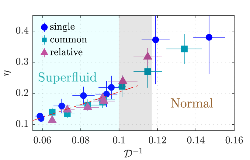
Figure 4: The BKT crossover in 2D Bose gases. The algebraic exponent $\eta$ is plotted as a function of the inverse phase-space density $\mathcal{D}^{-1}$. Results for a single layer (circles) and bilayer (squares) are compared against the measurements (triangles) of the relative-phase correlations [27]. Red dash-dotted line is the Nelson-Kosterlitz relation $\eta\propto\mathcal{D}^{-1}$, expected in the superfluid regime [32]. The crossover region (black shaded area) is at $\mathcal{D}^{-1}=$ 0.11(1), corresponding to a critical algebraic exponent $\eta_{c}\sim 0.2$ as expected for a finite-sized system [22]. Above the critical point, values of $\eta$ have increased uncertainty as the in-situ phase correlations become short ranged.

Supplemental Material

.1 Density-noise correlation function of expanded bilayer 2D Bose gases

In this section, we analyze the density noise correlation function of expanded bilayer systems to obtain the expression based on in-situ correlation properties, following the derivation for the single layer systems in Ref. [14]. The bilayer system consists of two layers $i=1,2$ initially separated in the $z$ direction with separation $d$, where $d=$7\text{\,}\mathrm{\SIUnitSymbolMicro m}$$ for the experiments reported in the main text, and we express the two layers using bosonic field operators $\Psi_{i}(\bm{r})$. We take the initial 3D wavefunction to be of the form

$$\hat{\bm{\Psi}}_{0}(\bm{r}_{2D},z;t)=[\hat{\bm{\Psi}}_{1}(\bm{r})\delta(d-z)+\hat{\bm{\Psi}}_{2}(\bm{r})\delta(d+z)]/\sqrt{2},$$ (S1)

and analyze its expansion dynamics. Free expansion of the bosonic field operator is given by

$$\hat{\bm{\Psi}}(\bm{r},t)=\int d^{3}\bm{r}^{\prime}G_{3}(\bm{r}-\bm{r}^{\prime},t)\hat{\bm{\Psi}}(\bm{r}^{\prime},0),$$ (S2)

where the 3D Green’s function is

$$G_{3}(\bm{r}-\bm{r}^{\prime},t)=G_{1}(x-x^{\prime},t)G_{1}(y-y^{\prime},t)G_{1}(z-z^{\prime},t),$$ (S3)

and

$$G_{1}(r,t)=\sqrt{\frac{m}{2\pi i\hbar t}}e^{\frac{im}{2\hbar t}r^{2}}.$$ (S4)

Combining the prefactors into $A=\frac{m}{2\pi\hbar t}$, the density distribution after the TOF expansion is

$$\hat{n}(\bm{r},t)=A^{3}\int d^{3}\bm{v}\int d^{3}\bm{w}\ e^{\frac{-im}{2\hbar t}(\bm{r}-\bm{v})^{2}}\hat{\bm{\Psi}}^{{\dagger}}(\bm{v},0)e^{\frac{im}{2\hbar t}(\bm{r}-\bm{w})^{2}}\hat{\bm{\Psi}}(\bm{w},0).$$ (S5)

Following the procedure in Ref. [14], denoting the spatial coordinates in the $xy$-plane by the subscript $\parallel$ and coordinates perpendicular to it (i.e. in the $z$ direction) by the subscript $\bot$, the density-density correlation function is

$$g_{2}(\bm{r}_{1},\bm{r}_{2},t)= \frac{A^{4}}{4n_{0}^{2}}\int d^{2}\bm{r}\int d^{2}\bm{r}^{\prime}\int ds_{\bot}\int dS_{\bot}\int du_{\bot}\int dU_{\bot}$$ (S6)

$$\times e^{\frac{-im}{4\hbar t}\left[\bm{r}^{2}-\bm{r}^{\prime 2}-2\bm{r}_{\parallel 12}\cdot(\bm{r}-\bm{r}^{\prime})\right]}\times e^{\frac{-im}{\hbar t}\left[(S_{\bot}-\frac{r_{\bot 12}}{2})s_{\bot}+(U_{\bot}+\frac{r_{\bot 12}}{2})u_{\bot}-R_{\bot 12}(s_{\bot}+u_{\bot})\right]}$$

$$\times\biggl{<}\hat{\bm{\Psi}}_{0}^{{\dagger}}(\frac{\bm{r}}{2},S_{\bot}+\frac{s_{\bot}}{2})\hat{\bm{\Psi}}_{0}^{{\dagger}}(-\frac{\bm{r}}{2},U_{\bot}+\frac{u_{\bot}}{2})\hat{\bm{\Psi}}_{0}(\frac{\bm{r}^{\prime}}{2},S_{\bot}-\frac{s_{\bot}}{2})\hat{\bm{\Psi}}_{0}(-\frac{\bm{r}^{\prime}}{2},U_{\bot}-\frac{u_{\bot}}{2})\biggr{>},$$

where we use center of mass coordinates, $\bm{r}_{12}=\bm{r}_{1}-\bm{r}_{2}$ and $\bm{R}_{12}=(\bm{r}_{1}+\bm{r}_{2})/2$. With integration along the $z$ direction with sufficient integration width, equivalent to the imaging procedure in the experiment reported in the main text [38], we obtain in terms of 2D coordinates,

$$\tilde{g}_{2}(\bm{r}_{1,2D},\bm{r}_{2,2D})=\int dr_{1z}\int dr_{2z}g_{2}(\bm{r}_{1,3D},\bm{r}_{2,3D}),$$ (S7)

where the integration over $r_{1z}$, $r_{2z}$ (or $R_{\bot 12}$ and $r_{\bot 12}$), gives delta functions for $u_{\bot}$ and $s_{\bot}$. The delta functions result in $s_{\bot}=-u_{\bot}$ and $s_{\bot}=u_{\bot}=0$ and thus modify the prefactor, such that

$$\tilde{g}_{2}(\bm{r}_{1,2D},\bm{r}_{2,2D})=\frac{A^{2}}{4n_{0}^{2}}\int d^{2}\bm{r} \int d^{2}\bm{r}^{\prime}\int dS_{\bot}\int dU_{\bot}e^{\frac{-im}{4\hbar t}\left[\bm{r}^{2}-\bm{r}^{\prime 2}-2\bm{r}_{\parallel 12}\cdot(\bm{r}-\bm{r}^{\prime})\right]}$$ (S8)

$$\times\biggl{<}\hat{\bm{\Psi}}_{0}^{{\dagger}}(\frac{\bm{r}}{2},S_{\bot})\hat{\bm{\Psi}}_{0}^{{\dagger}}(-\frac{\bm{r}}{2},U_{\bot})\hat{\bm{\Psi}}_{0}(\frac{\bm{r}^{\prime}}{2},S_{\bot})\hat{\bm{\Psi}}_{0}(-\frac{\bm{r}^{\prime}}{2},U_{\bot})\biggr{>}.$$

We now reintroduce the original $z$ spatial variables, $S_{\bot}=(z_{1}+z_{2})/2$, $s_{\bot}=z_{1}-z_{2}$ and $U_{\bot}=(z_{3}+z_{4})/2$, $u_{\bot}=z_{3}-z_{4}$. With the delta functions for $s_{\bot}$ and $u_{\bot}$ described above we have $S_{\bot}=z_{1}$, $U_{\bot}=z_{3}$, so that

$$\tilde{g}_{2}(\bm{r}_{1,2D},\bm{r}_{2,2D})=\frac{A^{2}}{4n_{0}^{2}}\int d^{2}\bm{r} \int d^{2}\bm{r}^{\prime}\int dz_{1}\int dz_{3}e^{\frac{-im}{4\hbar t}\left[\bm{r}^{2}-\bm{r}^{\prime 2}-2\bm{r}_{\parallel 12}\cdot(\bm{r}-\bm{r}^{\prime})\right]}$$ (S9)

$$\times\biggl{<}\hat{\bm{\Psi}}_{0}^{{\dagger}}(\frac{\bm{r}}{2},z_{1})\hat{\bm{\Psi}}_{0}^{{\dagger}}(-\frac{\bm{r}}{2},z_{3})\hat{\bm{\Psi}}_{0}(\frac{\bm{r}^{\prime}}{2},z_{1})\hat{\bm{\Psi}}_{0}(-\frac{\bm{r}^{\prime}}{2},z_{3})\biggr{>}.$$

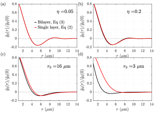
Figure S1: Theoretical model of bilayer density-noise correlation functions with (red) and without (black) considering the mixing of relative phase effect, for (a,b) superfluid regime, and (c,d) normal regime. The theoretical curves are obtained by the numerical integration of Eqs. (Detecting Phase Coherence of 2D Bose Gases via Noise Correlations) and (S15) in a similar manner to Ref. [14], where for both common-mode and relative-mode correlation function $\mathcal{F}_{\mathrm{com}}$ and $\mathcal{F}_{\mathrm{rel}}$ are taken to be the first-order correlation function of a single layer system, as applicable for a decoupled bilayer.

To simplify notation we introduce

$$\rho_{ijkl}(\bm{r},\bm{r}^{\prime})=\biggl{<}\hat{\bm{\Psi}}_{i}^{{\dagger}}(\frac{\bm{r}}{2})\hat{\bm{\Psi}}_{j}^{{\dagger}}(-\frac{\bm{r}}{2})\hat{\bm{\Psi}}_{k}(\frac{\bm{r}^{\prime}}{2})\hat{\bm{\Psi}}_{l}(-\frac{\bm{r}^{\prime}}{2})\biggr{>}.$$ (S10)

Substituting Eq. S1 into Eq. S9 and evaluating the $z_{1}$ and $z_{2}$ integrals,

$$\tilde{g}_{2}(\bm{r}_{1,2D},\bm{r}_{2,2D})=\frac{A^{2}}{4n_{0}^{2}} \int d^{2}\bm{r}\int d^{2}\bm{r}^{\prime}e^{\frac{-im}{4\hbar t}\left[\bm{r}^{2}-\bm{r}^{\prime 2}-2\bm{r}_{\parallel 12}\cdot(\bm{r}-\bm{r}^{\prime})\right]}$$ (S11)

$$\times\frac{1}{4}\biggl{[}\rho_{1111}(\bm{r},\bm{r}^{\prime})+\rho_{2121}(\bm{r},\bm{r}^{\prime})+\rho_{1212}(\bm{r},\bm{r}^{\prime})+\rho_{2222}(\bm{r},\bm{r}^{\prime})\biggr{]}.$$

Using the density-phase representation of the Bose field in the trap, $\Psi(\bm{r})\simeq\sqrt{n}\exp(i\phi(\bm{r}))$, applicable for our case of quasicondensates [39], Eq. (S10) can be represented by the phase fluctuation as $\rho_{ijkl}(\bm{r},\bm{r}^{\prime})\sim n_{0}^{2}\left<e^{i[\theta_{i}(\bm{r}/2)+\theta_{j}(-\bm{r}/2)-\theta_{k}(\bm{r}^{\prime}/2)-\theta_{l}(-\bm{r}^{\prime}/2)]}\right>$ where $\theta(\bm{r})=(\phi_{1}(\bm{r})-\phi_{2}(\bm{r}))/2$, $\varphi(\bm{r})=(\phi_{1}(\bm{r})+\phi_{2}(\bm{r}))/2$ are the antisymmetric and symmetric phase modes. Writing the complex exponentials using cosines, the density-density correlation function of expanded cloud is

$$\tilde{g}_{2}(\bm{r}_{1,2D},\bm{r}_{2,2D})=\frac{A^{2}}{4n_{0}^{2}} \int d^{2}\bm{r}\int d^{2}\bm{r}^{\prime}e^{\frac{-im}{4\hbar t}\left[\bm{r}^{2}-\bm{r}^{\prime 2}-2\bm{r}_{\parallel 12}\cdot(\bm{r}-\bm{r}^{\prime})\right]}$$ (S12)

$$\times\rho_{\varphi}(\bm{r},\bm{r}^{\prime})\biggl{<}\cos(\Delta\theta(\bm{r},\bm{r}^{\prime}))\cos(\Delta\theta(-\bm{r},-\bm{r}^{\prime}))\biggr{>},$$

where $\rho_{\varphi}(\bm{r},\bm{r}^{\prime})=n_{0}^{2}\left<e^{i[\varphi(\bm{r}/2)+\varphi(-\bm{r}/2)-\varphi(\bm{r}^{\prime}/2)-\varphi(-\bm{r}^{\prime}/2)]}\right>$ expresses the common-mode phase correlation which dominantly contributes to the measured density noise correlation; the final term containing $\Delta\theta(\bm{r},\bm{r}^{\prime})=\theta(\bm{r}/2)-\theta(\bm{r}^{\prime}/2)$ encapsulates the effect of finite mixing of relative phase on $\tilde{g}_{2}$. Introducing the shorthand notation $\Delta\theta(\pm)=\Delta\theta(\pm\bm{r},\pm\bm{r}^{\prime})$, this term can be expressed as exponentials

$$\biggl{<}\cos(\Delta\theta(+))\cos(\Delta\theta(-))\biggr{>}=\frac{1}{4}\biggl{<}e^{i[\Delta\theta(+)+\Delta\theta(-)]}+e^{i[\Delta\theta(+)-\Delta\theta(-)]}+e^{i[-\Delta\theta(+)+\Delta\theta(-)]}+e^{i[-\Delta\theta(+)-\Delta\theta(-)]}\biggr{>},$$ (S13)

assuming Gaussian phase fluctuations $\left<e^{i[\theta(r)+\theta(r^{\prime})]}\right>=e^{-\frac{1}{2}\left<[\theta(r)+\theta(r^{\prime})]^{2}\right>}$. Defining the relative-phase correlation function $\mathcal{F}_{\mathrm{rel}}(\bm{r}-\bm{r}^{\prime})\equiv\left<e^{i[\theta(\bm{r})-\theta(\bm{r}^{\prime})]}\right>\simeq\langle\hat{\Psi}_{1}^{\dagger}(\bm{r},0)\hat{\Psi}_{2}(\bm{r},0)\hat{\Psi}_{2}^{\dagger}(\bm{0},0)\hat{\Psi}_{1}(\bm{0},0)\rangle/n_{0}^{2}$ and expanding the exponents for each term in Eq. S13,

$$\biggl{<}\cos(\Delta\theta(+))\cos(\Delta\theta(-))\biggr{>}\approx\mathcal{F}_{\mathrm{rel}}([\bm{r}-\bm{r}^{\prime}]/2)^{2},$$ (S14)

to linear order in $\left<\Delta\theta(-)\Delta\theta(+)\right>$. Thus the density correlation function is

$$\tilde{g}_{2}(\bm{r}_{1,2D},\bm{r}_{2,2D})\approx\frac{A^{2}}{4n_{0}^{2}}\int d^{2}\bm{r}\int d^{2}\bm{r}^{\prime}e^{\frac{-im}{4\hbar t}\left[\bm{r}^{2}-\bm{r}^{\prime 2}-2\bm{r}_{\parallel 12}\cdot(\bm{r}-\bm{r}^{\prime})\right]}\rho_{\varphi}(\bm{r},\bm{r}^{\prime})\mathcal{F}_{\mathrm{rel}}([\bm{r}-\bm{r}^{\prime}]/2)^{2}.$$ (S15)

Following the procedure for the case of a single layer [14] we perform a change of variables, $\bm{q}=(m/2\hbar t)(\bm{r}-\bm{r}^{\prime})$, $\bm{R}=(\bm{r}+\bm{r}^{\prime})/2$, effectively resulting in a Fourier transform. Rewriting the result using $\mathcal{F}_{\mathrm{com}}(\bm{r})$ and $\bm{q}_{t}$ defined as in the main text, gives

$$\tilde{g}_{2}(\bm{r},t)\approx\frac{1}{(2\pi)^{2}}\int d^{2}\bm{q}\int d^{2}\bm{R}\cos(\bm{q}\cdot\bm{r})\cos(\bm{q}\cdot\bm{R})\frac{\mathcal{F}_{\mathrm{com}}(\bm{q}_{t})^{2}\mathcal{F}_{\mathrm{com}}(\bm{R})^{2}}{\mathcal{F}_{\mathrm{com}}(\bm{R}-\bm{q}_{t})\mathcal{F}_{\mathrm{com}}(\bm{R}+\bm{q}_{t})}\mathcal{F}_{\mathrm{rel}}(\bm{q}_{t})^{2}.$$ (S16)

In Fig. S1, we compare Eq. (Detecting Phase Coherence of 2D Bose Gases via Noise Correlations) and Eq. (Detecting Phase Coherence of 2D Bose Gases via Noise Correlations), the density-noise correlation functions for the single-layer and bilayer systems. The difference between the two models are evident deep in the normal regime with correlation length $r_{0}$ much smaller than the system size used in the experiment, $\sim$30\text{\,}\mathrm{\SIUnitSymbolMicro m}$$. We use the numerically integrated functions of Eq. Detecting Phase Coherence of 2D Bose Gases via Noise Correlations (Eq. Detecting Phase Coherence of 2D Bose Gases via Noise Correlations) for the fitting of experimental data taken with single-layer (bilayer) systems [14]. The expression Eq. (S16) holds in the presence of inter-layer tunnel-coupling as the relative and common modes fluctuate independently, both having Gaussian fluctuations for the experimentally relevant range of inter-layer coupling strengths [40].

.2 Experimental procedure

.2.1 Preparation of 2D Bose gases

We form the 2D potential for the laser-cooled $\mathrm{{}^{87}Rb}$ atoms using a combination of a static and radiofrequency (RF) magnetic fields [41]. The static field is a quadrupole magnetic field with cylindrical symmetry about a vertical axis, and an additional single-frequency RF magnetic field is used for creating a single 2D Bose gas. The RF frequency is 7.2 MHz with quadrupole field gradient of 150 G/cm along $z$, resulting in the trap parameters described in the main text. In contrast, three RF fields are applied to give a mutiple-RF (MRF) double-well trap, at 7.08, 7.2 and 7.32 MHz, for the experiments to obtain data for Figs. 3 and 4. Control over the amplitudes of RF components allows us to shape the double-well potential, as described in Refs. [41, 42, 25, 26], such that it provides tight confinement in the vertical direction to produce a 2D potential. We adiabatically load atoms into the MRF-dressed potential and let the system equilibrate for 500 ms, such that two quasicondensates are in equilibrium and individually fluctuating [22]. We ensure the populations in the two wells are equal by maximizing the observed matter-wave interference contrast as described in Ref. [26]. For the experiments for Figs. 3 and 4, the additional box optical potential is created by far-detuned $532\text{\,}\mathrm{nm}$ laser shaped with a spatial light modulator (digital micromirror device, DMD) realizing a ring-shaped repulsive trap, on top of the weak harmonic potential of the MRF-dressed potential having $\omega_{r}/2\pi=$8\text{\,}\mathrm{Hz}$$ (see Fig. S2). While the resulting density is not completely uniform, the homogeneity is significantly better than for the harmonic potential thanks to increased density near the center of the trap. We thus use the central region of the near-homogeneous system with radius of up to $15\text{\,}\mathrm{\SIUnitSymbolMicro m}$ for the data analysis. The optical potential is slowly ramped up for a second after loading atoms into the RF-dressed potentials, such that the introduction of this additional potential does not cause excitations in the system.

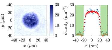
Figure S2: Near-homogeneous density distribution realized with ring-shaped repulsive optical trap. (left) Single-shot image of in-situ density distribution, taken along the $z$ direction. We apply repulsive optical dipole trap at 532 nm with ring-shaped geometry, generated by a DMD, onto trapped 2D Bose gases with weak harmonic confinement of $\omega_{r}/2\pi=$8\text{\,}\mathrm{Hz}$$. (right) 1D plot of data in left panel, along $y=0$ axis (blue) as well as radially-averaged density distribution (red). Green shaded region is where repulsive optical potential is applied.

.2.2 Alignment of the imaging system

Misalignment of the imaging system results in unintended artificial patterns in the obtained absorption images, affecting the density noise analysis [10, 29]. Therefore, in addition to the selective imaging technique (see Fig. 1), we utilized the density noise correlation patterns as a focusing target with small-scale structure to perform precise alignment of the imaging system. We have obtained the density-noise correlation functions at $t=$5.3\text{\,}\mathrm{m}\mathrm{s}$$, as described in the text, with varying static magnetic bias field to precisely shift the location of the trapped cloud, and hence the cloud after the TOF expansion. We move the location of the sheet of repumping light accordingly, to move the imaged sample without moving the imaging apparatus including the objective lens. In Fig. S3, we show the density-noise correlation functions at varying relative position of the cloud after the TOF (with colors corresponding to the data points in the inset). A clear change in the amplitude of the anticorrelation is observable, which is shown in inset as the change of minimum values of the correlation function. The negative peak is larger for sharper images, which indicates better focussing. We thus record the position of the atom after the TOF that minimizes the minimum value of the $\tilde{g}_{2}$ function, as the focal position of the imaging apparatus.

.2.3 Image analysis

The analysis of the density noise patterns proceeds as follows. From at least 20 experimental images for each experimental parameter, we first normalize the images by the average density distribution for each dataset. We then obtain autocorrelation of images within a region of interest (ROI) which captures the central part of the cloud. This results in a collection of correlation functions on a 2D grid, scaled by the squared mean density $n_{0}^{2}=\langle\hat{n}(\bm{r},t)\rangle^{2}=\langle\hat{\Psi}(\bm{r},t)^{\dagger}\hat{\Psi}(\bm{r},t)\rangle^{2}$, where $\hat{\Psi}(\bm{r},t)$ is the bosonic field operator after the expansion, which corresponds to [14, 27]

$$\frac{\langle\hat{n}(\bm{r},t)\hat{n}(\bm{0},t)\rangle}{n_{0}^{2}}=g_{2}(\bm{r},t)+\frac{\delta(\bm{r})}{n_{0}},$$ (S17)

where the second term is the shot-noise term with zero mean, such that

$$g_{2}(\bm{r},t)=\frac{\langle\hat{\Psi}^{\dagger}(\bm{r},t)\hat{\Psi}(\bm{r},t)\hat{\Psi}^{\dagger}(\bm{0},t)\hat{\Psi}(\bm{0},t)\rangle}{\langle\hat{n}(\bm{r},t)\rangle\langle\hat{n}(\bm{0},t)\rangle},$$ (S18)

is identified by averaging over experimental repetitions.

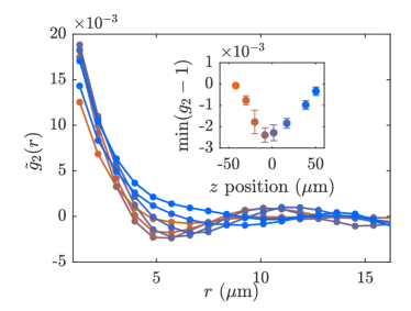
Figure S3: Focusing of the imaging apparatus by observation of the density-noise correlation functions. Correlation functions $\tilde{g}_{2}$, taken at $t=$5.3\text{\,}\mathrm{ms}$$ at $\mathcal{D}=24$, are plotted for varying values of static magnetic bias field along $z$ direction, which shifts the position of the atoms from $-50\text{\,}\mathrm{\SIUnitSymbolMicro m}$ to $50\text{\,}\mathrm{\SIUnitSymbolMicro m}$. We identify the optimal imaging configuration where the density pattern is most clearly resolved and amplitude of the anticorrelation peak of the $g_{2}$ is maximized (inset).

.3 Direct matter-wave interferometry readout of relative phase correlation function

To observe the matter-wave interference, the trap is abruptly turned off, releasing the pair of 2D gases for a time-of-flight (TOF) expansion of duration $t=$16.2\text{\,}\mathrm{m}\mathrm{s}$$. Once released, a matter-wave interference pattern along $z$ appears. We image a thin slice of the density distribution with thickness $L_{y}=$5\text{\,}\mathrm{\SIUnitSymbolMicro m}$$, as described in detail in Ref. [22].

We analyse the local phase of the matter-wave interference patterns following the procedure outlined in Refs. [26, 22], in which we perform a 1D fit of column density $\rho_{x}(z)$ at each location $x$ with

$$\rho_{x}(z)=\rho_{0}\exp\left(-z^{2}/2\sigma^{2}\right)\left[1+c_{0}\cos(kz+\theta(x))\right],$$ (S19)

where $\rho_{0},\sigma,c_{0},k,\theta(x)$ are fit parameters. The extracted phase $\theta(x)$ encodes a specific realisation of the fluctuations of the in situ local relative phase between the pair of 2D gases [22]. For each experimental run, we calculate the two-point phase correlation function $e^{i[\theta(x)-\theta(x^{\prime})]}$ at locations $x$ and $x^{\prime}$. We then determine the averaged correlation function

$$C^{(\mathrm{rel})}_{\mathrm{exp}}(x,x^{\prime})=\frac{1}{N_{r}}\sum_{j}e^{i[\theta(x)-\theta(x^{\prime})]},$$ (S20)

where the index $j$ runs over $N_{r}$ individual experimental realisations with $N_{r}>50$. We analyse the real part of the correlation function $C^{(\mathrm{rel})}(x,x^{\prime})=\text{Re}\left[C^{(\mathrm{rel})}_{\mathrm{exp}}(x,x^{\prime})\right]$, which is equal to $1$ for perfectly correlated pairs of points and $0$ for uncorrelated pairs of points. $C^{(\mathrm{rel})}_{\mathrm{exp}}(x,x^{\prime})$, is related to the relative phase correlation function

$$C^{(\mathrm{rel})}(\bm{r},\bm{r}^{\prime}):=\frac{\langle\Psi_{1}^{\dagger}(\bm{r})\Psi_{2}(\bm{r})\Psi_{2}^{\dagger}(\bm{r}^{\prime})\Psi_{1}(\bm{r}^{\prime})\rangle}{\langle|\Psi_{1}(\bm{r})|^{2}\rangle\langle|\Psi_{2}(\bm{r}^{\prime})|^{2}\rangle},$$ (S21)

For independently fluctuating layers, this is

$$C^{(\mathrm{rel})}(\bm{r},\bm{r}^{\prime})\simeq\frac{\langle\Psi^{\dagger}(\bm{r})\Psi(\bm{r^{\prime}})\rangle^{2}}{\langle|\Psi(\bm{r})|^{2}\rangle\langle|\Psi(\bm{r^{\prime}})|^{2}\rangle}=\frac{g_{1}({\bm{r},\bm{r}^{\prime}})^{2}}{n_{0}^{2}},$$ (S22)

where $n_{0}$ is the 2D density [22]. To quantify the decay of correlations, we calculate $C(\overline{x})$ by averaging $C^{(\text{rel})}(x,x^{\prime})$ over points with the same spatial separation $\overline{x}=x-x^{\prime}$ and perform fits with power-law models, obtaining the scaling of power-law exponent $\eta$ as shown in Fig. 4.