Highway Value Iteration Networks

Abstract

Value iteration networks (VINs) enable end-to-end learning for planning tasks by employing a differentiable “planning module” that approximates the value iteration algorithm. However, long-term planning remains a challenge because training very deep VINs is difficult. To address this problem, we embed highway value iteration—a recent algorithm designed to facilitate long-term credit assignment—into the structure of VINs. This improvement augments the “planning module” of the VIN with three additional components: 1) an “aggregate gate,” which constructs skip connections to improve information flow across many layers; 2) an “exploration module,” crafted to increase the diversity of information and gradient flow in spatial dimensions; 3) a “filter gate” designed to ensure safe exploration. The resulting novel highway VIN can be trained effectively with hundreds of layers using standard backpropagation. In long-term planning tasks requiring hundreds of planning steps, deep highway VINs outperform both traditional VINs and several advanced, very deep NNs.

1 Introduction

Planning is a search for action sequences that are predicted to achieve specific goals. The value iteration network (VIN) (Tamar et al., 2016) is a neural network (NN) architecture that enables end-to-end training for planning tasks using an embedded “planning module,” a differentiable approximation of the value-iteration algorithm (Bellman, 1966). VINs have exhibited remarkable proficiency in various tasks, including path planning (Pflueger et al., 2019; Jin et al., 2021), autonomous navigation (Wöhlke et al., 2021), and complex decision-making in dynamic environments (Li et al., 2021b).

However, VIN encounters significant challenges in long-term planning. For example, in path planning tasks where the shortest path length exceeds 120, the success rate of VINs in reaching the goal drastically decreases below 10% (Fig. 1). A promising approach to improve the long-term planning capabilities of VIN is increasing the depth of its embedded “planning module.” A deeper planning module can integrate more planning steps in VINs, potentially improving their ability to perform long-term planning.

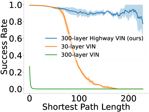
Figure 1: Success rates of reaching the goal in a $25\times 25$ maze problem. The success rate of a 30-layer VIN considerably decreases as the shortest path length increases, and training a 300-layer VIN is difficult and exhibits poor performance.

Nonetheless, increasing the depth of an NN can introduce complications, such as vanishing or exploding gradients, which is a fundamental problem in deep learning (Hochreiter, 1991). Although very deep NNs can be effectively trained in classification tasks using different methods (Srivastava et al., 2015b, a; He et al., 2016; Huang et al., 2017), these methods have not been equally successful in planning tasks (Table 1 in Section 5). This disparity may arise from the unique architecture of the VIN, particularly its planning module, which incorporates a specific inductive bias from reinforcement learning (RL). This inductive bias is grounded in the value iteration algorithm, known for its theoretical soundness (Bellman, 1966; Sutton & Barto, 2018). Herein, additional RL-relevant prior knowledge is integrated into the VIN architecture to address these challenges.

This study aims to integrate well-established techniques from both the fields of NNs and RL to create an effective and theoretically sound method. Central to the foundation of this proposed approach is highway value iteration (Wang et al., 2024). This method was designed to facilitate efficient long-term credit assignment in the context of RL. We also leverage the architectural innovations of highway networks (Srivastava et al., 2015b, a) and their variants residual networks (He et al., 2016) and DenseNets (Huang et al., 2017), particularly their use of skip connections, which are advantageous for training exceptionally deep NNs.

Building on this foundation, the VIN is enhanced by embedding the highway value iteration algorithm into its core “planning module.” This integration introduces three key innovations: (1) an “aggregate gate” for creating skip connections and improving information flow between layers; (2) an “exploration module” that injects controlled stochasticity during training, thereby diversifying information and gradient flow across spatial dimensions; (3) and a ”filter gate” designed to “filter out” useless exploration paths, ensuring safe and efficient exploration. These improvements result in the highway value iteration network (highway VIN), a new VIN variant specifically tailored for long-term planning. Remarkably, highway VINs can be efficiently trained with hundreds of layers using standard backpropagation techniques. This study highlights the connections between highway RL and highway networks and their combined potential to advance the capabilities of deep learning models in complex planning tasks. Notably, in scenarios requiring extensive planning, highway VINs outperform traditional VINs and several advanced deep NN models. This showcases their superior capability in handling complex, long-term planning challenges. The source code of highway VIN is available at https://github.com/wangyuhuix/HighwayVIN.

2 Related Work

Variants of Value Iteration Networks.

VINs (Tamar et al., 2016) are important architectures that integrate planning capabilities directly into NNs. VINs have a notable advantage over classical RL methods, as they learn policies that generalize better on novel tasks. However, VINs are challenged by issues such as training instability, hyperparameter sensitivity, and overestimation bias. These issues can be addressed using gated path-planning networks (GPPN) (Lee et al., 2018), a recurrent version of the VIN, which replaces convolutional networks with gated recurrent networks, resulting in more stable and effective learning. For higher-dimensional planning tasks, AVINs (Schleich et al., 2019) extend VINs with multi-level abstraction modules. These modules can capture various types of useful information during learning. Another significant challenge arises in generalizing VINs to target domains with limited data. Transfer VINs (Shen et al., 2020) tackle this issue by proposing a transfer learning approach, effectively adapting VINs to different, unseen target domains. Unfortunately, existing methods are considerably limited to extend to real-world and large-scale planning problems as shallow NNs lack long-term planning ability.

Neural Networks with Deep Architectures.

Deep learning involves assigning credits to NN components that affect the performance of the NN across multiple layers, or in the case of sequential data, over several time steps. In 1965, Ivakhnenko & Lapa (1965) introduced the first learning algorithms for deep feedforward NNs (FNNs) with any number of hidden layers. However, training FNNs with more than six layers by gradient descent remained a challenge until the early 2010s (Ciresan et al., 2010). Similarly, in the 1980s, recurrent neural networks (RNNs) were limited to problems spanning fewer than ten time steps due to the “vanishing gradient problem” (Hochreiter, 1991), the fundamental problem of deep learning. In very deep NNs, and in RNNs processing sequences with significant time lags between relevant events, the backpropagated gradients tend to either explode or vanish. In 1991, advances in history compression and neural sequence chunking through self-supervised pre-training enabled training RNNs over hundreds or thousands of steps (Schmidhuber, 1991, 1992). However, this worked only for sequences with predictable regularities. This limitation was overcome using residual recurrent connections (Hochreiter, 1991) in long short-term memory (LSTM) RNNs (Hochreiter & Schmidhuber, 1997). This and the later gated LSTM version (Gers et al., 2000) informed the first very deep FNNs called highway networks (Srivastava et al., 2015b). LSTM RNNs are particularly well-suited for tasks involving credit assignment over thousands of steps, whereas similar highway networks were the earliest FNNs with hundreds of layers (previous FNNs had at most tens of layers). Following the same principle, the popular ResNet FNN architecture (He et al., 2016) keeps the highway gates permanently open, allowing uninterrupted information flow from the first to the last layer. Residual connections (Hochreiter, 1991) have become essential for many successful deep-learning architectures (Huang et al., 2017), including graph neural networks with hundreds of layers (Li et al., 2019, 2021a).

3 Preliminaries

Reinforcement Learning.

RL is usually formalized as a Markov decision process (MDP) problem (Puterman, 2014). An MDP comprises states $s\in\mathcal{S}$, actions $a\in\mathcal{A}$, a reward function $\mathcal{R}(s,a,s^{\prime})$, and a transition function ${\cal T}(s^{\prime}|s,a)$ that represents the likelihood of transitioning to the next state $s^{\prime}$ from the current state and action $(s,a)$. We assume that the action space is finite and the state space is countable. A policy $\pi(a|s)$ defines a probability distribution over actions for each state. The value function $V^{\pi}(s)$ is defined as the expected discounted sum of rewards for following policy $\pi$ from state $s$, i.e., $V^{\pi}(s)\triangleq\mathbb{E}\left[\sum_{t=0}^{\infty}\gamma^{t}\mathcal{R}(s_{t},a_{t},s_{t+1})|s_{0}=s;\pi\right]$, where $\gamma\in[0,1)$ is a discount factor. It is also convenient to define the action-value function $Q^{\pi}(s,a)\triangleq\sum_{s^{\prime}}{\mathcal{T}\left(s^{\prime}|s,a\right)}\left[\mathcal{R}\left(s,a,s^{\prime}\right)+\gamma V^{\pi}\left(s^{\prime}\right)\right].$ The objective of RL is to find a policy yielding the maximum expected sum of rewards. To achieve this, the optimal value function is defined as follows: $V^{*}(s)=\max_{\pi}V^{\pi}(s)$ and $Q^{*}(s,a)=\max_{\pi}Q^{\pi}(s,a)$, which allow us to construct an optimal policy $\pi^{*}(s)=\operatorname*{arg\,max}_{a}Q^{*}(s,a)$ that satisfies $V^{\pi^{*}}(s)=V^{*}(s)\forall s$. The Bellman optimality operator and Bellman expectation operator are commonly used to obtain these value functions as follows:

$$(\mathcal{B}V)(s)\triangleq \max_{a}\sum_{s^{\prime}}{\mathcal{T}\left(s^{\prime}|s,a\right)}\left[\mathcal{R}\left(s,a,s^{\prime}\right)+\gamma V\left(s^{\prime}\right)\right],$$ (1)

$$(\mathcal{B}^{\pi}V)(s)\triangleq \sum_{a}{\pi(a|s)}\sum_{s^{\prime}}{\mathcal{T}\left(s^{\prime}|s,a\right)}\left[\mathcal{R}\left(s,a,s^{\prime}\right)+\gamma V\left(s^{\prime}\right)\right].$$ (2)

Iteratively applying $\mathcal{B}$ and $\mathcal{B}^{\pi}$ to any initial value function $V^{(0)}$ will result in the convergence to $V^{*}$ and $V^{\pi}$, respectively. The value iteration (VI) algorithm is a concrete example of such a convergence, which iteratively applies the Bellman optimality operator as $V^{\left(n+1\right)}=\mathcal{B}V^{(n)}$.

Value Iteration Networks.

VINs are NNs that integrate the process of planning into the learning architecture. VINs feature a “planning module”, which approximates the VI process based on a learned latent MDP $\overline{\mathcal{M}}$. Below, we will use $\overline{\>\cdot\>}$ to denote all the terms associated with the latent MDP $\overline{\mathcal{M}}$. VINs use learnable mapping functions to transit an observation $\phi(s)$ to a latent MDP by $\overline{\mathsf{R}}=f^{\overline{\mathsf{R}}}(\phi(s))$ and $\overline{\mathsf{T}}=f^{\overline{\mathsf{T}}}(\phi(s))$. Then, it implements the VI update in Eq. 1 using a Value Iteration module, which applies a convolutional operation along with a max-pooling operation:

$$\overline{Q}_{\overline{a},i,j}^{(n)}=\sum_{i^{\prime},j^{\prime}}{\left(\overline{\mathsf{T}}_{\overline{a},i^{\prime},j^{\prime}}\overline{\mathsf{R}}_{i-i^{\prime},j-j^{\prime}}+\overline{\mathsf{T}}_{\overline{a},i^{\prime},j^{\prime}}\overline{V}_{i-i^{\prime},j-j^{\prime}}^{(n-1)}\right)},$$ (3)

$$\overline{V}_{i,j}^{(n)}=\max_{\overline{a}}\overline{Q}_{\overline{a},i,j}^{(n)}.$$ (4)

Here, the indices $i,j$ correspond to the coordinates of the latent state, and $\overline{a}$ is the index of the action in the latent MDP $\overline{\mathcal{M}}$. Eq. 3 sums over a matrix patch centered around position $(i,j)$. Fig. 4(a) shows the computation process of the VI module. By stacking the VI module for several layers, it approximates the optimal value function $\overline{V}^{*}$, which is then mapped to a policy applicable to the actual MDP $\mathcal{M}$. Fig. 2 shows the VIN architecture. As each component of the architecture is differentiable, VINs can be trained end-to-end.

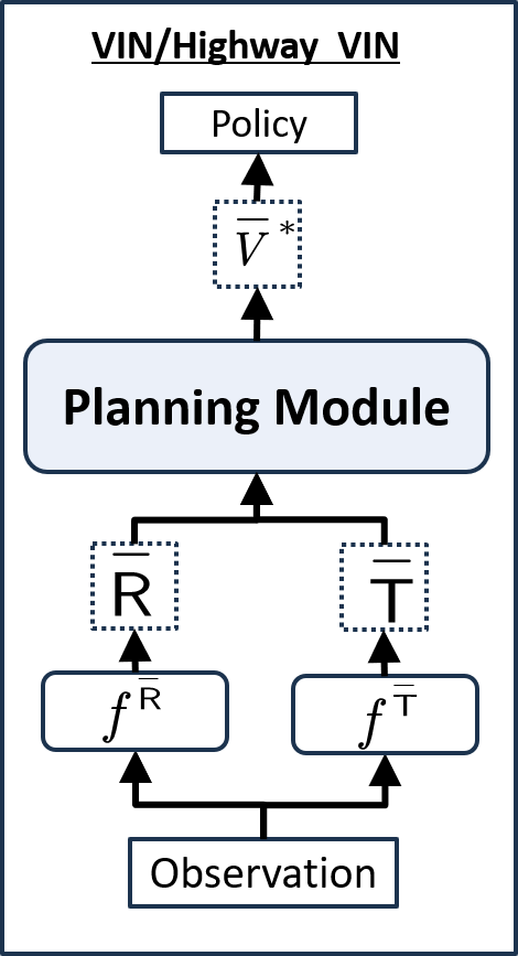
(a)

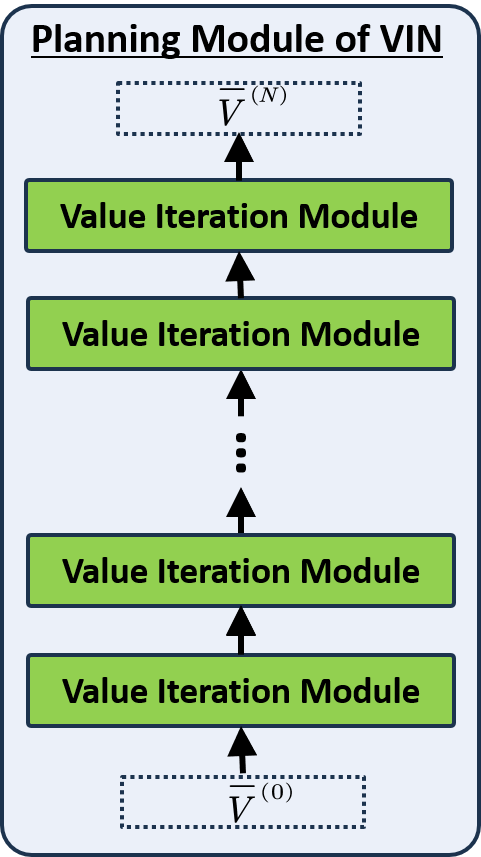
(b)

Figure 2: 2(a): Architecture of VIN and highway VIN. 2(b): Architecture of the planning module of VIN, which includes $N$ layers of value iteration modules. The architecture of the value iteration module is detailed in Fig. 4(a).

Highway Value Iteration.

Highway value iteration (highway VI) is an algorithm derived from the theory of highway RL (Wang et al., 2024), which is a framework for improving the efficiency of long-term credit assignment. This approach introduces a multi-step operator, which averages $n$-step bootstrapping values using various policies, termed lookahead policies, each executed for different $n$ time steps. Here, $n$ represents the lookahead depth. This operator is formally defined as follows:

$${{\mathcal{G}}}_{{{\cal N},\alpha}}^{{{\Pi},\widetilde{\alpha}}}V\triangleq{{\color[rgb]{0,0,0}\underset{\pi\in{\Pi}}{\mathop{smax}\nolimits^{\widetilde{\alpha}}}}{\color[rgb]{0,0,0}\underset{n\in{\cal N}}{\mathop{smax}\nolimits^{\alpha}}}}{\color[rgb]{0.94140625,0,0}\max}\left\{\left(\mathcal{B}^{\pi}\right)^{\circ\left(n-1\right)}\mathcal{B}V,\mathcal{B}V\right\}.$$ (5)

In this formula, ${\Pi}$ denotes the set of lookahead policies and ${\cal N}$ denotes the set of lookahead depths. The softmax function, with a softmax temperature $\alpha$, is defined as: $\underset{x\in\mathcal{X}}{\mathop{smax}\nolimits^{\alpha}}f\left(x\right)\triangleq\sum_{x\in\mathcal{X}}\frac{{\exp\left(\alpha f\left(x\right)\right)}}{\sum_{x^{\prime}\in\mathcal{X}}{\exp\left(\alpha f\left(x^{\prime}\right)\right)}}f\left(x\right).$ Here, $(\cdot)^{\circ k}$ indicates the composition of operator $(\cdot)$ for $k$ times. Based on this operator, the algorithm highway VI iteratively updates the value function as $V^{(n+1)}={{\mathcal{G}}}_{{{\cal N},\alpha}}^{{{\Pi},\widetilde{\alpha}}}V^{(n)}$. Two critical aspects of highway VI are highlighted:

Remark 0.

(Convergence to the Optimal Value Function) The highway VI algorithm is proved to converge to the optimal value function $V^{*}$ regardless of the choice of lookahead policies ${\Pi}$, lookahead depths ${\cal N}$, and softmax temperatures $\tilde{\alpha}$ and $\alpha$. For a detailed formal statement, please refer to their Theorem A.2 (Wang et al., 2024).

Remark 0.

(Importance of the Maximization Operation) The maximization operation, ${\color[rgb]{0.94140625,0,0}\max}\left\{\left(\mathcal{B}^{\pi}\right)^{\circ\left(n-1\right)}\mathcal{B}V,\mathcal{B}V\right\}$, is crucial for ensuring convergence to $V^{*}$. Convergence is not guaranteed without this component. For a detailed formal statement, please refer to their Theorem 1, 2 (Wang et al., 2024).

4 Method

Motivation.

NNs with increased depth have superior representational and generalization capabilities (Szegedy et al., 2014; Ciresan et al., 2011, 2012; Telgarsky, 2016). Building on this knowledge, we propose that increasing the depth of VIN can considerably boost their long-term planning abilities in the context of RL. This proposition is grounded in the intrinsic design of VINs, which includes a value iteration planning module. A theoretical study (see Theorem 1.12, (Agarwal et al., 2019)) indicates that increased iterations in this module can result in a more accurate estimation of the optimal value function, subsequently improving the policy performance.

Overview.

The traditional VIN (Section 3) propagates information layer-by-layer, based on the step-by-step approach of the VI process. The proposed novel method, i.e., highway VINs, enhances VINs by incorporating a distinct planning module inspired by highway VI. As detailed in Section 3, highway VI uses information from various policies and multiple steps ahead, forming a new VIN architecture that facilitates the information flow from various dimensions. The planning module of highway VINs follows the computational process of highway VI in Eq. 5. Below, we detail the transition from the $n$-th activation $\overline{V}^{(n)}$, representative of the iterative process of the proposed planning module.

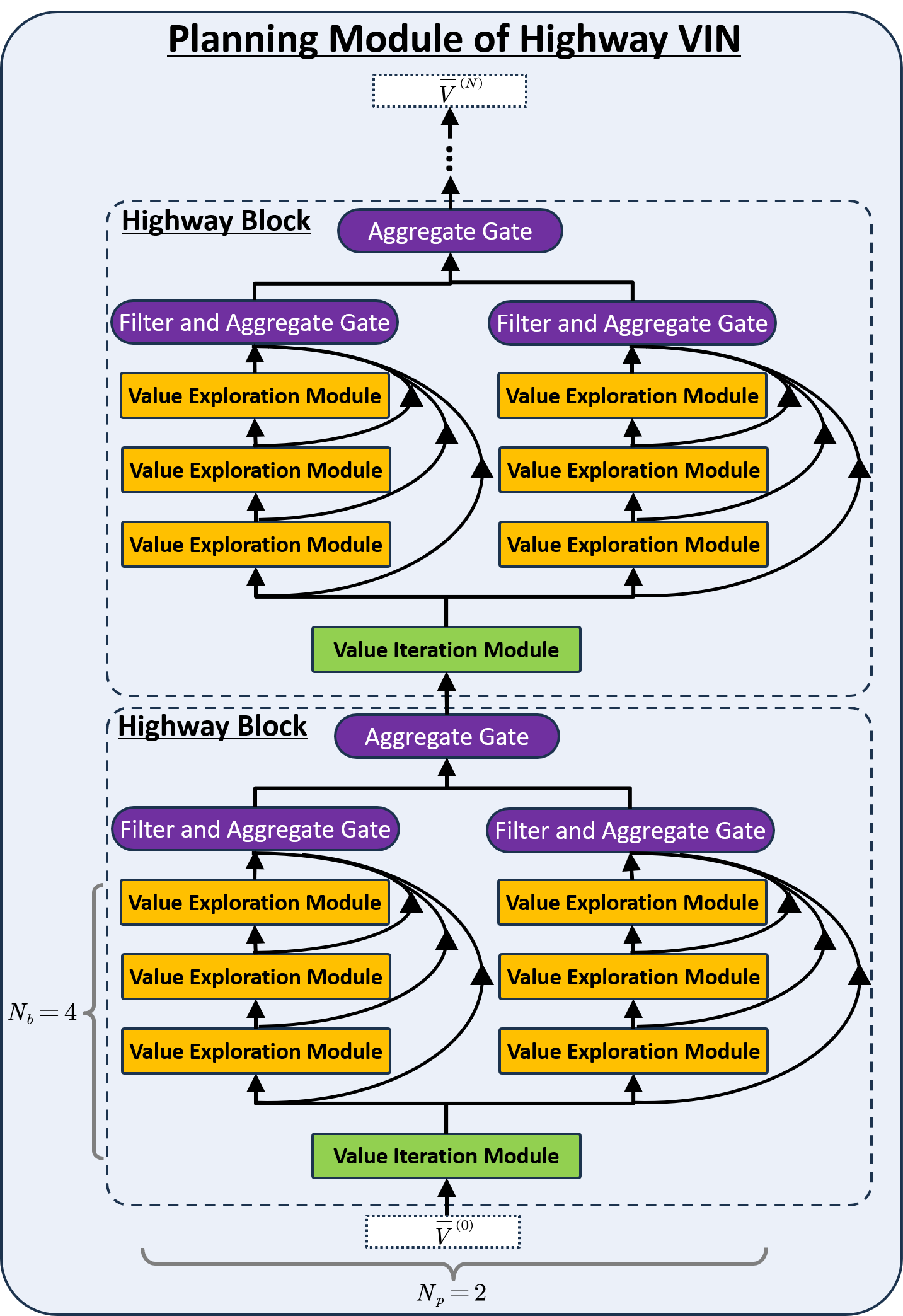
Figure 3: Planning module of highway VIN. Here, we demonstrate the planning module of highway VIN using a highway block of depth $N_{b}=4$ and incorporating $N_{p}=2$ embedded policies.

First, $\overline{V}^{(n)}$ is fed into the value iteration module to generate a new activation $\overline{V}^{(n+1)}$, as in VINs (Eq. 3 and 4). This step corresponds to the Bellman optimality operator $\mathcal{B}(\cdot)$ in highway VI (see Eq. 5).

Then, to facilitate information flow over spatial dimensions, we introduce a new value exploration (VE module) module. Each VE module is equipped with an embedded policy $\overline{\pi}$, defined on the latent MDP $\overline{\mathcal{M}}$ and determining the path of the information flow. Conceptually, it corresponds to one application of the Bellman Expectation operator $\mathcal{B}^{\overline{\pi}}(\cdot)$ in highway VI.

Then, to further facilitate spatial information flow in depth, we stack $N_{p}$ parallel VE modules for $N_{b}-1$ layers, corresponding to multiple compositions $({\mathcal{B}^{\overline{\pi}}})^{\circ(N_{b}-1)}(\cdot)$ in highway VI. These stacked and parallel VE modules process the input $\overline{V}^{(n)}$ , leading to new activations $\{\mathcal{\overline{V}}^{(n+n_{b})}_{n_{p}}\}_{n_{p},n_{b}}$ for various indexes of the parallel modules $n_{p}=1,\cdots,N_{p}$ and various depths $n_{b}=1,\cdots,N_{b}$, where the initial $\mathcal{\overline{V}}_{n_{p}}^{(n+1)}={\overline{V}}^{(n+1)}$ for each $n_{p}$.

Finally, the outputs from these parallel and stacked VE modules are combined using an aggregate gate and a filter gate. This combination forms a skip connection architecture, which eases the training of very deep NNs. These gates mirror the operations ${{\color[rgb]{0,0,0}\underset{\pi}{\mathop{smax}\nolimits^{\widetilde{\alpha}}}}{\color[rgb]{0,0,0}\underset{n}{\mathop{smax}\nolimits^{\alpha}}}}{\color[rgb]{0.94140625,0,0}\max}\{\cdot\}$ in highway VI.

We term the above four procedures as a highway block. The planning module of highway VIN comprises $N_{B}$ such highway blocks. Fig. 3 overviews this planning module. The subsequent sections detail the components of the VE module, filter gate, and aggregate Gate.

4.1 Value Exploration Modules

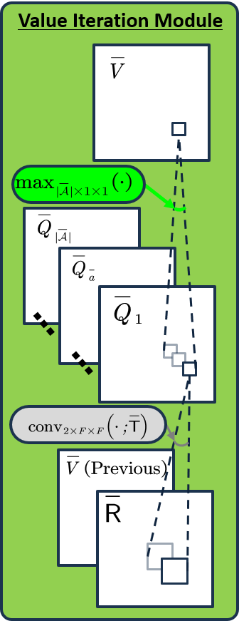
(a)

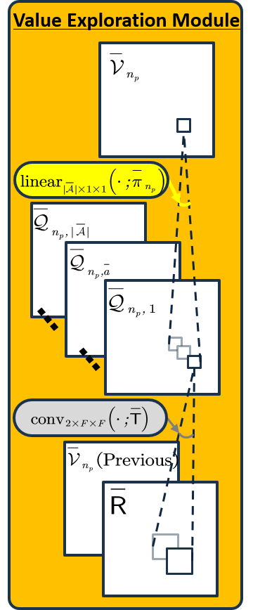
(b)

Figure 4: Architecture of the value iteration module and VE module, respectively. The operation $\max_{\overline{\mathcal{A}}\times 1\times 1}$ denotes a max operation over the action axis, as shown in Eq. 4. The operation $\mathrm{linear}_{\overline{\mathcal{A}}\times 1\times 1}$ represents a linear combination of the input Q matrix $\overline{Q}_{n_{p}}$ and the policy matrix $\overline{\pi}_{n_{p}}$ over the action axis, as shown in Eq. 7.

The value iteration module in VINs greedily takes the largest Q value, as shown in Eq. 4. Consequently, this mechanism can result in a distinctive information flow for each layer, thereby channeling gradients toward certain specific neurons. To facilitate the information and gradient flow across spatial dimensions, we introduce a new VE module. Each VE module is equipped with an embedded policy, which determines the path of the information flow. The VE module computes values according to Bellman expectation operator $\mathcal{B}^{\overline{\pi}}(\cdot)$ in highway VI:

$$\overline{\mathcal{Q}}_{\overline{\pi},\overline{a},i,j}^{(n+n_{b})}=\sum_{i^{\prime},j^{\prime}}{\left(\overline{\mathsf{T}}_{\overline{a},i^{\prime},j^{\prime}}\overline{\mathsf{R}}_{i-i^{\prime},j-j^{\prime}}+\overline{\mathsf{T}}_{\overline{a},i^{\prime},j^{\prime}}\overline{\mathcal{V}}_{\overline{\pi},i-i^{\prime},j-j^{\prime}}^{(n+n_{b}-1)}\right)}$$ (6)

$$\overline{\mathcal{V}}_{n_{p},i,j}^{(n+n_{b})}=\sum_{\overline{a}}{\overline{\pi}_{n_{p},\overline{a},i,j}^{\left(n+n_{b}\right)}\overline{\mathcal{Q}}_{n_{p},\overline{a},i,j}^{(n+n_{b})}}$$ (7)

where ${\overline{\pi}}^{(n+n_{b})}_{n_{p}}\in\mathbb{R}^{|\mathcal{A}|\times m\times m}$ represents the $n_{p}$-th embedded policy for $(n+n_{b})$-th layer. Here, the value functions are denoted as $\mathcal{\overline{V}}$ and $\mathcal{\overline{Q}}$ to distinguish them from the value functions $\overline{V}$ and $\overline{Q}$ of the VI module. As implied by Eq. 7, instead of taking maximization over the actions as in the VI module (see Eq. 4), the proposed VE module takes expectation over actions based on the distribution of the embedded policy ${\overline{\pi}}_{n_{p}}$. The computation process of the VE module is shown in Fig. 4(b).

Note that, as stated in Remark ‣ 3, convergence in highway VI is assured regardless of the chosen lookahead policies. These policies correspond to embedded policies within several VE modules of highway VINs. Generally, the embedded policy can be generated using a learnable mapping function ${\overline{\pi}}^{(n+n_{b})}_{n_{p}}=f^{\overline{\pi}}\left(\mathcal{\overline{Q}}_{n_{p}}^{(n+n_{b})},\phi(s);W^{(n+n_{b})}_{n_{p}}\right)$, where $W^{(n+n_{b})}_{n_{p}}$ are learnable parameters. Drawing inspiration from the dropout technique, which introduces stochasticity into the activations to increase robustness (Srivastava et al., 2014; Hanson, 1990; Hertz et al., 1991; Baldi & Sadowski, 2013), we randomly generate multiple embedded policies as follows:

$${\overline{\pi}}^{(n+n_{b})}_{n_{p},\overline{a},i,j}=\begin{cases}1,&\overline{a}=\widehat{\overline{a}}\sim P\left(\cdot;\mathcal{\overline{Q}}_{n_{p},\cdot,i,j}^{\left(n+n_{b}\right)},\epsilon\right)\\ 0,&\text{otherwise,}\end{cases}$$ (8)

where $\epsilon$ is the embedded exploration rate, and $\widehat{\overline{a}}$ is a sampled action drawn from the $\epsilon$-greedy distribution $P\left(\cdot;\mathcal{\overline{Q}}_{n_{p},\cdot,i,j}^{\left(n+n_{b}\right)},\epsilon\right)$, defined as:

$$P\left(\overline{a};\mathcal{\overline{Q}}_{n_{p},\cdot,i,j}^{\left(n+n_{b}\right)},\epsilon\right)=\begin{cases}1-\epsilon+\frac{\epsilon}{|\mathcal{\overline{A}}|},&\overline{a}=\operatorname*{arg\,max}\limits_{\overline{a}^{\prime}}\mathcal{\overline{Q}}_{n_{p},\overline{a}^{\prime},i,j}^{\left(n+n_{b}\right)}\\ \frac{\epsilon}{|\mathcal{\overline{A}}|},&\mathrm{otherwise.}\end{cases}$$

During the training phase, the embedded policies are generated randomly for each iteration. In contrast, we adopt greedy policies during the evaluation phase, where trained models are applied in realistic environments, defined as follows:

$$\overline{\pi}_{n_{p},\overline{a},i,j}^{\left(n+n_{b}\right)}=\begin{cases}1,&\overline{a}=\mathrm{arg}\max_{\overline{a}^{\prime}}\overline{\mathcal{Q}}_{n_{p},\overline{a}^{\prime},i,j}^{\left(n+n_{b}\right)}\\ 0,&\mathrm{otherwise.}\\ \end{cases}$$

This equation indicates that, during the evaluation phase, VE modules function in the same way as VI modules. In practice, we observe that incorporating this stochastic mechanism substantially improves robustness and is essential for achieving high performance. Moreover, this stochasticity does not impact the convergence to the optimal value function. As stated by the theory of highway VI in Remark , convergence is guaranteed irrespective of any chosen embedded policies, even if they are fully stochastic.

4.2 Aggregate and Filter Gates

We aim to integrate the proven efficacy of skip connections in training very deep NNs (Srivastava et al., 2015b; He et al., 2016). However, theoretically validating this architecture within the RL framework and ensuring its compatibility with the stochasticity in the VE modules are challenging. The highway VI algorithm offers a guiding principle for this design. By implementing the ${{\color[rgb]{0,0,0}\underset{\pi}{\mathop{smax}\nolimits^{\widetilde{\alpha}}}}{\color[rgb]{0,0,0}\underset{n}{\mathop{smax}\nolimits^{\alpha}}}}{\color[rgb]{0.94140625,0,0}\max}\{\cdot\}$ operations of highway VI, the activations are aggregated as follows:

$$\overline{V}_{i,j}^{(n+N_{b})}=\sum_{n_{p}=1}^{N_{p}}{\widetilde{\mathsf{A}}_{n_{p},i,j}^{\left(n+N_{b}\right)}\underset{{\overline{V}^{\prime\prime}}_{n_{p},i,j}^{\left(n+N_{b}\right)}}{\underbrace{\sum_{n_{b}=1}^{N_{b}}{\mathsf{A}_{n_{p},i,j}^{\left(n+n_{b}\right)}\overset{{\overline{V}^{\prime}}_{n_{p},i,j}^{\left(n+n_{b}\right)}}{\overbrace{{\color[rgb]{0.94140625,0,0}\max}\left\{\overline{\mathcal{V}}_{n_{p},i,j}^{\left(n+n_{b}\right)},\overline{V}_{i,j}^{\left(n+1\right)}\right\}.}}}}}}$$

Here, $\widetilde{\mathsf{A}}_{n_{p},i,j}^{\left(n+N_{b}\right)}$ and ${\mathsf{A}}_{n_{p},i,j}^{\left(n+n_{b}\right)}$ are termed as the aggregate gate, reflecting the degree to which activations contribute to the output, similar to the concept in highway networks (Srivastava et al., 2015b, a). The aforementioned equation illustrates the aggregation of activations from various layers across multiple parallel VE modules, i.e., $\left\{\mathcal{\overline{V}}_{n_{p}}^{\left(n+n_{b}\right)}\right\}_{n_{p},n_{b}}$, for $n_{p}=1,\cdots,N_{p}$ and $n_{b}=1,\cdots,N_{b}$. Fig. 3 illustrates the information flow of this computation process. Aggregate gates can be generally generated using mapping functions as follows: ${\mathsf{A}}_{n_{p}}^{\left(n+n_{b}\right)}=f^{{\mathsf{A}}}\left(\left\{\overline{{V}}_{n_{p}}^{(n+n_{b}^{\prime})}\right\}_{n_{b}^{\prime}},\phi(s);U_{n_{p}}^{(n+n_{b})}\right)$. Here, $U^{(n+n_{b})}_{n_{p}}$ are learnable parameters. For simplicity and consistency with highway VI, we use softmax weights in the following form:

$$\widetilde{\mathsf{A}}_{n_{p},i,j}^{\left(n+N_{b}\right)}=\frac{\exp\left(\alpha_{\widetilde{\mathsf{A}}}{\overline{V}^{\prime\prime}}_{n_{p},i,j}^{\left(n+N_{b}\right)}\right)}{\sum\limits_{n_{p}^{\prime}}{\exp\left(\alpha_{\widetilde{\mathsf{A}}}{\overline{V}^{\prime\prime}}_{n_{p}^{\prime},i,j}^{\left(n+N_{b}\right)}\right)}},\text{for various }n_{p},$$

$$\mathsf{A}_{n_{p},i,j}^{\left(n+n_{b}\right)}=\frac{\exp\left(\alpha_{\mathsf{A}}{\overline{V}^{\prime}}_{n_{p},i,j}^{\left(n+n_{b}\right)}\right)}{\sum\limits_{n_{b}^{\prime}}{\exp\left(\alpha_{\mathsf{A}}{\overline{V}^{\prime}}_{n_{p},i,j}^{\left(n+n_{b}^{\prime}\right)}\right)}},\text{for various }n_{b},$$

where $\alpha_{\widetilde{\mathsf{A}}}$ and $\alpha_{\mathsf{A}}$ are the softmax temperatures that vary for each highway block and learnable via backpropagation.

The maximization operation $\color[rgb]{1,0,0}{\max}\{\cdot\}$, which we term filter gate, compares the $(n+n_{b})$-th activation $\mathcal{\overline{V}}_{n_{p}}^{\left(n+n_{b}\right)}$ with the $(n+1)$-th one $\overline{V}^{\left(n+1\right)}$, selecting the maximum value. This filter gate is essential for discarding any activations $\mathcal{\overline{V}}_{n_{p}}^{\left(n+n_{b}\right)}$ that are lower than $\overline{V}^{\left(n+1\right)}$, effectively filtering out explorations in VE modules that do not contribute to convergence. Furthermore, as suggested in Remark , this operation is crucial for ensuring convergence.

4.3 Relation to Highway Networks

Section 4.2 and Fig. 3 illustrate the planning module of highway VIN, which features an architecture with skip connections similar to those found in established NNs such as highway networks (Srivastava et al., 2015b, a) and their variants residual networks (He et al., 2016) and DenseNets (Huang et al., 2017). A straightforward approach is to directly implement skip connections in VINs as follows:

$$\overline{V}_{i,j}^{(n+N_{b})}=\sum_{n_{b}=1}^{N_{b}}{\mathsf{A}_{i,j}^{\left(n+n_{b}\right)}\overline{V}_{i,j}^{\left(n+n_{b}\right)}}.$$ (9)

Here, $\overline{V}_{i,j}^{\left(n+n_{b}\right)}$ is derived from the VI module (Eqs. 3 and 4), using $\overline{V}_{i,j}^{\left(n+n_{b}-1\right)}$ as the input. While this method helps to address optimization challenges in training very deep VINs, it has not shown effectiveness in improving long-term planning capabilities (Table 1 in Section 5). Highway VINs include two additional critical components: a VE module that improves the diversity of information and gradient flow, and an innovative filter gate designed to eliminate useless information generated by the VE modules. This study also reveals the underlying connections between the highway RL and highway networks, which were initially proposed under different contexts and purposes but share fundamental similarities.

Table 1: The success rates for each algorithm with various depths under 2D maze navigation tasks with different ranges of shortest path length. Please also refer to Appendix Table 4 for the results of all the other depths.

Maze Size	$15\times 15$				$25\times 25$
Shortest Path Length		$[1,30]$	$[30,60]$	$[60,100]$		$[1,60]$	$[60,130]$	$[130,230]$
VIN (Tamar et al., 2016)	$N=20$	$99.83\pm 0.11$	$96.48\pm 0.58$	$63.03\pm 3.20$	$N=30$	$98.84\pm 0.16$	$49.25\pm 4.16$	9$2.96\pm 0.66$
	$N=40$	$99.79\pm 0.10$	$95.84\pm 0.69$	$76.16\pm 1.87$	$N=60$	$96.47\pm 1.33$	$48.26\pm 4.21$	9$7.87\pm 3.54$
	$N=100$	9$0.80\pm 0.03$	9$0.00\pm 0.00$	9$0.00\pm 0.00$	$N=150$	9$0.22\pm 0.08$	9$0.00\pm 0.00$	9$0.00\pm 0.00$
	$N=200$	9$0.56\pm 0.00$	9$0.00\pm 0.00$	9$0.00\pm 0.00$	$N=300$	9$0.24\pm 0.00$	9$0.00\pm 0.00$	9$0.00\pm 0.00$
GPPN (Lee et al., 2018)	$N=20$	$99.98\pm 0.01$	$92.68\pm 1.07$	$51.12\pm 5.00$	$N=30$	$98.98\pm 0.25$	$25.98\pm 5.78$	9$2.76\pm 1.68$
	$N=40$	${\color[rgb]{0,0,1}\mathbf{99.99\pm 0.01}}$	$96.16\pm 3.56$	$65.17\pm 12.4$	$N=60$	${\color[rgb]{0,0,1}\mathbf{99.09\pm 0.19}}$	$28.87\pm 1.47$	9$1.32\pm 0.55$
	$N=100$	$99.95\pm 0.05$	$93.34\pm 4.16$	$60.57\pm 13.6$	$N=150$	$98.51\pm 0.31$	$21.62\pm 3.50$	9$0.73\pm 0.68$
	$N=200$	$99.98\pm 0.01$	$92.79\pm 1.28$	$50.88\pm 3.59$	$N=300$	$95.38\pm 2.01$	9$6.29\pm 4.35$	9$0.02\pm 0.03$
Highway network (Srivastava et al., 2015b)	$N=40$	$99.65\pm 0.17$	$96.04\pm 0.63$	$75.86\pm 10.0$	$N=60$	$97.93\pm 0.56$	$62.95\pm 8.79$	$17.46\pm 5.45$
	$N=100$	$99.36\pm 0.32$	$91.11\pm 2.64$	$60.32\pm 8.87$	$N=150$	$85.42\pm 4.20$	$12.55\pm 3.89$	9$0.35\pm 0.23$
	$N=200$	9$0.73\pm 0.12$	9$0.00\pm 0.00$	9$0.00\pm 0.00$	$N=300$	9$0.24\pm 0.00$	9$0.00\pm 0.00$	9$0.00\pm 0.00$
Highway VIN (ours)	$N=40$	$99.77\pm 0.09$	$98.83\pm 0.25$	$90.00\pm 2.12$	$N=60$	$97.87\pm 0.60$	$77.02\pm 6.30$	$20.68\pm 9.89$
	$N=100$	$99.93\pm 0.03$	${\color[rgb]{0,0,1}\mathbf{99.52\pm 0.12}}$	${\color[rgb]{0,0,1}\mathbf{98.61\pm 0.66}}$	$N=150$	$97.77\pm 0.48$	$89.56\pm 0.95$	$75.42\pm 10.1$
	$N=200$	$99.94\pm 0.01$	$99.13\pm 0.12$	$98.20\pm 1.75$	$N=300$	$98.73\pm 0.50$	${\color[rgb]{0,0,1}\mathbf{92.28\pm 3.50}}$	${\color[rgb]{0,0,1}\mathbf{90.06\pm 3.13}}$

5 Experiments

We conduct a series of experiments to evaluate how highway VINs can improve the long-term planning capabilities of VINs for complex tasks. We also explore the significance of each component within the highway VINs.

5.1 2D Maze Navigation

We evaluate the algorithms on 2D maze navigation tasks of various sizes $m\times m$, specifically $15\times 15$ and $25\times 25$. In these tasks, the agent can move forward, turn 90 degrees left or right, and has four orientations. We follow the experimental setup described in the paper on GPPN (Lee et al., 2018). We train the models for $30$ epochs using imitation learning on a labeled training dataset, select the best model based on validation dataset performance, and test it on a separate test dataset. Each dataset contains numerous planning tasks, each involving a maze with a start position, an image of the $m\times m$ map, and a goal position represented by a $4\times m\times m$ matrix (where $4$ corresponds to the four orientations). These datasets involve tasks requiring planning over hundreds of steps to reach the goal. For more detailed information about the dataset, please refer to Appendix A.

We measure the planning abilities of an agent based on the success rate (SR), which is defined as the ratio of the number of successfully completed tasks to the total number of planning tasks. The agent is considered to succeed in a task if it generates a path from the start position to the goal position within a limited number of steps. To assess the planning ability of the algorithms across different scales, we evaluate them on navigation tasks with varying shortest path lengths (SPLs) from start to goal. These lengths are calculated in advance using Dijkstra’s algorithm with access to the maze’s underlying structure. Tasks with longer SPLs typically demand greater long-term planning capabilities. We follow the GPPN paper’s setting, evaluating each algorithm with $3$ random seeds. We report the mean and standard deviation on the test dataset.

Subsequently, we compare the highway VINs against several advanced NNs for planning tasks. The baseline model is the original VIN (Tamar et al., 2016). We also compare highway VINs against GPPNs (Lee et al., 2018), which improve the training stability of VINs using gated recurrent operators such as LSTM updates and the highway networks (Srivastava et al., 2015b), which incorporate skip connections for training of very deep NNs (adapted here for VINs, Section 4.3). We follow the hyperparameter settings listed in the paper on GPPNs (Lee et al., 2018). To ensure a fair comparison, we set the number of parallel VE modules of highway VINs to $N_{p}=1$ unless stated otherwise. The embedded exploration rate is set to $\epsilon=1$ (defined in Eq. 8). Note that this setting does not result in a sub-optimal solution of the latent value function due to the filter gate, which excludes actions detrimental to convergence. The baseline uses a $20$-layer VIN and GPPN for the $15\times 15$ Maze, and a $30$-layer VIN and GPPN for the $25\times 25$ Maze. For both highway networks and highway VINs, we set $N_{B}=20$ highway blocks for the $15\times 15$ maze and $N_{B}=30$ for the $25\times 25$ maze. We set various highway block depths $N_{b}\geq 2$, which yields various total depths: $N=N_{b}*N_{B}$, specifically $N\in\{40,60,80,120,160,200\}$ for the $15\times 15$ maze and $N\in\{60,90,120,150,180,240,300\}$ for the $25\times 25$ maze. The baselines VIN and GPPN are also tested using the same depths.

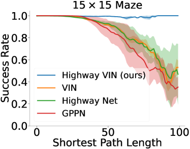
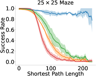
Figure 5: Success rates of the algorithms are presented as a function of varying shortest path length. For each algorithm, the optimal result from a range of depths is selected. For a comprehensive view of the results across all depths, please see Fig. 9 in the Appendix.

(a)

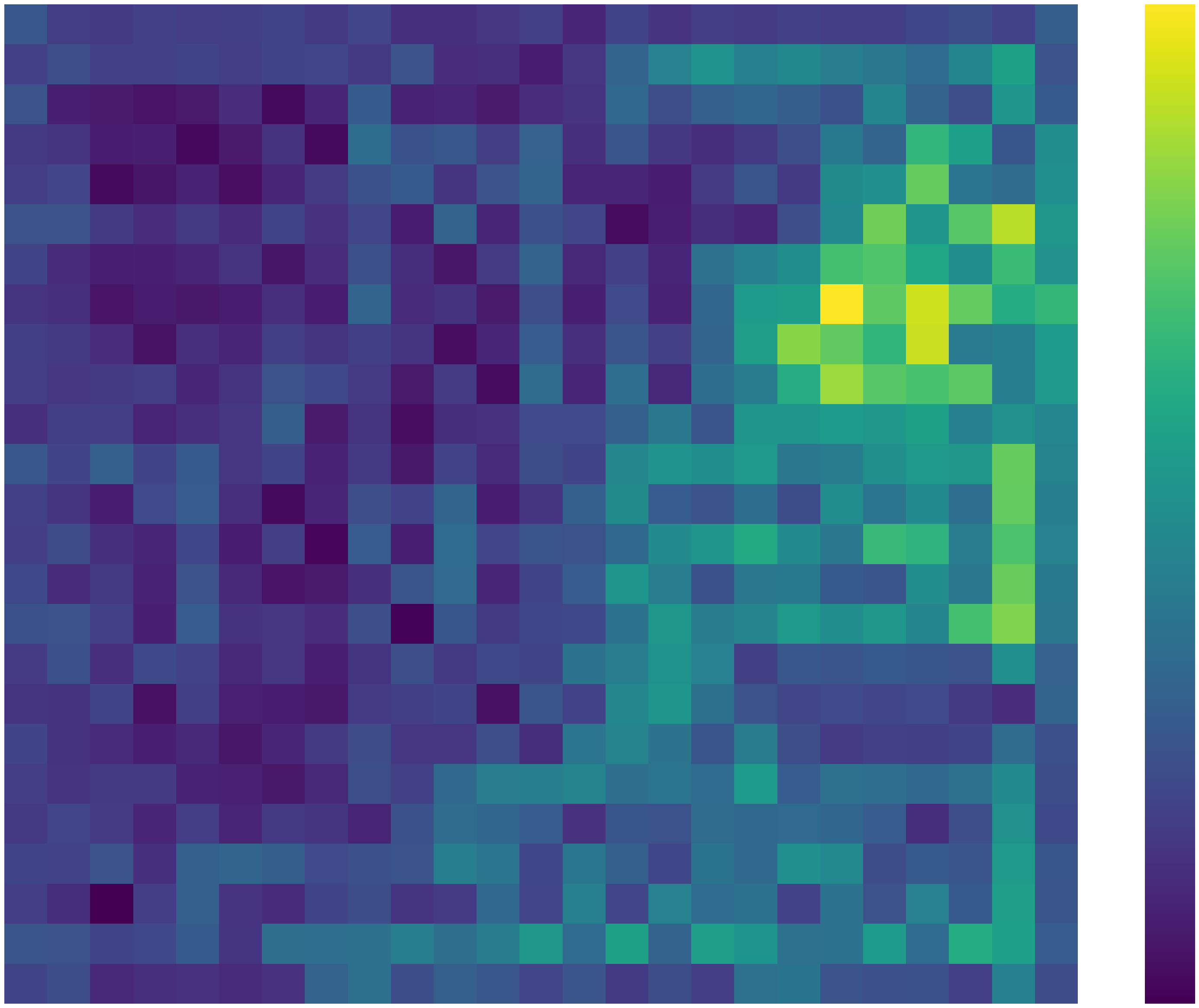
(b)

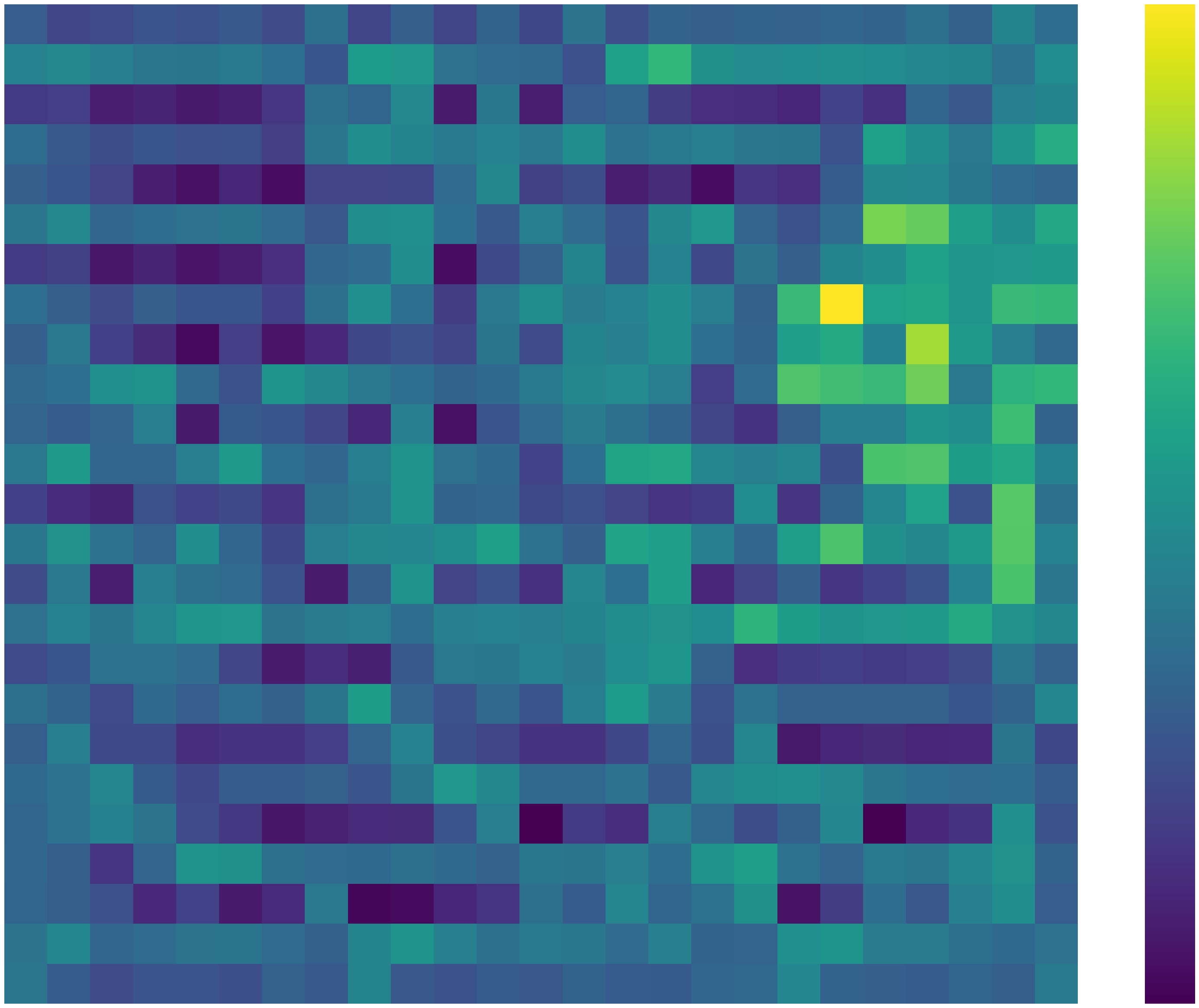
(c)

Figure 6: LABEL:fig_maze An example of $25\times 25$ Maze. LABEL:fig_heatmap_VIN and LABEL:fig_heatmap_HighwayVIN learned feature maps of VIN and highway VIN, respectively.

Peformance with the Best NN Depth.

Fig. 5 shows the SRs of various algorithms under tasks with different SPLs. To ensure a fair comparison, we select the best results from varying NN depths for each algorithm as each algorithm may perform optimally at different depths (please refer to Fig. 9 in Appendix for a comprehensive view of the results across all depths). The results demonstrate that the SRs for all compared methods considerably decrease with increasing SPLs. Remarkably, when the SPL exceeds 200 in the $25\times 25$ Maze, the SRs of all methods nearly drop to 0%. In contrast, highway VIN maintains an impressive 98% SR with an SPL of $100$ in the $15\times 15$ Maze and 90% SR with an SPL of $200$ in the $25\times 25$ Maze.

Additionally, Fig. 6 shows the feature map of the VIN and highway VIN, which can conceptually be understood as the learned value function. The figure reveals that the learned values of highway VIN for states distant from the goal are larger than those of VIN, implying that highway VIN learns an effective value function for long-term planning.

Peformance with Various Depths.

Table 1 shows the SRs of each algorithm across various depths and tasks with different SPL ranges (see Table 4 in the Appendix for results across all depths). The table shows that the highway VINs generally perform better with increased depth. Notably, we observe a +69.38% improvement in the SR of the $25\times 25$ maze with an SPL range of $[130,230]$ as the depth $N$ increases from $60$ to $300$.

The performance of the VIN decreases with increasing depth. Specifically, the SR of VINs drops to nearly 0% for all tasks at a depth of $N>150$. The highway network, in contrast, maintains its performance even at greater depths. However, an increase in depth does not considerably improve its long-term planning capabilities. We hypothesize that integrating the skip connections of highway networks into VINs does not introduce additional architectural inductive bias beneficial for planning.

The GPPN effectively mitigates the challenges of training very deep models and performs robustly across various depths. In particular, the GPPN excels in tasks with short SPLs, achieving a 99.09% SR on a $25\times 25$ maze with an SPL range of $[1,30]$. However, the GPPN does not show a notable improvement in long-term planning capabilities with an increased depth. For instance, the SR of the GPPN drops to less than 3% on a $25\times 25$ maze with an SPL range of $[130,230]$. This might be because the GPPN, as a black box method with less inductive bias towards planning, is more suited to learning patterns for short-term planning tasks rather than those requiring long-term planning skills.

5.2 Ablation Study

Several ablation studies were conducted to evaluate: 1) the effectiveness of the filter gate (Section 4.2); 2) the impact of the VE module (Section 4.1). We also evaluate the influence of the number of parallel VE modules in Section B.2. In the highway VIN experiments, the default hyperparameters include an exploration rate $\epsilon$ of 1, a single parallel VE module ($N_{p}=1$), and depth configurations of 200 for the $15\times 15$ mazes and 300 for the $25\times 25$ mazes.

Filter Gate.

The SRs of highway VINs, with and without the filter gate, are shown in Fig. 7. The performance considerably decreases when the filter gate is absent. This is because, without a filter gate, highway VINs could easily suffer the adverse effects of exploration in VE modules, which could prevent convergence.

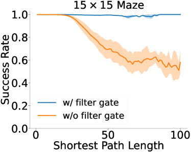
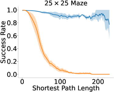
Figure 7: Success rates of highway VIN with and without the filter gate.

VE Modules.

We also evaluate a variant of highway VIN without the VE module (referred to as w/o VE modules), which means that all VE modules are replaced with VI modules. Fig. 8 shows the SRs for the variants with and without the VE module. Without VE modules, the performance of highway VINs notably diminishes in the $25\times 25$ maze. In comparison, the variant equipped with the VE modules performs much better. This improvement is likely due to the use of diverse latent actions, which could facilitate information flow among various neurons in the NN. Table 2 lists the entropy of the selected latent actions of VIN and highway VIN. For VIN, it always selects the action that leads to the maximum Q value. Although the selected latent actions generally vary for each layer because the Q values dynamically change for each layer, they will converge to the same actions when the Q values converge. Therefore, the diversity of the selected actions for VIN is much more limited. Instead, in the proposed highway VIN, we employ the value exploration module to maintain diversity.

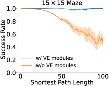
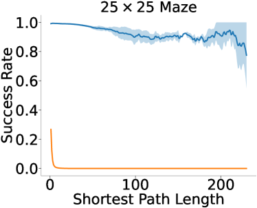
Figure 8: Success rates of highway VIN with and without the VE modules,

Table 2: The entropy of the selected latent actions of VIN and highway VIN with various depths. The entropy is computed by $\sum_{\overline{a}\in\overline{\mathcal{A}}}{\left[-p(\overline{a})\log p(\overline{a})\right]}$, where $p(\overline{a})=\frac{\mathrm{cnt}(\overline{a})}{\sum_{\overline{a}\in\overline{\mathcal{A}}}{\mathrm{cnt}{(\overline{a})}}}$ and $\mathrm{cnt}(\overline{a})$ is the number of selected latent actions equals to $\overline{a}$ over the latent actions across all hidden layers.

Maze Size	$15\times 15$			$25\times 25$
Depth	$40$	$100$	$200$	$60$	$150$	$300$
VIN	0.51	0.14	0.00	0.63	0.07	0.00
Highway VIN (ours)	2.04	3.53	4.17	2.27	3.77	4.35

5.3 3D ViZDoom Navigation

We evaluate the proposed approach in 3D ViZDoom environments (Wydmuch et al., 2019). Following the experimental setting of the GPPN paper (Lee et al., 2018), the input to the model consists of RGB images capturing the first-person view, rather than the top-down 2D maze. Based on these observations, a CNN is employed to predict the maze map, which is then inputted into the planning model (such as VIN or highway VIN), using an architecture and hyperparameters similar to the 2D maze setup. We select the optimal depth from $N=40,100,200$ for each algorithm. Highway VIN performs optimally at depth $100$, while other methods perform best at depth $40$. Table 3 shows the SRs in $15\times 15$ 3D ViZDoom maze navigation. Our highway VINs excel in tasks with SPLs exceeding 30.

Table 3: Success rates of each algorithm with various depths under 3D ViZDoom maze navigation tasks with different ranges of SPLs.

	$[1,30]$	$[30,60]$	[60,100]
VIN	$98.57\pm 1.54$	$92.03\pm 2.03$	$69.37\pm 2.63$
GPPN	${\color[rgb]{0,0,1}{\mathbf{99.91\pm 0.10}}}$	$89.95\pm 9.21$	$44.42\pm 8.14$
Highway network	$97.82\pm 1.01$	$91.99\pm 2.54$	$63.78\pm 11.49$
Highway VIN (ours)	$99.43\pm 0.18$	${\color[rgb]{0,0,1}{\mathbf{98.70\pm 0.38}}}$	${\color[rgb]{0,0,1}{\mathbf{96.98\pm 1.20}}}$

5.4 Computational Complexity

The proposed approach introduces a minimal number of additional parameters to the existing VIN architecture, specifically the softmax temperatures for each highway block denoted as $\{(\alpha_{\widetilde{A}}^{(n_{B})},\alpha_{A}^{(n_{B})})\}_{n_{B}=1}^{N_{B}}$. Note that $N_{B}$ indicates the total number of highway blocks, which are set to $N_{B}=20$ for the $15\times 15$ maze and $N_{B}=30$ for the $25\times 25$ maze. Additionally, the following table details the GPU memory consumption and training duration for each method when employing $300$ layers on NVIDIA A100 GPUs.

	VIN	GPPN	Highway network	Highway VIN (ours)
GPU Memory	3.1G	103.0G	3.3G	15.0G
Training Time	7.5 hours	6.5 hours	7.7 hours	9.0 hours

6 Conclusions

This paper presents a general framework based on highway RL to improve the long-term planning ability of VINs. We improve traditional VINs by incorporating three key components: an aggregate gate, which establishes skip connections and facilitates long-term credit assignment; an exploration module, crafted to diversify information and gradient flow between neurons; and a filter gate, designed to eliminate non-essential information. Our experiments demonstrate that highway VINs enable long-term planning by training neural networks with hundreds of layers, surpassing the performance of several advanced methods. Future research will investigate the integration of multiple parallel VE modules with various types of embedded policies to improve performance. Additionally, future work will focus on scaling up to larger tasks.

Impact Statement

This paper introduces research aimed at advancing the field of machine learning. While acknowledging numerous potential societal consequences, we believe that none need to be specifically emphasized here.

Appendix A Experimental Details

Our experimental settings follow those outlined in the paper on GPPN (Lee et al., 2018). For maze navigation tasks, the training, validation, and test datasets comprise $25K$, $5K$, and $5K$ mazes, respectively.

All models are trained for $30$ epochs using the RMSprop optimizer with a learning rate of $0.001$ and a batch size of $32$. We also specify a kernel size of $5$ for convolutional operations in the planning module, as mentioned in Eq. 3. For the neural network that maps the observation to the latent MDP, we set the hidden dimension to $150$.

Appendix B Additional Experimental Results

B.1 Various Depths of Highway VIN

Table 4 and Fig. 9 show the SRs of various algorithms across different depths. For each algorithm, we also provide the rate at which it can plan the optimal path that yields the shortest path length, summarized in Table 5.

B.2 Number of Parallel VE Modules

We evaluate highway VIN with varying numbers of parallel VE modules $N_{p}$ under varying depths $N$. As shown in Fig. 10, under different depths $N$, the number of parallel VE modules has a different effect on the performance of highway VIN. For example, under depth $N=300$, with fewer parallel VE modules, i.e., $N_{p}=1$, highway VIN performs the best. While under depth $N=100$, with more VE modules, $N_{p}=3$, highway VIN performs the best. These results imply that the additional parallel VE modules may be detrimental to the performance of very deep networks.

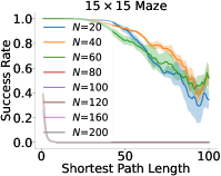
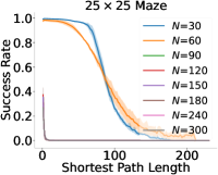
(a)

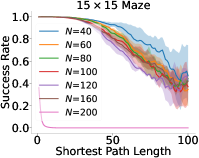
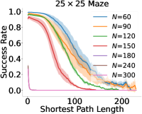
(b)

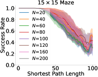
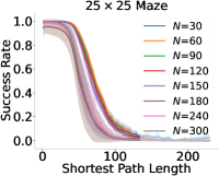
(c)

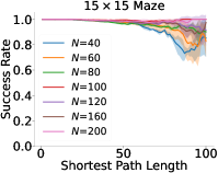
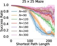
(d)

Figure 9: Success rates of each algorithm as a function of varying shortest path lengths on 2D maze navigation tasks.

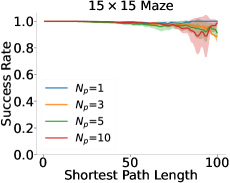
(a)

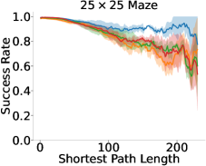
(b)

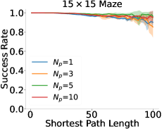
(c)

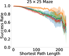
(d)

Figure 10: Success rates of highway VINs with varying numbers of parallel VE modules $N_{p}$ under varying depths $N$ of the network.

B.3 Examples of 2D Maze Navigation

In Fig. 11, we show examples where highway VIN succeeds, but other methods fail.

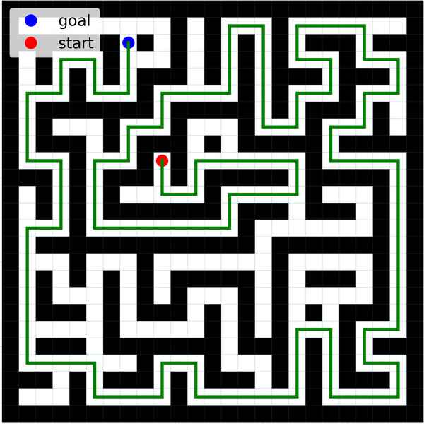
(a)

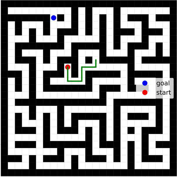
(b)

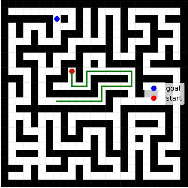
(c)

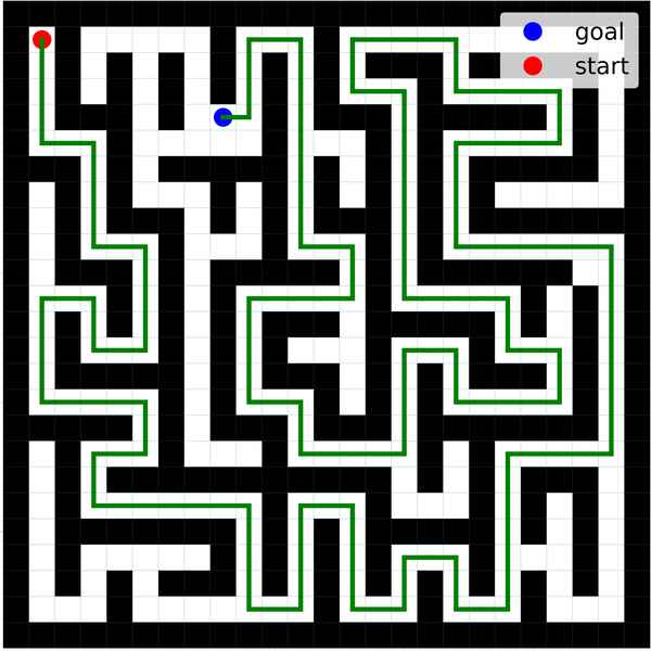
(d)

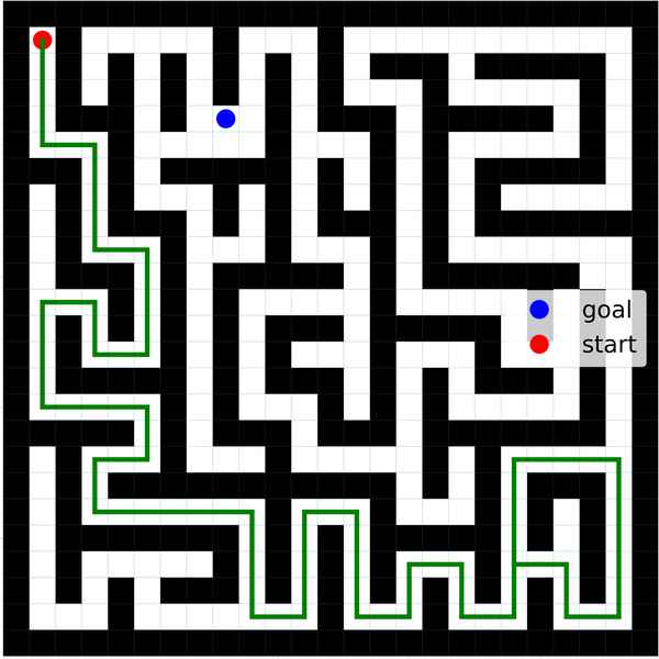
(e)

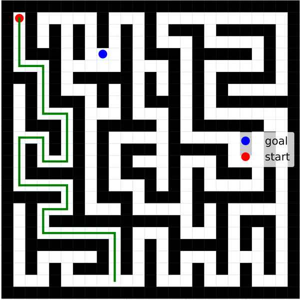
(f)

Figure 11: Examples of 2D maze navigation tasks where highway VIN succeeds, but other methods fail.

Table 4: Success rates of each algorithm with various depths under 2D maze navigation tasks with different ranges of shortest path lengths.

Maze Size	$15\times 15$				$25\times 25$
Shortest Path Length		$[1,30]$	$[30,60]$	$[60,100]$		$[1,60]$	$[60,130]$	$[130,230]$
VIN (Tamar et al., 2016)	$N=20$	$99.83\pm 0.11$	$96.48\pm 0.58$	$63.03\pm 3.20$	$N=30$	$98.84\pm 0.16$	$49.25\pm 4.16$	9$2.96\pm 0.66$
	$N=40$	$99.79\pm 0.10$	$95.84\pm 0.69$	$76.16\pm 1.87$	$N=60$	$96.47\pm 1.33$	$48.26\pm 4.21$	9$7.87\pm 3.54$
	$N=60$	$99.83\pm 0.03$	$92.53\pm 1.33$	$66.18\pm 6.91$	$N=90$	9$0.21\pm 0.08$	9$0.00\pm 0.00$	9$0.00\pm 0.00$
	$N=80$	9$0.65\pm 0.16$	9$0.00\pm 0.00$	9$0.00\pm 0.00$	$N=120$	9$0.21\pm 0.08$	9$0.00\pm 0.00$	9$0.00\pm 0.00$
	$N=100$	9$0.80\pm 0.03$	9$0.00\pm 0.00$	9$0.00\pm 0.00$	$N=150$	9$0.22\pm 0.08$	9$0.00\pm 0.00$	9$0.00\pm 0.00$
	$N=120$	9$0.80\pm 0.03$	9$0.00\pm 0.00$	9$0.00\pm 0.00$	$N=180$	9$0.24\pm 0.00$	9$0.00\pm 0.00$	9$0.00\pm 0.00$
	$N=160$	9$0.64\pm 0.12$	9$0.00\pm 0.00$	9$0.00\pm 0.00$	$N=240$	9$0.24\pm 0.00$	9$0.00\pm 0.00$	9$0.00\pm 0.00$
	$N=200$	9$0.56\pm 0.00$	9$0.00\pm 0.00$	9$0.00\pm 0.00$	$N=300$	9$0.24\pm 0.00$	9$0.00\pm 0.00$	9$0.00\pm 0.00$
GPPN (Lee et al., 2018)	$N=20$	$99.98\pm 0.01$	$92.68\pm 1.07$	$51.12\pm 5.00$	$N=30$	$98.98\pm 0.25$	$25.98\pm 5.78$	9$2.76\pm 1.68$
	$N=40$	${\color[rgb]{0,0,1}\mathbf{99.99\pm 0.01}}$	$96.16\pm 3.56$	$65.17\pm 12.4$	$N=60$	${\color[rgb]{0,0,1}\mathbf{99.09\pm 0.19}}$	$28.87\pm 1.47$	9$1.32\pm 0.55$
	$N=60$	$99.96\pm 0.02$	$91.47\pm 3.50$	$54.52\pm 7.32$	$N=90$	$98.59\pm 0.06$	$25.35\pm 2.66$	9$0.86\pm 0.59$
	$N=80$	$99.97\pm 0.03$	$95.44\pm 4.48$	$66.85\pm 15.5$	$N=120$	$98.67\pm 0.37$	$25.60\pm 4.87$	9$1.35\pm 0.98$
	$N=100$	$99.95\pm 0.05$	$93.34\pm 4.16$	$60.57\pm 13.6$	$N=150$	$98.51\pm 0.31$	$21.62\pm 3.50$	9$0.73\pm 0.68$
	$N=120$	${\color[rgb]{0,0,1}\mathbf{99.99\pm 0.01}}$	$95.57\pm 3.27$	$66.99\pm 15.2$	$N=180$	$90.49\pm 8.62$	9$7.40\pm 8.56$	9$0.41\pm 0.58$
	$N=160$	$99.96\pm 0.01$	$95.51\pm 3.13$	$66.74\pm 12.8$	$N=240$	$93.98\pm 2.48$	9$8.64\pm 5.21$	9$0.15\pm 0.11$
	$N=200$	$99.98\pm 0.01$	$92.79\pm 1.28$	$50.88\pm 3.59$	$N=300$	$95.38\pm 2.01$	9$6.29\pm 4.35$	9$0.02\pm 0.03$
Highway network (Srivastava et al., 2015b)	$N=40$	$99.65\pm 0.17$	$96.04\pm 0.63$	$75.86\pm 10.0$	$N=60$	$97.93\pm 0.56$	$62.95\pm 8.79$	$17.46\pm 5.45$
	$N=60$	$99.69\pm 0.11$	$94.31\pm 0.55$	$64.94\pm 5.61$	$N=90$	$94.59\pm 1.51$	$49.91\pm 11.8$	$13.98\pm 5.86$
	$N=80$	$99.70\pm 0.05$	$93.50\pm 1.15$	$62.22\pm 5.87$	$N=120$	$93.65\pm 0.81$	$38.79\pm 2.68$	9$4.05\pm 0.61$
	$N=100$	$99.36\pm 0.32$	$91.11\pm 2.64$	$60.32\pm 8.87$	$N=150$	$85.42\pm 4.20$	$12.55\pm 3.89$	9$0.35\pm 0.23$
	$N=120$	$99.51\pm 0.17$	$88.45\pm 2.60$	$51.88\pm 4.24$	$N=180$	9$0.23\pm 0.01$	9$0.00\pm 0.00$	9$0.00\pm 0.00$
	$N=160$	$99.50\pm 0.05$	$90.11\pm 0.93$	$60.57\pm 3.33$	$N=240$	9$0.25\pm 0.04$	9$0.00\pm 0.00$	9$0.00\pm 0.00$
	$N=200$	9$0.73\pm 0.12$	9$0.00\pm 0.00$	9$0.00\pm 0.00$	$N=300$	9$0.24\pm 0.00$	9$0.00\pm 0.00$	9$0.00\pm 0.00$
Highway VIN (ours)	$N=40$	$99.77\pm 0.09$	$98.83\pm 0.25$	$90.00\pm 2.12$	$N=60$	$97.87\pm 0.60$	$77.02\pm 6.30$	$20.68\pm 9.89$
	$N=60$	$99.83\pm 0.10$	$98.53\pm 0.72$	$94.35\pm 4.15$	$N=90$	$95.31\pm 1.69$	$80.57\pm 7.40$	$34.72\pm 6.27$
	$N=80$	$99.76\pm 0.02$	$98.03\pm 0.02$	$94.79\pm 0.67$	$N=120$	$96.37\pm 1.82$	$84.81\pm 2.12$	$61.09\pm 3.50$
	$N=100$	$99.93\pm 0.03$	${\color[rgb]{0,0,1}\mathbf{99.52\pm 0.12}}$	${\color[rgb]{0,0,1}\mathbf{98.61\pm 0.66}}$	$N=150$	$97.77\pm 0.48$	$89.56\pm 0.95$	$75.42\pm 10.1$
	$N=120$	$99.88\pm 0.04$	$98.62\pm 0.35$	$96.72\pm 1.76$	$N=180$	$95.99\pm 1.75$	$85.18\pm 2.28$	$75.40\pm 4.05$
	$N=160$	$99.86\pm 0.04$	$98.81\pm 0.24$	$96.76\pm 1.02$	$N=240$	$97.64\pm 1.49$	$90.12\pm 3.68$	$82.40\pm 8.95$
	$N=200$	$99.94\pm 0.01$	$99.13\pm 0.12$	$98.20\pm 1.75$	$N=300$	$98.73\pm 0.50$	${\color[rgb]{0,0,1}\mathbf{92.28\pm 3.50}}$	${\color[rgb]{0,0,1}\mathbf{90.06\pm 3.13}}$

Table 5: Optimality rates of each algorithm with various depths under 2D maze navigation tasks with different ranges of shortest path lengths. The optimality rate is defined by the ratio of tasks completed within the steps of the shortest path length to the total number of tasks.

Maze Size	$15\times 15$				$25\times 25$
Shortest Path Length		$[1,30]$	$[30,60]$	$[60,100]$		$[1,60]$	$[60,130]$	$[130,230]$
VIN (Tamar et al., 2016)	$N=20$	$99.15\pm 0.20$	$90.50\pm 0.59$	$53.31\pm 2.28$	$N=30$	$93.94\pm 0.33$	$38.32\pm 3.64$	9$2.25\pm 0.35$
	$N=40$	$98.54\pm 0.13$	$86.71\pm 0.56$	$69.49\pm 2.77$	$N=60$	$88.64\pm 2.81$	$33.74\pm 3.27$	9$6.16\pm 2.38$
	$N=60$	$98.29\pm 0.23$	$81.58\pm 2.57$	$61.12\pm 6.42$	$N=90$	9$0.20\pm 0.09$	9$0.00\pm 0.00$	9$0.00\pm 0.00$
	$N=80$	9$0.61\pm 0.16$	9$0.00\pm 0.00$	9$0.00\pm 0.00$	$N=120$	9$0.20\pm 0.09$	9$0.00\pm 0.00$	9$0.00\pm 0.00$
	$N=100$	9$0.72\pm 0.06$	9$0.00\pm 0.00$	9$0.00\pm 0.00$	$N=150$	9$0.21\pm 0.09$	9$0.00\pm 0.00$	9$0.00\pm 0.00$
	$N=120$	9$0.72\pm 0.06$	9$0.00\pm 0.00$	9$0.00\pm 0.00$	$N=180$	9$0.24\pm 0.00$	9$0.00\pm 0.00$	9$0.00\pm 0.00$
	$N=160$	9$0.58\pm 0.04$	9$0.00\pm 0.00$	9$0.00\pm 0.00$	$N=240$	9$0.24\pm 0.00$	9$0.00\pm 0.00$	9$0.00\pm 0.00$
	$N=200$	9$0.56\pm 0.00$	9$0.00\pm 0.00$	9$0.00\pm 0.00$	$N=300$	9$0.24\pm 0.00$	9$0.00\pm 0.00$	9$0.00\pm 0.00$
GPPN (Lee et al., 2018)	$N=20$	$99.35\pm 0.12$	$83.42\pm 2.24$	$46.97\pm 5.81$	$N=30$	$96.33\pm 0.33$	$19.94\pm 4.66$	9$2.46\pm 1.50$
	$N=40$	${\color[rgb]{0,0,1}\mathbf{99.64\pm 0.16}}$	$90.47\pm 6.65$	$62.09\pm 12.1$	$N=60$	${\color[rgb]{0,0,1}\mathbf{96.53\pm 0.65}}$	$21.20\pm 1.05$	9$1.01\pm 0.58$
	$N=60$	$99.36\pm 0.18$	$82.08\pm 4.75$	$49.27\pm 7.18$	$N=90$	$94.78\pm 0.21$	$17.96\pm 2.25$	9$0.66\pm 0.66$
	$N=80$	$99.41\pm 0.24$	$88.89\pm 7.41$	$61.21\pm 13.3$	$N=120$	$95.44\pm 0.38$	$18.97\pm 3.67$	9$1.22\pm 0.89$
	$N=100$	$99.27\pm 0.27$	$84.47\pm 5.51$	$55.82\pm 12.6$	$N=150$	$95.05\pm 0.66$	$15.52\pm 2.88$	9$0.70\pm 0.65$
	$N=120$	$99.48\pm 0.12$	$88.22\pm 4.97$	$64.14\pm 14.6$	$N=180$	$82.70\pm 11.6$	9$5.40\pm 6.49$	9$0.40\pm 0.56$
	$N=160$	$99.26\pm 0.19$	$85.70\pm 3.63$	$60.75\pm 11.1$	$N=240$	$87.76\pm 3.64$	9$5.82\pm 3.55$	9$0.12\pm 0.08$
	$N=200$	$99.38\pm 0.08$	$84.65\pm 2.02$	$47.10\pm 3.90$	$N=300$	$88.50\pm 4.61$	9$4.10\pm 2.93$	9$0.02\pm 0.03$
Highway network (Srivastava et al., 2015b)	$N=40$	$98.98\pm 0.12$	$89.37\pm 0.73$	$71.27\pm 9.95$	$N=60$	$92.57\pm 1.68$	$46.95\pm 6.95$	$13.72\pm 4.40$
	$N=60$	$98.85\pm 0.06$	$85.92\pm 0.31$	$59.57\pm 6.76$	$N=90$	$85.25\pm 3.39$	$35.28\pm 9.05$	$10.88\pm 4.04$
	$N=80$	$98.62\pm 0.19$	$83.36\pm 0.17$	$56.04\pm 4.09$	$N=120$	$83.27\pm 0.19$	$26.71\pm 2.02$	9$2.48\pm 0.57$
	$N=100$	$97.88\pm 0.24$	$80.06\pm 3.08$	$55.21\pm 9.75$	$N=150$	$71.57\pm 5.70$	9$7.47\pm 2.58$	9$0.10\pm 0.10$
	$N=120$	$97.89\pm 0.33$	$78.04\pm 2.05$	$46.05\pm 4.48$	$N=180$	9$0.23\pm 0.01$	9$0.00\pm 0.00$	9$0.00\pm 0.00$
	$N=160$	$97.88\pm 0.42$	$78.57\pm 0.95$	$54.11\pm 3.72$	$N=240$	9$0.25\pm 0.04$	9$0.00\pm 0.00$	9$0.00\pm 0.00$
	$N=200$	9$0.65\pm 0.09$	9$0.00\pm 0.00$	9$0.00\pm 0.00$	$N=300$	9$0.24\pm 0.00$	9$0.00\pm 0.00$	9$0.00\pm 0.00$
Highway VIN (ours)	$N=40$	$98.78\pm 0.04$	${\color[rgb]{0,0,1}\mathbf{92.81\pm 0.74}}$	$85.49\pm 2.83$	$N=60$	$93.47\pm 0.67$	$62.70\pm 7.87$	$17.15\pm 8.31$
	$N=60$	$98.47\pm 0.12$	$91.46\pm 1.55$	$88.67\pm 3.33$	$N=90$	$89.72\pm 2.16$	$63.87\pm 8.26$	$27.84\pm 5.12$
	$N=80$	$98.62\pm 0.23$	$91.29\pm 0.50$	$90.99\pm 0.41$	$N=120$	$90.41\pm 1.76$	$64.20\pm 0.79$	$49.63\pm 2.57$
	$N=100$	$98.43\pm 0.05$	$90.67\pm 0.51$	${\color[rgb]{0,0,1}\mathbf{94.64\pm 1.61}}$	$N=150$	$92.00\pm 0.58$	$71.91\pm 2.37$	$64.70\pm 9.88$
	$N=120$	$98.37\pm 0.16$	$90.24\pm 1.31$	$93.16\pm 3.63$	$N=180$	$90.65\pm 1.93$	$66.42\pm 1.83$	$66.25\pm 2.94$
	$N=160$	$98.30\pm 0.11$	$89.15\pm 1.30$	$92.00\pm 0.44$	$N=240$	$91.32\pm 2.24$	$70.78\pm 4.28$	$71.09\pm 8.04$
	$N=200$	$98.26\pm 0.10$	$89.33\pm 0.92$	$92.76\pm 2.08$	$N=300$	$93.36\pm 1.85$	${\color[rgb]{0,0,1}\mathbf{73.35\pm 4.15}}$	${\color[rgb]{0,0,1}\mathbf{81.08\pm 2.87}}$

References

- Agarwal et al. (2019) Agarwal, A., Jiang, N., Kakade, S. M., and Sun, W. Reinforcement learning: Theory and algorithms. CS Dept., UW Seattle, Seattle, WA, USA, Tech. Rep, 32, 2019.
- Baldi & Sadowski (2013) Baldi, P. and Sadowski, P. J. Understanding dropout. Advances in neural information processing systems, 26, 2013.
- Bellman (1966) Bellman, R. Dynamic programming. Science, 153(3731):34–37, 1966.
- Ciresan et al. (2010) Ciresan, D. C., Meier, U., Gambardella, L. M., and Schmidhuber, J. Deep big simple neural nets for handwritten digit recogntion. Neural Computation, 22(12):3207–3220, 2010.
- Ciresan et al. (2011) Ciresan, D. C., Meier, U., Masci, J., Gambardella, L. M., and Schmidhuber, J. Flexible, high performance convolutional neural networks for image classification. In Intl. Joint Conference on Artificial Intelligence IJCAI, pp. 1237–1242, 2011.
- Ciresan et al. (2012) Ciresan, D. C., Meier, U., Masci, J., and Schmidhuber, J. Multi-column deep neural network for traffic sign classification. Neural Networks, 32:333–338, 2012.
- Gers et al. (2000) Gers, F. A., Schmidhuber, J., and Cummins, F. Learning to forget: Continual prediction with LSTM. Neural Computation, 12(10):2451–2471, 2000.
- Hanson (1990) Hanson, S. J. A stochastic version of the delta rule. Physica D: Nonlinear Phenomena, 42(1):265–272, 1990.
- He et al. (2016) He, K., Zhang, X., Ren, S., and Sun, J. Deep residual learning for image recognition. In Proceedings of the IEEE conference on computer vision and pattern recognition, pp. 770–778, 2016.
- Hertz et al. (1991) Hertz, J., Krogh, A., and Palmer, R. Introduction to the Theory of Neural Computation. Addison-Wesley, Redwood City, 1991.
- Hochreiter (1991) Hochreiter, S. Untersuchungen zu dynamischen neuronalen Netzen. Diploma thesis, Institut für Informatik, Lehrstuhl Prof. Brauer, Technische Universität München, 1991. Advisor: J. Schmidhuber.
- Hochreiter & Schmidhuber (1997) Hochreiter, S. and Schmidhuber, J. Long Short-Term Memory. Neural Computation, 9(8):1735–1780, 1997.
- Huang et al. (2017) Huang, G., Liu, Z., Van Der Maaten, L., and Weinberger, K. Q. Densely connected convolutional networks. In Proceedings of the IEEE conference on computer vision and pattern recognition, pp. 4700–4708, 2017.
- Ivakhnenko & Lapa (1965) Ivakhnenko, A. G. and Lapa, V. G. Cybernetic Predicting Devices. CCM Information Corporation, 1965.
- Jin et al. (2021) Jin, X., Lan, W., Wang, T., and Yu, P. Value iteration networks with double estimator for planetary rover path planning. Sensors, 21(24):8418, 2021.
- Lee et al. (2018) Lee, L., Parisotto, E., Chaplot, D. S., Xing, E., and Salakhutdinov, R. Gated path planning networks. In International Conference on Machine Learning, pp. 2947–2955. PMLR, 2018.
- Li et al. (2019) Li, G., Muller, M., Thabet, A., and Ghanem, B. Deepgcns: Can gcns go as deep as cnns? In Proceedings of the IEEE/CVF international conference on computer vision, pp. 9267–9276, 2019.
- Li et al. (2021a) Li, G., Müller, M., Ghanem, B., and Koltun, V. Training graph neural networks with 1000 layers. In International conference on machine learning, pp. 6437–6449. PMLR, 2021a.
- Li et al. (2021b) Li, W., Yang, B., Song, G., and Jiang, X. Dynamic value iteration networks for the planning of rapidly changing uav swarms. Frontiers of Information Technology & Electronic Engineering, 22(5):687–696, 2021b.
- Pflueger et al. (2019) Pflueger, M., Agha, A., and Sukhatme, G. S. Rover-irl: Inverse reinforcement learning with soft value iteration networks for planetary rover path planning. IEEE Robotics and Automation Letters, 4(2):1387–1394, 2019.
- Puterman (2014) Puterman, M. L. Markov decision processes: discrete stochastic dynamic programming. John Wiley & Sons, 2014.
- Schleich et al. (2019) Schleich, D., Klamt, T., and Behnke, S. Value iteration networks on multiple levels of abstraction. arXiv preprint arXiv:1905.11068, 2019.
- Schmidhuber (1991) Schmidhuber, J. Neural sequence chunkers. Technical Report FKI-148-91, Institut für Informatik, Technische Universität München, April 1991.
- Schmidhuber (1992) Schmidhuber, J. Learning complex, extended sequences using the principle of history compression. Neural Computation, 4(2):234–242, 1992.
- Shen et al. (2020) Shen, J., Zhuo, H. H., Xu, J., Zhong, B., and Pan, S. Transfer value iteration networks. In Proceedings of the AAAI Conference on Artificial Intelligence, volume 34, pp. 5676–5683, 2020.
- Srivastava et al. (2014) Srivastava, N., Hinton, G., Krizhevsky, A., Sutskever, I., and Salakhutdinov, R. Dropout: a simple way to prevent neural networks from overfitting. The journal of machine learning research, 15(1):1929–1958, 2014.
- Srivastava et al. (2015a) Srivastava, R. K., Greff, K., and Schmidhuber, J. Highway networks. arXiv preprint arXiv:1505.00387, 2015a.
- Srivastava et al. (2015b) Srivastava, R. K., Greff, K., and Schmidhuber, J. Training very deep networks. Advances in neural information processing systems, 28, 2015b.
- Sutton & Barto (2018) Sutton, R. S. and Barto, A. G. Reinforcement learning: An introduction. MIT press, 2018.
- Szegedy et al. (2014) Szegedy, C., Liu, W., Jia, Y., Sermanet, P., Reed, S., Anguelov, D., Erhan, D., Vanhoucke, V., and Rabinovich, A. Going deeper with convolutions. Technical Report arXiv:1409.4842 [cs.CV], Google, 2014.
- Tamar et al. (2016) Tamar, A., Wu, Y., Thomas, G., Levine, S., and Abbeel, P. Value iteration networks. Advances in neural information processing systems, 29, 2016.
- Telgarsky (2016) Telgarsky, M. Benefits of depth in neural networks. In Conference on learning theory, pp. 1517–1539. PMLR, 2016.
- Wang et al. (2024) Wang, Y., Strupl, M., Faccio, F., Wu, Q., Liu, H., Grudzień, M., Tan, X., and Schmidhuber, J. Highway reinforcement learning. arXiv preprint arXiv:2405.18289, 2024.
- Wöhlke et al. (2021) Wöhlke, J., Schmitt, F., and van Hoof, H. Hierarchies of planning and reinforcement learning for robot navigation. In 2021 IEEE International Conference on Robotics and Automation (ICRA), pp. 10682–10688. IEEE, 2021.
- Wydmuch et al. (2019) Wydmuch, M., Kempka, M., and Jaśkowski, W. ViZDoom Competitions: Playing Doom from Pixels. IEEE Transactions on Games, 11(3):248–259, 2019. doi: 10.1109/TG.2018.2877047.