[style=theoremstyle]algorithmAlgorithm[section]

Mapping dynamical systems into chemical reactions

Tomislav Plesa

Abstract: Dynamical systems with polynomials on the right-hand side can model a wide range of physical processes. A subset of such dynamical systems that can model chemical reactions under mass-action kinetics are called chemical systems. A central problem in synthetic biology is to map general polynomial dynamical systems into dynamically similar chemical ones. In this paper, we present a novel map, called the quasi-chemical map, that can systematically solve this problem. The quasi-chemical map introduces suitable state-dependent perturbations into any given polynomial dynamical system which then becomes chemical under suitably large translation of variables. We prove that this map preserves robust dynamical features, such as generic equilibria and limit cycles, as well as temporal properties, such as periods of oscillations. Furthermore, the resulting chemical systems are of only at most one degree higher than the original dynamical systems. We demonstrate the quasi-chemical map by designing relatively simple chemical systems with exotic dynamics and pre-defined bifurcation structures.

1 Introduction

First-order autonomous ordinary-differential equations with polynomials on the right-hand side, which we call polynomial dynamical systems [1], can model time-evolution of a range of chemical and biological processes [2, 3]. In particular, for chemical reactions under mass-action kinetics, the dependent variables in the corresponding dynamical systems can be interpreted as (non-negative) chemical concentrations, and each distinct monomial can be interpreted as a chemical reaction [2, 3]. In this paper, this subset of dynamical systems is called chemical systems. For example, $\mathrm{d}x/\mathrm{d}t=(1-x)$ is a chemical system which describes how concentration $x=x(t)$ of a chemical species $X$ changes in time $t$, with monomials $1$ and $-x$ interpreted respectively as production $\varnothing\to X$ and degradation $X\to\varnothing$, where $\varnothing$ denotes some neglected species. On the other hand, dynamical system $\mathrm{d}y/\mathrm{d}t=-1$ is not chemical, because the monomial $-1$ drives $y=y(t)$ to negative values, and therefore cannot be interpreted as a chemical reaction.

Problems arising in chemistry and biology are often direct: given a chemical system, the task is to deduce some of its dynamical properties, such as number and stability of time-independent solutions (equilibria) or isolated periodic solutions (limit cycles). Conversely, in the field of synthetic biology [4], and the sub-field of DNA computing [5] in particular, the defining problem is an inverse one: given a dynamical property, the task is to design a chemical system that displays the property [6, 7, 8, 9, 10]. This challenging problem can be approached by designing chemical systems from scratch, or by suitably modifying pre-existing dynamical systems with desired features arising from e.g. mechanical or electronic applications. Key to both of these two approaches are special maps that can transform general dynamical systems into chemical ones, while preserving desired dynamical features [6]; in this paper, we call these transformations chemical maps.

Any given dynamical system can always be mapped to a chemical one via a suitable state-dependent change of time [11, 12]; we call the underlying chemical map the time-change map. Under this map, all positive solutions of the underlying dynamical system are preserved; however, this comes at a cost. Firstly, since time is re-normalized in a state-dependent manner, temporal properties, such as periods of oscillations, are changed. Such distortions can limit usefulness of the time-change map for experimental implementations, since time-scales at which dynamical phenomena occur are often of great importance. Secondly, the right-hand side of chemical systems obtained via this map is in general of significantly higher polynomial degree than the original dynamical systems, and this increase in degree scales with the number of equations. The higher-degree terms in the resulting chemical systems are experimentally more costly to implement [13, 5].

Another map put forward for achieving chemical systems is the $\mathbf{x}$-factorable map [14], which involves multiplying the right-hand side of the differential equations by their respective variables. The key advantage of this map is that the resulting chemical systems are of only one degree higher than the original dynamical systems. However, there is no rigorous justification of the $\mathbf{x}$-factorable map in the literature; for example, it is not a-priori clear under which conditions this map preserves dynamical features such as limit cycles.

To bridge the gap, in this paper we introduce a novel chemical map, which we call the quasi-chemical map. This map systematically introduces appropriate state-dependent perturbations on the right-hand side of a given polynomial dynamical system which then becomes chemical under sufficiently large translations of the dependent variables. The quasi-chemical map preserves all dynamical features that are robust to small perturbations, such as generic equilibria and limit cycles. In addition, as opposed to the time-change and $\mathbf{x}$-factorable maps, the quasi-chemical map preserves temporal properties such as periods of oscillations. Furthermore, this map gives rise to chemical systems which are at most one degree higher than the original dynamical systems.

The paper is organized as follows. In Section 2, we provide some background on dynamical systems and chemical reactions; more details are available in Appendix A. In Section 3, we define the concept of chemical maps, and discuss two particular examples: the time-change and $\mathbf{x}$-factorable maps; more details are presented in Appendix B. In Section 4, we present the quasi-chemical map and its properties; further details and generalizations are presented in Appendix C. In Sections 5, 6 and 7, we utilize the quasi-chemical map to design chemical systems with arbitrary many limit cycles, chaos and specific bifurcation structures; some auxiliary results are also available in Appendices D and E. Finally, we provide a summary and discussion in Section 8.

2 Background theory

In this section, we present notation and background theory used in this paper.

Notation. The space of integers is denoted by $\mathbb{Z}$, while the space of real numbers by $\mathbb{R}$. Subscripts $\geq$ and $>$ restrict these spaces to respectively non-negative and positive numbers; for example, $\mathbb{Z}_{\geq}$ is the space of non-negative integers, while $\mathbb{R}_{>}$ is the space of positive real numbers. Absolute value of $x\in\mathbb{R}$ is denoted by $|x|$. Euclidean column vectors are denoted by $\mathbf{x}=(x_{1},x_{2},\ldots,x_{N})^{\top}\in\mathbb{R}^{N}$, where $\cdot^{\top}$ is the transpose operator.

2.1 Dynamical systems

In this paper, we consider ordinary-differential equations given by

$$\frac{\mathrm{d}y_{i}}{\mathrm{d}t} =f_{i}(y_{1},y_{2},\ldots,y_{N}),\;\;\;\textrm{where }f_{i}\in\mathbb{P}_{n}(\mathbb{R}^{N},\mathbb{R}).\;\;\;i=1,2,\ldots,N,$$ (1)

where $\mathbb{P}_{n}(\mathbb{R}^{N},\mathbb{R})$ is the space of all polynomial functions $f:\mathbb{R}^{N}\to\mathbb{R}$ of degree at most $n$. We interpret $t\geq 0$ as time, and note that $f_{i}=f_{i}(y_{1},y_{2},\ldots,y_{N})$ is autonomous, i.e. does not depend on time explicitly. Defining vectors $\mathbf{y}=(y_{1},y_{2},\ldots,y_{N})^{\top}\in\mathbb{R}^{N}$ and $\mathbf{f}(\mathbf{y})=(f_{1}(\mathbf{y}),f_{2}(\mathbf{y}),\ldots,f_{N}(\mathbf{y}))^{\top}\in\mathbb{R}^{N}$, system (1) can be written succinctly as

$$\frac{\mathrm{d}\mathbf{y}}{\mathrm{d}t} =\mathbf{f}(\mathbf{y}),\;\;\;\textrm{where }\mathbf{f}\in\mathbb{P}_{n}(\mathbb{R}^{N},\mathbb{R}^{N}),$$ (2)

where $\mathbb{P}_{n}=\mathbb{P}_{n}(\mathbb{R}^{N},\mathbb{R}^{N})$ is the space of all vector-functions $\mathbf{f}:\mathbb{R}^{N}\to\mathbb{R}^{N}$ whose each component is a polynomial of degree at most $n$. We call (2) a dynamical system with state $\mathbf{y}$ and vector field $\mathbf{f}$. We say that dynamical system (2) is polynomial with degree $n$ and dimension $N$. Let $\mathbf{y}=\mathbf{y}(t;\mathbf{y}_{0})$ be the solution of (2) satisfying initial condition $\mathbf{y}(0)=\mathbf{y}_{0}\in\mathbb{R}^{N}$. This solution can be represented as a trajectory in the time-state space $\mathbb{R}_{\geq}\times\mathbb{R}^{N}$, i.e. as the set $\{(t,\mathbf{y}(t;\mathbf{y}_{0}))|t\geq 0\}$, or projected to the state-space $\mathbb{R}^{N}$, i.e. as the set $\{\mathbf{y}(t;\mathbf{y}_{0})|t\geq 0\}$.

Robustness. Perturbing the vector field in (2), one obtains system

$$\frac{\mathrm{d}\mathbf{z}}{\mathrm{d}t} =\mathbf{f}(\mathbf{z})+\mathbf{p}(\mathbf{z};\mu),$$ (3)

where we restrict $\mathbf{p}(\cdot;\mu):\mathbb{R}^{N}\to\mathbb{R}$ to be polynomial in $\mathbf{z}$ with coefficients which are continuous in parameter $\mu\geq 0$. We assume that $\mathbf{p}(\mathbf{z};0)=\mathbf{0}$, and we then say that the perturbation is regular. Of special interest are the solutions of (2) that persist under all such regular perturbations.

Definition 2.1.

$($Robust system$)$ Assume that for every polynomial $\mathbf{p}(\mathbf{z};\mu)$ and every sufficiently small $\mu>0$ the regularly perturbed dynamical system $(\ref{eq:dyn3})$ in a region $\mathbb{U}\subset\mathbb{R}^{N}$ in the state-space is qualitatively equivalent to $(\ref{eq:dyn})$ in $\mathbb{U}$. Then, dynamical system $(\ref{eq:dyn})$ is said to be robust in $\mathbb{U}$.

Remark. In Definition 2.1, we say that dynamical systems (2) and (3) are qualitatively equivalent in $\mathbb{U}\subset\mathbb{R}^{N}$ if there exists a local change of coordinates $\mathbf{y}=\boldsymbol{\Phi}(\mathbf{z})$ in $\mathbb{U}$, where map $\boldsymbol{\Phi}$ is continuous, has a continuous inverse, and preserves the direction of time [1, 15]; see also Appendix A.

Two important classes of solutions of dynamical systems are hyperbolic equilibria and hyperbolic limit cycles. An equilibrium $\mathbf{y}^{*}$ is a time-independent solution of $(\ref{eq:dyn})$; loosely speaking, it is hyperbolic if other nearby solutions either exponentially move towards or away from $\mathbf{y}^{*}$. A limit cycle $\mathbf{y}_{\tau}$ is a time-periodic solution of $(\ref{eq:dyn})$ with period $\tau>0$; hyperbolicity has analogous meaning as for equilibria; see Appendix A for more details. These two classes of solutions are robust [1, 15].

2.2 Chemical systems

Let us consider a dynamical system

$$\frac{\mathrm{d}\mathbf{x}}{\mathrm{d}t} =\mathbf{g}(\mathbf{x}),\;\;\;\textrm{where }\mathbf{g}\in\mathbb{P}_{n}(\mathbb{R}^{N},\mathbb{R}^{N}),$$ (4)

such that the solution $\mathbf{x}(t;\mathbf{x}_{0})\in\mathbb{R}_{\geq}^{N}$ is non-negative for all $t\geq 0$, given any non-negative initial condition $\mathbf{x}_{0}\in\mathbb{R}_{\geq}^{N}$. For such systems, the vector field points along or inwards on the boundary of the non-negative orthant $\mathbb{R}_{\geq}^{N}$, i.e. $g_{i}(x_{1},x_{2},\ldots,x_{N})\geq 0$ if $x_{i}=0$ and $x_{k}\geq 0$ for $k\neq i$. In this section, we define a subset of such dynamical systems that satisfy a stronger non-negativity condition, which ensures that each dependent variable $x_{i}$ can be interpreted as a chemical concentration [2, 3].

Definition 2.2.

$($Chemical system$)$ Assume that each distinct monomial in $g_{i}(x_{1},x_{2},\ldots,x_{N})\in\mathbb{P}_{n}(\mathbb{R}^{N},\mathbb{R})$ is non-negative when $x_{i}=0$ and $x_{k}\geq 0$ for $k\neq i$, for all $i=1,2,\ldots,N$. Then, vector field $\mathbf{g}=(g_{1},g_{2},\ldots,g_{N})^{\top}$ is said to be chemical; otherwise, it is said to be non-chemical. The space of all polynomial chemical and non-chemical vector fields is respectively denoted by $\mathbb{P}_{n}^{\mathcal{C}}(\mathbb{R}^{N},\mathbb{R}^{N})$ and $\mathbb{P}_{n}^{\mathcal{N}}(\mathbb{R}^{N},\mathbb{R}^{N})$. If $\mathbf{g}\in\mathbb{P}_{n}^{\mathcal{C}}(\mathbb{R}^{N};\mathbb{R}^{N})$, then dynamical system $(\ref{eq:dyn2})$ is called a chemical system; otherwise, if $\mathbf{g}\in\mathbb{P}_{n}^{\mathcal{N}}(\mathbb{R}^{N};\mathbb{R}^{N})$, then $(\ref{eq:dyn2})$ is non-chemical.

Example. Consider the two-dimensional quadratic dynamical system

$$\frac{\mathrm{d}y_{1}}{\mathrm{d}t} =f_{1}(y_{1},y_{2})=-1+3y_{1},$$

$$\frac{\mathrm{d}y_{2}}{\mathrm{d}t} =f_{2}(y_{1},y_{2})=5+2y_{1}-y_{1}^{2}.$$ (5)

Function $f_{1}$ contains a non-chemical monomial, namely $-1$; similarly, $-y_{1}^{2}$ is a non-chemical monomial in $f_{2}$. Therefore, since $\mathbf{f}=(f_{1},f_{2})^{\top}$ contains at least one non-chemical component, it follows that $\mathbf{f}\in\mathbb{P}_{2}^{\mathcal{N}}(\mathbb{R}^{2},\mathbb{R}^{2})$ and system (5) are non-chemical.

Chemical reaction networks. To a given chemical system one can associate a set of chemical reactions [3], which we now present. To this end, given a real number $x\in\mathbb{R}$, we define the sign function as $\textrm{sign}(x)=-1$ if $x<0$, $\textrm{sign}(x)=0$ if $x=0$, and $\textrm{sign}(x)=1$ if $x>0$.

Definition 2.3.

$($Chemical reaction network$)$ Assume that $(\ref{eq:dyn2})$ is a chemical system. Then, monomial $\alpha x_{1}^{\nu_{1}}x_{2}^{\nu_{2}}\ldots x_{N}^{\nu_{N}}=\textrm{\emph{sign}}(\alpha)|\alpha|y_{1}^{\nu_{1}}y_{2}^{\nu_{2}}\ldots y_{N}^{\nu_{N}}$ from $g_{i}(x_{1},x_{2},\ldots,x_{N})$, where $\nu_{1},\nu_{2},\ldots,\nu_{N}\in\mathbb{Z}_{\geq}$, induces the canonical chemical reaction

$$\sum_{k=1}^{N}\nu_{k}X_{k} \xrightarrow[]{|\alpha|}\left(\nu_{i}+\textrm{\emph{sign}}(\alpha)\right)X_{i}+\sum_{k=1,k\neq i}^{N}\nu_{k}X_{k},$$ (6)

where $X_{i}$ denotes the chemical species whose concentration is $x_{i}$. The set of all such chemical reactions, induced by all the distinct monomials in $\mathbf{g}(\mathbf{y})$, is called the canonical chemical reaction network (CRN) induced by $(\ref{eq:dyn2})$.

Remark. Species on the left-hand side of $(\ref{eq:CR})$ are called the reactants, while $|\alpha|$ is called the rate coefficient. Terms of the form $0X_{i}$ are denoted by $\varnothing$, and interpreted as chemical species that are not explicitly modelled.

In general, a given chemical system induces multiple CRNs. Some of the non-canonical CRNs may have fewer reactions than the corresponding canonical CRN from Definition 2.3.

Definition 2.4.

$($Fused reaction$)$ Consider $M$ canonical reactions that have identical reactants and rate coefficients:

$$\sum_{k=1}^{N}\nu_{k}X_{k} \xrightarrow[]{|\alpha|}\left(\nu_{k_{j}}+\textrm{\emph{sign}}(\alpha)\right)X_{k_{j}}+\sum_{k=1,k\neq k_{j}}^{N}\nu_{k}X_{k},\;\;\;j=1,2,\ldots,M.$$

Then, the corresponding fused reaction is given by

$$\sum_{k=1}^{N}\nu_{k}X_{k} \xrightarrow[]{|\alpha|}\left(\nu_{k_{1}}+\textrm{\emph{sign}}(\alpha)\right)X_{k_{1}}+\ldots+\left(\nu_{k_{M}}+\textrm{\emph{sign}}(\alpha)\right)X_{k_{M}}+\sum_{\begin{subarray}{c}k=1,\\ k\neq k_{1},k_{2},\ldots,k_{M}\end{subarray}}^{N}\nu_{k}X_{k}.$$

Any network obtained by fusing reactions in the canonical CRN is called a non-canonical CRN.

Example. Consider the two-dimensional cubic dynamical system

$$\frac{\mathrm{d}x_{1}}{\mathrm{d}t} =g_{1}(x_{1},x_{2})=2x_{1},$$

$$\frac{\mathrm{d}x_{2}}{\mathrm{d}t} =g_{2}(x_{1},x_{2})=5+2x_{1}-x_{1}^{2}x_{2}.$$ (7)

Since $\mathbf{g}\in\mathbb{P}_{3}^{\mathcal{C}}(\mathbb{R}^{2},\mathbb{R}^{2})$, it follows that (7) is a chemical system. The induced canonical CRN reads

$$X_{1} \xrightarrow[]{2}2X_{1},\;\;\;\;\varnothing\xrightarrow[]{5}X_{2},\;\;\;\;X_{1}\xrightarrow[]{2}X_{1}+X_{2},\;\;\;\;2X_{1}+X_{2}\xrightarrow[]{1}2X_{1}.$$ (8)

Since reactions $X_{1}\xrightarrow[]{2}2X_{1}$ and $X_{1}\xrightarrow[]{2}X_{1}+X_{2}$ from (8) have the same reactants and rate coefficients, they can be fused; the resulting non-canonical CRN is given by

$$X_{1} \xrightarrow[]{2}2X_{1}+X_{2},\;\;\;\;\varnothing\xrightarrow[]{5}X_{2},\;\;\;\;2X_{1}+X_{2}\xrightarrow[]{1}2X_{1}.$$

3 Chemical maps

In this section, we define the central object in this paper: maps that transform dynamical systems (see Section 2.1) into chemical systems (see Section 2.2), while preserving desired dynamical properties. Before providing a definition, let us consider a cautionary example.

Example. Consider the two-dimensional quadratic dynamical system

$$\frac{\mathrm{d}x_{1}}{\mathrm{d}t} =-\frac{45}{4}+\frac{1}{8}x_{1}+\frac{1}{2}x_{2},$$

$$\frac{\mathrm{d}x_{2}}{\mathrm{d}t} =\frac{135}{8}+\frac{1}{2}x_{1}-\frac{51}{32}x_{2}-\frac{1}{20}x_{1}x_{2}+\frac{1}{20}x_{2}^{2}.$$ (9)

System (9) has an unstable hyperbolic equilibrium $(x_{1}^{*},x_{2}^{*})=(10,20)$ enclosed by a stable hyperbolic limit cycle, which are respectively shown as the blue dot and red curve in the state-space in Figure 1(a); also shown as grey curves with arrows is the underlying vector field. In Figure 1(b), we show the limit cycle in the $(t,x_{1})$ time-state space.

One can notice from Figure 1(a) that (9) is not chemical, since the vector field can point outside the non-negative quadrant on the $x_{2}$-axis. More precisely, (9) does not satisfy Definition 2.2 because of the non-chemical term $(-45/4)$. A naive approach to transform this system into a chemical one is to simply multiply $(-45/4)$ by $x_{1}$, leading to

$$\frac{\mathrm{d}x_{1}}{\mathrm{d}t} =\left(-\frac{45}{4}+\frac{1}{8}\right)x_{1}+\frac{1}{2}x_{2},$$

$$\frac{\mathrm{d}x_{2}}{\mathrm{d}t} =\frac{135}{8}+\frac{1}{2}x_{1}-\frac{51}{32}x_{2}-\frac{1}{20}x_{1}x_{2}+\frac{1}{20}x_{2}^{2}.$$ (10)

Even though only one term of the vector field from (9) has been modified to yield (10), the underlying dynamics has been drastically changed: (10) has no equilibria and, consequently, all of its solutions grow unboundedly, i.e. we have designed a hazardous chemical system. This catastrophic phenomenon, involving destruction of all non-negative equilibria and blow-up of chemical concentrations, plays an important role in molecular control [10].

Definition 3.1.

$($Chemical map$)$ Consider dynamical system $(\ref{eq:dyn})$ with a target region $\mathbb{U}\subset\mathbb{R}^{N}$ in the state-space. Consider also a chemical system

$$\frac{\mathrm{d}\mathbf{x}}{\mathrm{d}t} =\Psi\mathbf{f}(\mathbf{x}),\;\;\;\textrm{where }\Psi\mathbf{f}\in\mathbb{P}_{m}^{\mathcal{C}}(\mathbb{R}^{N},\mathbb{R}^{N}).$$ (11)

Assume that $(\ref{eq:chem})$ in some desired region $\mathbb{V}\subset\mathbb{R}_{\geq}^{N}$ in the non-negative orthant is qualitatively equivalent to $(\ref{eq:dyn})$ in $\mathbb{U}$. Then $\Psi:\mathbb{P}_{n}(\mathbb{R}^{N},\mathbb{R}^{N})\to\mathbb{P}_{m}^{\mathcal{C}}(\mathbb{R}^{N},\mathbb{R}^{N})$, mapping vector field $\mathbf{f}$ to $\Psi\mathbf{f}$, is a chemical map that qualitatively preserves $(\ref{eq:dyn})$ in $\mathbb{U}$.

A natural choice for chemical maps are affine maps, since then qualitative equivalence is ensured. However, for a given dynamical system, there is no a-priori guarantee that a suitable affine map exists. Furthermore, even if it does exist, finding this map can be a non-trivial task even for two-dimensional systems [16], let alone higher-dimensional ones. For this reason, we do not focus on using affine maps alone. In the remainder of this section, we apply two different non-affine maps to transform (9) into chemical systems.

3.1 Time-change map

Instead of multiplying only $(-45/4)$ by $x_{1}$, as in the naive approach (10), let us instead multiply the whole vector field from (9) by $x_{1}$, and denote the time by $s$, leading to the chemical system

$$\frac{\mathrm{d}x_{1}}{\mathrm{d}s} =x_{1}\left(-\frac{45}{4}+\frac{1}{8}x_{1}+\frac{1}{2}x_{2}\right),$$

$$\frac{\mathrm{d}x_{2}}{\mathrm{d}s} =x_{1}\left(\frac{135}{8}+\frac{1}{2}x_{1}-\frac{51}{32}x_{2}-\frac{1}{20}x_{1}x_{2}+\frac{1}{20}x_{2}^{2}\right).$$ (12)

We call the map that transforms dynamical system (9) into the chemical system (12) a time-change map. More generally, the time-change map can be applied systematically as follows: assume that the first $K\geq 1$ equations from (4) are non-chemical, while the remaining $(N-K)$ equations are chemical; then, multiply all $N$ components $g_{1},g_{2},\ldots,g_{N}$ of the vector field by $(x_{1}x_{2}\ldots x_{K})$.

This map is equivalent to a state-dependent change of time. In particular, consider system (9) with an initial condition $\mathbf{x}_{0}\in\mathbb{R}_{>}^{2}$ such that $x_{1}(t;\mathbf{x}_{0})>0$ over a desired time-interval. Let us introduce a new time, given by

$$s(t) =\int_{0}^{t}\frac{\mathrm{d}\theta}{x_{1}(\theta;\mathbf{x}_{0})}.$$ (13)

Since $x_{1}(t;\mathbf{x}_{0})>0$ over the desired time-interval, $s(t)$ is then positive and monotonically increasing; in particular, it preserves the direction of time $t$, and it has an inverse, which we denote by $t(s)$. Applying the chain-rule to $x_{1}=x_{1}(t(s))$ and $x_{2}=x_{2}(t(s))$ from (9), it follows that $\mathrm{d}x_{1}/\mathrm{d}s=(\mathrm{d}t/\mathrm{d}s)\mathrm{d}x_{1}/\mathrm{d}t=x_{1}\mathrm{d}x_{1}/\mathrm{d}t$ and similarly $\mathrm{d}x_{2}/\mathrm{d}s=x_{1}\mathrm{d}x_{2}/\mathrm{d}t$, which yields (12).

         (a) Original system                (c) Time-change map             (e) $\mathbf{x}$-factorable map

           

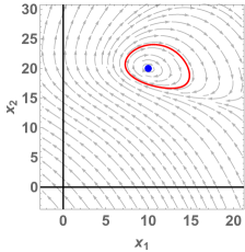
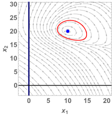
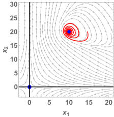
         (b)                                       (d)                                        (f)

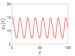
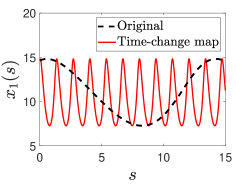
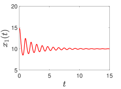
Figure 1: Application of chemical maps on dynamical system (9). Panel (a) displays the state-space for the original system $(\ref{eq:ex1_translated2})$, with the vector field shown as gray arrows, the equilibrium as the blue dot, and the limit cycle as the red curve; panel (b) displays the corresponding $(t,x_{1})$-space. Panels (c) and (d) show analogous plots system $(\ref{eq:ex1_timechange})$, which is obtained by applying the time-change map on $(\ref{eq:ex1_translated2})$. Analogous plots are shown in panels (e) and (f) for system $(\ref{eq:xfactorable})$, which is obtained by applying the $\mathbf{x}$-factorable map on $(\ref{eq:ex1_translated2})$.

From this consideration, it follows that the time-change map is a chemical one. In particular, this map qualitatively preserves every trajectory that remains within the positive quadrant. We verify this fact in Figure 1(c), which shows the state-space for (12). However, the time change-map displays three undesirable features. Firstly, it introduces a continuum of equilibria on the $x_{2}$-axis, which we show in blue in Figure 1(c). Consequently, for initial conditions in certain regions, the solutions of (12) approach the $x_{2}$-axis - a behavior qualitatively different from the original system (9). This property arises from the fact that (13) is not differentiable at time $t$ such that $x_{1}(t)=0$. Secondly, period of oscillations is significantly changed under this map. In particular, since $x_{1}(t)$ oscillates around the equilibrium $x_{1}^{*}=10$, it follows from (13) that the period is reduced roughly by a factor of $10$. This observation is confirmed in Figure 1(d): we show in red the limit cycle of (12) in the $(s,x_{1})$-space, together with the limit cycle of (9) as the black dashed curve. Finally, the time-change map in general significantly increases the degree of polynomial systems, i.e. degree $m$ can be significantly larger than $n$ in Definition 3.1. For example, if (9) also had a non-chemical term in the second equation, then the vector fields would have to be multiplied by $x_{1}x_{2}$. See Appendix B and e.g. [11, 12] for more details about the time-change map.

3.2 $\mathbf{x}$-factorable map

Let us now multiply the vector field in the first equation of (9) by $x_{1}$, and that in the second equation by $x_{2}$, thus obtaining

$$\frac{\mathrm{d}x_{1}}{\mathrm{d}t} =x_{1}\left(-\frac{45}{4}+\frac{1}{8}x_{1}+\frac{1}{2}x_{2}\right),$$

$$\frac{\mathrm{d}x_{2}}{\mathrm{d}t} =x_{2}\left(\frac{135}{8}+\frac{1}{2}x_{1}-\frac{51}{32}x_{2}-\frac{1}{20}x_{1}x_{2}+\frac{1}{20}x_{2}^{2}\right).$$ (14)

The map that transforms the dynamical system (9) into the chemical system (14) is called an $\mathbf{x}$-factorable map [14]. More generally, the $\mathbf{x}$-factorable map can be applied systematically as follows: multiply the vector field $g_{i}$ in equation $i$ from (4) by $x_{i}$ for all $i=1,2,\ldots,N$. The state-space for (14) is shown in Figure 1(e), while the corresponding $(t,x_{1})$-space in Figure 1(f). Note that (14) has some equilibria on the boundary of $\mathbb{R}_{\geq}$; one of them, namely $(0,0)$, is shown as a blue dot in Figure 1(e). One can notice that the $\mathbf{x}$-factorable map has reversed stability of the target equilibrium and destroyed the limit cycle.

In contrast to the failure of the $\mathbf{x}$-factorable map in Figure 1(e)–(f), a number of examples are presented in [14] showing that this map can in some sense preserve equilibria, limit cycles, and even chaotic attractors; however, no rigorous results are put forward. Instead, the authors from [14] suggest a heuristic: to preserve a dynamical feature of interest, it should be translated sufficiently far from the axes in the state-space before the map is applied. Let us now prove by counter-example that this heuristic can fail even for hyperbolic equilibria.

Counter-example. Consider a perturbed harmonic oscillator

$$\frac{\mathrm{d}y_{1}}{\mathrm{d}t} =\frac{1}{2}y_{2}+\frac{25}{2}\varepsilon^{2}y_{1},$$

$$\frac{\mathrm{d}y_{2}}{\mathrm{d}t} =-\frac{1}{2}y_{1}+\frac{1}{2}\varepsilon\left(-y_{1}y_{2}+y_{2}^{2}\right)-\frac{75}{8}\varepsilon^{2}y_{2}.$$ (15)

Using e.g. theory from [1][Chapter 4.11], one can show that (15) has an unstable robust spiral at the origin surrounded by a unique stable hyperbolic limit cycle for all $\varepsilon>0$ sufficiently small. Under the translational change of variables $x_{1}=(y_{1}+10)$, $x_{2}=(y_{2}+20)$ and with $\varepsilon=1/10$, system (15) becomes (9).

Let us now fix $\varepsilon=1/10$, translate the variables via $x_{1}=(y_{1}+1/\mu)$ and $x_{2}=(y_{2}+2/\mu)$ in (15), where $\mu>0$ is a parameter, and then apply the $\mathbf{x}$-factorable map, thus obtaining system

$$\frac{\mathrm{d}x_{1}}{\mathrm{d}t} =x_{1}\left[\frac{1}{2}\left(x_{2}-\frac{2}{\mu}\right)+\frac{1}{8}\left(x_{1}-\frac{1}{\mu}\right)\right],$$

$$\frac{\mathrm{d}x_{2}}{\mathrm{d}t} =x_{2}\left[-\frac{1}{2}\left(x_{1}-\frac{1}{\mu}\right)-\frac{1}{20}\left(x_{1}-\frac{1}{\mu}\right)\left(x_{2}-\frac{2}{\mu}\right)+\frac{1}{20}\left(x_{2}-\frac{2}{\mu}\right)^{2}-\frac{3}{32}\left(x_{2}-\frac{2}{\mu}\right)\right],$$ (16)

which reduces to (14) if $\mu=1/10$. Does the heuristic from [14] hold, i.e. does the equilibrium $(1/\mu,2/\mu)$ from (16) qualitatively match the unstable spiral $(10,20)$ from (9) if $\mu>0$ is sufficiently small? One can readily show that $(1/\mu,2/\mu)$ is a stable spiral for all $\mu>0$, i.e. no matter how far it is translated from the boundary of $\mathbb{R}_{\geq}^{2}$. Therefore, the heuristic fails, and the $\mathbf{x}$-factorable map, not even preserving the hyperbolic equilibrium, is not chemical.

4 Quasi-chemical map

In this section, we introduce a novel chemical map, beginning with the following two examples.

Example. Let us fix $\varepsilon=1/10$ in system (15), and perturb its vector field as follows

$$\frac{\mathrm{d}z_{1}}{\mathrm{d}t} =\frac{1}{2}z_{2}+\frac{1}{8}z_{1}+\mu z_{1}\left[\frac{1}{2}z_{2}+\frac{1}{8}z_{1}\right],$$

$$\frac{\mathrm{d}z_{2}}{\mathrm{d}t} =-\frac{1}{2}z_{1}+\frac{1}{20}\left(-z_{1}z_{2}+z_{2}^{2}\right)-\frac{3}{32}z_{2}+\frac{\mu}{2}z_{2}\left[-\frac{1}{2}z_{1}+\frac{1}{20}\left(-z_{1}z_{2}+z_{2}^{2}\right)-\frac{3}{32}z_{2}\right].$$ (17)

In particular, we have perturbed the first component of the vector field by itself multiplied by $z_{1}$, and similarly for the second component. Due to robustness (see Definition 2.1), there exists $\mu_{0}>0$ such that for all $\mu\in(0,\mu_{0})$ system (17) displays an equilibrium surrounded by a limit cycle which are arbitrarily close and qualitatively equivalent to those of (15). We now exploit these perturbations to make (17) chemical. To this end, let us fix $\mu\in(0,\mu_{0})$ and translate the variables via $x_{1}=(z_{1}+1/\mu)$ and $x_{2}=(z_{2}+2/\mu)$, leading to the qualitatively equivalent chemical system

$$\frac{\mathrm{d}x_{1}}{\mathrm{d}t} =\mu x_{1}\left[\frac{1}{2}\left(x_{2}-\frac{2}{\mu}\right)+\frac{1}{8}\left(x_{1}-\frac{1}{\mu}\right)\right],$$

$$\frac{\mathrm{d}x_{2}}{\mathrm{d}t} =\frac{\mu}{2}x_{2}\left[-\frac{1}{2}\left(x_{1}-\frac{1}{\mu}\right)-\frac{1}{20}\left(x_{1}-\frac{1}{\mu}\right)\left(x_{2}-\frac{2}{\mu}\right)+\frac{1}{20}\left(x_{2}-\frac{2}{\mu}\right)^{2}-\frac{3}{32}\left(x_{2}-\frac{2}{\mu}\right)\right].$$ (18)

Fixing $\mu=1/10$ in (18), one obtains

$$\frac{\mathrm{d}x_{1}}{\mathrm{d}t} =\frac{x_{1}}{10}\left(-\frac{45}{4}+\frac{1}{8}x_{1}+\frac{1}{2}x_{2}\right),$$

$$\frac{\mathrm{d}x_{2}}{\mathrm{d}t} =\frac{x_{2}}{20}\left(\frac{135}{8}+\frac{1}{2}x_{1}-\frac{51}{32}x_{2}-\frac{1}{20}x_{1}x_{2}+\frac{1}{20}x_{2}^{2}\right).$$ (19)

In Figure 2(a), we display the state-space for (19) which contains an unstable equilibrium (blue dot) enclosed by a stable limit cycle (red curve), in qualitative agreement with (15) (and, therefore (9)). Note that (19) can be obtained from the $\mathbf{x}$-factorable system (14) by a suitable rescaling of the vector field; let us stress, however, that (14) itself does not qualitatively match with the target system, see Figure 1(e)–(f).

In Figure 2(a), we also show the limit cycle of (9) as dashed black curve, which is in quantitative disagreement with the limit cycle of (19). By design, this mismatch can be made arbitrarily small if $\mu$ is chosen sufficiently small. For example, in Figure 2(b), we display the state-space for (18) with $\mu=1/100$, where one can notice a significantly improved match with the target limit cycle. A corresponding time-state space is shown in Figure 2(c), demonstrating that the period of oscillations is also approximately preserved.

      (a) (18) with $\mu=1/10$           (b) (18) with $\mu=1/100$           (c) (18) with $\mu=1/100$

       

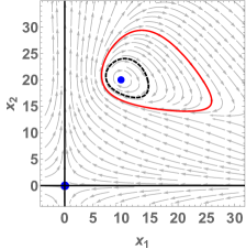
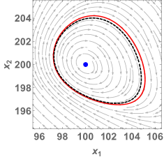
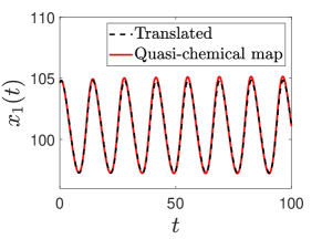
      (d) (21) with $\mu=1/10$           (e) (21) with $\mu=1/100$           (f) (21) with $\mu=1/100$

       

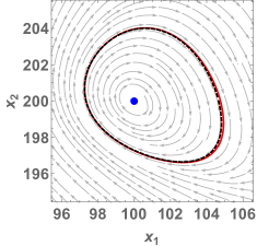
Figure 2: Application of the quasi-chemical map (24) on dynamical system (15). Panel (a) displays state-space for system $(\ref{eq:ex1_P1c})$ with $\mu=1/10$, with the limit cycle shown as the red curve, the equilibrium as the blue dot, and vector field as gray arrows; also shown is the limit cycle of $(\ref{eq:ex1_translated2})$ as the black dashed curve. Panel (b) displays a similar plot for $(\ref{eq:ex1_P1c})$ with $\mu=1/100$, while panel $(c)$ shows the corresponding time-state space. Analogous plots are shown in panels (d)–(f) for system $(\ref{eq:ex1_P2c})$.

Example. Consider again system (15) with $\varepsilon=1/10$, and let us now perturb only the first equation, leading to

$$\frac{\mathrm{d}z_{1}}{\mathrm{d}t} =\frac{1}{2}z_{2}+\frac{1}{8}z_{1}+\mu z_{1}\left[\frac{1}{2}z_{2}+\frac{1}{8}z_{1}\right],$$

$$\frac{\mathrm{d}z_{2}}{\mathrm{d}t} =-\frac{1}{2}z_{1}+\frac{1}{20}\left(-z_{1}z_{2}+z_{2}^{2}\right)-\frac{3}{32}z_{2}.$$ (20)

Translating the variables according to $x_{1}=(z_{1}+1/\mu)$ and $x_{2}=(z_{2}+2/\mu)$, one obtains the qualitatively equivalent system

$$\frac{\mathrm{d}x_{1}}{\mathrm{d}t} =\mu x_{1}\left[\frac{1}{2}\left(x_{2}-\frac{2}{\mu}\right)+\frac{1}{8}\left(x_{1}-\frac{1}{\mu}\right)\right],$$

$$\frac{\mathrm{d}x_{2}}{\mathrm{d}t} =-\frac{1}{2}\left(x_{1}-\frac{1}{\mu}\right)-\frac{1}{20}\left(x_{1}-\frac{1}{\mu}\right)\left(x_{2}-\frac{2}{\mu}\right)+\frac{1}{20}\left(x_{2}-\frac{2}{\mu}\right)^{2}-\frac{3}{32}\left(x_{2}-\frac{2}{\mu}\right).$$ (21)

One can readily show that the vector field in the second equation is chemical for all sufficiently small $\mu$, making (21) chemical then. Fixing $\mu=1/10$ in (21), one gets

$$\frac{\mathrm{d}x_{1}}{\mathrm{d}t} =\frac{x_{1}}{10}\left(-\frac{45}{4}+\frac{1}{8}x_{1}+\frac{1}{2}x_{2}\right),$$

$$\frac{\mathrm{d}x_{2}}{\mathrm{d}t} =\frac{135}{8}+\frac{1}{2}x_{1}-\frac{51}{32}x_{2}-\frac{1}{20}x_{1}x_{2}+\frac{1}{20}x_{2}^{2}.$$ (22)

In Figure 2(d), we display the state-space of (22), showing an unstable equilibrium and a stable limit cycle which are in qualitative agreement with (9). Figure 2(e)–(f) displays the state and time-state spaces for (21) when $\mu=1/100$, showing an excellent quantitative match with the target system. Let us stress that, as opposed to (18) which is cubic, system (21) is quadratic.

Quasi-chemical map. Let us now define the map underlying (18) and (21). This map consists of two steps: firstly, the vector field is perturbed and, secondly, the variables are then suitably translated. In particular, let us perturb system (1) as follows:

$$\frac{\mathrm{d}z_{i}}{\mathrm{d}t} =f_{i}(\mathbf{z})+\mu\frac{z_{i}}{T_{i}}\left[f_{i}(\mathbf{z})-q_{i}(\mathbf{z})\right],\;\;\;i=1,2,\ldots,N,$$ (23)

where $\mu>0$ is a free parameter, $T_{i}>0$ a fixed parameter, and $q_{i}(\mathbf{x})\in\mathbb{P}_{n}(\mathbb{R}^{N},\mathbb{R})$ an arbitrary polynomial of degree at most $n$ for all $i=1,2,\ldots,N$; in what follows, we also let $\mathbf{T}=(T_{1},T_{2},\ldots,T_{N})^{\top}\in\mathbb{R}_{>}^{N}$. For all sufficiently small $\mu>0$, (23) preserves robust features of (1). To make (23) chemical, we translate the variables via $x_{i}=(z_{i}+T_{i}/\mu)$, which leads to system (24), and motivates the following definition.

Definition 4.1.

$($Quasi-chemical map$)$ Consider system $(\ref{eq:dyn_components})$. Consider also system

$$\frac{\mathrm{d}x_{i}}{\mathrm{d}t} =q_{i}\left(\mathbf{x}-\frac{\mathbf{T}}{\mu}\right)+\frac{\mu}{T_{i}}x_{i}\Big{[}f_{i}\left(\mathbf{x}-\frac{\mathbf{T}}{\mu}\right)-q_{i}\left(\mathbf{x}-\frac{\mathbf{T}}{\mu}\right)\Big{]},\;\;\;i=1,2,\ldots,N,$$ (24)

where $q_{i}(\mathbf{x}-\mathbf{T}/\mu)\in\mathbb{P}_{n}^{\mathcal{C}}(\mathbb{R}^{N},\mathbb{R})$ are arbitrary polynomials of degree at most $n$ that are chemical for all sufficiently small $\mu>0$ and for all $i=1,2,\ldots,N$; we say that $q_{i}(\mathbf{x})$ are quasi-chemical. Then, $\Psi_{\mu}:\mathbb{P}_{n}(\mathbb{R}^{N},\mathbb{R}^{N})\to\mathbb{P}_{n+1}^{\mathcal{C}}(\mathbb{R}^{N},\mathbb{R}^{N})$, mapping the dynamical system $(\ref{eq:dyn_components})$ to the chemical system $(\ref{eq:quasi_chemical})$ for all sufficiently small $\mu>0$, is called a quasi-chemical map.

Definitions 2.1 and 3.1, together with equation (23), imply that the quasi-chemical map is a chemical one when it comes to preserving robust regions in the state-space. To state this more precisely, for any given set $\mathbb{U}\subset\mathbb{R}^{N}$ and vector $\mathbf{T}\in\mathbb{R}^{N}$, we let $\mathbb{U}+\mathbf{T}=\{\mathbf{x}+\mathbf{T}\in\mathbb{R}^{N}\,|\,\mathbf{x}\in\mathbb{U}\}$.

Theorem 4.1.

$($Quasi-chemical map$)$ Consider a dynamical system $(\ref{eq:dyn_components})$ which is robust in a state-space region $\mathbb{U}\subset\mathbb{R}^{N}$. Then, for all sufficiently small $\mu>0$ chemical system $(\ref{eq:quasi_chemical})$ in $\mathbb{U}+\mathbf{T}/\mu\subset\mathbb{R}_{\geq}^{N}$ is qualitatively equivalent to the dynamical system $(\ref{eq:dyn_components})$ in $\mathbb{U}$.

Remark. Theorem 4.1 holds, not only for the class of polynomial dynamical systems that are robust (i.e. remain qualitatively equivalent under any polynomial perturbation) in $\mathbb{U}\subset\mathbb{R}^{N}$, but more broadly for any dynamical system (1) that remains qualitatively equivalent in $\mathbb{U}\subset\mathbb{R}^{N}$ under the special $(n+1)$-degree perturbations from (23), which we call chemical perturbations.

Remark. Theorem 4.1 guarantees that the quasi-chemical map qualitatively preserves robust dynamical features. At the quantitative level, one may expect that the features are only slightly perturbed. In Theorem C.1 in Appendix C, we confirm that this is indeed the case for e.g. trajectories over finite time-intervals, hyperbolic equilibria and limit cycles, and trapping regions - these features remain arbitrarily close to those of suitably translated target system. Furthermore, eigenvalues, characteristic exponents and periods of oscillations also remain arbitrarily close to those of the target system. One consequence of these facts is that the quasi-chemical map preserves, not only stability, but also the type of hyperbolic equilibria.

Let us now explicitly state a special case of Theorem 4.1.

Theorem 4.2.

Consider $N$-dimensional $n$-degree dynamical system $(\ref{eq:dyn_components})$ which is robust in region $\mathbb{U}\subset\mathbb{R}^{N}$. Then, for all sufficiently small $\mu>0$ the $N$-dimensional $(n+1)$-degree chemical system

$$\frac{\mathrm{d}x_{i}}{\mathrm{d}t} =\frac{\mu}{T_{i}}x_{i}f_{i}\left(\mathbf{x}-\frac{\mathbf{T}}{\mu}\right),\;\;\;i=1,2,\ldots,N,$$ (25)

in $\mathbb{U}+\mathbf{T}/\mu\subset\mathbb{R}_{\geq}^{N}$ is qualitatively equivalent to $(\ref{eq:dyn_components})$ in $\mathbb{U}$.

Proof.

Fixing the quasi-chemical function $q_{i}=0$ for $i=1,2,\ldots,N$ in (24), one obtains (25). ∎

Theorem 4.2 shows that, given any polynomial dynamical system, one can always translate its variables by $T_{i}/\mu$ and multiply its $i$th right-hand side by $(\mu/T_{i})x_{i}$ to obtain for sufficiently small $\mu>0$ a chemical system which has qualitatively equivalent robust dynamical features. If one is prepared to increase the polynomial degree by one when mapping a dynamical into chemical system, then the quasi-chemical map of the form (25) suffices. In particular, all of the dynamical systems considered in the following sections can be immediately mapped to chemical ones using (25). More broadly, one can utilize the quasi-chemical map (24) and choose functions $q_{i}$ to reduce the number of higher-degree terms in the resulting chemical systems, or even preserve the degree of the target dynamical systems, as exemplified by (21).

Before closing this section, let us note that we also present a more general form of the quasi-chemical map in Appendix C.1. In this context, we allow general perturbations of the vector field, and we allow both scaling and translation to be applied to the dependent variables, with different variables in general scaled differently. This generalized map can be e.g. used to magnify dynamical features as they are translated further and further from the state-space boundary, see the example in Appendix C.1 and Figure 7. The generalized quasi-chemical map is also used to design a quadratic chemical system undergoing a global bifurcation, see Appendix D.

5 Chemical system with arbitrary many limit cycles

Let us consider the two-dimensional dynamical system

$$\frac{\mathrm{d}y_{1}}{\mathrm{d}t} =y_{2}+\varepsilon(\beta_{0}y_{1}+\beta_{1}y_{1}^{3}+\ldots+\beta_{n}y_{1}^{2n+1}),$$

$$\frac{\mathrm{d}y_{2}}{\mathrm{d}t} =-y_{1}.$$ (26)

Under suitable choice of the coefficients $\beta_{0},\beta_{1},\ldots,\beta_{n}$, and for all $\varepsilon>0$ sufficiently small, (26) has $\lfloor(n-1)/2\rfloor$ hyperbolic limit cycles [17, 1], where $\lfloor\cdot\rfloor$ denotes the integer part of a positive real number. We also prove this fact, and provide explicit expressions for a suitable set of coefficients, in Appendix E. We now map (26) into a chemical system of the same degree. To this end, we denote two irreversible reactions $nX\xrightarrow[]{\alpha}mX$ and $mX\xrightarrow[]{\beta}nX$ as a single reversible reaction $nX\xrightleftharpoons[\beta]{\alpha}mX$.

Theorem 5.1.

$($Chemical system with arbitrary many limit cycles$)$ Consider the CRN

$$\varnothing \xrightleftharpoons[\alpha_{1}]{\alpha_{0}}X_{1},\;\;2X_{1}\xrightleftharpoons[\alpha_{3}]{\alpha_{2}}3X_{1},\;\;\ldots,\;\;2nX_{1}\xrightleftharpoons[\alpha_{2n+1}]{\alpha_{2n}}(2n+1)X_{1},$$

$$X_{2} \xrightarrow[]{\alpha_{2n+2}}X_{1}+2X_{2},\;\;X_{1}+X_{2}\xrightarrow[]{\alpha_{2n+3}}X_{1}.$$ (27)

Let $0<r_{1}<r_{2}<\ldots<r_{n}$ be arbitrary real numbers. Then, there exist coefficients $\alpha_{i}=\alpha_{i}(r_{1},r_{2},\ldots,r_{N})$ for $i=0,1,\ldots,2N+3$ such that CRN $(\ref{eq:HO_1_C})$ has $n$ hyperbolic limit cycles. The $i$th limit cycle is arbitrarily close to $x_{1}(t)=r_{i}\cos(t)$ and $x_{2}(t)=-r_{i}\sin(t)$, and has period arbitrarily close to $2\pi$. The $n$th limit cycle is stable, and the limit cycles alternate in stability.

Proof.

Let us fix $\varepsilon>0$ to a sufficiently small value, and let us also fix $\beta_{0},\beta_{1},\ldots,\beta_{n}$ according to (69) from Appendix E; in particular, we choose $\beta_{n}<0$. Consider the perturbed system

$$\frac{\mathrm{d}z_{1}}{\mathrm{d}t} =z_{2}+\varepsilon(\beta_{0}z_{1}+\beta_{1}z_{1}^{3}+\ldots+\beta_{n}z_{1}^{2n+1}),$$

$$\frac{\mathrm{d}z_{2}}{\mathrm{d}t} =-z_{1}-\mu z_{1}z_{2},$$

which is of the form (23) with $q_{1}=f_{1}$ and $q_{2}=0$. Under translation $x_{1}=(z_{1}+1/\mu)$ and $x_{2}=(z_{2}+1/\mu)$, one obtains:

$$\frac{\mathrm{d}x_{1}}{\mathrm{d}t} =\left(x_{2}-\frac{1}{\mu}\right)+\varepsilon\sum_{i=0}^{n}\beta_{i}\left(x_{1}-\frac{1}{\mu}\right)^{2i+1}=\sum_{i=0}^{2n+1}(-1)^{i}\alpha_{i}x_{1}^{i}+\alpha_{2n+2}x_{2},$$

$$\frac{\mathrm{d}x_{2}}{\mathrm{d}t} =-\mu x_{2}\left(x_{1}-\frac{1}{\mu}\right)=\alpha_{2n+2}x_{2}-\alpha_{2n+3}x_{1}x_{2},$$ (28)

with the coefficients $\alpha_{0},\alpha_{1},\ldots,\alpha_{2n+3}$ given by (70) in Appendix E. Since $\beta_{n}<0$, the zero-degree term in the first equation from (28) is dominated by $1/\mu^{2n+1}>0$ for all sufficiently small $\mu>0$; therefore, system (28) is then chemical. The CRN induced by (28) is given by (27); see Definition 2.3. More specifically, the canonical reactions $X_{2}\xrightarrow[]{1}X_{1}+X_{2}$ and $X_{2}\xrightarrow[]{1}2X_{2}$ can be fused into $X_{2}\xrightarrow[]{1}X_{1}+2X_{2}$; see Definition 2.4. Statement of the theorem follows from Theorem 4.1 specialized to limit cycles; in particular, see Theorem C.1(iii) from Appendix C. ∎

                      (a)                                                         (b)

             

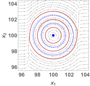
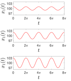
Figure 3: Chemical system with arbitrary many limit cycles. Panel (a) displays state-space for chemical system $(\ref{eq:HO_1_RREn5})$, corresponding to the CRN $(\ref{eq:HO_1_Cn5})$, with parameters $(\ref{eq:HO_1_RREn5coeff})$, $\varepsilon=10^{-4}$ and $\mu=10^{-2}$. The three stable and two unstable limit cycles are respectively shown as solid red and dashed blue curves, and the enclosed equilibrium as the blue dot. Each of the three stable limit cycles is shown in the time-state space in one of the sub-panels of panel (b).

Example. Consider the CRN (27) with $n=5$:

$$\varnothing \xrightleftharpoons[\alpha_{1}]{\alpha_{0}}X_{1},\;\;2X_{1}\xrightleftharpoons[\alpha_{3}]{\alpha_{2}}3X_{1},\;\;4X_{1}\xrightleftharpoons[\alpha_{5}]{\alpha_{4}}5X_{1},\;\;6X_{1}\xrightleftharpoons[\alpha_{7}]{\alpha_{6}}7X_{1},\;\;8X_{1}\xrightleftharpoons[\alpha_{9}]{\alpha_{8}}9X_{1},\;\;10X_{1}\xrightleftharpoons[\alpha_{11}]{\alpha_{10}}11X_{1},$$

$$X_{2} \xrightarrow[]{\alpha_{12}}X_{1}+2X_{2},\;\;X_{1}+X_{2}\xrightarrow[]{\alpha_{13}}X_{1},$$ (29)

with the chemical system written for simplicity in the form

$$\frac{\mathrm{d}x_{1}}{\mathrm{d}t} =\left(x_{2}-\frac{1}{\mu}\right)+\varepsilon\sum_{i=0}^{5}\beta_{i}\left(x_{1}-\frac{1}{\mu}\right)^{2i+1},$$

$$\frac{\mathrm{d}x_{2}}{\mathrm{d}t} =-\mu x_{2}\left(x_{1}-\frac{1}{\mu}\right).$$ (30)

Let us impose that (30) has $5$ limit cycles, close to circles with radii $r_{1}=1$, $r_{2}=3/2$, $r_{3}=2$, $r_{4}=5/2$ and $r_{5}=3$. Then, suitable coefficients $\beta_{0},\beta_{1},\ldots,\beta_{5}$ are given

$$\beta_{0} =\frac{2025}{4},\;\;\beta_{1}=-\frac{5307}{4},\;\;\beta_{2}=1039,\;\;\beta_{3}=-\frac{11652}{35},\;\;\beta_{4}=\frac{320}{7},\;\;\beta_{5}=-\frac{512}{231}.$$ (31)

Coefficients (31) can be obtained directly from (69) in Appendix E; alternatively, one can indirectly impose that a suitable polynomial has the desired radii as roots, see (68) in Appendix E. In Figure 3(a), we display the state-space for chemical system (30) with parameters (31), $\varepsilon=10^{-4}$ and $\mu=10^{-2}$. As desired, the system has three stable limit cycles, shown as red solid curves, and two unstable ones, shown as dashed blue curves, all of which are approximately circular. In Figure 3(b), we show three sub-panels, each displaying one of the stable limit cycles in the time-state space; one can notice that each of the limit cycles is approximately $2\pi$-periodic.

6 Chemical systems with chaos

In this section, we design some chemical systems whose long-time dynamics is neither an equilibrium nor a limit cycle. To this end, let us consider the Lorenz system [18]:

$$\frac{\mathrm{d}y_{1}}{\mathrm{d}t} =-10y_{1}+10y_{2},$$

$$\frac{\mathrm{d}y_{2}}{\mathrm{d}t} =28y_{1}-y_{2}-y_{1}y_{3},$$

$$\frac{\mathrm{d}y_{3}}{\mathrm{d}t} =-\frac{8}{3}y_{3}+y_{1}y_{2}.$$ (32)

In Figure 4(a), we show the butterfly-like chaotic attractor of (32), called the Lorenz attractor, projected into the $(y_{1},y_{3})$-space, while the corresponding $(t,y_{1})$-space is shown in Figure 4(b).

                   (a)                                                            (c)

             

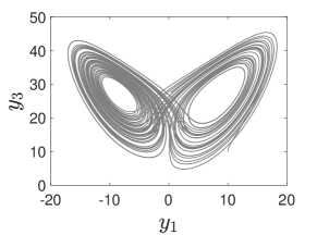
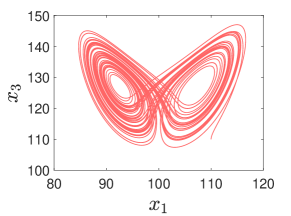
                   (b)                                                            (d)

             

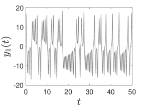
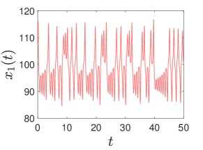
Figure 4: Chemical system with Lorenz attractor. Panels (a)–(b) display the $(y_{1},y_{3})$-space and the $(t,y_{1})$-space for the Lorenz system $(\ref{eq:Lorenz})$ with the initial condition $y_{1}(0)=y_{2}(0)=y_{3}(0)=10$. Analogous plots are shown in panels (c)–(d) for the chemical system $(\ref{eq:Lorenz_chemical})$ with the initial condition $x_{1}(0)=x_{2}(0)=x_{3}(0)=10+100$.

Theorem 6.1.

$($Chemical system with Lorenz attractor$)$ Consider the CRN

$$X_{1} \xrightarrow[]{\alpha_{1}}\varnothing,\;\;\;X_{2}\xrightarrow[]{\alpha_{2}}X_{1}+X_{2},\;\;\;\varnothing\xrightleftharpoons[\alpha_{4}]{\alpha_{3}}X_{2},\;\;\;X_{1}+X_{2}\xrightarrow[]{\alpha_{5}}X_{1}+2X_{2},\;\;\;X_{2}+X_{3}\xrightarrow[]{\alpha_{6}}2X_{2},$$

$$X_{1} +X_{2}+X_{3}\xrightarrow[]{\alpha_{7}}X_{1}+2X_{3},\;\;\;\varnothing\xrightarrow[]{\alpha_{8}}X_{3},\;\;\;X_{3}\xrightarrow[]{\alpha_{9}}2X_{3},\;\;\;X_{1}+X_{3}\xrightarrow[]{\alpha_{10}}X_{1}.$$ (33)

Assume that the rate coefficients are given by

$$\alpha_{1} =10,\;\;\;\alpha_{2}=10,\;\;\;\alpha_{3}=\frac{1}{\mu},\;\;\;\alpha_{4}=\frac{1}{\mu}+29,\;\;\;\alpha_{5}=1+28\mu,\;\;\;\alpha_{6}=1,$$

$$\alpha_{7} =\mu,\;\;\;\alpha_{8}=\frac{8}{3\mu},\;\;\;\alpha_{9}=\frac{1}{\mu}-\frac{8}{3},\;\;\;\alpha_{10}=1.$$ (34)

Then, for every sufficiently small $\mu>0$, CRN $(\ref{eq:Lorenz_CRN})$ has a chaotic attractor which is qualitatively equivalent to the Lorenz attractor.

Proof.

Consider the perturbed Lorenz system

$$\frac{\mathrm{d}z_{1}}{\mathrm{d}t} =-10z_{1}+10z_{2},$$

$$\frac{\mathrm{d}z_{2}}{\mathrm{d}t} =28z_{1}-z_{2}-z_{1}z_{3}+\mu z_{2}\left[28z_{1}-z_{1}z_{3}\right],$$

$$\frac{\mathrm{d}z_{3}}{\mathrm{d}t} =-\frac{8}{3}z_{3}+z_{1}z_{2}+\mu z_{1}z_{2}z_{3},$$

which is of the form (23) with $q_{1}=f_{1}$, $q_{2}=-z_{2}$, and $q_{3}=-(8/3)z_{3}$. Translating the variables via $x_{i}=(z_{i}+1/\mu)$ for all $i=1,2,3$, one obtains

$$\frac{\mathrm{d}x_{1}}{\mathrm{d}t} =-10x_{1}+10x_{2},$$

$$\frac{\mathrm{d}x_{2}}{\mathrm{d}t} =-\left(x_{2}-\frac{1}{\mu}\right)+\mu x_{2}\left[28\left(x_{1}-\frac{1}{\mu}\right)-\left(x_{1}-\frac{1}{\mu}\right)\left(x_{3}-\frac{1}{\mu}\right)\right],$$

$$\frac{\mathrm{d}x_{3}}{\mathrm{d}t} =-\frac{8}{3}\left(x_{3}-\frac{1}{\mu}\right)+\mu x_{3}\left[\left(x_{1}-\frac{1}{\mu}\right)\left(x_{2}-\frac{T}{\mu}\right)\right].$$ (35)

For all sufficiently small $\mu>0$, system (35) is chemical, and induces CRN (33) with rate coefficients (34). Statement of the theorem follows from the fact that the Lorenz attractor is robust with respect to all smooth perturbations [19]. ∎

Let us fix $\mu=1/100$ in (34); chemical system induced by (33) is then given by

$$\frac{\mathrm{d}x_{1}}{\mathrm{d}t} =-10x_{1}+10x_{2},$$

$$\frac{\mathrm{d}x_{2}}{\mathrm{d}t} =100-129x_{2}+\frac{32}{25}x_{1}x_{2}+x_{2}x_{3}-\frac{1}{100}x_{1}x_{2}x_{3},$$

$$\frac{\mathrm{d}x_{3}}{\mathrm{d}t} =\frac{800}{3}+\frac{292}{3}x_{3}-x_{1}x_{3}-x_{2}x_{3}+\frac{1}{100}x_{1}x_{2}x_{3}.$$ (36)

The state-space and time-state space for (36) are respectively shown in Figure 4(c) and (d), which compare well with Figure 4(a)–(b). Note that the Lorenz system (32) and its chemical counterpart (36) evolve on a similar time-scale. Note also that, while the Lorenz attractor itself is robust with respect to perturbations, the underlying trajectories in the time-state space are sensitive; for this reason, the two trajectories shown in Figures 4(b) and (d) are different after some time.

6.1 Quadratic system

Chemical Lorenz system (36) contains a cubic term, i.e. the induced CRN (33) contains one tri-molecular reaction. Let us now focus on deriving a quadratic chemical system with chaos. To this end, consider the dynamical system

$$\frac{\mathrm{d}y_{1}}{\mathrm{d}t} =\frac{27}{10}y_{2}+y_{3},$$

$$\frac{\mathrm{d}y_{2}}{\mathrm{d}t} =-y_{1}+y_{2}^{2},$$

$$\frac{\mathrm{d}y_{3}}{\mathrm{d}t} =y_{1}+y_{2},$$ (37)

which has been put forward as displaying a chaotic attractor in [20] as “Case P”. This attractor has been numerically investigated, see also Figure 5(a)–(b); however, no rigorous proofs are given. Note that proving existence and properties of chaotic attractors can be a difficult task. For example, there is a gap of more than three decades between numerical evidence of the Lorenz attractor [18] and its rigorous proof [19]. To proceed, in this paper we simply assume that (37) has a robust chaotic attractor, which allows us to state the following result.

                   (a)                                                            (c)

             

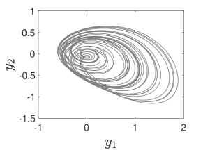
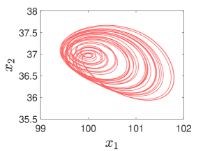
                   (b)                                                            (d)

             

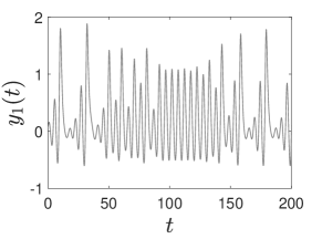
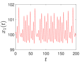
Figure 5: Quadratic chemical system with chaos. Panels (a)–(b) display the $(y_{1},y_{2})$-space and the $(t,y_{1})$-space for system $(\ref{eq:Sprott_P})$, given as [20][Case P], with the initial condition $y_{1}(0)=y_{2}(0)=y_{3}(0)=5/100$. Panels (c)–(d) show analogous plots for chemical system $(\ref{eq:Sprott_P_chemical})$ with the initial condition $x_{1}(0)=x_{3}(0)=5/100+100$ and $x_{2}(0)=5/100+1000/27$.

Theorem 6.2.

$($Quadratic chemical system with a chaotic attractor$)$ Assume that dynamical system $(\ref{eq:Sprott_P})$ has a chaotic attractor which is robust. Consider the CRN

$$X_{1} \xrightarrow[]{\alpha_{1}}\varnothing,\;\;\;X_{1}+X_{2}\xrightarrow[]{\alpha_{2}}2X_{1},\;\;\;X_{1}+X_{3}\xrightarrow[]{\alpha_{3}}2X_{1}+2X_{3},\;\;\;\varnothing\xrightleftharpoons[\alpha_{5}]{\alpha_{4}}X_{2},$$

$$2X_{2} \xrightarrow[]{\alpha_{6}}3X_{2},\;\;\;X_{3}\xrightarrow[]{\alpha_{7}}\varnothing,\;\;\;X_{2}+X_{3}\xrightarrow[]{\alpha_{8}}X_{2}+2X_{3}.$$ (38)

Assume that the rate coefficients are given by

$$\alpha_{1} =2,\;\;\;\alpha_{2}=\frac{27}{10}\mu,\;\;\;\alpha_{3}=\mu,\;\;\;\alpha_{4}=\frac{100}{729\mu^{2}},\;\;\;\alpha_{5}=\frac{20}{27\mu}-\frac{27}{10},\;\;\;\alpha_{6}=1,\;\;\;\alpha_{7}=\frac{37}{27},\;\;\;\alpha_{8}=\mu.$$ (39)

Then, for every sufficiently small $\mu>0$, CRN $(\ref{eq:quadratic_chaos_CRN})$ has a chaotic attractor which is qualitatively equivalent to the chaotic attractor of $(\ref{eq:Sprott_P})$.

Proof.

Consider the perturbed system

$$\frac{\mathrm{d}z_{1}}{\mathrm{d}t} =\frac{27}{10}z_{2}+z_{3}+\mu z_{1}\left[\frac{27}{10}z_{2}+z_{3}\right],$$

$$\frac{\mathrm{d}z_{2}}{\mathrm{d}t} =-z_{1}+z_{2}^{2}-\frac{27}{10}\mu z_{1}z_{2},$$

$$\frac{\mathrm{d}z_{3}}{\mathrm{d}t} =z_{1}+z_{2}+\mu z_{3}\left[z_{1}+z_{2}\right],$$ (40)

which is of the form (23) with $q_{1}=q_{3}=0$ and $q_{2}=z_{2}^{2}$, and which preserves the robust chaotic attractor of (37) for all sufficiently small $\mu>0$. Under translation $x_{1}=(z_{1}+1/\mu)$, $x_{2}=(z_{2}+10/(27\mu))$ and $x_{3}=(z_{3}+1/\mu)$, one obtains

$$\frac{\mathrm{d}x_{1}}{\mathrm{d}t} =\mu x_{1}\left[\frac{27}{10}\left(x_{2}-\frac{10}{27\mu}\right)+\left(x_{3}-\frac{1}{\mu}\right)\right],$$

$$\frac{\mathrm{d}x_{2}}{\mathrm{d}t} =\left(x_{2}-\frac{10}{27\mu}\right)^{2}+\frac{27}{10}\mu x_{2}\left[-\left(x_{1}-\frac{1}{\mu}\right)\right],$$

$$\frac{\mathrm{d}x_{3}}{\mathrm{d}t} =\mu x_{3}\left[\left(x_{1}-\frac{1}{\mu}\right)+\left(x_{2}-\frac{10}{27\mu}\right)\right].$$ (41)

The choice of the translation parameters has been made so that the monomial $x_{1}x_{2}$ appears with the same coefficient in the first two equations in (41), allowing for fusing of the underlying canonical reactions, see Definition 2.4. The induced CRN is given by (38), with rate coefficients (39). ∎

Remark. The assumption in Theorem 6.2 can be weakened: it is sufficient to assume that $(\ref{eq:Sprott_P})$ has a chaotic attractor which is robust with respect to only the chemical perturbation from (40).

Let us fix $\mu=1/100$ in (39), under which the chemical system (41) becomes

$$\frac{\mathrm{d}x_{1}}{\mathrm{d}t} =-2x_{1}+\frac{27}{1000}x_{1}x_{2}+\frac{1}{100}x_{1}x_{3},$$

$$\frac{\mathrm{d}x_{2}}{\mathrm{d}t} =\frac{10^{6}}{729}-\frac{19271}{270}x_{2}-\frac{27}{1000}x_{1}x_{2}+x_{2}^{2},$$

$$\frac{\mathrm{d}x_{3}}{\mathrm{d}t} =-\frac{37}{27}x_{3}+\frac{1}{100}x_{1}x_{3}+\frac{1}{100}x_{2}x_{3}.$$ (42)

Dynamics of (42) is shown in Figure 5(c)–(d), which compares well with the original system (37).

7 Chemical systems undergoing bifurcations

So far in this paper, we have focused on dynamical systems with fixed coefficients and in the state-space regions in which they are robust to perturbations. In such cases, Theorem 4.1 guarantees that the quasi-chemical map preserves the dynamics. In this section, we discuss systems with variable coefficients and in state-space regions in which they may be fragile to perturbations. More precisely, let us consider again dynamical system (2), and let us now explicitly indicate its dependence on parameters $\boldsymbol{\beta}\in\mathbb{R}^{P}$:

$$\frac{\mathrm{d}\mathbf{y}}{\mathrm{d}t} =\mathbf{f}(\mathbf{y};\boldsymbol{\beta}).$$ (43)

Consider also its regular perturbation (3), now denoted by

$$\frac{\mathrm{d}\mathbf{z}}{\mathrm{d}t} =\mathbf{f}(\mathbf{z};\boldsymbol{\beta})+\mathbf{p}(\mathbf{z};\mu).$$ (44)

Let us fix the parameters to $\boldsymbol{\beta}=\boldsymbol{\beta}^{*}$, and assume that then (43) is not robust in some region $\mathbb{U}\subset\mathbb{R}^{N}$. This means that, for some perturbations, systems (44) and (43) at $\boldsymbol{\beta}=\boldsymbol{\beta}^{*}$ are qualitatively different in $\mathbb{U}$, and (43) is said to be undergoing a bifurcation [1, 15]. Even though (44) at $\boldsymbol{\beta}=\boldsymbol{\beta}^{*}$ is in general qualitatively different from (43) at $\boldsymbol{\beta}=\boldsymbol{\beta}^{*}$, (44) at a slightly different parameter value, say $\boldsymbol{\beta}=\boldsymbol{\beta}(\mu)$, may be qualitatively equivalent to (43) at $\boldsymbol{\beta}=\boldsymbol{\beta}^{*}$.

Definition 7.1.

$($Robust bifurcation$)$ Assume that system $(\ref{eq:dynp})$ at $\boldsymbol{\beta}=\boldsymbol{\beta}^{*}\in\mathbb{R}^{P}$ is not robust in $\mathbb{U}\subset\mathbb{R}^{N}$, and undergoes there a bifurcation $\mathcal{B}$. Assume also that for every polynomial $\mathbf{p}(\mathbf{z};\mu)$ and for every sufficiently small $\mu>0$ there exists $\boldsymbol{\beta}(\mu)$, arbitrarily close to $\boldsymbol{\beta}^{*}$, such that regularly perturbed system $(\ref{eq:dyn3p})$ at $\boldsymbol{\beta}=\boldsymbol{\beta}(\mu)$ and system $(\ref{eq:dynp})$ at $\boldsymbol{\beta}=\boldsymbol{\beta}^{*}$ are qualitatively equivalent in $\mathbb{U}$. Then, system $(\ref{eq:dynp})$ is said to undergo at $\boldsymbol{\beta}=\boldsymbol{\beta}^{*}$ a robust bifurcation $\mathcal{B}$ in $\mathbb{U}$.

Definition 4.1 and equation (23) imply the following theorem.

Theorem 7.1.

$($Quasi-chemical map: Bifurcations$)$ Assume that system $(\ref{eq:dynp})$ at $\boldsymbol{\beta}=\boldsymbol{\beta}^{*}\in\mathbb{R}^{P}$ is not robust in $\mathbb{U}\subset\mathbb{R}^{N}$, and undergoes there a robust bifurcation $\mathcal{B}$. Then, for all sufficiently small $\mu>0$ there exists parameter value $\boldsymbol{\beta}(\mu)$, arbitrarily close to $\boldsymbol{\beta}^{*}$, such that chemical system $(\ref{eq:quasi_chemical})$ at $\boldsymbol{\beta}=\boldsymbol{\beta}(\mu)$ undergoes the bifurcation $\mathcal{B}$ in $\mathbb{U}+\mathbf{T}/\mu\subset\mathbb{R}_{\geq}^{N}$.

7.1 Homoclinic bifurcation

Consider the dynamical system

$$\frac{\mathrm{d}y_{1}}{\mathrm{d}t} =\left(\beta-\frac{4}{5}\right)y_{1}+y_{2}-\frac{6}{5}y_{1}y_{2}+\frac{3}{2}y_{2}^{2},$$

$$\frac{\mathrm{d}y_{2}}{\mathrm{d}t} =y_{1}-\frac{4}{5}y_{2}-\frac{4}{5}y_{2}^{2}.$$ (45)

At $\beta=0$, (45) undergoes a super-critical homoclinic bifurcation [21, 6]. In particular, when $\beta=0$, system (45) has a saddle equilibrium at the origin, whose stable and unstable manifolds connect, forming a tear-shaped homoclinic loop; see Figure 6(b), where we also display an unstable focus inside the homoclinic loop, and a stable node in the first quadrant. While the saddle is robust, the homoclinic loop is not - when $\beta$ is slightly varied, the saddle manifolds do not connect, and a bifurcation occurs. More precisely, when $\beta<0$, the unstable manifold of the saddle “undershoots” and forms a stable limit cycle around the focus, as shown in Figure 6(a). On the other hand, when $\beta>0$, the unstable manifold “overshoots”, and is connected to the stable node, see Figure 6(c).

Theorem 7.2.

$($Chemical system undergoing super-critical homoclinic bifurcation$)$ Consider the CRN

$$\varnothing \xrightarrow[]{\alpha_{1}}X_{1},\;\;\;X_{1}\xrightarrow[]{\alpha_{2}}2X_{1},\;\;\;2X_{1}\xrightarrow[]{\alpha_{3}}3X_{1},\;\;\;X_{1}+X_{2}\xrightarrow[]{\alpha_{4}}X_{2},\;\;\;2X_{1}+X_{2}\xrightarrow[]{\alpha_{5}}X_{1}+X_{2},$$

$$X_{1} +2X_{2}\xrightarrow[]{\alpha_{6}}2X_{1}+2X_{2},\;\;\;\varnothing\xrightleftharpoons[\alpha_{8}]{\alpha_{7}}X_{2},\;\;\;X_{1}+X_{2}\xrightarrow[]{\alpha_{9}}X_{1}+2X_{2},\;\;\;2X_{2}\xrightleftharpoons[\alpha_{11}]{\alpha_{10}}3X_{2}.$$ (46)

Assume that the rate coefficients are given by

$$\alpha_{1} =\frac{4}{5\mu}-\frac{\beta}{\mu},\;\;\;\alpha_{2}=\frac{3}{10\mu}-\frac{9}{5}+\beta,\;\;\;\alpha_{3}=\frac{6}{5},\;\;\;\alpha_{4}=\frac{9}{5}-\mu,\;\;\;\alpha_{5}=\frac{6}{5}\mu,$$

$$\alpha_{6} =\frac{3}{2}\mu,\;\;\;\alpha_{7}=\frac{4}{5\mu},\;\;\;\alpha_{8}=\frac{4}{5\mu}+\frac{9}{5},\;\;\;\alpha_{9}=\mu,\;\;\;\alpha_{10}=\frac{8}{5},\;\;\;\alpha_{11}=\frac{4}{5}\mu.$$ (47)

Then, for every sufficiently small $\mu>0$, CRN $(\ref{eq:homoclinic_CRN})$ undergoes a super-critical homoclinic bifurcation at saddle $(1/\mu,1/\mu)\in\mathbb{R}_{>}^{2}$ at some parameter value $\beta=\beta(\mu)$ arbitrarily close to zero.

      (a) (45) with $\beta=-1/10$             (b) (45) with $\beta=0$                    (c) (45) with $\beta=1/10$

           

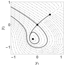
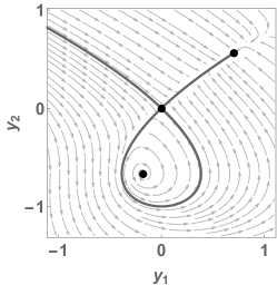
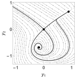
      (d) (50) with $\beta=-1/10$             (e) (50) with $\beta=50/5879$           (f) (50) with $\beta=1/10$

   

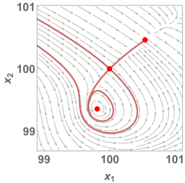
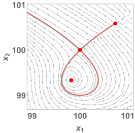
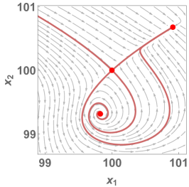
Figure 6: Chemical system undergoing homoclinic bifurcation. Panels (a)–(c) display the state-space for system $(\ref{eq:homoclinic})$ for three different values of $\beta$, where at $\beta=0$ a homoclinic bifurcation takes place. Analogous plots are shown for system $(\ref{eq:homoclinic_g_fixed})$ in panels (d)–(f).

Proof.

Consider the perturbed system

$$\frac{\mathrm{d}z_{1}}{\mathrm{d}t} =\left(\beta-\frac{4}{5}\right)z_{1}+z_{2}-\frac{6}{5}z_{1}z_{2}+\frac{3}{2}z_{2}^{2}+\mu z_{1}\left(z_{2}-\frac{6}{5}z_{1}z_{2}+\frac{3}{2}z_{2}^{2}\right),$$

$$\frac{\mathrm{d}z_{2}}{\mathrm{d}t} =z_{1}-\frac{4}{5}z_{2}-\frac{4}{5}z_{2}^{2}+\mu z_{2}\left(z_{1}-\frac{4}{5}z_{2}^{2}\right),$$ (48)

which is of the form (23) with $q_{1}=(\beta-4/5)z_{1}$ and $q_{2}=-(4/5)z_{2}$. System (45) displays at $\beta=0$ a super-critical homoclinic bifurcation which is generic [21, 6], and therefore robust. Hence, for every sufficiently small $\mu>0$ system (48) displays the same bifurcation at some $\beta=\beta(\mu)$ arbitrarily close to zero. Fixing a sufficiently small $\mu>0$, considering $\beta$ close to zero, and applying translation $x_{1}=(z_{1}+1/\mu)$, $x_{2}=(z_{2}+1/\mu)$, one gets the chemical system

$$\frac{\mathrm{d}x_{1}}{\mathrm{d}t} =\left(\beta-\frac{4}{5}\right)\left(x_{1}-\frac{1}{\mu}\right)+\mu x_{1}\left[\left(x_{2}-\frac{1}{\mu}\right)-\frac{6}{5}\left(x_{1}-\frac{1}{\mu}\right)\left(x_{2}-\frac{1}{\mu}\right)+\frac{3}{2}\left(x_{2}-\frac{1}{\mu}\right)^{2}\right],$$

$$\frac{\mathrm{d}x_{2}}{\mathrm{d}t} =-\frac{4}{5}\left(x_{2}-\frac{1}{\mu}\right)+\mu x_{2}\left[\left(x_{1}-\frac{1}{\mu}\right)-\frac{4}{5}\left(x_{2}-\frac{1}{\mu}\right)^{2}\right],$$ (49)

with the CRN given by (46) with rate coefficients (47). ∎

Let us fix $\mu=1/100$ in (47), so that the resulting chemical system (49) becomes

$$\frac{\mathrm{d}x_{1}}{\mathrm{d}t} =\left(80-100\beta\right)+\left(\frac{141}{5}+\beta\right)x_{1}+\frac{6}{5}x_{1}^{2}-\frac{179}{100}x_{1}x_{2}-\frac{3}{250}x_{1}^{2}x_{2}+\frac{3}{200}x_{1}x_{2}^{2},$$

$$\frac{\mathrm{d}x_{2}}{\mathrm{d}t} =80-\frac{409}{5}x_{2}+\frac{1}{100}x_{1}x_{2}+\frac{8}{5}x_{2}^{2}-\frac{1}{125}x_{2}^{3}.$$ (50)

It is found numerically that (50) undergoes the homoclinic bifurcation at $\beta\approx 50/5879$; the state-space is displayed in Figure 6(d)–(e), and agrees well with that of the target system (45).

Quadratic system. Chemical system (49) is cubic. In Appendix D, we apply a more general quasi-chemical map to design a quadratic chemical system undergoing super-critical homoclinic bifurcation, see Theorem D.1. In particular, quadratic chemical system, with $\beta\in(-1,0)$, given by

$$\frac{\mathrm{d}x_{1}}{\mathrm{d}t} =-10x_{1}+\frac{1}{10}x_{1}x_{2},$$

$$\frac{\mathrm{d}x_{2}}{\mathrm{d}t} =\left(-910+10^{10/3}\right)+(81-10\beta)x_{1}+(10-2\times 10^{4/3})x_{2}+x_{1}^{2}+\left(-1+\frac{\beta}{10}\right)x_{1}x_{2}+\frac{1}{10^{2/3}}x_{2}^{2},$$ (51)

is found numerically to undergo the homoclinic bifurcation at saddle $(10,100)$ when $\beta\approx-191/200$.

8 Discussion

In this paper, we have discussed chemical maps - special transformations that map general dynamical systems into chemical ones, while qualitatively preserving desired dynamical features. We have introduced a novel chemical map, called the quasi-chemical map, which systematically perturbs any given polynomial dynamical system in such a way that it becomes chemical under sufficiently large translations. This map preserves robust dynamical features, such as generic equilibria and limit cycles, temporal properties, such as periods of oscillations, as well as robust bifurcations, such as generic saddle-node and Hopf bifurcations, see Theorem 4.1 in Section 4, Theorem C.1 in Appendix C and Theorem 7.1 in Section 7. Furthermore, the quasi-chemical map increases the degree of polynomial dynamical systems by at most one. These properties make the quasi-chemical map more suitable for experimental implementations e.g. via nucleic acids [5], and more favourable than some alternative transformations, such as the time-change map [11, 12] and the $\mathbf{x}$-factorable map [14]. In particular, while the time-change map preserves trajectories in the state-space, it does not preserve temporal properties; furthermore, it can significantly increase the degree of dynamical systems. On the other hand, while the $\mathbf{x}$-factorable map increases the degree by only one, it is not rigorously justified, and can fail to qualitatively preserve even hyperbolic equilibria, see Section 3. In fact, the quasi-chemical map may be seen as a correction and generalization of the $\mathbf{x}$-factorable map, see Theorem 4.2. For further generalizations of the quasi-chemical map, see Appendix C. Let us note that all of the chemical maps discussed in this paper are dimension-preserving, i.e. these maps do not introduce additional variables. In a follow-up paper, we will focus on dimension-expanding chemical maps that introduce auxiliary variables to achieve chemical systems [6].

In Sections 5–7, we have used the quasi-chemical map to design a number of chemical systems with exotic dynamics and pre-defined bifurcation structures. In particular, in Section 5, we have designed a chemical system with arbitrary many limit cycles. Such systems are of importance to Hilbert’s 16th problem, which asks for the maximum number of limit cycles in two-dimensional $n$-degree polynomial dynamical systems [22]. This number is denoted by $H(n)$, and remains unknown for all $n\geq 2$ [23]. One can pose a similar question in the chemical context: what is the maximum number $H_{\mathcal{C}}(n)$ of limit cycles in two-dimensional $n$-degree chemical systems [7]? The same question restricted to stable limit cycles is also considered in [24], with the corresponding number denoted by $C(n)$. A specific chemical system is designed using time-change and $\mathbf{x}$-factorable maps in [24] which implies a linear lower-bound $C(n)\geq\lfloor(n+2)/6\rfloor$. System (27) from Section 5 predicts a better lower-bound, namely $C(n)\geq\lfloor(n+1)/4\rfloor$. More generally, Theorem B.1 from Appendix B for the time-change map implies that $H_{\mathcal{C}}(n+2)\geq H(n)$; combined with the results from e.g. [25], it follows that the number of limit cycles in chemical systems asymptotically grows as $n^{2}\ln(n)$. Better bounds can be obtained from Theorem 4.1 for the quasi-chemical map, which implies that $H_{\mathcal{C}}(n+1)\geq H(n)$, assuming that only robust limit cycles are counted.

In Section 6, we have designed a cubic chemical system with Lorenz attractor, see Theorem 6.1. A similar system has been put forward in [14]; however, since the $\mathbf{x}$-factorable map is utilized and some of the variables are translated differently, existence of the chaotic attractor is not rigorously justified. In contrast, a chemical system with Lorenz attractor rigorously justified has been put forward in [26]. To design this system, the authors use the time-change map; consequently, the system is quartic and the time-scale at which the Lorenz attractor is tracked is distorted. In Section 6, we have also designed a candidate chaotic chemical system which is quadratic, see Theorem 6.2. In Section 7, we have presented a cubic chemical system undergoing a super-critical homoclinic bifurcation, see Theorem 7.2. This problem has also been considered using the $\mathbf{x}$-factorable map and numerical simulations in [6]. Using a generalized quasi-chemical map, we have also designed a quadratic chemical system undergoing the homoclinic bifurcation, see Theorem D.1.

To close the discussion, we briefly highlight two properties of the quasi-chemical map which are noteworthy for future research. Firstly, the time-change and $\mathbf{x}$-factorable maps introduce equilibria on the boundary of the state-space. As a consequence, when such chemical reaction networks are modelled stochastically, the noise may drive the system to the state-space boundary, thus drastically changing its long-time behavior [27, 7]. On the other hand, chemical system obtained via the quasi-chemical map do not necessarily have equilibria on the boundary of the state-space, and may be less prone to the noise-induced extinctions. Secondly, the quasi-chemical map preserves the degree of some dynamical systems, which leads to an interesting open problem: Find polynomial dynamical systems that can be mapped to chemical ones while preserving both the desired dynamical features and the degree. As a step towards addressing this problem, we present the following result, of which Theorems 5.1 and 6.2 are special cases.

Theorem 8.1.

Consider the polynomial dynamical system

$$\frac{\mathrm{d}y_{i}}{\mathrm{d}t} =\alpha_{i,0}+\sum_{j=1}^{N}\beta_{i,j}y_{j}+\sum_{j=2}^{n_{i}}\gamma_{i,j}y_{i}^{j},\;\;\;\;\;i=1,2,\ldots,N,$$ (52)

where $n_{i}\in\mathbb{Z}_{\geq}$ for all $i=1,2,\ldots,N$. Assume that $\gamma_{i,n_{i}}<0$ if $n_{i}\geq 3$ is odd, and $\gamma_{i,n_{i}}>0$ if $n_{i}\geq 2$ is even for all $i=1,2,\ldots,N$. Then, dynamical system $(\ref{eq:special_case})$ can be mapped to a chemical system of the same degree using the quasi-chemical map $(\ref{eq:quasi_chemical})$.

Proof.

See Appendix C.2. ∎

Appendix A Background theory

In this section, we present further background theory used in this paper.

Definition A.1.

$($Qualitative equivalence$)$ Consider the dynamical system $(\ref{eq:dyn})$ in the state-space region $\mathbb{U}\subset\mathbb{R}^{N}$, and system $(\ref{eq:dyn2})$ in region $\mathbb{V}\subset\mathbb{R}^{N}$. Let $\boldsymbol{\Phi}$ be a continuous map from $\mathbb{U}$ onto $\mathbb{V}$, which has a continuous inverse. Assume that $\boldsymbol{\Phi}$ maps solutions of $(\ref{eq:dyn})$ contained in $\mathbb{U}$ onto the solutions of $(\ref{eq:dyn2})$ contained in $\mathbb{V}$, and preserves the direction of time. Then, dynamical system $(\ref{eq:dyn})$ in $\mathbb{U}$ is said to be qualitatively equivalent to the dynamical system $(\ref{eq:dyn2})$ in $\mathbb{V}$.

Let $\nabla\mathbf{f}(\mathbf{y})\in\mathbb{R}^{N\times N}$ be the Jacobian matrix for (2), where $(\nabla\mathbf{f}(\mathbf{y}))_{i,j}=(\partial f_{i}(\mathbf{y})/\partial y_{j})$. Then, the linearization around the solution $\mathbf{y}(t)$ of (2) is given by

$$\frac{\mathrm{d}\mathbf{z}}{\mathrm{d}t} =\nabla\mathbf{f}(\mathbf{y}(t))\mathbf{z}.$$ (53)

If $\mathbf{y}^{*}$ is a time-independent solution of (2), then $\mathbf{z}(t)=\exp(\nabla\mathbf{f}(\mathbf{y}^{*})t)\mathbf{z}_{0}$, and we associate the eigenvalues of $\nabla\mathbf{f}(\mathbf{y}^{*})$ to $\mathbf{y}^{*}$.

Definition A.2.

$($Equilibrium$)$ $\mathbf{y}^{*}\in\mathbb{R}^{N}$ is a hyperbolic equilibrium for $(\ref{eq:dyn})$ if:

1. $\mathbf{f}(\mathbf{y^{*}})=\mathbf{0}$, and

2. All $N$ eigenvalues associated to $\mathbf{y}^{*}$ have non-zero real parts.

Another important class of solutions of (2) are those that are periodic with period $\tau>0$, which we denote by $\mathbf{y}_{\tau}=\mathbf{y}_{\tau}(t)$. In this case, the solution of the linearization (53) is of the form $\mathbf{z}(t)=P(t)\exp(At)\mathbf{z}_{0}$, where $P(t)\in\mathbb{R}^{N\times N}$ is a $\tau$-periodic matrix, and $A\in\mathbb{R}^{N\times N}$ is time-independent [1]. We say that the eigenvalues of $A$ are characteristic exponents associated $\mathbf{y}_{\tau}(t)$; we note that at least one of the exponents has zero real part.

Definition A.3.

$($Limit cycle$)$ $\mathbf{y}_{\tau}:\mathbb{R}_{\geq}\to\mathbb{R}^{N}$ is a hyperbolic limit cycle of period $\tau>0$ for $(\ref{eq:dyn})$ if:

1. $\mathbf{y}_{\tau}(t)$ is a solution of $(\ref{eq:dyn})$ such that $\mathbf{y}_{\tau}(0)=\mathbf{y}_{\tau}(\tau)$ and $\mathbf{y}_{\tau}(0)\neq\mathbf{y}_{\tau}(t)$ for all $t\in(0,\tau)$, and

2. $(N-1)$ characteristic exponents associated to $\mathbf{y}_{\tau}$ have non-zero real parts.

For solutions $\mathbf{y}(t)$ of (2) that are neither time-independent nor periodic, the associated linearization (53) is more difficult to analyze. In this more general context, particularly important in applications are regions of the state-space on whose boundary the vector field of the dynamical system points inwards. Consequently, if the state of the system is initiated inside such a region, then it stays in there for all future times.

Definition A.4.

$($Trapping region$)$ Let $\mathbb{S}=\{\mathbf{y}\in\mathbb{R}^{N}|V(\mathbf{y})\leq r\textrm{ for some }r>0\}$ be a compact set in the state-space, where $V:\mathbb{R}^{N}\to\mathbb{R}$ is a continuous function. If the vector field $\mathbf{f}(\mathbf{y})$ points inwards on the boundary $V(\mathbf{y})=r$, then $\mathbb{S}$ is called a trapping region for $(\ref{eq:dyn})$.

Appendix B Appendix: Time-change map

Definition B.1.

$($Time-change map$)$ Consider system $(\ref{eq:dyn_components})$. Assume that $f_{i}\in\mathbb{P}_{n}^{\mathcal{N}}(\mathbb{R}^{N};\mathbb{R})$ for $i=1,2,\ldots,K$, and $f_{i}\in\mathbb{P}_{n}^{\mathcal{C}}(\mathbb{R}^{N};\mathbb{R})$ for $i=K+1,K+2,\ldots,N$. Consider the chemical system

$$\frac{\mathrm{d}x_{i}}{\mathrm{d}s} =\left(x_{1}x_{2}\ldots x_{K}\right)f_{i}(\mathbf{x}),\;\;\;i=1,2,\ldots,N.$$ (54)

$\Psi_{s}:\mathbb{P}_{n}^{\mathcal{N}}(\mathbb{R}^{N};\,\mathbb{R}^{N})\to\mathbb{P}_{n+K}^{\mathcal{C}}(\mathbb{R}^{N};\,\mathbb{R}^{N})$, mapping the dynamical system $(\ref{eq:dyn_components})$ to the chemical system $(\ref{eq:timechange})$, is called a time-change map.

The time-change map can be interpreted as a state-dependent change of time-coordinate in $(\ref{eq:dyn_components})$.

Theorem B.1.

Consider system $(\ref{eq:dyn_components})$ with $f_{i}\in\mathbb{P}_{n}^{\mathcal{N}}(\mathbb{R}^{N};\mathbb{R})$ for $i=1,2,\ldots,K$, and $f_{i}\in\mathbb{P}_{n}^{\mathcal{C}}(\mathbb{R}^{N};\mathbb{R})$ for $i=K+1,K+2,\ldots,N$. Assume that $(\ref{eq:dyn_components})$ with initial condition $\mathbf{y}_{0}=(y_{1,0},\ldots,y_{N,0})^{\top}\in\mathbb{R}_{\geq}^{N}$ with $(y_{1,0},\ldots,y_{K,0})^{\top}\in\mathbb{R}_{>}^{K}$ has a solution $\mathbf{y}(t;\mathbf{y}_{0})\in\mathbb{R}_{\geq}^{N}$ with $(y_{1}(t;\mathbf{y}_{0}),\ldots,y_{K}(t;\mathbf{y}_{0}))^{\top}\in\mathbb{R}_{>}^{K}$ for all $t\in[0,t_{0}]$ for some $t_{0}>0$. Then, $(\ref{eq:timechange})$ has the solution $\mathbf{y}(t(s);\mathbf{y}_{0})\in\mathbb{R}_{\geq}^{N}$ for all $s\in[0,\int_{0}^{t_{0}}(y_{1}(\theta;\mathbf{y}_{0})\ldots y_{K}(\theta;\mathbf{y}_{0}))^{-1}\mathrm{d}\theta]$, where $t(s)$ is the inverse of $s(t)=\int_{0}^{t}(y_{1}(\theta;\mathbf{y}_{0})\ldots y_{K}(\theta;\mathbf{y}_{0}))^{-1}\mathrm{d}\theta$.

Proof.

Since $(y_{1}(t;\mathbf{y}_{0}),\ldots,y_{K}(t;\mathbf{y}_{0}))^{\top}\in\mathbb{R}_{>}^{K}$ for all $t\in[0,t_{0}]$, it follows that $s(t)>0$ and $s(t)$ is monotonically increasing for all $t\in[0,t_{0}]$; hence, $s(t)$ has an inverse then, which we denote by $t(s)$. Let $x_{i}(s;\mathbf{y}_{0})=y_{i}(t(s);\mathbf{y}_{0})$; then, it follows from (1) that for all $s\in\left[0,\int_{0}^{t_{0}}\left(y_{1}(\theta;\mathbf{y}_{0})\ldots y_{K}(\theta;\mathbf{y}_{0})\right)^{-1}\mathrm{d}\theta\right]$ variable $x_{i}=x_{i}(s;\mathbf{y}_{0})$ satisfies

$$\frac{\mathrm{d}x_{i}}{\mathrm{d}s} =\frac{\mathrm{d}y_{i}}{\mathrm{d}t}\frac{\mathrm{d}t}{\mathrm{d}s}=\left(x_{1}\ldots x_{K}\right)f_{i}(\mathbf{x}),\;\;\;i=1,2,\ldots,N.$$ (55)

which is identical to (54). ∎

Remark. More generally, monomial $\left(x_{1}x_{2}\ldots x_{K}\right)$ from (54) can be replaced with any other polynomial that ensures (54) is chemical; for example, $\left(x_{1}^{n_{1}}x_{2}^{n_{2}}\ldots x_{K}^{n_{K}}\right)$ with $n_{i}\in\mathbb{Z}_{>}$ is allowed.

Remark. Assume that a solution of (1) is bounded for all $t\geq 0$; then, such a solution can be translated to the positive orthant prior to applying the time-change map. Therefore, Theorem B.1 shows that such translated time-change map can preserve any bounded solution, such as equilibria and limit cycles.

Appendix C Appendix: Quasi-chemical map

In this section, we specialize Theorem 4.1. To this end, we denote the $1$-norm of a vector $\mathbf{x}\in\mathbb{R}^{N}$ by $\|\mathbf{x}\|=|x_{1}|+|x_{2}|+\ldots+|x_{N}|$. Furthermore, we write $\mathbf{x}(\mu)=\mathbf{y}+\mathcal{O}(\mu)$ if $\|\mathbf{x}(\mu)-\mathbf{y}\|\leq c\mu$ for all sufficiently small $\mu>0$, where $c>0$ is a $\mu$-independent constant.

Theorem C.1.

$($Quasi-chemical map: Dynamical properties$)$

1. Finite time-intervals. Let $\mathbf{y}(t)=\mathbf{y}(t;\mathbf{y}_{0})$ be a solution of $(\ref{eq:dyn_components})$ for all $t\in[0,t_{0}]$ for some $t_{0}>0$. Then, for all sufficiently small $\mu$ $(\ref{eq:quasi_chemical})$ has a unique solution $\mathbf{x}(t;\mu)=\mathbf{x}(t;\mu,\mathbf{y}_{0}+\mathbf{T}/\mu)$ for all $t\in[0,t_{0}]$. Furthermore, $\mathbf{x}(t;\mu)=(\mathbf{y}(t)+\mathbf{T}/\mu)+\mathcal{O}(\mu)$ uniformly for $t\in[0,t_{0}]$.

2. Equilibria. Let $\mathbf{y}^{*}$ be a hyperbolic equilibrium of $(\ref{eq:dyn_components})$. Then, for all sufficiently small $\mu$ $(\ref{eq:quasi_chemical})$ has a unique hyperbolic equilibrium $\mathbf{x}^{*}(\mu)$ in a neighborhood of $(\mathbf{y}^{*}+\mathbf{T}/\mu)$. In particular, $\mathbf{x}^{*}(\mu)=(\mathbf{y}^{*}+\mathbf{T}/\mu)+\mathcal{O}(\mu)$. Equilibrium $\mathbf{x}^{*}(\mu)$ is qualitatively equivalent to $\mathbf{y}^{*}$. In particular, eigenvalues $\lambda_{1,\mu},\ldots,\lambda_{N,\mu}$ associated to $\mathbf{x}^{*}(\mu)$ can be ordered so that $\lim_{\mu\to 0}\lambda_{i,\mu}=\lambda_{i,0}$ for all $i=1,\ldots,N$, where $\lambda_{1,0},\ldots,\lambda_{N,0}$ are the eigenvalues associated to $\mathbf{y}^{*}$.

3. Limit cycles. Let $\mathbf{y}_{\tau_{0}}$ be a hyperbolic limit cycle of $(\ref{eq:dyn_components})$ with period $\tau_{0}>0$. Then, for all sufficiently small $\mu$ $(\ref{eq:quasi_chemical})$ has a unique hyperbolic limit cycle $\mathbf{x}_{\tau_{\mu}}$ in a neighborhood of $(\mathbf{y}_{\tau_{0}}+\mathbf{T}/\mu)$. In particular, $\mathbf{x}_{\tau_{\mu}}(t)=(\mathbf{y}_{\tau_{0}}(t)+\mathbf{T}/\mu)+\mathcal{O}(\mu)$ uniformly in time, with period $\tau_{\mu}=\tau_{0}+\mathcal{O}(\mu)$. Limit cycle $\mathbf{x}_{\tau_{\mu}}$ is qualitatively equivalent to $\mathbf{y}_{\tau_{0}}$. In particular, characteristic exponents $\rho_{1,\mu},\ldots,\rho_{N,\mu}$ associated to $\mathbf{x}_{\tau_{\mu}}$ can be ordered so that $\lim_{\mu\to 0}\rho_{i,\mu}=\rho_{i,0}$ for all $i=1,\ldots,N$, where $\rho_{1,0},\ldots,\rho_{N,0}$ are the characteristic exponents associated to $\mathbf{y}_{\tau_{0}}$.

Proof.

The proof follows from (23) and standard theory of differential equations, see e.g. [28]. ∎

Theorem C.1(i) implies the following corollary.

Corollary C.1.

$($Trapping regions$)$ Let $\mathbb{S}_{0}=\{\mathbf{y}\in\mathbb{R}^{N}|V(\mathbf{y})\leq r\textrm{ for some }r>0\}$ be a trapping region for $(\ref{eq:dyn_components})$. Then, $\mathbb{S}_{\mu}=\{\mathbf{x}\in\mathbb{R}^{N}|V(\mathbf{x}-\mathbf{T}/\mu)\leq r\}$ is a trapping region for $(\ref{eq:quasi_chemical})$ for all sufficiently small $\mu>0$.

C.1 Generalized quasi-chemical map

We now present a more general form of the quasi-chemical map. In particular, we generalize Definition 4.1 in three ways: (i) we allow the dependent variables to be scaled with $\mu$ before translations are applied, (ii) we allow translations for different dependent variables to scale differently with respect to $\mu$, and (iii) we allow chemical perturbations to be arbitrary polynomials of degree at most $n$. To this end, we define vector $\mathbf{T}_{\mu,a}=(T_{1}/\mu^{a_{1}},\ldots,T_{N}/\mu^{a_{N}})^{\top}\in\mathbb{R}_{\geq}^{N}$ and diagonal matrix $S_{\mu}=\textrm{diag}(s_{1}/\mu^{b_{1}},\ldots,s_{N}/\mu^{b_{N}})\in\mathbb{R}_{>}^{N\times N}$, where $T_{i}\geq 0$, $s_{i}>0$, and $a_{i},b_{i}\in\mathbb{Z}$ are fixed parameters, while $\mu>0$ is a free parameter.

Definition C.1.

$($Quasi-chemical map$)$ Consider system $(\ref{eq:dyn_components})$. Consider also system

$$\frac{\mu^{b_{i}}}{s_{i}}\frac{\mathrm{d}x_{i}}{\mathrm{d}t} =\left[q_{i}\left(S_{\mu}^{-1}(\mathbf{x}-\mathbf{T}_{\mu,\mathbf{a}})\right)+p_{i}\left(S_{\mu}^{-1}(\mathbf{x}-\mathbf{T}_{\mu,\mathbf{a}});\mu\right)\right]+\frac{\mu^{a_{i}}}{T_{i}}x_{i}\Big{[}f_{i}\left(S_{\mu}^{-1}(\mathbf{x}-\mathbf{T}_{\mu,\mathbf{a}})\right)-q_{i}\left(S_{\mu}^{-1}(\mathbf{x}-\mathbf{T}_{\mu,\mathbf{a}})\right)\Big{]},$$ (56)

for all $i=1,2,\ldots,N$, where $p_{i}(\cdot;\mu)\in\mathbb{P}_{n}(\mathbb{R}^{N},\mathbb{R})$ are polynomials such that $p_{i}(\mathbf{z};0)=0$. Assume that all $[q_{i}(S_{\mu}^{-1}(\mathbf{x}-\mathbf{T}_{\mu,\mathbf{a}}))+p_{i}(S_{\mu}^{-1}(\mathbf{x}-\mathbf{T}_{\mu,\mathbf{a}});\mu)]\in\mathbb{P}_{n}^{\mathcal{C}}(\mathbb{R}^{N},\mathbb{R})$ are chemical for all sufficiently small $\mu>0$. Assume also that $a_{i}>b_{i}$ for all $i=1,2,\ldots,N$. Then, $\Psi_{\mu}:\mathbb{P}_{n}(\mathbb{R}^{N},\mathbb{R}^{N})\to\mathbb{P}_{n+1}^{\mathcal{C}}(\mathbb{R}^{N},\mathbb{R}^{N})$, mapping the dynamical system $(\ref{eq:dyn_components})$ to the chemical system $(\ref{eq:quasi_chemical_g})$ for all sufficiently small $\mu>0$, is called a quasi-chemical map.

Remark. Definition C.1 can be further generalized by replacing the diagonal matrix $S_{\mu}\in\mathbb{R}^{N\times N}$ with general matrix $A_{\mu}\in\mathbb{R}^{N\times N}$ that is non-singular for all sufficiently small $\mu>0$.

Under affine change of coordinates $z_{i}=(\mu^{b_{i}}/s_{i})(x_{i}-T_{i}/\mu^{a_{i}})$, system (56) becomes

$$\frac{\mathrm{d}z_{i}}{\mathrm{d}t} =f_{i}(\mathbf{z})+p_{i}(\mathbf{z};\mu)+\mu^{a_{i}-b_{i}}\frac{s_{i}}{T_{i}}z_{i}\left[f_{i}(\mathbf{z})-q_{i}(\mathbf{z})\right],\;\;\;i=1,2,\ldots,N.$$ (57)

It follows from (57) and the assumption $a_{i}>b_{i}$ that the quasi-chemical map from Definition C.1 preserves robust dynamical features, i.e. satisfies an analogue of Theorem 4.1. Furthermore, Theorem C.1 also holds, but with a different error estimates, namely $\mathcal{O}(\mu^{\kappa})$, where $\kappa>0$ is the minimum value in $\{a_{1}-b_{1},a_{2}-b_{2},\ldots,a_{N}-b_{N}\}$.

To obtain an analogue of (25), we choose $q_{i}=p_{i}=0$ in (56), leading to

$$\frac{\mathrm{d}x_{i}}{\mathrm{d}t} =\mu^{a_{i}-b_{i}}\frac{s_{i}}{T_{i}}x_{i}f_{i}\left(S_{\mu}^{-1}(\mathbf{x}-\mathbf{T}_{\mu,\mathbf{a}})\right),\;\;\;i=1,2,\ldots,N.$$ (58)

      (a) (59) with $\mu=1/100$          (b) (59) with $\mu=1/1000$         (c) (59) with $\mu=1/1000$

       

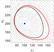
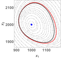
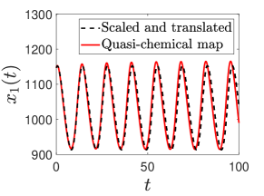
Figure 7: Application of the generalized quasi-chemical map (56) on dynamical system (15). Panel (a) displays state-space for system $(\ref{eq:ex_QF_3})$ with $\mu=1/100$, with the limit cycle shown as the solid red curve, and the equilibrium as the blue dot; also shown as dashed black curve is the limit cycle of $(\ref{eq:ex1})$ under the same scaling and translation as in $(\ref{eq:ex_QF_3})$. Panel (b) displays the same plot for $\mu=1/1000$, while panel (c) displays a corresponding time-state space.

Example. Let us apply on system (15) the quasi-chemical map (56) with $q_{1}=p_{1}=0$, $q_{2}=f_{2}$, $p_{2}=0$, $T_{1}=1$, $T_{2}=2$, $a_{1}=a_{2}=1$, $s_{1}=s_{1}=1$ and $b_{1}=b_{2}=1/2$, which leads to

$$\frac{\mathrm{d}x_{1}}{\mathrm{d}t} =\mu x_{1}\left[\frac{1}{2}\left(x_{2}-\frac{2}{\mu}\right)+\frac{1}{8}\left(x_{1}-\frac{1}{\mu}\right)\right],$$

$$\frac{\mathrm{d}x_{2}}{\mathrm{d}t} =-\frac{1}{2}\left(x_{1}-\frac{1}{\mu}\right)-\mu^{1/2}\frac{1}{20}\left(x_{1}-\frac{1}{\mu}\right)\left(x_{2}-\frac{2}{\mu}\right)+\mu^{1/2}\frac{1}{20}\left(x_{2}-\frac{2}{\mu}\right)^{2}-\frac{3}{32}\left(x_{2}-\frac{2}{\mu}\right).$$ (59)

One can readily show that (59) is chemical for all sufficiently small $\mu>0$. In Figure 7(a), we display the state-space for (59) when $\mu=1/100$. Analogous plot is shown in Figure 7(b) for $\mu=1/1000$, with a corresponding time-state space shown in Figure 7(c). These plots confirm that the limit cycle is now of order $\mathcal{O}(\mu^{-1/2})$, as opposed to $\mathcal{O}(1)$ as in Figure 2. Let us note that the error between the limit cycle of system (59) and that of suitably scaled and translated target system, as well as their periods, is $\mathcal{O}(\mu^{1/2})$, as opposed to $\mathcal{O}(\mu)$ as in Figure 2; in particular, the convergence order is now lower due to the magnification of the limit cycle.

C.2 Proof of Theorem 8.1

In what follows, we use the convention that if $b<a$, then $\sum_{i=a}^{b}f_{i}=0$ for every sequence $f_{i}$.

Proof.

Assume first that the $i$th equation from $(\ref{eq:special_case})$ has $n_{i}\leq 1$, i.e. that this equation is linear. Then, applying the quasi-chemical map of the form (24) with $q_{i}=c_{i}\geq 0$, one obtains

$$\frac{\mathrm{d}x_{i}}{\mathrm{d}t} =c_{i}+\frac{\mu}{T_{i}}x_{i}\left[\alpha_{i,0}+\sum_{j=1}^{N}\beta_{i,j}\left(x_{j}-\frac{T_{j}}{\mu}\right)-c_{i}\right].$$ (60)

Assume now that $n_{i}\geq 2$. Then, the zero-degree term in $\sum_{j=2}^{n_{i}}\gamma_{i,j}\left(x_{i}-T_{i}/\mu\right)^{j}$ is dominated by $\gamma_{i,n_{i}}(-T_{i}/\mu)^{n_{i}}>0$ as $\mu\to 0$; therefore, $q_{i}(x_{i})=\alpha_{i,0}+\beta_{i,i}\left(x_{i}-T_{i}/\mu\right)+\sum_{j=2}^{n_{i}}\gamma_{i,j}\left(x_{i}-T_{i}/\mu\right)^{j}$ is quasi-chemical. Applying the quasi-chemical map (24) with this choice of $q_{i}(x_{i})$, one obtains

$$\frac{\mathrm{d}x_{i}}{\mathrm{d}t} =\alpha_{i,0}+\beta_{i,i}\left(x_{i}-\frac{T_{i}}{\mu}\right)+\sum_{j=2}^{n_{i}}\gamma_{i,j}\left(x_{i}-\frac{T_{i}}{\mu}\right)^{j}+\frac{\mu}{T_{i}}x_{i}\left[\sum_{j=1,j\neq i}^{N}\beta_{i,j}\left(x_{j}-\frac{T_{j}}{\mu}\right)\right].$$ (61)

∎

Remark. Depending on the sign of some of the coefficients, further simplifications are possible in (60) and (61).

Appendix D Appendix: Homoclinic bifurcation

In what follows, we use the quasi-chemical map (56) on the dynamical system

$$\frac{\mathrm{d}y_{1}}{\mathrm{d}t} =y_{2},$$

$$\frac{\mathrm{d}y_{2}}{\mathrm{d}t} =y_{1}+\beta y_{2}+y_{1}^{2}-y_{1}y_{2},$$ (62)

which undergoes a super-critical homoclinic bifurcation [1][Chapter 4.8].

Theorem D.1.

$($Quadratic chemical system undergoing super-critical homoclinic bifurcation$)$ Consider the CRN

$$X_{1} \xrightarrow[]{\alpha_{1}}\varnothing,\;\;\;X_{1}+X_{2}\xrightarrow[]{\alpha_{2}}2X_{1}+X_{2},\;\;\;\varnothing\xrightleftharpoons[\alpha_{4}]{\alpha_{3}}X_{2},\;\;\;X_{1}\xrightarrow[]{\alpha_{5}}X_{1}+X_{2},$$

$$2X_{1} \xrightarrow[]{\alpha_{6}}2X_{1}+X_{2},\;\;\;X_{1}+X_{2}\xrightarrow[]{\alpha_{7}}X_{1},\;\;\;2X_{2}\xrightarrow[]{\alpha_{8}}3X_{2}.$$ (63)

Assume that the rate coefficients are given by

$$\alpha_{1} =\frac{1}{\mu^{1/2}},\;\;\;\alpha_{2}=\mu^{1/2},\;\;\;\alpha_{3}=\frac{1}{\mu^{5/3}}-\frac{1}{\mu^{3/2}}+\frac{1}{\mu}-\frac{1}{\mu^{1/2}},\;\;\;\alpha_{4}=\frac{2}{\mu^{2/3}}-\frac{1}{\mu^{1/2}},$$

$$\alpha_{5} =\frac{1}{\mu}-\frac{2+\beta}{\mu}+1,\;\;\;\alpha_{6}=1,\;\;\;\alpha_{7}=1-\beta\mu^{1/2},\;\;\;\alpha_{8}=\mu^{1/3}.$$ (64)

Then, for every sufficiently small $\mu>0$, CRN $(\ref{eq:homoclinic_CRN2})$ undergoes a super-critical homoclinic bifurcation at saddle $(1/\mu^{1/2},1/\mu)\in\mathbb{R}_{>}^{2}$ at some parameter value $\beta=\beta(\mu)\in(-1,0)$.

Proof.

Consider the perturbed system

$$\frac{\mathrm{d}z_{1}}{\mathrm{d}t} =f_{1}(z_{1},z_{2})=z_{2}+\mu^{1/2}z_{1}z_{2},$$

$$\frac{\mathrm{d}z_{2}}{\mathrm{d}t} =f_{2}(z_{1},z_{2})=z_{1}+\beta\left(z_{2}+\mu^{1/2}z_{1}z_{2}\right)+z_{1}^{2}-z_{1}z_{2}+\mu^{1/3}z_{2}^{2},$$ (65)

which is of the form (57) with $q_{1}=p_{1}=0$, $q_{2}=f_{2}$ and $p_{2}=\mu^{1/2}z_{1}z_{2}+\mu^{1/3}z_{2}^{2}$. The angle between the vector field of (65) and the $z_{1}$-axis is given by $\theta=\tan^{-1}[f_{1}(z_{1},z_{2})/f_{2}(z_{1},z_{2})]$, and satisfies the differential equation

$$\frac{\mathrm{d}\theta}{\mathrm{d}\beta} =\frac{f_{1}^{2}(z_{1},z_{2})}{f_{1}^{2}(z_{1},z_{2})+f_{2}^{2}(z_{1},z_{2})}.$$ (66)

Hence, for points in the state-space which are not equilibria, the vector field rotates anti-clockwise as parameter $\beta$ is increased. If $\mu=0$, then (65) has a stable hyperbolic limit cycle with clock-wise orientation for a range of values $\beta>-1$ [1][Chapter 4.8]; hence, the same is true for (65) for all sufficiently small $\mu>0$. It follows from (66) and [1][Chapter 4.6] that this limit cycle monotonically expands as $\beta$ is increased, until it forms a stable homoclinic loop at the saddle $(0,0)$ at some bifurcation value $\beta(\mu)>-1$. Since the homoclinic loop is stable, it follows that the trace of Jacobian for (65) at $(0,0)$ is negative at the bifurcation, i.e. $\beta(\mu)<0$ [1][Chapter 4.8]. Choosing a sufficiently small $\mu>0$, restricting $\beta\in(-1,0)$, and applying translation $x_{1}=(z_{1}+1/\mu^{1/2})$ and $x_{2}=(z_{2}+1/\mu)$, system (65) becomes

$$\frac{\mathrm{d}x_{1}}{\mathrm{d}t} =\mu^{1/2}x_{1}\left(x_{2}-\frac{1}{\mu}\right),$$

$$\frac{\mathrm{d}x_{2}}{\mathrm{d}t} =\left(x_{1}-\frac{1}{\mu^{1/2}}\right)+\beta\left[\left(x_{2}-\frac{1}{\mu}\right)+\mu^{1/2}\left(x_{1}-\frac{1}{\mu^{1/2}}\right)\left(x_{2}-\frac{1}{\mu}\right)\right]+\left(x_{1}-\frac{1}{\mu^{1/2}}\right)^{2}$$

$$-\left(x_{1}-\frac{1}{\mu^{1/2}}\right)\left(x_{2}-\frac{1}{\mu}\right)+\mu^{1/3}\left(x_{2}-\frac{1}{\mu}\right)^{2},$$ (67)

with the CRN given by (63)–(64). ∎

Fixing $\mu=1/100$ in (67), one obtains (51).

Appendix E Appendix: Perturbed harmonic oscillator

Lemma E.1.

Consider the perturbed harmonic oscillator given by $(\ref{eq:HO_1})$. Let $0<r_{1}<r_{2}<\ldots<r_{n}$ be arbitrary real numbers. Then, there exists coefficients $\beta_{i}=\beta_{i}(r_{1},r_{2},\ldots,r_{N})$ for $i=0,1,\ldots,N$ such that for every sufficiently small $\varepsilon>0$ system $(\ref{eq:HO_1})$ has $n$ limit cycles. The $i$th limit cycle is arbitrarily close to $y_{1}(t)=r_{i}\cos(t)$ and $y_{2}(t)=-r_{i}\sin(t)$, and has period arbitrarily close $2\pi$. The $n$th limit cycle is stable, and the limit cycles alternate in stability.

Proof.

Substituting $f_{1}=\beta_{0}y_{1}+\beta_{1}y_{1}^{3}+\beta_{2}y_{1}^{5}+\ldots+\beta_{n}y_{1}^{2n+1}$ and $f_{2}=0$ into

$$I(r) =\int_{0}^{2\pi}\Big{[}f_{1}(r\cos(s),-r\sin(s))\cos(s)-f_{2}(r\cos(s),-r\sin(s))\sin(s)\Big{]}\mathrm{d}s,$$

one obtains

$$I(r) =\pi r\sum_{i=0}^{n}2^{-2i}\binom{2i+1}{i+1}\beta_{i}r^{2i},$$ (68)

where we use the fact that $\int_{0}^{2\pi}\cos^{2n}(t)\mathrm{d}t=2^{-2n+2}\binom{2n-1}{n}\pi$. Using Vieta’s formulas, it follows that $0<r_{1}^{2}<r_{2}^{2}<\ldots<r_{n}^{2}$ are the roots of $I(r)$ if

$$\beta_{i} =(-1)^{n-i+1}2^{2i}\binom{2i+1}{i+1}^{-1}\sum_{l\in C_{n-i}^{n}}\left(r_{l(1)}r_{l(2)}\ldots r_{l(n-i)}\right)^{2}\;\;\;\textrm{for all }i=0,1,2,\ldots,n-1,$$

$$\beta_{n} =-2^{2n}\binom{2n+1}{n+1}^{-1},$$ (69)

where $C_{k}^{n}$ denotes the set of all combinations of length $1\leq k\leq n$ of the elements from $\{1,2,\ldots,n\}$. Note that we impose $2^{-2n}\binom{2n+1}{n+1}\beta_{n}<0$ to ensure stability of the limit cycle with radius $r_{n}$; we arbitrarily let $2^{-2n}\binom{2n+1}{n+1}\beta_{n}=-1$. Simple zeros of $I(r)$ correspond to the hyperbolic limit cycles of (26), and their stability is determined by the slope of $I(r)$ [1][Chapter 4.9], implying the statement of the lemma. ∎

Rate coefficients for (27). The coefficients are given by

$$\alpha_{i} =\left|\delta_{0}(i)\frac{1}{\mu}+\varepsilon\sum_{j=0}^{n}\beta_{j}\binom{2j+1}{i}\left(\frac{1}{\mu}\right)^{2j+1-i}\right|,\;\;i=0,1,\ldots,2n+1,\;\;\alpha_{2n+2}=1,\;\;\alpha_{2n+3}=\mu,$$ (70)

where $\beta_{0},\beta_{1},\ldots,\beta_{n}$ are given by $(\ref{eq:HO_1_b})$, and $\delta_{i}(j)$ be the Kronecker-delta such that $\delta_{i}(j)=1$ if $j=i$, and $\delta_{i}(j)=0$ otherwise.

References

- [1] Perko, L., 2001. Differential Equations and Dynamical Systems. 3rd Edition, Springer-Verlag.
- [2] Feinberg, M. Lectures on chemical reaction networks. Delivered at the Mathematics Research Center, University of Wisconsin, 1979.
- [3] Érdi, P., Tóth, J. Mathematical models of chemical reactions. Theory and applications of deterministic and stochastic Models. Manchester University Press, Princeton University Press, 1989.
- [4] Endy D., 2005. Foundations for engineering biology. Nature, 484: 449–453.
- [5] Soloveichik, D., Seeing G., Winfree E., 2010. DNA as a universal substrate for chemical kinetics. Proceedings of the National Academy of Sciences, 107(12): 5393–5398.
- [6] Plesa, T., Vejchodský, T., and Erban, R., 2016. Chemical reaction systems with a homoclinic bifurcation: An inverse problem. Journal of Mathematical Chemistry, 54(10): 1884–1915.
- [7] Plesa, T., Vejchodský, T., and Erban, R, 2017. Test models for statistical inference: Two-dimensional reaction systems displaying limit cycle bifurcations and bistability, 2017. Stochastic Dynamical Systems, Multiscale Modeling, Asymptotics and Numerical Methods for Computational Cellular Biology.
- [8] Plesa, T., and Zygalakis, K. C., Anderson, D. F., and Erban, R., 2018. Noise control for molecular computing. Journal of the Royal Society Interface, 15(144): 20180199.
- [9] T. Plesa, G. B. Stan, T. E. Ouldridge, and W. Bae., 2021. Quasi-robust control of biochemical reaction networks via stochastic morphing. Journal of the Royal Society Interface, 18: 1820200985.
- [10] Plesa, T., Dack, A., and Ouldridge, T. E., 2023. Integral feedback in synthetic biology: Negative-equilibrium catastrophe. Journal of Mathematical Chemistry, 61: 1980–2018.
- [11] Figueiredo, A., Gleria, I.M., Rocha, T.M., 2000. Boundedness of solutions and Lyapunov functions in quasi-polynomial systems. Phys. Lett. A, 268: 335–341.
- [12] Hangos, K.M., Szederkényi, G., 2011. Mass action realizations of reaction kinetic system models on various time scales. J. Phys.: Conf. Ser., 268: 012009.
- [13] Plesa, T., 2023. Stochastic approximations of higher-molecular by bi-molecular reactions. Journal of Mathematical Biology, 86(2): 28.
- [14] Samardzija, N., Greller, L.D., Wasserman, E., 1989. Nonlinear chemical kinetic schemes derived from mechanical and electrical dynamical systems. J. Chem. Phys. 90: 2296–2304.
- [15] Kuznetsov, Y. A., 1998. Elements of applied bifurcation theory. Springer, Berlin.
- [16] Escher, C., 1981. Bifurcation and coexistence of several limit cycles in models of open two-variable quadratic mass-action systems. Chem. Phys., 63(3):337–348.
- [17] Eckweiler, H. J., 1946. Nonlinear differential equations of the van der Pol type with a variety of periodic solutions. Studies in Nonlinear Vibration Theory, Institute of Mathematics and Mechanics, New York University.
- [18] Lorenz, E. N., 1963. Deterministic nonperiodic flow. Journal of Atmospheric Sciences, 20(2): 130–141.
- [19] Tucker, W., 1999. The Lorenz attractor exists. Comptes Rendus de l’Académie des Sciences-Series I-Mathematics, 328(12): 1197–1202.
- [20] Sprott, J. C., 1994. Some simple chaotic flows. Phys. Rev. E, 50, R647(R).
- [21] Sandstede, B., 1997. Constructing dynamical systems having homoclinic bifurcation points of codimension two. Journal of Dynamics and Differential Equations, Vol. 9, No. 2., 4: 296–288.
- [22] Hilbert, D., 1902. Mathematical problems. Bulletin of the American Mathematical Society, 80: 437–479.
- [23] Ilyashenko, Y., 2002. Centennial history of Hilbert’s 16th problem. Bulletin of the American Mathematical Society, 39(3): 301–354.
- [24] Erban, R., Kang, H.W., 2023. Chemical Systems with Limit Cycles. Bull Math Biol 85, 76.
- [25] Christopher, C.J., and Lloyd, N.G., 1995. Polynomial Systems: A Lower Bound for the Hilbert Numbers. Proceedings: Mathematical and Physical Sciences, 450: 219–224.
- [26] Susits, M., Tóth, J., 2024. Rigorously proven chaos in chemical kinetics. Available as: https://arxiv.org/abs/2402.18523.
- [27] Vellela, M., Qian, H., 2007. A quasistationary analysis of a stochastic chemical reaction: Keizers Paradox. Bulletin of Mathematical Biology, 69: 1727–1746.
- [28] Coddington, A. and Levinson, N. Theory of Ordinary Differential Equations. McGraw-Hill, New-York, 1955.