Fast randomized least-squares solvers can be just as accurate and stable as classical direct solvers

Abstract

One of the greatest success stories of randomized algorithms for linear algebra has been the development of fast, randomized algorithms for highly overdetermined linear least-squares problems. However, none of the existing algorithms is backward stable, preventing them from being deployed as drop-in replacements for existing QR-based solvers. This paper introduces FOSSILS, a fast, provably backward stable randomized least-squares solver. FOSSILS combines iterative refinement with a preconditioned iterative method applied to the normal equations, and it converges at the same rate as existing randomized least-squares solvers. This work offers the promise of incorporating randomized least-squares solvers into existing software libraries while maintaining the same level of accuracy and stability as classical solvers.

1 Motivation

In recent years, researchers in the field of randomized numerical linear algebra (RNLA) have developed a suite of randomized methods for linear algebra problems such as linear least-squares [Sar06, RT08, AMT10, PW16] and low-rank approximation [DDH07, HMT11, TW23].

We will study randomized algorithms for the overdetermined linear least-squares problem:

$$\boldsymbol{x}=\operatorname*{argmin}_{\boldsymbol{x}\in^{n}}\left\|\boldsymbol{b}-\boldsymbol{A}\boldsymbol{x}\right\|\quad\text{where }\boldsymbol{A}\in^{m\times n},\>\boldsymbol{b}\in^{m},\>m\geq n.$$ (1.1)

Here, and throughout, $\left\|\cdot\right\|$ denotes the Euclidean norm of a vector or the spectral norm of a matrix. The classical method for solving 1.1 requires a QR decomposition of $\boldsymbol{A}$ at $\mathcal{O}(mn^{2})$ cost. For highly overdetermined problems, with $m\gg n$, RNLA researchers have developed methods for solving 1.1 which require fewer than $\mathcal{O}(mn^{2})$ operations. Indeed, in exact arithmetic, sketch-and-precondition methods [RT08, AMT10] and iterative sketching methods [PW16, OPA19, LP21, Epp24] both solve 1.1 to high accuracy in roughly $\mathcal{O}(mn+n^{3})$ operations, a large improvement over the classical method if $m\gg n\gg 1$, and much closer to the theoretical lower bound of $\Omega(mn)$. Despite these seemingly attractive algorithms, programming environments such as MATLAB, numpy, and scipy still use classical QR-based methods to solve 1.1, even for problems with $m\gg n\gg 1$. This prompts us to ask:

Replacing an existing solver in MATLAB or numpy, each of which have millions of users, should only be done with strong assurances that the new solver is just as accurate and reliable as the previous method. The classic (Householder) QR-based least-squares method is backward stable:

Definition 1.1 (Backward stability).

A least-squares solver is backward stable if the numerically computed solution $\boldsymbol{\widehat{x}}$ is the exact solution to a slightly perturbed problem

$$\boldsymbol{\widehat{x}}=\operatorname*{argmin}_{\boldsymbol{\widehat{x}}\in^{n}}\left\|(\boldsymbol{b}+\boldsymbol{\Delta b})-(\boldsymbol{A}+\boldsymbol{\Delta A})\boldsymbol{\widehat{x}}\right\|\quad\text{where }\left\|\boldsymbol{\Delta A}\right\|\lesssim\left\|\boldsymbol{A}\right\|u,\>\left\|\boldsymbol{\Delta b}\right\|\lesssim\left\|\boldsymbol{b}\right\|u.$$ (1.2)

Here, and going forward, the symbol $A\lesssim B$ indicates that $A\leq C(m,n)B$ for a polynomial prefactor $C(m,n)$ and $u$ denotes the unit roundoff ($u\approx 10^{-16}$ in double precision). To replace QR-based least-squares solvers in general-purpose software, we need a randomized least-squares solver that is also backward stable.

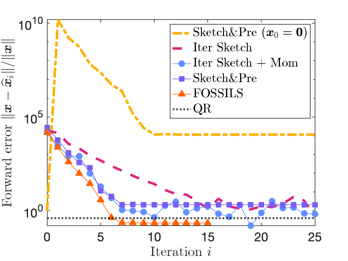
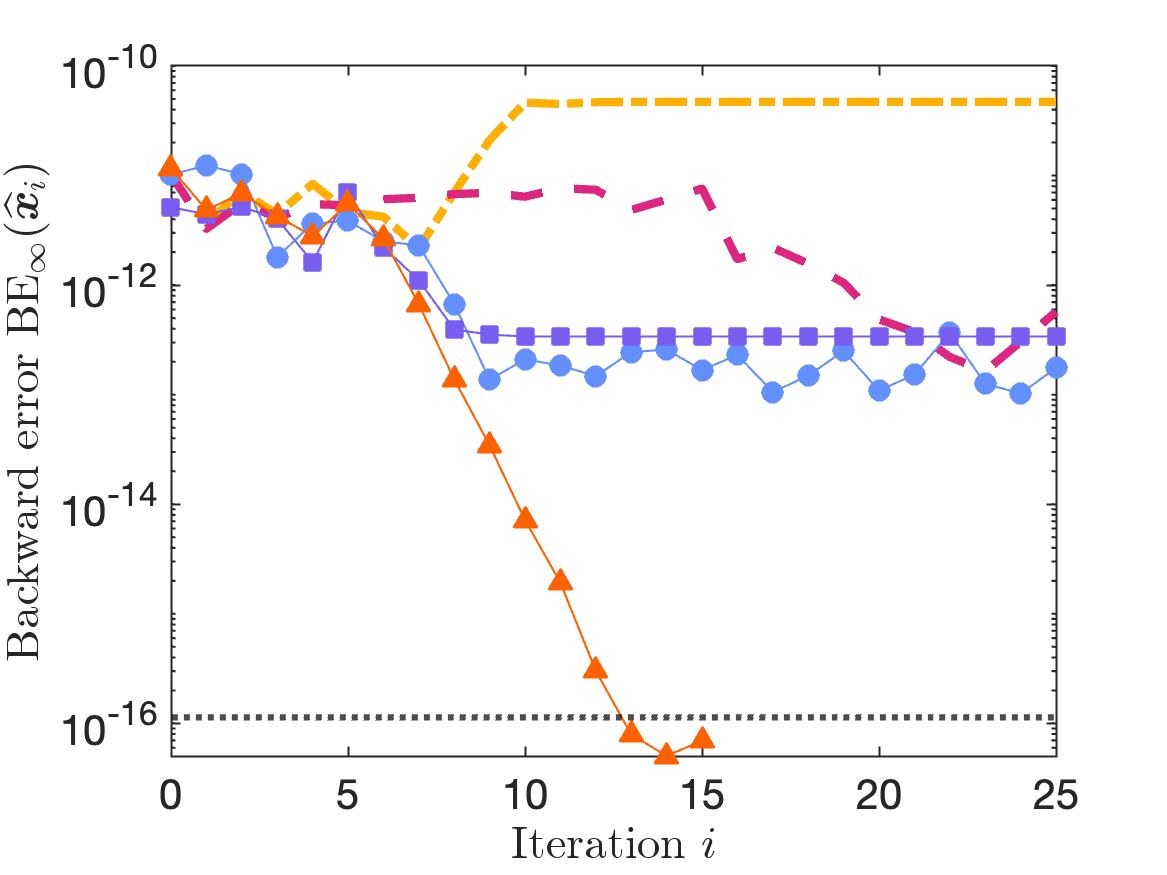
Figure 1: Forward error (left) and backward error (right, 3.5) for different randomized least-squares solvers. A reference accuracy for Householder QR is shown as a dashed line. All of the randomized methods, except sketch-and-precondition with the zero initialization, are forward stable (achieving comparable forward error to Householder QR), but only FOSSILS is backward stable.

Unfortunately, existing fast, randomized least-squares solvers are not backward stable, as demonstrated in Fig. 1. We test two existing solvers, each with two variants:

• Sketch-and-precondition with both the zero initialization (yellow dot-dashed) and sketch-and-solve initialization (purple squares)

• Iterative sketching with (blue circles) and without (pink dashed) momentum acceleration.

We test on a $4000\times 50$ random least-squares problem with residual norm $\left\|\boldsymbol{b}-\boldsymbol{A}\boldsymbol{x}\right\|=10^{-6}$ and condition number $\kappa\coloneqq\operatorname{cond}(\boldsymbol{A})\coloneqq\sigma_{\rm max}(\boldsymbol{A})/\sigma_{\rm min}(\boldsymbol{A})=10^{12}$. We generated these problems with a matrix $\boldsymbol{A}$ with logarithmically spaced singular values and Haar random singular vectors, the solution $\boldsymbol{x}$ is a uniformly random unit vector, and the residual $\boldsymbol{b}-\boldsymbol{A}\boldsymbol{x}$ is uniformly random with the specified norm; see [Epp24, sec. 1.1.1] for details. All randomized methods use a sparse sign embedding with dimension of $d=20n$ (see section 2.1).

Looking first at the left panel of Fig. 1, we see all of these methods—except sketch-and-precondition with the zero initialization—are empirically forward stable, achieving roughly the same forward error $\left\|\boldsymbol{x}-\boldsymbol{\widehat{x}}\right\|$ as the solution by QR factorization. However, none of the existing fast, randomized methods is backward stable. This is demonstrated in the right panel of Fig. 1, which shows that the backward error of all existing randomized methods fails to match the backward error of QR. (The backward error is a measure of the minimal size of the perturbations $\boldsymbol{\Delta A},\boldsymbol{\Delta b}$ needed to satisfy 1.2; see 3.5 for a formal definition of the backward error.)

As existing randomized least-squares solvers are not backward stable, they are not appropriate as replacements for QR-based solvers in general software, at least not for all least-squares problems. This motivates us to address the following question, originally raised in [MNTW24]:

In this article, we answer this question in the affirmative by introducing FOSSILS (Fast Optimal Stable Sketchy Iterative Least Squares), a provably backward stable randomized least-squares solver with a fast $\widetilde{\mathcal{O}}(mn+n^{3})$ runtime.

The fast convergence and stability of FOSSILS are shown in the orange triangle curves in Fig. 1. In the left panel, we see that FOSSILS converges to the maximum attainable forward error $\left\|\boldsymbol{x}-\boldsymbol{\widehat{x}}\right\|$ at the same rate to both sketch-and-precondition and iterative sketching with momentum. In the right panel, we see that the backward error of FOSSILS continues to drop past the point where other methods stagnate, converging to the same backward error as the QR-based method.

1.1 Outline

The rest of this paper is organized as follows. Section 2 discusses background on randomized least-squares solvers and recent efforts to understand their stability. Section 3 introduces the FOSSILS method (section 3.1) and provides implementation guidance (section 3.4). Section 4 presents numerical experiments, and section 5 presents our proof of backward stability of FOSSILS. We conclude in section 6 by generalizing our analysis to a broader class of algorithms (section 6.1) and discussing implications of our analysis for the stability of the sketch-and-precondition method (section 6.2).

1.2 Notation

The relation $A\lesssim B$ or $B\gtrsim A$ indicate that $A\leq C(m,n)B$ for a prefactor $C(m,n)$ that is a polynomial function of $m$ and $n$. If $A\lesssim B$ and $B\lesssim A$, we write $A\asymp B$. The symbol $u$ denotes the unit roundoff, roughly equal to $2\times 10^{-16}$ in double precision arithmetic.

The (spectral norm) condition number of a matrix $\boldsymbol{B}$ is $\operatorname{cond}(\boldsymbol{B})\coloneqq\sigma_{\rm max}(\boldsymbol{B})/\sigma_{\rm min}(\boldsymbol{B})$. We reserve the symbol $\kappa$ for the condition number of $\boldsymbol{A}$, $\kappa\coloneqq\operatorname{cond}(\boldsymbol{A})$. The double lines $\left\|\cdot\right\|$ indicate the $\ell_{2}$ norm of a vector or spectral norm of a matrix; $\left\|\cdot\right\|_{\rm F}$ is the Frobenius norm.

2 Background and related work

This section provides an overview of existing fast randomized least-squares solvers and their stability properties. We begin in section 2.1 by discussing sketching, the core tool that will power all of the algorithms we will discuss. The following subsections discuss three classes of randomized least-squares solvers: sketch-and-solve (section 2.2), sketch-and-precondition (section 2.3), and iterative sketching (section 2.4). Section 2.5 discusses existing work on the stability of these algorithms.

2.1 Sketching

The core ingredient to most randomized least-squares solvers is sketching.

Definition 2.1 (Sketching matrix).

A (random) matrix $\boldsymbol{S}\in^{d\times m}$ is called a sketching matrix or subspace embedding for a matrix $\boldsymbol{A}$ with distortion $0<\eta<1$ if

$$(1-\eta)\left\|\boldsymbol{A}\boldsymbol{y}\right\|\leq\left\|\boldsymbol{S}(\boldsymbol{A}\boldsymbol{y})\right\|\leq(1+\eta)\left\|\boldsymbol{A}\boldsymbol{y}\right\|\quad\text{for all }\boldsymbol{y}\in^{n}.$$ (2.1)

Most constructions for sketching matrices $\boldsymbol{S}$ are probabilistic, in which case we demand that 2.1 holds with high probability over the randomness in $\boldsymbol{S}$.

Typically, we require the output dimension $d$ to be much smaller than the number of rows $m$ of $\boldsymbol{A}$, so $\boldsymbol{S}$ acts to reduce high-dimensional vectors $\boldsymbol{z}\in^{m}$ to low-dimensional vectors $\boldsymbol{S}\boldsymbol{z}\in^{d}$ while approximately preserving the lengths of vectors of the form $\boldsymbol{z}=\boldsymbol{A}\boldsymbol{y}$.

For computational efficiency, we will need access to sketching matrices which are rapid to apply to a vector, of which there are many [MT20, sec. 9]. In our experiments, we will make use of sparse sign embeddings [MT20, sec. 9.2]. A sparse sign embedding is a matrix

$$\boldsymbol{S}=\zeta^{-1/2}\begin{bmatrix}\boldsymbol{s}_{1}&\cdots&\boldsymbol{s}_{m}\end{bmatrix},$$

where $\boldsymbol{s}_{1},\ldots,\boldsymbol{s}_{m}\in^{m}$ are independent random vectors with exactly $\zeta$ nonzero entries in uniformly random positions. The nonzero entries of $\boldsymbol{s}_{i}$ take the values $\pm 1$ with equal probability. Cohen [Coh16] showed that a sparse sign embedding is a sketching matrix for $\boldsymbol{A}\in^{m\times n}$ provided

$$d\geq\mathrm{const}\cdot\frac{n\log n}{\eta^{2}}\quad\text{and}\quad\zeta\geq\mathrm{const}\cdot\frac{\log n}{\eta}.$$ (2.2)

More aggressive parameter choices see use in practice [TYUC19, sec. 3.3]. See also [CDDR23] for more recent analysis of sparse sketching matrices with a different tradeoff between $d$ and $\zeta$.

Sketching matrices can be used to solve least-squares problems in different ways. We review the existing methods: sketch-and-solve, sketch-and-precondition, and iterative sketching, all of which feature in our proposals for fast, backward stable randomized least-squares solvers.

2.2 Sketch-and-solve

Sketch-and-solve was developed by Sarlós as a quick way to get a low-accuracy solution to a least-squares problem [Sar06]. First, draw a sketching matrix $\boldsymbol{S}$ for the augmented matrix $\begin{bmatrix}\boldsymbol{A}&\boldsymbol{b}\end{bmatrix}$. Then, replace $\boldsymbol{A}$ and $\boldsymbol{b}$ by their sketches $\boldsymbol{S}\boldsymbol{A}$ and $\boldsymbol{S}\boldsymbol{b}$ in 1.1 and solve the reduced problem

$$\boldsymbol{x}_{\rm sk}=\operatorname*{argmin}_{\boldsymbol{x}_{\rm sk}\in^{n}}\left\|\boldsymbol{S}\boldsymbol{b}-(\boldsymbol{S}\boldsymbol{A})\boldsymbol{x}_{\rm sk}\right\|.$$ (2.3)

Operationally, we solve 2.3 by first sketching $\boldsymbol{A}$ and QR factorizing

$$\boldsymbol{S}\boldsymbol{A}=\boldsymbol{Q}\boldsymbol{R}$$ (2.4)

The sketch-and-solve solution is readily obtained from the formula

$$\boldsymbol{x}_{\rm sk}=\boldsymbol{R}^{-1}(\boldsymbol{Q}^{\top}(\boldsymbol{S}\boldsymbol{b})).$$ (2.5)

The sketch-and-solve solution provides an approximate solution with an error which depends algebraically on the distortion $\eta$. Sketch-and-solve was analyzed in the original work of Sarlós [Sar06, Thm. 12]. A popular simplification of Sarlós’ initial analysis is as follows:

Fact 2.2 (Sketch-and-solve).

The sketch-and-solve solution $\boldsymbol{x}_{\rm sk}$ obtained from a sketching matrix with distortion $\eta$ satisfies $\left\|\boldsymbol{b}-\boldsymbol{A}\boldsymbol{x}_{\rm sk}\right\|\leq\tfrac{1+\eta}{1-\eta}\cdot\left\|\boldsymbol{b}-\boldsymbol{A}\boldsymbol{x}\right\|$.

See, e.g., [KT24, Prop. 5.3]. Although sketch-and-solve solutions are good approximations in terms of the residual norm, sketch-and-solve is far from backward stable.

2.3 Sketch-and-precondition

Sketch-and-solve is a fast way to obtain an approximate least-squares solution. To obtain higher accuracy, we can use the sketched QR decomposition 2.4 to precondition the least-squares problem 1.1. The insight is that matrix $\boldsymbol{R}$ acts to approximately orthonormalize or “whiten” the columns of the matrix $\boldsymbol{A}$ [RT08] (see also [KT24, Prop. 5.4]):

Fact 2.3 (Whitening).

Let $\boldsymbol{S}$ be an embedding of distortion $0<\eta<1$ for $\boldsymbol{A}$ and consider any factorization $\boldsymbol{S}\boldsymbol{A}=\boldsymbol{Q}\boldsymbol{R}$ for $\boldsymbol{Q}$ with orthonormal columns and $\boldsymbol{R}$ square. Then

$$(1-\eta)\sigma_{\rm min}(\boldsymbol{A})\leq\left\|\smash{\boldsymbol{R}^{-1}}\right\|^{-1} \leq\left\|\boldsymbol{R}\right\|\leq(1+\eta)\left\|\boldsymbol{A}\right\|,$$ (2.6)

$$\frac{1}{1+\eta}\leq\sigma_{\rm min}(\boldsymbol{A}\boldsymbol{R}^{-1}) \leq\left\|\smash{\boldsymbol{A}\boldsymbol{R}^{-1}}\right\|\leq\frac{1}{1-\eta}.$$ (2.7)

In particular, the condition number of $\boldsymbol{A}\boldsymbol{R}^{-1}$ is $\operatorname{cond}(\boldsymbol{A}\boldsymbol{R}^{-1})\leq(1+\eta)/(1-\eta)$.

This result motivates the sketch-and-precondition method [RT08, AMT10]. The idea of this method is to use the factor $\boldsymbol{R}$ from the QR decomposition 2.4 to precondition an iterative least-squares solver such as LSQR [PS82]. (Alternately, one can use the preconditioner $\boldsymbol{\Sigma}\boldsymbol{V}^{\top}$ computed from an SVD $\boldsymbol{S}\boldsymbol{A}=\boldsymbol{U}\boldsymbol{\Sigma}\boldsymbol{V}^{\top}$, as proposed by [MSM14].)

Let us detail a simple version of the QR-based proposal. First, consider the preconditioned least-squares problem using the change of variables $\boldsymbol{y}=\boldsymbol{R}\boldsymbol{x}$:

$$\boldsymbol{y}=\operatorname*{argmin}_{\boldsymbol{y}\in^{n}}\left\|\boldsymbol{b}-(\boldsymbol{A}\boldsymbol{R}^{-1})\boldsymbol{y}\right\|,$$ (2.8)

We then solve this system with an iterative solver and output $\boldsymbol{R}^{-1}\boldsymbol{y}$. The convergence rate of iterative least-squares solvers generally depends on the the conditioning of the system. By Fact 2.3, $\boldsymbol{A}\boldsymbol{R}^{-1}$ is well-conditioned, so we expect rapid convergence (in exact arithmetic). Note that, for preconditioned LSQR in particular, the preconditioning can implemented such that the change of variables is done implicitly; one never explicitly computes iterates for the “$\boldsymbol{y}$” variable, only producing iterates for the original solution “$\boldsymbol{x}$”. See Algorithm 1 for pseudocode.

Algorithm 1 Sketch-and-precondition

1:Matrix $\boldsymbol{A}\in^{m\times n}$, vector $\boldsymbol{b}\in^{m}$, and initialization $\boldsymbol{x}_{0}$

2:Approximate least-squares solution $\boldsymbol{x}_{\rm sp}\in^{n}$

3:Draw a sketching matrix $\boldsymbol{S}$ for $\boldsymbol{A}$

4:$(\boldsymbol{Q},\boldsymbol{R})\leftarrow\textsc{QR}(\boldsymbol{S}\boldsymbol{A})$ $\vartriangleright$ Sketch and QR factorize

5:$\boldsymbol{x}_{\rm sp}\leftarrow\textsc{LSQR}(\boldsymbol{A},\boldsymbol{b}-\boldsymbol{A}\boldsymbol{x}_{0},\texttt{preconditioner}=\boldsymbol{z}\mapsto\boldsymbol{R}^{-1}\boldsymbol{z})$

2.4 Iterative sketching

Iterative sketching methods are another class of randomized least-squares solvers. There are many variants, of which we will mention two. As with sketch-and-precondition, we begin by sketching $\boldsymbol{A}$, QR factorizing 2.4, and considering the preconditioned least-squares problem 2.8. Rather than use a Krylov method to solve 2.8, we solve 2.8 by gradient descent, leading to an iteration

$$\boldsymbol{y}_{i+1}=\boldsymbol{y}_{i}+\boldsymbol{R}^{-\top}\boldsymbol{A}^{\top}(\boldsymbol{b}-\boldsymbol{A}(\boldsymbol{R}^{-1}\boldsymbol{y}_{i}))\quad\text{for }i=0,1,2,\ldots.$$

Transforming to $\boldsymbol{x}_{i}=\boldsymbol{R}^{-1}\boldsymbol{y}_{i}$, this iteration becomes

$$\boldsymbol{x}_{i+1}=\boldsymbol{x}_{i}+\boldsymbol{R}^{-1}(\boldsymbol{R}^{-\top}\boldsymbol{A}^{\top}(\boldsymbol{b}-\boldsymbol{A}\boldsymbol{x}_{i}))\quad\text{for }i=0,1,2,\ldots.$$ (2.9)

The iteration 2.9 describes the basic iterative sketching method. The QR factorization-based version presented here was developed in a sequence of papers [PW16, OPA19, LP21, Epp24]. We emphasize that the iterative sketching method presented only multiplies $\boldsymbol{A}$ by a sketching matrix once, making the name “iterative sketching” for this method something of a misnomer.

The basic iterative sketching method has a much slower convergence rate than sketch-and-precondition, and it requires a large embedding dimension of at least $d\approx 12n$ for the method to guarantee convergence. (Indeed, the method usually diverges in practice when $d\ll 12n$.) [OPA19, LP21] proposed accelerating iterative sketching with momentum:

$$\boldsymbol{x}_{i+1}=\boldsymbol{x}_{i}+\alpha\boldsymbol{R}^{-\top}\boldsymbol{A}^{\top}(\boldsymbol{b}-\boldsymbol{A}(\boldsymbol{R}^{-1}\boldsymbol{x}_{i}))+\beta(\boldsymbol{x}_{i}-\boldsymbol{x}_{i-1})\quad\text{for }i=0,1,2,\ldots.$$

The optimal values of $\alpha$ and $\beta$ are simple functions of the distortion $\eta$:

$$\alpha=(1-\eta^{2})^{2},\quad\beta=\eta^{2}.$$ (2.10)

With these coefficients, iterative sketching with momentum achieves the same rate of convergence as sketch-and-precondition, and it does so without the added complexity of a Krylov method (and communication cost [MSM14]). In fact, iterative sketching with momentum is known to be an optimal first-order method in an appropriate sense [LP20].

2.5 Numerical stability of randomized least-squares solvers

We begin with a brief review of perturbation theory and stability for least-squares. The classical references on numerical stability are [Hig02] and, for least-squares in particular, [Bjö96]. Backward stability was defined above in Definition 1.1. It is natural to ask: How large can the forward error $\left\|\boldsymbol{\widehat{x}}-\boldsymbol{x}\right\|$ be for a backward stable algorithm? This question is answered by Wedin’s perturbation theorem [Wed73]. Here is a simplified version:

Fact 2.4 (Least-squares perturbation theory).

Consider a perturbed least-squares problem 1.1:

$$\boldsymbol{\widehat{x}}=\operatorname*{argmin}_{\boldsymbol{\widehat{x}}\in^{n}}\left\|(\boldsymbol{b}+\boldsymbol{\Delta b})-(\boldsymbol{A}+\boldsymbol{\Delta A})\boldsymbol{\widehat{x}}\right\|\quad\text{with }\left\|\boldsymbol{\Delta A}\right\|\leq\left\|\boldsymbol{A}\right\|\varepsilon,\>\left\|\boldsymbol{\Delta b}\right\|\leq\left\|\boldsymbol{b}\right\|\varepsilon.$$

Then, provided $\operatorname{cond}(\boldsymbol{A})\varepsilon\leq 0.1$, the following bounds hold:

$$\left\|\boldsymbol{x}-\boldsymbol{\widehat{x}}\right\| \leq 2.23\,\operatorname{cond}(\boldsymbol{A})\left(\left\|\boldsymbol{x}\right\|+\frac{\operatorname{cond}(\boldsymbol{A})}{\left\|\boldsymbol{A}\right\|}\left\|\boldsymbol{b}-\boldsymbol{A}\boldsymbol{x}\right\|\right)\varepsilon,$$ (2.11)

$$\left\|\boldsymbol{A}(\boldsymbol{x}-\boldsymbol{\widehat{x}})\right\| \leq 2.23\left(\left\|\boldsymbol{A}\right\|\left\|\boldsymbol{x}\right\|+\operatorname{cond}(\boldsymbol{A})\left\|\boldsymbol{b}-\boldsymbol{A}\boldsymbol{x}\right\|\right)\varepsilon.$$ (2.12)

Wedin’s theorem leads immediately to the notion of forward stability:

Definition 2.5 (Forward stability).

A least-squares solver is forward stable if the computed solution $\boldsymbol{\widehat{x}}$ satisfies the bound 2.11 for $\varepsilon\lesssim u$. If a method also satisfies 2.12 for $\varepsilon\lesssim u$, we say it is strongly forward stable.

Put simply, a least-squares solver is forward stable if the forward error $\left\|\boldsymbol{x}-\boldsymbol{\widehat{x}}\right\|$ is comparable to that achieved by a backward stable method. A strongly forward stable method is one for which, in addition, the residual error $\left\|\boldsymbol{A}(\boldsymbol{x}-\boldsymbol{\widehat{x}})\right\|$ is comparably small to a backward stable method. Backward stability is a strictly stronger property than forward stability; backward stability implies (strong) forward stability, but not the other way around.

With the notions of forward and backward stability established, we review the current literature on stability of randomized least-squares solvers. Critical investigation of the numerical stability of randomized least-squares solvers was initiated by Meier, Nakatsukasa, Townsend, and Webb [MNTW24], who demonstrated that sketch-and-precondition with the zero initialization is numerically unstable. This finding is reproduced in Fig. 1. As a remedy to this instability, Meier et al. introduced sketch-and-apply, a backward stable version of sketch-and-precondition that runs in $\mathcal{O}(mn^{2})$ operations, the same asymptotic cost as Householder QR.

Meier et al.’s work left open the question of whether any randomized least-squares solvers with a fast $\widetilde{\mathcal{O}}(mn+n^{3})$ runtime was stable, even in the forward sense. This question was resolved by Epperly, who proved that iterative sketching is strongly forward stable [Epp24]. As was initially observed in [MNTW24] and further elaborated upon in [Epp24], sketch-and-precondition with the sketch-and-solve initialization appears to be strongly forward stable—but not backward stable—in practice. (Interestingly, the sketch-and-solve initialization was suggested in Rokhlin and Tygert’s original paper [RT08] but was only provided as an optional setting in the popular Blendenpik paper [AMT10].) We provide a heuristic explanation for the stability properties of sketch-and-precondition in section 6.2.

At this stage, the major remaining open question about the stability of randomized least-squares solvers is whether there exists a fast, backward stable randomized least-squares solver. We resolve this question affirmatively by introducing FOSSILS and proving its backward stability.

3 FOSSILS: Method, implementation, and evaluation

In this section, we present the FOSSILS method, a fast, backward stable randomized least-squares solver (section 3.1). After introducing FOSSILS, we provide theoretical analysis in exact arithmetic (section 3.2), discuss posterior error estimation (section 3.3), and share implementation guidance (section 3.4). Backward stability of FOSSILS is proven in section 5.

3.1 Description of method

To derive FOSSILS, we begin by writing the normal equations for the preconditioned least-squares problem 2.8:

$$\boldsymbol{x}=\boldsymbol{R}^{-1}\left(\boldsymbol{R}^{-\top}\boldsymbol{A}^{\top}\boldsymbol{A}\boldsymbol{R}^{-1}\right)^{-1}\boldsymbol{R}^{-\top}\boldsymbol{A}^{\top}\boldsymbol{b}.$$ (3.1)

We can solve this equation using the following procedure:

In exact arithmetic, just a single call to the FOSSILS outer solver is adequate to achieve a solution of any desired accuracy by running a sufficient number of iterations 3.3, as we will see below. However, in floating point arithmetic, the accuracy of the computed solution $\boldsymbol{x}$ stagnates before backward stability is achieved, even if we take a large number of steps. To address this issue, FOSSILS performs two steps of iterative refinement using the FOSSILS outer solver, initialized by sketch-and-solve:

$$\boldsymbol{x}_{0} \coloneqq\textsc{SketchAndSolve}(\boldsymbol{A},\boldsymbol{b});$$

$$\boldsymbol{x}_{1} \coloneqq\boldsymbol{x}_{0}+\textsc{FossilsOuterSolver}(\boldsymbol{A},\boldsymbol{b}-\boldsymbol{A}\boldsymbol{x}_{0});$$

$$\boldsymbol{x}_{2} \coloneqq\boldsymbol{x}_{1}+\textsc{FossilsOuterSolver}(\boldsymbol{A},\boldsymbol{b}-\boldsymbol{A}\boldsymbol{x}_{1}).$$

Note that we use the same sketch $\boldsymbol{S}$ and preconditioner $\boldsymbol{R}$ for all three steps in this procedure. Pseudocode for FOSSILS is provided in Algorithm 3. For implementation in practice, we recommend a more advanced implementation Algorithm 7, which we detail in section 3.4.

Algorithm 2 Polyak heavy ball method for solving $\boldsymbol{R}^{-\top}\boldsymbol{A}^{\top}\boldsymbol{A}\boldsymbol{R}^{-1}\boldsymbol{y}=\boldsymbol{c}$

1:Matrix $\boldsymbol{A}\in^{m\times n}$, preconditioner $\boldsymbol{R}\in^{n\times n}$, right-hand side $\boldsymbol{c}\in^{n}$, coefficients $\alpha,\beta>0$, and iteration count $q>0$ $\vartriangleright$ $q\approx\log(1/u)$

2:Solution $\boldsymbol{y}_{q}\in^{n}$

3:$\boldsymbol{y}_{1},\boldsymbol{y}_{0}\leftarrow\boldsymbol{c}$

4:for $i=1,2,\ldots,q-1$ do

5:     $\boldsymbol{y}_{i+1}\leftarrow\boldsymbol{y}_{i}+\alpha(\boldsymbol{c}-\boldsymbol{R}^{-\top}(\boldsymbol{A}^{\top}(\boldsymbol{A}(\boldsymbol{R}^{-1}\boldsymbol{y}_{i}))))+\beta(\boldsymbol{y}_{i}-\boldsymbol{y}_{i-1})$

6:     $\boldsymbol{y}_{i}\leftarrow\boldsymbol{y}_{i-1}$

7:end for

Algorithm 3 FOSSILS: Un-optimized implementation [In practice, we recommend Algorithm 7]

1:Matrix $\boldsymbol{A}\in^{m\times n}$, right-hand side $\boldsymbol{b}\in^{m}$, steps-per-refinement $q>0$ $\vartriangleright$ $q\approx\log(1/u)$

2:Backward stable least-squares solution $\boldsymbol{x}_{2}\in^{n}$

3:Draw an embedding $\boldsymbol{S}$ for $\operatorname{range}(\boldsymbol{A})$ of distortion $\eta$

4:$\beta\leftarrow\eta^{2}$, $\alpha\leftarrow(1-\beta)^{2}$

5:$(\boldsymbol{Q},\boldsymbol{R})\leftarrow\textsc{QR}(\boldsymbol{S}\boldsymbol{A})$ $\vartriangleright$ Sketch and QR factorize

6:$\boldsymbol{x}_{0}\leftarrow\boldsymbol{R}^{-1}(\boldsymbol{Q}^{\top}(\boldsymbol{S}\boldsymbol{b}))$ $\vartriangleright$ Sketch-and-solve initialization

7:for $i=0,1$ do $\vartriangleright$ Two steps of iterative refinement with FOSSILS outer solver

8:     $\boldsymbol{c}_{i}\leftarrow\boldsymbol{R}^{-\top}(\boldsymbol{A}^{\top}(\boldsymbol{b}-\boldsymbol{A}\boldsymbol{x}_{i}))$

9:     $\boldsymbol{y}_{i}\leftarrow\textsc{Polyak}(\boldsymbol{A},\boldsymbol{R},\boldsymbol{c}_{i},\alpha,\beta,q)$

10:     $\boldsymbol{x}_{i+1}\leftarrow\boldsymbol{x}_{i}+\boldsymbol{R}^{-1}\boldsymbol{y}_{i}$ $\vartriangleright$ Iterative refinement

11:end for

FOSSILS is similar to iterative sketching with momentum. The key differences is that we apply Polyak heavy ball method as the inner solver for the square linear system of equations 3.2 rather than directly applying Polyak heavy ball to the least-squares problem 2.8 itself. This change, combined with the use of iterative refinement, is what upgrades the forward-but-not-backward stable iterative sketching with momentum method into the backward stable FOSSILS method.

3.2 Analysis: Exact arithmetic

In exact arithmetic, a single call to the FOSSILS subroutine is sufficient to obtain any desired level of accuracy. We have the following result:

Theorem 3.1 (FOSSILS: Exact arithmetic).

Consider a single step of the FOSSILS outer solver with an arbitrary initialization $\boldsymbol{x}_{0}$:

$$\boldsymbol{x}_{1}=\boldsymbol{x}_{0}+\textsc{FossilsOuterSolver}(\boldsymbol{A},\boldsymbol{b}-\boldsymbol{A}\boldsymbol{x}_{0})$$

and suppose the inner solver is terminated at $\boldsymbol{y}_{i}$. Then

$$\left\|\boldsymbol{x}-\boldsymbol{x}_{1}\right\|\leq\kappa\cdot\frac{4\sqrt{2}}{1-\eta}\cdot i\eta^{i-2}\cdot\left\|\boldsymbol{A}(\boldsymbol{x}-\boldsymbol{x}_{0})\right\|,\quad\left\|\boldsymbol{A}(\boldsymbol{x}-\boldsymbol{x}_{1})\right\|\leq\frac{4\sqrt{2}}{1-\eta}\cdot i\eta^{i-2}\cdot\left\|\boldsymbol{A}(\boldsymbol{x}-\boldsymbol{x}_{0})\right\|.$$

In particular, with the sketch-and-solve initialization,

$$\left\|\boldsymbol{x}-\boldsymbol{x}_{1}\right\|\leq\kappa\cdot\frac{16\sqrt{\eta}}{(1-\eta)^{2}}\cdot i\eta^{i-2}\cdot\left\|\boldsymbol{b}-\boldsymbol{A}\boldsymbol{x}\right\|,\quad\left\|\boldsymbol{A}(\boldsymbol{x}-\boldsymbol{x}_{1})\right\|\leq\frac{16\sqrt{\eta}}{(1-\eta)^{2}}\cdot i\eta^{i-2}\cdot\left\|\boldsymbol{b}-\boldsymbol{A}\boldsymbol{x}\right\|.$$ (3.4)

The main difficulty in proving this result is to analyze the Polyak iteration 3.3. In anticipation of our eventual analysis of FOSSILS in finite precision, the following lemma characterizes the behavior of the Polyak iteration with a perturbation at each step.

Lemma 3.2 (Polyak with noise).

Let $\eta>0$. Assume the preconditioner $\boldsymbol{R}$ satisfies 2.7 and that $\alpha,\beta$ are given by 2.10. Consider a noisy version of the Polyak iteration

$$\boldsymbol{y}_{i+1}=\boldsymbol{y}_{i}+\alpha(\boldsymbol{c}-\boldsymbol{R}^{-\top}(\boldsymbol{A}^{\top}(\boldsymbol{A}(\boldsymbol{R}^{-1}\boldsymbol{y}_{i}))))+\beta(\boldsymbol{y}_{i}-\boldsymbol{y}_{i-1})+\boldsymbol{f}_{i}$$

and assume the initializations $\boldsymbol{y}_{1}=\boldsymbol{y}_{0}=\boldsymbol{c}$. Then the error for the $i$th iterate satisfies

$$\left\|\boldsymbol{y}_{i}-(\boldsymbol{R}^{-\top}\boldsymbol{A}^{\top}\boldsymbol{A}\boldsymbol{R}^{-1})^{-1}\boldsymbol{c}\right\|\leq 4\sqrt{2}\cdot i\eta^{i-2}\left\|\boldsymbol{c}\right\|+\frac{9}{(1-\eta)^{2}}\cdot\max_{1\leq j\leq i-1}\left\|\boldsymbol{f}_{j}\right\|.$$

Proofs for this result and Theorem 3.1 are provided in appendix A.

3.3 Quality assurance

In order to deploy randomized algorithms safely in practice, it is best practice to equip them with posterior error estimates [ET24]. In this section, we will provide fast posterior estimates for the backward error to a least-squares problem. These estimates can be used to verify, at runtime, whether FOSSILS (or any other solver) has produced a backward stable solution to a least-squares problem. We will also use this error estimate in section 3.4 to adaptively determine the number of FOSSILS iterations required to achieve convergence to machine-precision backward error.

The backward error for a computed solution $\boldsymbol{\widehat{x}}$ to a least-squares problem 1.1 is defined to be

$$\operatorname{BE}_{\theta}(\boldsymbol{\widehat{x}})\coloneqq\min\left\{\left\|\begin{bmatrix}\boldsymbol{\Delta A}&\theta\cdot\boldsymbol{\Delta b}\end{bmatrix}\right\|_{\rm F}:\boldsymbol{\widehat{x}}=\operatorname*{argmin}_{\boldsymbol{\widehat{x}}}\left\|(\boldsymbol{b}+\boldsymbol{\Delta b})-(\boldsymbol{A}+\boldsymbol{\Delta A})\boldsymbol{\widehat{x}}\}\right\|\right\}.$$ (3.5)

The parameter $\theta\in(0,\infty]$ controls the size of perturbations to $\boldsymbol{A}$ and $\boldsymbol{b}$. Under the normalization $\left\|\boldsymbol{A}\right\|=\left\|\boldsymbol{b}\right\|=1$, a method is backward stable if and only if the output $\boldsymbol{\widehat{x}}$ satisfies $\operatorname{BE}_{1}(\boldsymbol{\widehat{x}})\lesssim u$.

We can compute $\operatorname{BE}_{\theta}(\boldsymbol{\widehat{x}})$ stably in $\mathcal{O}(m^{3})$ operations using the Waldén–Karlson–Sun–Higham formula [WKS95, eq. (1.14)]. This formula is expensive to compute, leading Karlson and Waldén [KW97] and many others [Gu98, Grc03, GSS07] to investigate easier-to-compute proxies for the backward error. This series of works resulted in the following estimate [GSS07, sec. 2]:

$$\widehat{\operatorname{BE}}_{\theta}(\boldsymbol{\widehat{x}})\coloneqq\frac{\theta}{\sqrt{1+\theta^{2}\left\|\boldsymbol{\widehat{x}}\right\|^{2}}}\left\|\left(\boldsymbol{A}^{\top}\boldsymbol{A}+\frac{\theta^{2}\left\|\boldsymbol{b}-\boldsymbol{A}\boldsymbol{\widehat{x}}\right\|^{2}}{1+\theta^{2}\left\|\boldsymbol{\widehat{x}}\right\|^{2}}\mathbf{I}\right)^{-1/2}\boldsymbol{A}^{\top}(\boldsymbol{b}-\boldsymbol{A}\boldsymbol{\widehat{x}})\right\|.$$

We will call $\widehat{\operatorname{BE}}_{\theta}(\boldsymbol{\widehat{x}})$ the Karlson–Waldén estimate for the backward error. The Karlsen–Waldén estimate can be evaluated in $\mathcal{O}(mn^{2})$ operations or, with a QR factorization or SVD of $\boldsymbol{A}$, only $\mathcal{O}(mn)$ operations [GSS07]. The quality of the Karlson–Waldenén estimate was precisely characterized by Gratton, Jiránek, and Titley-Peloquin [GJT12], who showed the following:

Fact 3.3 (Karlson–Waldén estimate).

The Karlson–Waldén estimate $\widehat{\operatorname{BE}}(\boldsymbol{\widehat{x}})$ agrees with the backward error $\operatorname{BE}(\boldsymbol{\widehat{x}})$ up to a constant factor $\widehat{\operatorname{BE}}_{\theta}(\boldsymbol{\widehat{x}})\leq\operatorname{BE}_{\theta}(\boldsymbol{\widehat{x}})\leq\sqrt{2}\cdot\widehat{\operatorname{BE}}_{\theta}(\boldsymbol{\widehat{x}})$.

For randomized least-squares solvers, the $\mathcal{O}(mn^{2})$ cost of the Karlson–Waldén estimate is still prohibitive. To address this challenge, we propose the following sketched Karlson–Waldén estimate:

$$\widehat{\operatorname{BE}}_{\theta,{\rm sk}}(\boldsymbol{\widehat{x}})\coloneqq\frac{\theta}{\sqrt{1+\theta^{2}\left\|\boldsymbol{\widehat{x}}\right\|^{2}}}\left\|\left((\boldsymbol{S}\boldsymbol{A})^{\top}(\boldsymbol{S}\boldsymbol{A})+\frac{\theta^{2}\left\|\boldsymbol{b}-\boldsymbol{A}\boldsymbol{\widehat{x}}\right\|^{2}}{1+\theta^{2}\left\|\boldsymbol{\widehat{x}}\right\|^{2}}\mathbf{I}\right)^{-1/2}\boldsymbol{A}^{\top}(\boldsymbol{b}-\boldsymbol{A}\boldsymbol{\widehat{x}})\right\|.$$ (3.6)

This estimate satisfies the following bound, proven in section A.3:

Proposition 3.4 (Sketched Karlson–Waldén estimate).

Let $\boldsymbol{S}$ be a sketching matrix for $\boldsymbol{A}$ with distortion $0<\eta<1$. The sketched Karlson–Waldén estimate $\widehat{\operatorname{BE}}_{\theta,\mathrm{sk}}(\boldsymbol{\widehat{x}})$ satisfies the bounds

$$(1-\eta)\cdot\widehat{\operatorname{BE}}_{\theta,{\rm sk}}(\boldsymbol{\widehat{x}})\leq\operatorname{BE}_{\theta}(\boldsymbol{\widehat{x}})\leq\sqrt{2}(1+\eta)\cdot\widehat{\operatorname{BE}}_{\theta,{\rm sk}}(\boldsymbol{\widehat{x}}).$$

To evaluate $\widehat{\operatorname{BE}}_{\theta,{\rm sk}}(\boldsymbol{\widehat{x}})$ efficiently in practice, we compute an SVD of the sketched matrix

$$\boldsymbol{S}\boldsymbol{A}=\boldsymbol{U}\boldsymbol{\Sigma}\boldsymbol{V}^{\top},$$ (3.7)

from which $\widehat{\operatorname{BE}}_{\theta,{\rm sk}}(\boldsymbol{\widehat{x}})$ can be computed for any $\boldsymbol{\widehat{x}}$ in $\mathcal{O}(mn)$ operations using the formula

$$\widehat{\operatorname{BE}}_{\theta,{\rm sk}}(\boldsymbol{\widehat{x}})=\frac{\theta}{\sqrt{1+\theta^{2}\left\|\boldsymbol{\widehat{x}}\right\|^{2}}}\left\|\left(\boldsymbol{\Sigma}^{2}+\frac{\theta^{2}\left\|\boldsymbol{b}-\boldsymbol{A}\boldsymbol{\widehat{x}}\right\|^{2}}{1+\theta^{2}\left\|\boldsymbol{\widehat{x}}\right\|^{2}}\mathbf{I}\right)^{-1/2}\boldsymbol{V}^{\top}\boldsymbol{A}^{\top}(\boldsymbol{b}-\boldsymbol{A}\boldsymbol{\widehat{x}})\right\|.$$

3.4 Implementation guidance

In this section, we provide guidance for implementing FOSSILS and propose a few tweaks to make the FOSSILS algorithm as efficient as possible in practice. As always, specific implementation details should be tuned to the available computing resources and the format of the problem data (e.g., dense, sparse, etc.). Automatic tuning of randomized least-squares solvers was considered in the recent paper [CDD⁺23]. We combine all of the implementation recommendations from this section into Algorithm 7.

Column scaling.

As a simple pre-processing step, we recommend beginning FOSSILS by scaling the matrix $\boldsymbol{A}$ so that all of its columns have $\ell_{2}$ norm one. This scaling can improve the conditioning of $\boldsymbol{A}$ (it is optimal up to a factor $\leq\sqrt{n}$ [VDS69], [Hig02, Thm. 7.5]) and ensures that the FOSSILS algorithm produces a columnwise backward stable solution [Hig02, p. 385].

Choice of embedding.

Based on the timing experiments in [DM23], we recommend using sparse sign embeddings for the embedding $\boldsymbol{S}$. Following [TYUC19, sec. 3.3], we use $\zeta=8$ nonzeros per column. In our experiments with dense matrices of size $m=10^{5}$ and $10^{1}\leq n\leq 10^{3}$, we found the runtime to not be very sensitive to the embedding dimension $4n\leq d\leq 30n$. We find the value $d=12n$ tends to work across a range of $n$ values.

In order to set the parameters $\alpha$ and $\beta$, we need a numeric value for the distortion $\eta$ of the embedding. Here, a valuable heuristic—justified rigorously for Gaussian embeddings—is $\eta\approx\sqrt{n/d}$. Therefore, we use $\eta=\sqrt{n/d}$ to choose $\alpha$ and $\beta$ in our experiments. We remark that, for smaller values of $d$ (e.g., $d=4n$), this value of $\eta$ sometimes led to issues; a slightly larger value $\eta=1.2\sqrt{n/d}$ fixed these problems.

Replacing QR by SVD.

To implement the posterior error estimates from section 3.3, we need an SVD of $\boldsymbol{S}\boldsymbol{A}$. To avoid computing two factorizations of $\boldsymbol{S}\boldsymbol{A}$, we recommend using an SVD-based implementation of FOSSILS, removing the need to ever compute a QR factorization of $\boldsymbol{S}\boldsymbol{A}$. To do this, observe that the whitening result Fact 2.3 holds for any orthogonal factorization $\boldsymbol{S}\boldsymbol{A}=\boldsymbol{Q}\boldsymbol{R}$. Thus, an SVD variant of FOSSILS using $\boldsymbol{U}$ in place of $\boldsymbol{Q}$ and $\boldsymbol{\Sigma}\boldsymbol{V}^{\top}$ in place of $\boldsymbol{R}$ achieves the same rate of convergence as the original QR-based FOSSILS procedure. In our experience, the possible increased cost of the SVD over QR factorization pays for itself by allowing us to terminate FOSSILS early while providing a posterior guarantee for backward stability. (We note that our analysis in section 5 is specialized to a QR-based implementation; both implementations appear to be similarly stable in practice.) An SVD-based preconditioner is also used in sketch-and-precondition solver LSRN [MSM14].

Adaptive stopping.

Finally, to optimize the runtime and to assure backward stability, we can use posterior error estimates to adaptively stop the inner solver. We need a different stopping criteria for each of the two refinement steps:

1. As will become clear from the analysis in section 5, the backward stability of the FOSSILS method relies on the solution $\boldsymbol{x}_{1}$ produced during the first refinement step to be forward stable. Therefore, we can use a variant of the stopping criteria from [Epp24, sec. 3.3] to stop the inner solver during the first refinement step: When performing an update $\boldsymbol{y}\leftarrow\boldsymbol{y}+\boldsymbol{\delta}$,

   $$\text{STOP}\quad\text{when}\quad\left\|\boldsymbol{\delta}\right\|\leq u(\gamma\cdot\left\|\boldsymbol{\Sigma}\right\|\left\|\boldsymbol{x}_{0}\right\|+\rho\cdot\operatorname{cond}(\boldsymbol{\Sigma})\left\|\boldsymbol{\boldsymbol{b}-\boldsymbol{A}\boldsymbol{x}_{0}}\right\|).$$

   We use $\gamma=10$ and $\rho=0.4$ in our experiments.

2. At the end of the second refinement step, we demand that the computed solution be backward stable. We stop the iteration when the sketched Karlson–Waldén estimate of the backward error of the solution $\boldsymbol{x}_{2}$ with parameter $\theta=\left\|\boldsymbol{A}\right\|_{\rm F}/\left\|\boldsymbol{b}\right\|$ is below $u\left\|\boldsymbol{A}\right\|_{\rm F}$. To balance the expense of forming the error estimate against the benefits of early stopping, we recommend computing the Karlson–Waldén estimate only once every five iterations.

Numerical rank deficiency.

In floating point arithmetic, FOSSILS (and other randomized iterative methods) can fail catastrophically for problems that are numerically rank-deficient (i.e., $\kappa\gtrsim u^{-1}$). Indeed, without modification, sketch-and-precondition, iterative sketching, and FOSSILS all exit with NaN’s when run on a matrix of all ones, as does Householder QR itself.

Ultimately, it is a question of software design—not of mathematics—what to do when a user requests a least-squares solver to solve a least-squares problem with a numerically rank-deficient $\boldsymbol{A}$. For FOSSILS, we adopt the following approach to deal with numerically rank-deficient problems. First, $\operatorname{cond}(\boldsymbol{\Sigma})$ is a good proxy for the condition number $\kappa$ of $\boldsymbol{A}$ [NT24, Fact 2.3]:

$$\frac{1-\eta}{1+\eta}\cdot\operatorname{cond}(\boldsymbol{\Sigma})\leq\kappa\leq\frac{1+\eta}{1-\eta}\cdot\operatorname{cond}(\boldsymbol{\Sigma}).$$

Therefore, we can test for numerical rank deficiency at runtime. If a problem is determined to be numerically rank-deficient, one can fall back on a column pivoted QR- or SVD-based solver, if desired. Alternately, if the user still wants a fast least-squares solution, computed by FOSSILS, we solve a regularized least-squares problem

$$\boldsymbol{\widehat{x}}=\operatorname*{argmin}_{\boldsymbol{x}\in^{n}}\left\|\boldsymbol{b}-\boldsymbol{A}\boldsymbol{x}\right\|^{2}+\mu^{2}\left\|\boldsymbol{x}\right\|^{2},$$

where $\mu>0$ is a regularization parameter chosen to make this problem numerically well-posed. We set $\mu\coloneqq 10\left\|\boldsymbol{A}\right\|_{\rm F}u$. See Algorithm 7 for details.

3.5 Why is backward stability important?

Existing fast randomized least-squares solvers are strongly forward stable when implemented carefully, at least in practice. For many applications, (strong) forward stability is already enough. Why care about backward stability? Here are several reasons:

1. “As accurate as possible.” The mere act of representing the problem data $\boldsymbol{A}$ and $\boldsymbol{b}$ using floating point numbers introduces perturbations on the order of $u$. Thus, being the exact solution to a slightly perturbed least-squares problem 1.2 is “as accurate as one could possibly hope to solve a least-squares problem”.

2. Subroutine. Linear algebraic primitives, such as least-squares solvers, are often used as subroutines in larger computations. The numerical stability of an end-to-end computation can depend on the backward stability of its subroutines. Indeed, even the forward stability of randomized least-squares solvers such as iterative sketching depends crucially on the backward stability of triangular solves.

3. Componentwise errors. The following result provides an alternative characterization of backward stability that helps to shed light on the value of a backward stable method:

   Theorem 3.5 (Backward stability, componentwise errors).

   Consider the least-squares problem 1.1 and normalize so that $\left\|\boldsymbol{A}\right\|=\left\|\boldsymbol{b}\right\|=1$. Introduce a singular value decomposition $\boldsymbol{A}=\sum_{i=1}^{n}\sigma_{i}\boldsymbol{u}_{i}^{\vphantom{\top}}\boldsymbol{v}_{i}^{\top}$. Then $\boldsymbol{\widehat{x}}$ has backward error $\operatorname{BE}_{1}(\boldsymbol{\widehat{x}})\lesssim\varepsilon$ if and only if the component of the error $\boldsymbol{\widehat{x}}-\boldsymbol{x}$ in the direction of each singular vector satisfies the bound

   $$\left|\boldsymbol{v}_{i}^{\top}(\boldsymbol{\widehat{x}}-\boldsymbol{x})\right|\lesssim\sigma_{i}^{-1}\cdot\left(1+\left\|\boldsymbol{\widehat{x}}\right\|\right)\varepsilon+\sigma_{i}^{-2}\cdot\left\|\boldsymbol{b}-\boldsymbol{A}\boldsymbol{\widehat{x}}\right\|\varepsilon.$$ (3.8)

   This result is a direct consequence of Fact 3.3 from [GJT12]. We are unaware of a reference for this result in the literature; see section A.4 for a proof.

   Theorem 3.5 shows that a backward stable method if each component of the solution $\boldsymbol{\widehat{x}}$, under the basis of $\boldsymbol{A}$’s right singular vectors, is computed as accurately as possible under perturbations of size $u$. The componentwise errors can be much larger for a forward stable method.

4. Residual orthogonality. The characterizing geometric property of the solution to a least-squares problem is that the residual $\boldsymbol{b}-\boldsymbol{A}\boldsymbol{x}$ is orthogonal to the range of the matrix $\boldsymbol{A}$, i.e., $\boldsymbol{A}^{\top}(\boldsymbol{b}-\boldsymbol{A}\boldsymbol{x})=\boldsymbol{0}$. The following corollary of Theorem 3.5 compares the size of $\boldsymbol{A}^{\top}(\boldsymbol{b}-\boldsymbol{A}\boldsymbol{\widehat{x}})$ for both backward and forward stable methods:

   Corollary 3.6 (Residual orthogonality).

   Let $\boldsymbol{\widehat{x}}$ be the computed solution to 1.1 by a backward stable method. Then

   $$\left\|\smash{\boldsymbol{A}^{\top}(\boldsymbol{b}-\boldsymbol{A}\boldsymbol{\widehat{x}})}\right\|\lesssim\left\|\boldsymbol{A}\right\|(\left\|\boldsymbol{b}\right\|+\left\|\boldsymbol{A}\right\|\left\|\boldsymbol{\widehat{x}}\right\|)u.$$

   For a strongly forward stable method, this quantity can be as large as

   $$\left\|\smash{\boldsymbol{A}^{\top}(\boldsymbol{b}-\boldsymbol{A}\boldsymbol{\widehat{x}})}\right\|\gtrsim\left\|\boldsymbol{A}\right\|(\left\|\boldsymbol{A}\right\|\left\|\boldsymbol{x}\right\|+\operatorname{cond}(\boldsymbol{A})\left\|\boldsymbol{b}-\boldsymbol{A}\boldsymbol{x}\right\|)u.$$

   This result shows that, for ill-conditioned ($\kappa\gg 1)$ and highly inconsistent ($\left\|\boldsymbol{b}-\boldsymbol{A}\boldsymbol{x}\right\|\gg u$) least-squares problems, strong forward stability is not enough to ensure that $\left\|\smash{\boldsymbol{A}^{\top}(\boldsymbol{b}-\boldsymbol{A}\boldsymbol{\widehat{x}})}\right\|$ is small. Backward stability, however, is enough. See Table 1 for a demonstration.

Algorithm	Type of stability	$\left\|\boldsymbol{A}^{\top}(\boldsymbol{b}-\boldsymbol{A}\boldsymbol{\widehat{x}})\right\|$
Sketch-and-precondition	Strong forward∗	3.9e-9
Iterative sketching with momentum	Strong forward∗	1.5e-10
Householder QR	Backward	5.2e-14
FOSSILS	Backward	4.0e-14

Table 1: Median of $\left\|\boldsymbol{A}^{\top}(\boldsymbol{b}-\boldsymbol{A}\boldsymbol{\widehat{x}})\right\|$ for $\boldsymbol{\widehat{x}}$ computed by different algorithms for $100$ randomly generated least-squares problems. Random problems are generated using the same procedure as Fig. 1 with condition number $\kappa=10^{12}$ and residual norm $\left\|\boldsymbol{b}-\boldsymbol{A}\boldsymbol{x}\right\|=10^{-3}$. Asterisks ^∗ denote unproven stability properties.

Ultimately, our view is that—for well-established software packages like MATLAB, numpy, and scipy—the accuracy and stability of the existing solvers must be treated as a fixed target. In order to use a randomized solver as a drop-in replacement for an existing direct solver, the randomized method must be as accurate and stable as the existing method. Our hope is that, by developing FOSSILS and proving its stability (and proposing other backward stable alternatives, section 6.2), randomized least-squares solvers may have advanced to a level of reliability that they could be serious candidates for incorporation into software packages such MATLAB, numpy, scipy, and (Rand)LAPACK.

4 Numerical experiments

In this section, we present numerical experiments demonstrating FOSSILS speed, reliability, and stability. Code for all experiments can be found at

4.1 Confirming stability

We saw one demonstration of backward stability of FOSSILS in Fig. 1 for one example problem. Figure 2 investigates the stability of randomized least-squares solvers for a broader range of problems. As Wedin’s theorem (Fact 2.4) shows, the sensitivity of a least-squares problem depends on the condition number $\kappa$ and the residual norm $\left\|\boldsymbol{b}-\boldsymbol{A}\boldsymbol{x}\right\|$. To generate a one-parameter family of problems of increasing difficulty, we consider a sequence of randomly generate least-squares problems with

$$\mathrm{difficulty}=\kappa=\frac{\left\|\boldsymbol{b}-\boldsymbol{A}\boldsymbol{x}\right\|}{u}\in[10^{0},10^{16}].$$ (4.1)

For each value of the $\mathrm{difficulty}$ parameter, we generate $\boldsymbol{A}$, $\boldsymbol{x}$, and $\boldsymbol{b}$ as in Fig. 1.

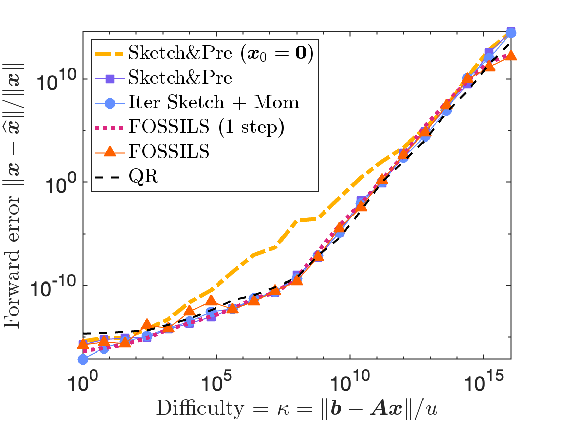
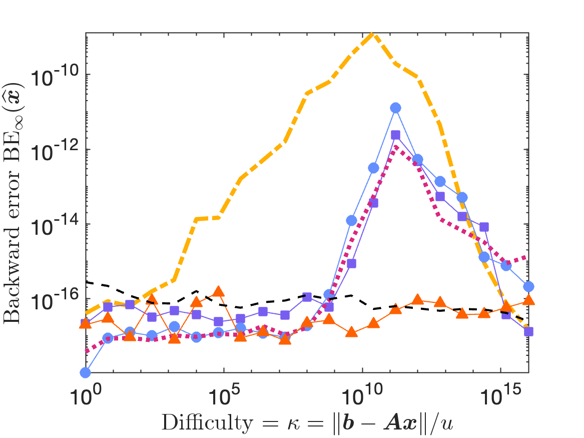
Figure 2: Forward error (left) and backward error (right) for different least-squares solvers of different difficulties 4.1. FOSSILS is the only fast backward stable randomized least-squares solver, achieving comparable backward error to Householder QR.

We test stable and unstable versions of sketch-and-precondition, iterative sketching with momentum, FOSSILS, and (Householder) QR. For sketch-and-precondition, we set $d\coloneqq 20n$ and run for $100$ iterations. For iterative sketching with momentum, we use the implementation recommended in [Epp24, sec. 3.3 and app. B]. For FOSSILS, we use Algorithm 7.

Figure 2 shows the forward (left) and backward (right) errors for these solvers on a sequence of randomly generated least-squares problems with varying difficulties. The major finding is the confirmation of backward stability of FOSSILS for problems of all difficulties, achieving comparable backward error to QR for all problems. We note in particular that, for highly ill-conditioned problems $\kappa\gtrapprox 10^{14}$, the regularization approach developed in section 3.4 yields a convergent and backward stable scheme.

To see that two refinement steps with the FOSSILS outer solver are necessary, Fig. 2 also shows the forward and backward error for the output $\boldsymbol{x}_{1}$ of a single call to the FOSSILS outer solver, listed in the figure as FOSSILS (1 step). We run FOSSILS (1 step) for 100 iterations to ensure convergence. Even with 100 iterations, FOSSILS (1 step) shows similar stability properties to iterative sketching and sketch-and-precondition, being forward but not backward stable. This demonstrates that both refinement steps in FOSSILS are necessary to obtain a backward stable scheme.

Figure 2 contains other interesting findings. The forward error curves for the forward and backward stable methods shows a kink roughly at $\mathrm{difficulty}=u^{-1/2}$, indicating a transition from the forward error being dominated by the first and second terms in Wedin’s theorem (Fact 2.4). Sketch-and-precondition with the zero initialization is unstable, but the forward error becomes comparable to that of the stable methods when the difficulty is roughly $\mathrm{difficulty}=u^{-3/4}$. Finally, we note that the forward stable methods (iterative sketching with momentum and stable sketch-and-precondition) are backward stable for problem difficulties up to $\approx u^{-1/2}$, after which the backward error climbs for difficulties up to $\approx u^{-3/4}$ before falling afterwards. These methods have acceptable stability properties for many use cases. However, since FOSSILS converges just as rapidly as these methods, we believe FOSSILS is the appropriate solver whenever a fully backward stable solution is demanded.

We further confirm the backward stability of FOSSILS in Fig. 3, where we show a contour plot of the backward error for FOSSILS (left) and iterative sketching with momentum (right) for combinations of parameters $\kappa,\left\|\boldsymbol{b}-\boldsymbol{A}\boldsymbol{x}\right\|/u\in[1,10^{16}]$. As we see in the left panel, the backward error for FOSSILS is always small multiple of machine precision, regardless of the conditioning of $\boldsymbol{A}$ or the residual norm $\|\boldsymbol{b}-\boldsymbol{A}\boldsymbol{x}\|$.

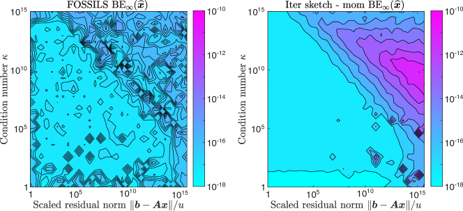
Figure 3: The backward error for FOSSILS (left) and iterative sketching with momentum (right) for sequences of randomly generated least-squares problems (generated as in Fig. 1) varying condition number $\kappa$ and scaled residual norm $\|\boldsymbol{b}-\boldsymbol{A}\boldsymbol{x}\|/u$. We set the embedding dimension $d\coloneqq 12n$ and the backward error tolerance parameter to $4\left\|\boldsymbol{A}\right\|_{\rm F}u$.

4.2 Runtime and iteration count

In this section, we present a runtime comparison of FOSSILS to MATLAB’s QR-based direct solver mldivide and iterative sketching with momentum.

For our first experiments, we test on dense least-squares problems from applications:

• Kernel regression for exotic particle detection. We consider least-squares problems for fitting the SUSY dataset [BSW14] using a linear combination of kernel functions. We adopt the same setup as in [Epp24, sec. 3.4], yielding real-valued least-squares problems of dimension $m=10^{6}$ and $n\in[10^{1},10^{3}]$. The condition numbers of these problems range from $\approx 10^{1}$ (for $n=10^{1}$) to $\approx 10^{7}$ (for $n=10^{3}$) and the residual is large $\left\|\boldsymbol{b}-\boldsymbol{A}\boldsymbol{x}\right\|/\left\|\boldsymbol{b}\right\|\approx 0.5$.

• Prony’s method and quantum eigenvalue algorithms. We consider a family of least-squares problems of dimension $m=7.5\times 10^{5}$ and $n\in[10^{1},10^{3}]$ that arise from applying Prony’s method to estimate eigenvalues from noisy measurements from a quantum device. See appendix B for details. The resulting least-squares problems are complex-valued $\boldsymbol{A}\in\mathbb{C}^{m\times n},\boldsymbol{b}\in\mathbb{C}^{m}$ with a condition number of $\approx 10^{6}$ and residual of $\left\|\boldsymbol{b}-\boldsymbol{A}\boldsymbol{x}\right\|/\left\|\boldsymbol{b}\right\|\approx 10^{-6}$.

Results are shown in Fig. 4. For both FOSSILS and iterative sketching with momentum, we use embedding dimension $d\coloneqq 12n$. We find that FOSSILS is faster than mldivide for both problems at roughly $n\approx 50$, achieving a maximal speedup of 14$\times$ (kernel regression) and 11$\times$ (Prony) at $n=10^{3}$. In particular, we note that the speed of FOSSILS is comparable to iterative sketching with momentum. With our recommended implementation, the backward stable FOSSILS solver is essentially just as fast as the forward stable iterative sketching with momentum method.

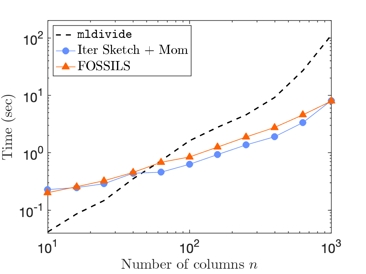
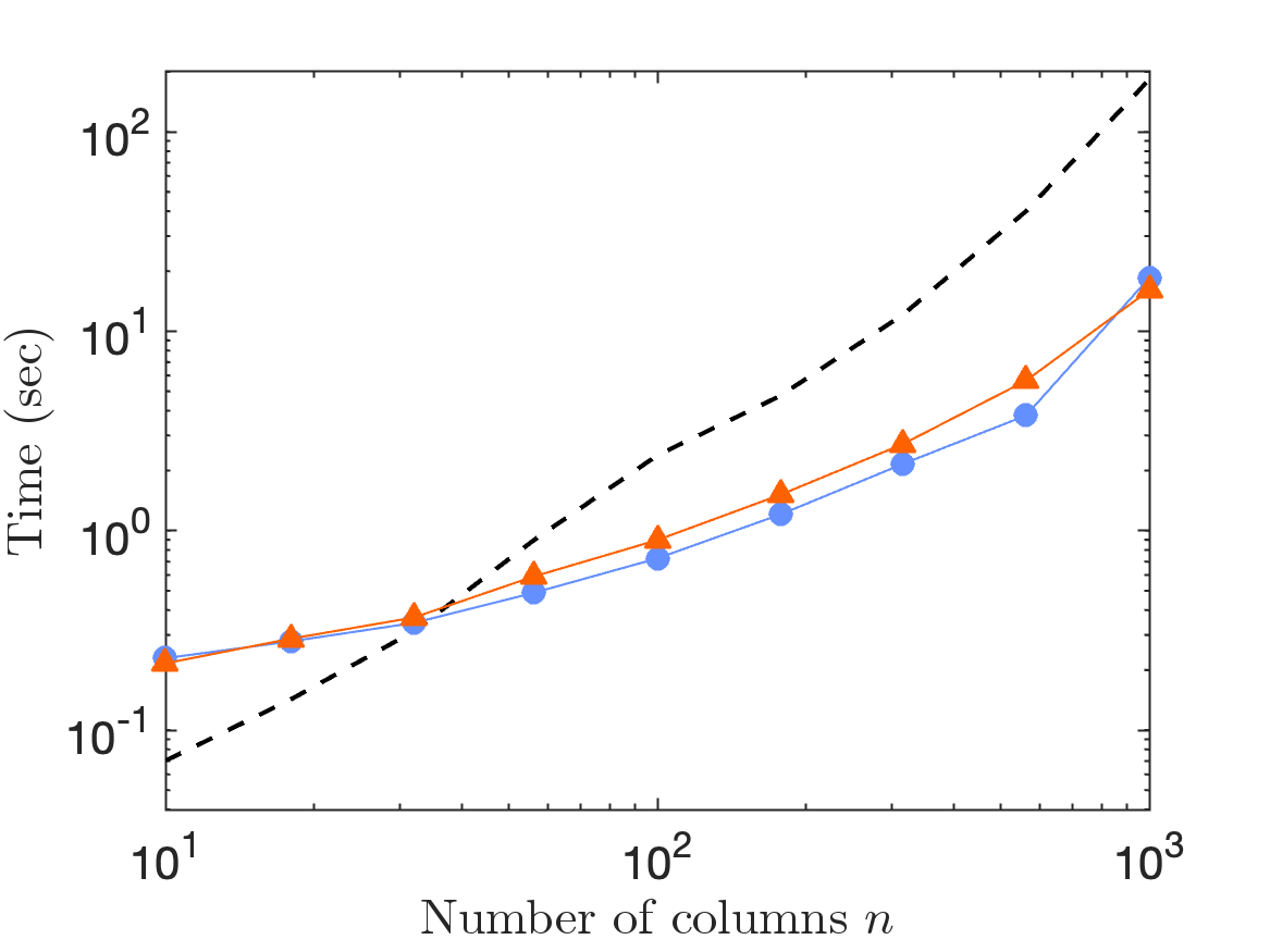
Figure 4: Runtime of FOSSILS, iterative sketching with momentum, and MATLAB’s QR-based mldivide solver for kernel regression (real-valued, left) and Prony (complex-valued, right) dense least-squares problems.

As a second timing experiment, we test FOSSILS and mldivide on problems for the SuiteSparse Matrix Collection [DH11]. We consider all rectangular problems in the collection with at least $m=10^{5}$ rows and $n=10^{2}$ columns, transposing wide matrices so that they are tall. We remove any matrices that are structurally rank-deficient and consider the first ten problems, sorted by $n$. For each matrix, we generate $\boldsymbol{b}$ to have independent standard normal entries. Timings for mldivide and FOSSILS are shown in Table 2. As these results show, the runtime of mldivide depends sensitively on the sparsity pattern. Problems 5–9 possess a low fill-in QR factorization and mldivide is 20$\times$ to a 1000$\times$ faster than FOSSILS. However, FOSSILS is 2.5$\times$ to 39$\times$ faster than mldivide on problems 1–4 and 10, which lack a benevolent sparsity pattern. We note that the stability of randomized iterative methods for sparse matrices is poorly understood; for matrices with few nonzero entries, sketch-and-precondition has been observed to be stable even with the zero initialization.

Table 2: Runtime for FOSSILS and MATLAB’s mldivide for ten problems from the SuiteSparse Matrix Collection [DH11]. Here, nnz reports the number of nonzero entries in the matrix and speedup reports the ratio of the mldivide and FOSSILS runtimes. For problems with a beneficial sparsity pattern (problems 5–9), mldivide is significantly faster than FOSSILS; for other problems, FOSSILS is faster by $2.5\times$ to $39\times$.

#	Matrix	$m$	$n$	nnz	FOSSILS	mldivide	Speedup
1	JGD_BIBD/bibd_20_10	1.8e5	1.9e2	8.3e6	0.44	1.1	2.5$\times$
2	JGD_BIBD/bibd_22_8	3.2e5	2.3e1	9.0e6	0.54	1.4	2.6$\times$
3	Mittelmann/rail2586	9.2e5	2.6e3	8.0e6	4.3	25	5.8$\times$
4	Mittelmann/rail4284	1.1e6	4.3e3	1.1e7	14	180	13$\times$
5	LPnetlib/lp_osa_30	1.0e5	4.4e3	6.0e5	14	0.13	0.010$\times$
6	Meszaros/stat96v1	2.0e5	6.0e3	5.9e5	34	0.04	0.001$\times$
7	Dattorro/EternityII_A	1.5e5	7.4e3	7.8e5	59	1.3	0.022$\times$
8	Yoshiyasu/mesh_deform	2.3e5	9.4e3	8.5e5	120	0.19	0.002$\times$
9	Dattorro/EternityII_Etilde	2.0e5	1.0e4	1.1e6	150	7.4	0.050$\times$
10	Mittelmann/spal_004	3.2e5	1.0e4	4.6e7	160	6300	39$\times$

Finally, Fig. 5 shows the number of iterations required by FOSSILS for different parameters and problem sizes. For these experiments, we use a slightly higher tolerance of $4\left\|\boldsymbol{A}\right\|_{\rm F}u$ for the backward error topping criteria. Note that these experiments correspond to the backward errors in the left panel of Fig. 3, and thus FOSSILS still achieves backward stability throughout. This figure reports two different parameter studies. In the left panel, Fig. 5 shows the number of iterations for different values of the condition number $\kappa$ and residual norm $\|\boldsymbol{b}-\boldsymbol{A}\boldsymbol{x}\|$ for randomly generated problems of size $4000\times 50$. For these problems, the number of iterations tends to be smaller for problems large $\kappa$ or small $\left\|\boldsymbol{b}-\boldsymbol{A}\boldsymbol{x}\right\|$. In all cases, however, the number of iterations is at most 45. In the right panel, Fig. 5 shows number of iterations for randomly generated problems of different sizes $10^{3}\leq m\leq 10^{6}$ and $50\leq n\leq 10^{4}$, while fixing $\kappa=10^{8}$ and $\left\|\boldsymbol{b}-\boldsymbol{A}\boldsymbol{x}\right\|=10^{-3}$. We observe that the iteration count remains consistent across these $m,n$ values.

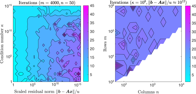
Figure 5: The number of iterations until FOSSILS reaches convergence for different values of $\kappa,\left\|\boldsymbol{b}-\boldsymbol{A}\boldsymbol{x}\right\|$, as in Fig. 3 (left) and for different values of $m\geq n$ (right). We set $d\coloneqq 12n$ for all experiments and use the backward error tolerance $4\left\|\boldsymbol{A}\right\|_{\rm F}u$.

5 FOSSILS: Stability analysis

In this section, we provide an analysis of the FOSSILS method in finite-precision arithmetic. Our main result is as follows:

Theorem 5.1 (FOSSILS: backward stability).

Assume the following:

1. Numerically full-rank. The condition number $\kappa$ satisfies $\kappa u\ll 1$ (see formal definition below).

2. Non-pathological rounding errors. The output satisfies the non-pathological rounding error assumption, defined below in section 5.1.

3. Stable sketching. The matrix $\boldsymbol{S}$ is sketching matrix for $\boldsymbol{A}$ with $d\leq n^{3}$ rows, distortion $\eta\leq 0.9$, and a forward stable multiply operation

   $$\left\|\operatorname{fl}(\boldsymbol{S}\boldsymbol{A})-\boldsymbol{S}\boldsymbol{A}\right\|\lesssim\left\|\boldsymbol{A}\right\|u.$$ (5.1)

4. Parameters for Polyak solver. Set $\alpha$ and $\beta$ according to a distortion $1.01\eta$, i.e.,

   $$\alpha=(1-(1.01\eta)^{2})^{2},\quad\beta=(1.01\eta)^{2}$$ (5.2)

   and assume $|\widehat{\alpha}-\alpha|,|\widehat{\beta}-\beta|\lesssim u$. Set the iteration count

   $$q\geq q_{0}\coloneqq\max\left(1+2\frac{\log(1/(\kappa u))}{\log(1/(1.01\eta))},11\right).$$ (5.3)

Then FOSSILS is backward stable. In particular, choosing $\boldsymbol{S}$ to be a sparse sign embedding with distortion $\eta=1/2$ with the parameter settings 2.2, FOSSILS produces a backward stable solution in $\mathcal{O}(mn\log(n/u)+n^{3}\log n)$ operations.

The rest of this section will present a proof of this result. We will then discuss how this analysis extends to a broader class of algorithms in section 6. To simplify the presentation, we introduce some notation and assumptions which we globally enforce throughout this section:

Notation and assumptions.

We remind the reader that the relation $\alpha\lesssim\beta$ indicates that $\alpha\leq C(m,n)\beta$, where $C(m,n)$ is a polynomial function in the $m$ and $n$. We will write $\alpha\ll\beta$ to indicate that $\alpha\ll\beta/C(m,n)$ for some sufficiently large polynomial function $C(m,n)$. Vectors $\boldsymbol{e}$, $\boldsymbol{e}^{\prime}$, $\boldsymbol{e}_{1}$ $\boldsymbol{e}_{2}$, $\boldsymbol{e}_{1,2}$, etc. denote arbitrary vectors of norm $\lesssim u$. We emphasize that we make no attempts to compute or optimize the value of the constants in our proofs; as our numerical experiments demonstrate, FOSSILS appears to be have similar backward and forward error to QR in practice.

The numerically computed version of a quantity $\boldsymbol{f}$ is denoted by $\operatorname{fl}(\boldsymbol{f})$ or $\boldsymbol{\widehat{f}}$ and the error is $\operatorname{err}(\boldsymbol{f})\coloneqq\boldsymbol{\widehat{f}}-\boldsymbol{f}$. A vector is exactly represented if $\operatorname{fl}(\boldsymbol{f})=\boldsymbol{f}$. We assume throughout that quantities are evaluated in the sensible way, e.g., $\boldsymbol{A}\boldsymbol{R}^{-1}\boldsymbol{z}$ is evaluated as $\boldsymbol{A}(\boldsymbol{R}^{-1}\boldsymbol{z})$. All triangular solves, e.g., $\boldsymbol{R}^{-1}\boldsymbol{z}$, are computed by back substitution.

By homogeneity, we are free to normalize the least-squares problem 1.1 so that

$$\left\|\boldsymbol{A}\right\|=\left\|\boldsymbol{b}\right\|=1.$$ (5.4)

We use this normalization throughout this section. The condition number is $\kappa\coloneqq\sigma_{\rm max}(\boldsymbol{A})/\sigma_{\rm min}(\boldsymbol{A})$. We assume throughout this section that $\kappa u\ll 1$.

5.1 The non-pathological rounding error assumption

Wedin’s theorem (Fact 2.4) tells us that a backward stable solution $\boldsymbol{\widehat{x}}$ obeys the forward error bound

$$\left\|\boldsymbol{\widehat{x}}-\boldsymbol{x}\right\|\lesssim\kappa(\left\|\boldsymbol{x}\right\|+\kappa\left\|\boldsymbol{b}-\boldsymbol{A}\boldsymbol{x}\right\|)u.$$

If the magnitude of the rounding errors agrees with Wedin’s theorem and the errors are assumed generic (i.e., random), then we would expect the norm of the computed solution to have size

$$\left\|\boldsymbol{\widehat{x}}\right\|\gtrsim\left\|\boldsymbol{x}\right\|+\kappa(\left\|\boldsymbol{x}\right\|+\kappa\left\|\boldsymbol{b}-\boldsymbol{A}\boldsymbol{x}\right\|)u.$$ (5.5)

We call 5.5 the non-pathological rounding error assumption.

We believe the non-pathological rounding error assumption essentially always holds for the output of FOSSILS. In ordinary floating point arithmetic, rounding errors are not random [Hig02, sec. 1.17], but they often behave as if they are [HM19]. If the non-pathological rounding error assumption were to not hold, the rounding errors would have to occur in a very particular way to lead to a numerical solution of very small norm. We have never seen a violation of the non-pathological rounding error assumption in our numerical experiments. Finally, we note that we have posterior estimates for the backward error (section 3.3), so a small backward error for the computed solution can always be certified at runtime at small cost.

Finally, we note one case where the non-pathological rounding error is always true:

Proposition 5.2 (Non-pathological rounding errors).

The non-pathological rounding error assumption 5.5 holds provided that the true solution $\boldsymbol{x}$ satisfies $\left\|\boldsymbol{x}\right\|\gg\kappa(\left\|\boldsymbol{x}\right\|+\kappa\left\|\boldsymbol{b}-\boldsymbol{A}\boldsymbol{x}\right\|)u$.

This result tells us that the non-pathological rounding error assumption could fail only on problems where the relative forward error of the computed solution could be high $\left\|\boldsymbol{\widehat{x}}-\boldsymbol{x}\right\|/\left\|\boldsymbol{x}\right\|\gtrsim 1$.

5.2 Stability of sketching

In this section, we prove an analog of the “whitening result” Fact 2.3 in finite precision arithmetic.

Lemma 5.3 (Stability of sketching).

Assume the hypotheses of Theorem 5.1 and let $\smash{\boldsymbol{\widehat{R}}}$ be the computed R-factor of QR decomposition of $\boldsymbol{S}\boldsymbol{A}$ computed using Householder QR. Then

$$\left\|\smash{\boldsymbol{\widehat{R}}}^{-1}\right\| \leq 20\kappa, \left\|\smash{\boldsymbol{\widehat{R}}}\right\| \leq 2,$$ (5.6)

$$\frac{1}{1+\eta}-\sigma_{\rm min}(\boldsymbol{A}\smash{\boldsymbol{\widehat{R}}}^{-1}) \lesssim\kappa u, \left\|\smash{\boldsymbol{A}\smash{\boldsymbol{\widehat{R}}}^{-1}}\right\|-\frac{1}{1-\eta} \lesssim\kappa u.$$ (5.7)

Proof.

By assumption 5.1 and the normalization $\left\|\boldsymbol{A}\right\|=1$, we have

$$\left\|\operatorname{fl}(\boldsymbol{S}\boldsymbol{A})-\boldsymbol{S}\boldsymbol{A}\right\|\lesssim u.$$

Thus, by this bound and the backward stability of Householder QR factorization [Hig02, Thm. 19.4], there exists a perturbation $\boldsymbol{E}$ of size $\left\|\boldsymbol{E}\right\|\lesssim u$ and a matrix $\boldsymbol{\widetilde{Q}}$ with orthonormal columns such that

$$\boldsymbol{S}\boldsymbol{A}+\boldsymbol{E}=\boldsymbol{\widetilde{Q}}\boldsymbol{\widehat{R}}.$$ (5.8)

We begin by proving 5.6. Throughout, let $\boldsymbol{QR}=\boldsymbol{SA}$ be the exact QR decomposition of $\boldsymbol{SA}$. Applying Weyl’s inequality [Ste98, Sec. 4.3] to 5.8, we obtain

$$\sigma_{\rm min}(\boldsymbol{\widehat{R}})=\sigma_{\rm min}(\boldsymbol{\widetilde{Q}}\boldsymbol{\widehat{R}})\geq\sigma_{\rm min}(\boldsymbol{S}\boldsymbol{A})-\left\|\boldsymbol{E}\right\|=\sigma_{\rm min}(\boldsymbol{R})-\left\|\boldsymbol{E}\right\|\geq\frac{1-\eta}{\kappa}-\left\|\boldsymbol{E}\right\|\geq\frac{1}{20\kappa}.$$

In the penultimate inequality, we use the fact that $\sigma_{\rm min}(\boldsymbol{A})=1/\kappa$ and 2.6. In the final inequality, we use the fact that $\eta\leq 0.9$ and use the standing assumption $\kappa u\ll 1$ to enforce $\left\|\boldsymbol{E}\right\|\leq(20\kappa)^{-1}$. The first inequality of 5.6 is proven. To obtain the second inequality, we take norms of 5.8:

$$\left\|\smash{\boldsymbol{\widehat{R}}}\right\|=\left\|\smash{\boldsymbol{\widetilde{Q}}\smash{\boldsymbol{\widehat{R}}}}\right\|\leq\left\|\boldsymbol{S}\boldsymbol{A}\right\|+\left\|\boldsymbol{E}\right\|=\left\|\boldsymbol{R}\right\|+\left\|\boldsymbol{E}\right\|\leq(1+\eta)+\left\|\boldsymbol{E}\right\|\leq 2.$$

The penultimate inequality is 2.6. In the final inequality, we use the assumption $\eta\leq 0.9$ and the standing assumption $u\ll 1$ to enforce $\left\|\boldsymbol{E}\right\|\leq 0.1$. This completes the proof of 5.6.

Now we prove 5.7. By the embedding property and 5.8, we have

$$\begin{split}\left\|\boldsymbol{A}\smash{\boldsymbol{\widehat{R}}}^{-1}\right\|&=\max_{\left\|\boldsymbol{u}\right\|=1}\left\|\boldsymbol{A}\smash{\boldsymbol{\widehat{R}}}^{-1}\boldsymbol{u}\right\|\leq\frac{1}{1-\eta}\cdot\max_{\left\|\boldsymbol{u}\right\|=1}\left\|\boldsymbol{S}\boldsymbol{A}\smash{\boldsymbol{\widehat{R}}}^{-1}\boldsymbol{u}\right\|\\ &=\frac{1}{1-\eta}\cdot\left\|\smash{\boldsymbol{\widetilde{Q}}-\boldsymbol{E}\smash{\boldsymbol{\widehat{R}}}^{-1}}\right\|\leq\frac{1}{1-\eta}+400\kappa\left\|\boldsymbol{E}\right\|.\end{split}$$

In the last inequality, we use the triangle inequality and 5.6. Rearranging gives the second inequality of 5.7. The proof of the first inequality of 5.7 is similar and is omitted. ∎

5.3 Basic stability results

We begin by presenting some standard results from rounding error analysis, making using of our “$\boldsymbol{e}$ notation”. The first concern stability for addition and multiplication [Hig02, secs. 2–3]:

Fact 5.4 (Basic stability results).

For exactly representable vectors $\boldsymbol{w}$ and $\boldsymbol{z}$ in ^m or ⁿ and exactly representable $\gamma\in$, we have

$$\left\|\operatorname{err}(\boldsymbol{z}\pm\boldsymbol{w})\right\|\lesssim\left\|\boldsymbol{z}\pm\boldsymbol{w}\right\|u,\quad\left\|\operatorname{err}(\gamma\cdot\boldsymbol{z})\right\|\lesssim|\gamma|\left\|\boldsymbol{z}\right\|u.$$

For matrix multiplication by $\boldsymbol{A}$ normalized as in 5.4, we have

$$\left\|\operatorname{err}(\boldsymbol{A}\boldsymbol{z})\right\|\lesssim\left\|\boldsymbol{z}\right\|u,\quad\left\|\operatorname{err}(\boldsymbol{A}^{\top}\boldsymbol{z})\right\|\lesssim\left\|\boldsymbol{z}\right\|u.$$

We also have the following characterization of the backward stability of triangular solves.

Proposition 5.5 (Backward stability of triangular solves).

Instate the asssumptions of Theorem 5.1 and let $\boldsymbol{z}\in^{n}$ be exactly representable. Then

$$\operatorname{err}(\smash{\boldsymbol{\widehat{R}}}^{-1}\boldsymbol{z})=\left\|\smash{\boldsymbol{\widehat{R}}}^{-1}\boldsymbol{z}\right\|\cdot\smash{\boldsymbol{\widehat{R}}}^{-1}\boldsymbol{e},\quad\operatorname{err}(\smash{\boldsymbol{\widehat{R}}}^{-\top}\boldsymbol{z})=\left\|\smash{\smash{\boldsymbol{\widehat{R}}}^{-\top}\boldsymbol{z}}\right\|\cdot\smash{\boldsymbol{\widehat{R}}}^{-\top}\boldsymbol{e}^{\prime}.$$

Proof.

The classical statement of the backward stability of triangular solves [Hig02, sec. 8.1] is that there exist a perturbation $\boldsymbol{\Delta R}$ such that

$$(\smash{\boldsymbol{\widehat{R}}}+\boldsymbol{\Delta R})(\smash{\boldsymbol{\widehat{R}}}^{-1}\boldsymbol{z}+\operatorname{err}(\smash{\boldsymbol{\widehat{R}}}^{-1}\boldsymbol{z}))=\boldsymbol{z},\quad\left\|\boldsymbol{\Delta R}\right\|\lesssim\left\|\smash{\boldsymbol{\widehat{R}}}\right\|u.$$

Subtracting $\boldsymbol{z}+\boldsymbol{\Delta R}\cdot\smash{\boldsymbol{\widehat{R}}}^{-1}\boldsymbol{z}$ from both sides yields

$$(\smash{\boldsymbol{\widehat{R}}}+\boldsymbol{\Delta R})\operatorname{err}(\smash{\boldsymbol{\widehat{R}}}^{-1}\boldsymbol{z})=-\boldsymbol{\Delta R}\cdot\smash{\boldsymbol{\widehat{R}}}^{-1}\boldsymbol{z}.$$

Multiplying by $(\smash{\boldsymbol{\widehat{R}}}+\boldsymbol{\Delta R})^{-1}=\smash{\boldsymbol{\widehat{R}}}^{-1}(\mathbf{I}+\boldsymbol{\Delta R}\cdot\smash{\boldsymbol{\widehat{R}}}^{-1})^{-1}$ yields

$$\operatorname{err}(\smash{\boldsymbol{\widehat{R}}}^{-1}\boldsymbol{z})=\smash{\boldsymbol{\widehat{R}}}^{-1}(\mathbf{I}+\boldsymbol{\Delta R}\cdot\smash{\boldsymbol{\widehat{R}}}^{-1})^{-1}\left(-\boldsymbol{\Delta R}\cdot\smash{\boldsymbol{\widehat{R}}}^{-1}\boldsymbol{z}\right).$$

The matrix $\mathbf{I}+\smash{\boldsymbol{\widehat{R}}}^{-1}\cdot\boldsymbol{\Delta R}$ is invertible because $\left\|\boldsymbol{\Delta R}\cdot\smash{\boldsymbol{\widehat{R}}}^{-1}\right\|\lesssim\kappa u\ll 1$ by Lemma 5.3. Thus, we are free to assume $\left\|\smash{\boldsymbol{\widehat{R}}}^{-1}\cdot\boldsymbol{\Delta R}\right\|\leq 1/2$ and thus $\left\|(\mathbf{I}+\smash{\boldsymbol{\widehat{R}}}^{-1}\cdot\boldsymbol{\Delta R})^{-1}\right\|\leq 2$. Therefore,

$$\left\|(\mathbf{I}+\boldsymbol{\Delta R}\cdot\smash{\boldsymbol{\widehat{R}}}^{-1})^{-1}\left(-\boldsymbol{\Delta R}\cdot\smash{\boldsymbol{\widehat{R}}}^{-1}\boldsymbol{z}\right)\right\|\leq 2\left\|\boldsymbol{\Delta R}\right\|\left\|\smash{\boldsymbol{\widehat{R}}}^{-1}\boldsymbol{z}\right\|\lesssim\left\|\smash{\boldsymbol{\widehat{R}}}^{-1}\boldsymbol{z}\right\|u.$$

Here, we used the bound 5.6. Finally, use the bound $\left\|\boldsymbol{z}\right\|\leq\left\|\smash{\boldsymbol{\widehat{R}}}\right\|\left\|\smash{\boldsymbol{\widehat{R}}}^{-1}\boldsymbol{z}\right\|\lesssim\left\|\smash{\boldsymbol{\widehat{R}}}^{-1}\boldsymbol{z}\right\|$ to reach the stated result for $\operatorname{err}(\smash{\boldsymbol{\widehat{R}}}^{-1}\boldsymbol{z})$. The result for $\operatorname{err}(\smash{\boldsymbol{\widehat{R}}}^{-\top}\boldsymbol{z})$ is proven in the same way. ∎

By combining Facts 5.4 and 5.5, we can analyze the effect of multiplying by $\boldsymbol{A}\smash{\boldsymbol{\widehat{R}}}^{-1}$ and variations thereof:

Proposition 5.6 (Multiplication by whitened basis).

Instate the asssumptions of Theorem 5.1 and normalization 5.4. For an exactly representable vector $\boldsymbol{z}$ of the appropriate size,

$$\operatorname{err}(\smash{\boldsymbol{\widehat{R}}}^{-\top}\boldsymbol{A}^{\top}\boldsymbol{z}) =\left\|\boldsymbol{z}\right\|\cdot\smash{\boldsymbol{\widehat{R}}}^{-\top}\boldsymbol{e},$$ (5.9)

$$\left\|\operatorname{err}(\smash{\boldsymbol{\widehat{R}}}^{-\top}\boldsymbol{A}^{\top}\boldsymbol{A}\smash{\boldsymbol{\widehat{R}}}^{-1}\boldsymbol{z})\right\| \lesssim\kappa u\left\|\boldsymbol{z}\right\|.$$ (5.10)

Proof.

We begin by proving 5.9. By Fact 5.4, we have

$$\operatorname{err}(\boldsymbol{A}^{\top}\boldsymbol{z})=\left\|\boldsymbol{z}\right\|\cdot\boldsymbol{e}_{1}.$$

By Proposition 5.5, we obtain

$$\operatorname{err}(\smash{\boldsymbol{\widehat{R}}}^{-\top}\boldsymbol{A}^{\top}\boldsymbol{z})=\left\|\boldsymbol{z}\right\|\cdot\smash{\boldsymbol{\widehat{R}}}^{-\top}\boldsymbol{e}_{1}+\left\|\smash{\boldsymbol{\widehat{R}}}^{-\top}(\boldsymbol{A}^{\top}\boldsymbol{z}+\left\|\boldsymbol{z}\right\|\cdot\boldsymbol{e}_{1})\right\|\cdot\smash{\boldsymbol{\widehat{R}}}^{-\top}\boldsymbol{e}_{2}.$$ (5.11)

By the triangle inequality, the submultiplicative property, and Lemma 5.3, we have

$$\left\|\smash{\boldsymbol{\widehat{R}}}^{-\top}\left(\boldsymbol{A}^{\top}\boldsymbol{z}+\left\|\boldsymbol{z}\right\|\cdot\boldsymbol{e}_{1}\right)\right\|\leq\left(\left\|\boldsymbol{A}\smash{\boldsymbol{\widehat{R}}}^{-1}\right\|+\left\|\smash{\boldsymbol{\widehat{R}}}^{-\top}\boldsymbol{e}_{1}\right\|\right)\left\|\boldsymbol{z}\right\|\lesssim(1+\kappa u)\left\|\boldsymbol{z}\right\|\lesssim\left\|\boldsymbol{z}\right\|.$$

This establishes that the right-hand side of 5.11 has the form $\left\|\boldsymbol{z}\right\|\cdot\smash{\boldsymbol{\widehat{R}}}^{-\top}\boldsymbol{e}$, proving 5.9.

We now prove 5.10. By Proposition 5.5,

$$\operatorname{err}(\smash{\boldsymbol{\widehat{R}}}^{-1}\boldsymbol{z})=\left\|\smash{\boldsymbol{\widehat{R}}}^{-1}\boldsymbol{z}\right\|\cdot\smash{\boldsymbol{\widehat{R}}}^{-1}\boldsymbol{e}_{3}=\kappa\left\|\boldsymbol{z}\right\|\cdot\smash{\boldsymbol{\widehat{R}}}^{-1}\boldsymbol{e}_{4}.$$

In the second equality, we used the fact that $\left\|\smash{\smash{\boldsymbol{\widehat{R}}}^{-1}\boldsymbol{z}}\right\|\lesssim\kappa\left\|\boldsymbol{z}\right\|$ by Lemma 5.3. By Fact 5.4, we have

$$\operatorname{err}(\boldsymbol{A}\smash{\boldsymbol{\widehat{R}}}^{-1}\boldsymbol{z})=\kappa\left\|\boldsymbol{z}\right\|\cdot\boldsymbol{A}\smash{\boldsymbol{\widehat{R}}}^{-1}\boldsymbol{e}_{4}+\left\|\smash{\boldsymbol{\widehat{R}}}^{-1}(\boldsymbol{z}+\kappa\left\|\boldsymbol{z}\right\|\cdot\boldsymbol{e}_{4})\right\|\cdot\boldsymbol{e}_{5}.$$

By Lemma 5.3, we have $\left\|\boldsymbol{A}\smash{\boldsymbol{\widehat{R}}}^{-1}\boldsymbol{e}_{4}\right\|\lesssim u$ and

$$\left\|\smash{\boldsymbol{\widehat{R}}}^{-1}(\boldsymbol{z}+\kappa\left\|\boldsymbol{z}\right\|\cdot\boldsymbol{e}_{4})\right\|\leq\sigma_{\rm min}(\smash{\boldsymbol{\widehat{R}}})^{-1}(1+\kappa\left\|\boldsymbol{e}_{4}\right\|)\left\|\boldsymbol{z}\right\|\lesssim\kappa\left\|\boldsymbol{z}\right\|.$$

Here, we used the assumption that $\kappa\left\|\boldsymbol{e}_{4}\right\|\lesssim\kappa u\lesssim 1$. Thus, we have shown $\left\|\operatorname{err}(\boldsymbol{A}\smash{\boldsymbol{\widehat{R}}}^{-1}\boldsymbol{z})\right\|\lesssim\kappa u\left\|\boldsymbol{z}\right\|$. Combining with 5.9, we obtain

$$\left\|\operatorname{err}(\smash{\boldsymbol{\widehat{R}}}^{-\top}\boldsymbol{A}^{\top}\boldsymbol{A}\smash{\boldsymbol{\widehat{R}}}^{-1}\boldsymbol{z})\right\|=\left\|\left\|\boldsymbol{A}\smash{\boldsymbol{\widehat{R}}}^{-1}\boldsymbol{z}+\operatorname{err}(\boldsymbol{A}\smash{\boldsymbol{\widehat{R}}}^{-1}\boldsymbol{z})\right\|\cdot\smash{\boldsymbol{\widehat{R}}}^{-\top}\boldsymbol{e}_{6}+\smash{\boldsymbol{\widehat{R}}}^{-\top}\boldsymbol{A}^{\top}\operatorname{err}(\boldsymbol{A}\smash{\boldsymbol{\widehat{R}}}^{-1}\boldsymbol{z})\right\|$$

$$\qquad\leq(\left\|\boldsymbol{A}\smash{\boldsymbol{\widehat{R}}}^{-1}\right\|\left\|\boldsymbol{z}\right\|+\left\|\operatorname{err}(\boldsymbol{A}\smash{\boldsymbol{\widehat{R}}}^{-1}\boldsymbol{z})\right\|)\left\|\smash{\smash{\boldsymbol{\widehat{R}}}^{-\top}}\right\|\left\|\boldsymbol{e}_{6}\right\|+\left\|\smash{\boldsymbol{\widehat{R}}}^{-\top}\boldsymbol{A}^{\top}\right\|\left\|\operatorname{err}(\boldsymbol{A}\smash{\boldsymbol{\widehat{R}}}^{-1}\boldsymbol{z})\right\|\lesssim\kappa u\left\|\boldsymbol{z}\right\|.$$

The final inequality uses Lemma 5.3 and the bound $\left\|\operatorname{err}(\boldsymbol{A}\smash{\boldsymbol{\widehat{R}}}^{-1}\boldsymbol{z})\right\|\lesssim\kappa u\left\|\boldsymbol{z}\right\|$. ∎

5.4 Stability of Polyak heavy ball iteration

We have the following guaratee for the Polyak solver in finite precision:

Lemma 5.7 (Stability of Polyak heavy ball).

Instate the assumptions of Theorem 5.1. Then the output of Algorithm 2 satisfies

$$\left\|\operatorname{fl}(\textsc{Polyak}(\boldsymbol{c}))-(\smash{\boldsymbol{\widehat{R}}}^{-\top}\boldsymbol{A}^{\top}\boldsymbol{A}\smash{\boldsymbol{\widehat{R}}}^{-1})^{-1}\boldsymbol{c}\right\|\lesssim\kappa u\cdot\left\|\boldsymbol{c}\right\|.$$

Proof.

By Lemma 5.3 and the assumption $\kappa u\ll 1$, the numerically computed preconditioner satisfies 2.7 with distortion parameter $1.01\eta$. Thus, we are in the setting to apply Lemma 3.2.

The Polyak iterates $\boldsymbol{\widehat{y}}_{i}$ evaluated in floating point satisfy a recurrence

$$\boldsymbol{\widehat{y}}_{i+1}=\boldsymbol{\widehat{y}}_{i}+\alpha(\boldsymbol{c}-\smash{\boldsymbol{\widehat{R}}}^{-\top}\boldsymbol{A}^{\top}\boldsymbol{A}\smash{\boldsymbol{\widehat{R}}}^{-1}\boldsymbol{\widehat{y}}_{i})+\beta(\boldsymbol{\widehat{y}}_{i}-\boldsymbol{\widehat{y}}_{i-1})+\boldsymbol{f}_{i},$$

where $\boldsymbol{f}_{i}$ is a vector of floating point errors incurred in applying the recurrence. By Proposition 5.6,

$$\left\|\operatorname{err}(\smash{\boldsymbol{\widehat{R}}}^{-\top}\boldsymbol{A}^{\top}\boldsymbol{A}\smash{\boldsymbol{\widehat{R}}}^{-1}\boldsymbol{\widehat{y}}_{i})\right\|\lesssim\kappa u\left\|\boldsymbol{\widehat{y}}_{i}\right\|.$$

In particular, since $\kappa u\ll 1$, $\left\|\operatorname{fl}(\smash{\boldsymbol{\widehat{R}}}^{-\top}\boldsymbol{A}^{\top}\boldsymbol{A}\smash{\boldsymbol{\widehat{R}}}^{-1}\boldsymbol{\widehat{y}}_{i})\right\|\lesssim\left\|\boldsymbol{\widehat{y}}_{i}\right\|$. By several applications of Fact 5.4, we conclude

$$\left\|\boldsymbol{f}_{i}\right\|=\left\|\operatorname{err}(\boldsymbol{\widehat{y}}_{i+1})\right\|\lesssim(\kappa\left\|\boldsymbol{\widehat{y}}_{i}\right\|+\left\|\boldsymbol{c}\right\|+\left\|\boldsymbol{\widehat{y}}_{i-1}\right\|)u\lesssim\kappa u(\left\|\boldsymbol{\widehat{y}}_{i}\right\|+\left\|\boldsymbol{c}\right\|+\left\|\boldsymbol{\widehat{y}}_{i-1}\right\|).$$

More precisely, let us say that

$$\left\|\boldsymbol{f}_{i}\right\|\leq C\kappa u(\left\|\boldsymbol{\widehat{y}}_{i}\right\|+\left\|\boldsymbol{c}\right\|+\left\|\boldsymbol{\widehat{y}}_{i-1}\right\|)$$ (5.12)

for an appropriate quantity $C$ depending polynomially on $m$ and $n$.

Now, we establish the floating point errors remain bounded across iterations; specifically,

$$\left\|\boldsymbol{f}_{i}\right\|\leq 141C\kappa u\left\|\boldsymbol{c}\right\|\quad\text{for }i=1,2,\ldots.$$ (5.13)

We prove this claim by induction. For the base case $i=1$, we have

$$\left\|\boldsymbol{f}_{1}\right\|\leq C\kappa u(\left\|\boldsymbol{\widehat{y}}_{1}\right\|+\left\|\boldsymbol{c}\right\|+\left\|\boldsymbol{\widehat{y}}_{0}\right\|)=3C\kappa u<141C\kappa u.$$

Here, we used the initial conditions $\boldsymbol{\widehat{y}}_{0}=\boldsymbol{\widehat{y}}_{1}=\boldsymbol{c}$. Now suppose that 5.13 holds up to $i$. By Lemma 3.2, we have the following bound for $j\leq i+1$:

$$\left\|\boldsymbol{\widehat{y}}_{j}\right\|\leq 4\sqrt{2}\cdot j(1.01\eta)^{j-1}\left\|\boldsymbol{c}\right\|+\frac{9}{(1-1.01\eta)^{2}}\cdot\max_{1\leq j^{\prime}\leq j-1}\left\|\boldsymbol{f}_{j}\right\|+\left\|(\smash{\boldsymbol{\widehat{R}}}^{-\top}\boldsymbol{A}^{\top}\boldsymbol{A}\smash{\boldsymbol{\widehat{R}}}^{-1})^{-1}\boldsymbol{c}\right\|.$$

Using the induction hypothesis 5.13, the hypothesis $\eta\leq 0.9$, the numerical inequality $j(1.01)^{j-1}<11$ for all $j\geq 0$, and the preconditioning result $\sigma_{\rm min}(\boldsymbol{A}\smash{\boldsymbol{\widehat{R}}}^{-1})\geq(1+1.01\eta)^{-1}$, we obtain

$$\left\|\boldsymbol{\widehat{y}}_{j}\right\|\leq 44\sqrt{2}\left\|\boldsymbol{c}\right\|+1087\cdot(141C\kappa u\left\|\boldsymbol{c}\right\|)+3.7\left\|\boldsymbol{c}\right\|\leq 70\left\|\boldsymbol{c}\right\|\quad\text{for }j\leq i+1.$$

In the last bound, we used the assumption $\kappa u\ll 1$. Plugging into 5.12, we obtain

$$\left\|\boldsymbol{f}_{i+1}\right\|\leq C\kappa u((\left\|\boldsymbol{\widehat{y}}_{i+1}\right\|+\left\|\boldsymbol{c}\right\|+\left\|\boldsymbol{\widehat{y}}_{i}\right\|))\leq 141C\kappa u.$$

This completes the proof of the claim 5.13.

Finally, using 5.13 and Lemma 3.2, we obtain

$$\left\|\boldsymbol{\widehat{y}}_{q}-(\smash{\boldsymbol{\widehat{R}}}^{-\top}\boldsymbol{A}^{\top}\boldsymbol{A}\smash{\boldsymbol{\widehat{R}}}^{-1})^{-1}\boldsymbol{c}\right\|\leq 4\sqrt{2}\cdot q(1.01\eta)^{q-1}\left\|\boldsymbol{c}\right\|+141C\kappa u\left\|\boldsymbol{c}\right\|.$$ (5.14)

The function $q\mapsto q(1.01)^{q-1}$ is monotone decreasing for $q\geq 11$. There are two cases.

• Case 1. Suppose $q_{0}=11$. Then $2\log(1/(\kappa u))/\log(1/(1.01\eta))\leq 11$ so $(1.01\eta)^{5.5}\leq\kappa u$. Thus,

  $$q(1.01\eta)^{q-1}\leq q_{0}(1.01\eta)^{q_{0}-1}=11(1.01\eta)^{4.5}(1.01\eta)^{5.5}\leq 7.2\kappa u.$$

  Substituting this bound in 5.14, we obtain the desired conclusion

  $$\left\|\boldsymbol{\widehat{y}}_{q}-(\smash{\boldsymbol{\widehat{R}}}^{-\top}\boldsymbol{A}^{\top}\boldsymbol{A}\smash{\boldsymbol{\widehat{R}}}^{-1})^{-1}\boldsymbol{c}\right\|\lesssim\kappa u\left\|\boldsymbol{c}\right\|.$$ (5.15)

• Case 2. Suppose $q_{0}>11$. Then

  $$q(1.01\eta)^{q-1} \leq q_{0}(1.01\eta)^{q_{0}-1}=\left(1+2\frac{\log(1/(\kappa u))}{\log(1/(1.01\eta))}\right)(1.01\eta)^{2\log(1/(\kappa u))/\log(1/(1.01\eta))}$$

  $$=\left(1+2\frac{\log(1/(\kappa u))}{\log(1/(1.01\eta))}\right)(\kappa u)^{2}\leq\left(1+21\log(1/(\kappa u))\right)(\kappa u)^{2}\leq 2\kappa u.$$

  In the last inequality, we use the hypothesis $\kappa u\ll 1$. Substituting this bound in 5.14, we obtain the desired conclusion 5.15.

Having exhausted both cases, we conclude that 5.15 always holds, completing the proof. ∎

5.5 How do you prove backward stability?

For direct methods such as QR factorization, backward stability is typically established by directly analyzing the algorithm, interpreting each rounding error made during computation as a perturbation to the input. For iterative methods, this approach breaks down. To establish backward stability, we will use the following structural result, a corollary of Theorem 3.5:

Corollary 5.8 (Proving backward stability).

The backward error satisfies $\operatorname{BE}_{1}(\boldsymbol{\widehat{x}})\lesssim\varepsilon$ if

$$\boldsymbol{x}-\boldsymbol{\widehat{x}}=(1+\left\|\boldsymbol{\widehat{x}}\right\|)\cdot\smash{\boldsymbol{\widehat{R}}}^{-1}\boldsymbol{f}+\left\|\boldsymbol{b}-\boldsymbol{A}\boldsymbol{\widehat{x}}\right\|\cdot(\boldsymbol{A}^{\top}\boldsymbol{A})^{-1}\boldsymbol{f}^{\prime}\quad\text{for }\left\|\boldsymbol{f}\right\|,\left\|\boldsymbol{f}^{\prime}\right\|\lesssim\varepsilon.$$ (5.16)

Proof.

Let $\boldsymbol{A}=\sum_{i=1}^{n}\sigma_{i}^{\vphantom{\top}}\boldsymbol{u}_{i}^{\vphantom{\top}}\boldsymbol{v}_{i}^{\top}$ be a singular value decomposition. Multiply 5.16 by $\boldsymbol{v}_{i}^{\top}$, then use 5.7 and the identity $\boldsymbol{v}_{i}^{\top}=\sigma_{i}^{-1}\boldsymbol{u}_{i}^{\top}\boldsymbol{A}=\sigma_{i}^{-2}\boldsymbol{v}_{i}^{\top}\boldsymbol{A}^{\top}\boldsymbol{A}$. Finally, appeal to Theorem 3.5. ∎

5.6 The error formula

With Corollary 5.8 in hand, we are now ready to establish an error formula of the form 5.16 for FOSSILS. This result will immediately lead to the backward stability result Theorem 5.1:

Lemma 5.9 (Error formula).

Instate the assumptions of Theorem 5.1 and define $\boldsymbol{r}_{i}\coloneqq\boldsymbol{b}-\boldsymbol{A}\boldsymbol{\widehat{x}}_{i}$. Then we have the following error formula

$$\boldsymbol{x}-\boldsymbol{\widehat{x}}_{i+1}=\left(1+\left\|\boldsymbol{x}\right\|+\left\|\boldsymbol{\widehat{x}}_{i}\right\|+\kappa^{2}u\left\|\boldsymbol{r}_{i}\right\|+\kappa\left\|\boldsymbol{A}(\boldsymbol{x}-\boldsymbol{\widehat{x}}_{i})\right\|\right)\cdot\smash{\boldsymbol{\widehat{R}}}^{-1}\boldsymbol{e}+\left\|\boldsymbol{r}_{i}\right\|\cdot(\boldsymbol{A}^{\top}\boldsymbol{A})^{-1}\boldsymbol{e}^{\prime}.$$

Proof.

We proceed step by step through Algorithm 3. By Fact 5.4, we have

$$\operatorname{err}(\boldsymbol{b}-\boldsymbol{A}\boldsymbol{\widehat{x}}_{i})=(\left\|\boldsymbol{r}_{i}\right\|+\left\|\boldsymbol{\widehat{x}}_{i}\right\|)\boldsymbol{e}_{1}.$$

In particular, since

$$\left\|\boldsymbol{r}_{i}\right\|\leq\left\|\boldsymbol{b}\right\|+\left\|\boldsymbol{A}\right\|\left\|\boldsymbol{\widehat{x}}_{i}\right\|=1+\left\|\boldsymbol{\widehat{x}}_{i}\right\|,$$ (5.17)

the norm of the computed residual satisfies

$$\left\|\boldsymbol{\widehat{r}}_{i}\right\|\lesssim\left\|\boldsymbol{r}_{i}\right\|+(\left\|\boldsymbol{r}_{i}\right\|+\left\|\boldsymbol{\widehat{x}}_{i}\right\|)u\lesssim\left\|\boldsymbol{r}_{i}\right\|+(1+\left\|\boldsymbol{\widehat{x}}_{i}\right\|)u.$$ (5.18)

Let $\boldsymbol{c}_{i}=\smash{\boldsymbol{\widehat{R}}}^{-\top}\boldsymbol{A}^{\top}\boldsymbol{r}_{i}$. By Proposition 5.6,

$$\operatorname{err}(\boldsymbol{c}_{i})=\operatorname{err}(\smash{\boldsymbol{\widehat{R}}}^{-\top}\boldsymbol{A}^{\top}\boldsymbol{r}_{i})=(\left\|\boldsymbol{r}_{i}\right\|+\left\|\boldsymbol{x}_{i}\right\|)\cdot\smash{\boldsymbol{\widehat{R}}}^{-\top}\boldsymbol{A}^{\top}\boldsymbol{e}_{1}+\left\|\boldsymbol{\widehat{r}}_{i}\right\|\cdot\smash{\boldsymbol{\widehat{R}}}^{-\top}\boldsymbol{e}_{2}.$$

Using 5.17, 5.18 and 5.7, this result simplifies to

$$\operatorname{err}(\boldsymbol{c}_{i})=(1+\left\|\boldsymbol{\widehat{x}}_{i}\right\|)\boldsymbol{e}_{3}+[\left\|\boldsymbol{r}_{i}\right\|+(1+\left\|\boldsymbol{\widehat{x}}_{i}\right\|)u]\smash{\boldsymbol{\widehat{R}}}^{-\top}\boldsymbol{e}_{4}.$$

By 5.6, $\left\|\smash{\boldsymbol{\widehat{R}}}^{-\top}\boldsymbol{e}_{4}\right\|\lesssim\kappa u\ll 1$, so we can further consolidate

$$\operatorname{err}(\boldsymbol{c}_{i})=(1+\left\|\boldsymbol{\widehat{x}}_{i}\right\|)\boldsymbol{e}_{5}+\left\|\boldsymbol{r}_{i}\right\|\cdot\smash{\boldsymbol{\widehat{R}}}^{-\top}\boldsymbol{e}_{4}.$$ (5.19)

By Lemma 5.7, the value of

$$\boldsymbol{y}_{i}=(\smash{\boldsymbol{\widehat{R}}}^{-\top}\boldsymbol{A}^{\top}\boldsymbol{A}\smash{\boldsymbol{\widehat{R}}}^{-1})^{-1}\boldsymbol{c}_{i}=\smash{\boldsymbol{\widehat{R}}}(\boldsymbol{A}^{\top}\boldsymbol{A})^{-1}\boldsymbol{A}^{\top}\boldsymbol{r}_{i}=\smash{\boldsymbol{\widehat{R}}}(\boldsymbol{x}-\boldsymbol{\widehat{x}}_{i}).$$ (5.20)

computed by the Polyak solver satisfies

$$\left\|\boldsymbol{\widehat{y}}_{i}-(\smash{\boldsymbol{\widehat{R}}}^{-\top}\boldsymbol{A}^{\top}\boldsymbol{A}\smash{\boldsymbol{\widehat{R}}}^{-1})^{-1}\boldsymbol{\widehat{c}}_{i}\right\|\lesssim\kappa u\left\|\boldsymbol{\widehat{c}}_{i}\right\|\leq\kappa u\left\|\boldsymbol{c}_{i}\right\|+\kappa u\left\|\operatorname{err}(\boldsymbol{c}_{i})\right\|.$$

We compute the two norms in the right-hand side of this expression. First, in view of the identity $\boldsymbol{A}^{\top}\boldsymbol{r}_{i}=\boldsymbol{A}^{\top}\boldsymbol{A}(\boldsymbol{x}-\boldsymbol{\widehat{x}}_{i})$, we compute

$$\left\|\boldsymbol{c}_{i}\right\|=\left\|\smash{\boldsymbol{\widehat{R}}}^{-\top}\boldsymbol{A}^{\top}\boldsymbol{A}(\boldsymbol{x}-\boldsymbol{\widehat{x}}_{i})\right\|\lesssim\left\|\boldsymbol{A}(\boldsymbol{x}-\boldsymbol{\widehat{x}}_{i})\right\|.$$ (5.21)

The last line is 5.7. We bound $\left\|\operatorname{err}(\boldsymbol{c}_{i})\right\|$ using 5.19, the triangle inequality, and 5.6,

$$\kappa u\left\|\operatorname{err}(\boldsymbol{c}_{i})\right\|\lesssim\kappa u(1+\left\|\boldsymbol{\widehat{x}}_{i}\right\|)u+\kappa u\left\|\boldsymbol{r}_{i}\right\|\cdot\left\|\smash{\boldsymbol{\widehat{R}}}^{-\top}\boldsymbol{e}_{4}\right\|\lesssim\left[1+\left\|\boldsymbol{\widehat{x}}_{i}\right\|+\kappa^{2}u\left\|\boldsymbol{r}_{i}\right\|\right]u.$$

Combining the three previous displays, we get

$$\left\|\boldsymbol{\widehat{y}}_{i}-(\smash{\boldsymbol{\widehat{R}}}^{-\top}\boldsymbol{A}^{\top}\boldsymbol{A}\smash{\boldsymbol{\widehat{R}}}^{-1})^{-1}\boldsymbol{\widehat{c}}_{i}\right\|\lesssim\left[1+\left\|\boldsymbol{\widehat{x}}_{i}\right\|+\kappa^{2}u\left\|\boldsymbol{r}_{i}\right\|+\kappa\left\|\boldsymbol{A}(\boldsymbol{x}-\boldsymbol{x}_{i})\right\|\right]u.$$

Therefore, we have

$$\operatorname{err}(\boldsymbol{y}_{i})=\left[1+\left\|\boldsymbol{\widehat{x}}_{i}\right\|+\kappa^{2}u\left\|\boldsymbol{r}_{i}\right\|+\kappa\left\|\boldsymbol{A}(\boldsymbol{x}-\boldsymbol{\widehat{x}}_{i})\right\|\right]\boldsymbol{e}_{6}+(\smash{\boldsymbol{\widehat{R}}}^{-\top}\boldsymbol{A}^{\top}\boldsymbol{A}\smash{\boldsymbol{\widehat{R}}}^{-1})^{-1}\operatorname{err}(\boldsymbol{c}_{i}).$$

Substituting 5.19 and simplifying, we obtain

$$\operatorname{err}(\boldsymbol{y}_{i})=\left[(1+\left\|\boldsymbol{\widehat{x}}_{i}\right\|)+\kappa^{2}u\left\|\boldsymbol{r}_{i}\right\|+\kappa\left\|\boldsymbol{A}(\boldsymbol{x}-\boldsymbol{\widehat{x}}_{i})\right\|\right]\boldsymbol{e}_{7}+\left\|\boldsymbol{r}_{i}\right\|\cdot\smash{\boldsymbol{\widehat{R}}}(\boldsymbol{A}^{\top}\boldsymbol{A})^{-1}\boldsymbol{e}_{5}.$$ (5.22)

Now we treat $\smash{\boldsymbol{\widehat{R}}}^{-1}\boldsymbol{y}_{i}$. By Proposition 5.5, we have

$$\operatorname{err}(\smash{\boldsymbol{\widehat{R}}}^{-1}\boldsymbol{y}_{i})=\left\|\smash{\boldsymbol{\widehat{R}}}^{-1}\boldsymbol{\widehat{y}}_{i}\right\|\cdot\smash{\boldsymbol{\widehat{R}}}^{-1}\boldsymbol{e}_{8}+\smash{\boldsymbol{\widehat{R}}}^{-1}\operatorname{err}(\boldsymbol{\widehat{y}}_{i}).$$

Using 5.20 and 5.19, we may bound $\left\|\smash{\boldsymbol{\widehat{R}}}^{-1}\boldsymbol{\widehat{y}}_{i}\right\|$ as

$$\left\|\smash{\boldsymbol{\widehat{R}}}^{-1}\boldsymbol{\widehat{y}}_{i}\right\| \leq\left\|\smash{\boldsymbol{\widehat{R}}}^{-1}\boldsymbol{y}_{i}\right\|+\left\|\smash{\boldsymbol{\widehat{R}}}^{-1}\operatorname{err}(\boldsymbol{y}_{i})\right\|\lesssim\left\|\boldsymbol{x}-\boldsymbol{\widehat{x}}_{i}\right\|+\left[1+\left\|\boldsymbol{\widehat{x}}_{i}\right\|+\kappa\left\|\boldsymbol{A}(\boldsymbol{x}-\boldsymbol{x}_{i})\right\|\right]u+\kappa^{2}u\left\|\boldsymbol{r}_{i}\right\|$$

$$\lesssim\left\|\boldsymbol{x}\right\|+\left\|\boldsymbol{\widehat{x}}\right\|+\left[1+\kappa\left\|\boldsymbol{A}(\boldsymbol{x}-\boldsymbol{x}_{i})\right\|+\kappa^{2}\left\|\boldsymbol{r}_{i}\right\|\right]u$$

Combining the two previous displays and 5.22 then simplifying, we obtain

$$\operatorname{err}(\smash{\boldsymbol{\widehat{R}}}^{-1}\boldsymbol{y}_{i})=\left(1+\left\|\boldsymbol{\widehat{x}}_{i}\right\|+\left\|\boldsymbol{x}\right\|+\kappa^{2}u\left\|\boldsymbol{r}_{i}\right\|+\kappa\left\|\boldsymbol{A}(\boldsymbol{x}-\boldsymbol{\widehat{x}}_{i})\right\|\right)\smash{\boldsymbol{\widehat{R}}}^{-1}\boldsymbol{e}_{9}+\left\|\boldsymbol{r}_{i}\right\|\cdot(\boldsymbol{A}^{\top}\boldsymbol{A})^{-1}\boldsymbol{e}_{5}.$$

Finally, invoking Fact 5.4 for the addition $\boldsymbol{x}=\boldsymbol{\widehat{x}}_{i}+\smash{\boldsymbol{\widehat{R}}}^{-1}\boldsymbol{y}_{i}$ gives the formula Lemma 5.9. ∎

5.7 Completing the proof

With the error formula Lemma 5.9 in hand, we present a proof of Theorem 5.1. We will make use of the following result for sketch-and-solve, which follows directly from [Epp24, Lem. 8]:

Fact 5.10 (Sketch-and-solve: Finite precision).

The numerically computed sketch-and-solve solution $\boldsymbol{\widehat{x}}_{0}$ satisfies:

$$\left\|\boldsymbol{A}(\boldsymbol{x}-\boldsymbol{\widehat{x}}_{0})\right\|\lesssim\left\|\boldsymbol{b}-\boldsymbol{A}\boldsymbol{x}\right\|+\left\|\boldsymbol{x}\right\|u.$$

Proof of Theorem 5.1.

Let us first consider the first iterate $\boldsymbol{\widehat{x}}_{1}$. By Lemma 5.9, we have

$$\boldsymbol{x}-\boldsymbol{\widehat{x}}_{1}=\left(1+\left\|\boldsymbol{x}\right\|+\left\|\boldsymbol{\widehat{x}}_{0}\right\|+\kappa^{2}u\left\|\boldsymbol{r}_{0}\right\|+\kappa\left\|\boldsymbol{A}(\boldsymbol{x}-\boldsymbol{\widehat{x}}_{0})\right\|\right)\cdot\smash{\boldsymbol{\widehat{R}}}^{-1}\boldsymbol{e}_{1}+\left\|\boldsymbol{r}_{0}\right\|\cdot(\boldsymbol{A}^{\top}\boldsymbol{A})^{-1}\boldsymbol{e}_{2},$$

where we continue to use the shorthand $\boldsymbol{r}_{i}\coloneqq\boldsymbol{b}-\boldsymbol{A}\boldsymbol{x}_{i}$. To bound $\left\|\boldsymbol{r}_{0}\right\|$, we use Fact 5.10 and the Pythagorean theorem:

$$\left\|\boldsymbol{r}_{0}\right\|=\left(\left\|\boldsymbol{b}-\boldsymbol{A}\boldsymbol{x}\right\|^{2}+\left\|\boldsymbol{A}(\boldsymbol{x}-\boldsymbol{\widehat{x}}_{0})\right\|^{2}\right)^{1/2}\lesssim\left\|\boldsymbol{b}-\boldsymbol{A}\boldsymbol{x}\right\|+\left\|\boldsymbol{x}\right\|u.$$

To bound $\left\|\boldsymbol{x}_{0}\right\|$, we use Fact 5.10, the triangle inequality, and the fact that $\sigma_{\rm min}(\boldsymbol{A})=1/\kappa$:

$$\left\|\boldsymbol{\widehat{x}}_{0}\right\|\leq\left\|\boldsymbol{x}\right\|+\left\|\boldsymbol{x}-\boldsymbol{\widehat{x}}_{0}\right\|\leq\left\|\boldsymbol{x}\right\|+\kappa\left\|\boldsymbol{A}(\boldsymbol{x}-\boldsymbol{x}_{0})\right\|\lesssim\left\|\boldsymbol{x}\right\|+\kappa\left\|\boldsymbol{b}-\boldsymbol{A}\boldsymbol{x}\right\|.$$

Further, we bound $1$ by the triangle inequality:

$$1=\left\|\boldsymbol{b}\right\|\leq\left\|\boldsymbol{b}-\boldsymbol{A}\boldsymbol{x}\right\|+\left\|\boldsymbol{A}\boldsymbol{x}\right\|\leq\left\|\boldsymbol{b}-\boldsymbol{A}\boldsymbol{x}\right\|+\left\|\boldsymbol{x}\right\|.$$

Combining the four previous displays and the hypothesis $\kappa u\ll 1$, we obtain

$$\boldsymbol{x}-\boldsymbol{\widehat{x}}_{1}=\left(\left\|\boldsymbol{x}\right\|+\kappa\left\|\boldsymbol{b}-\boldsymbol{A}\boldsymbol{x}\right\|\right)\cdot\smash{\boldsymbol{\widehat{R}}}^{-1}\boldsymbol{e}_{3}+(\left\|\boldsymbol{b}-\boldsymbol{A}\boldsymbol{x}\right\|+\left\|\boldsymbol{x}\right\|u)\cdot(\boldsymbol{A}^{\top}\boldsymbol{A})^{-1}\boldsymbol{e}_{4}.$$

Taking the norm of this formula and using 5.7, we conclude that the first solution produced by FOSSILS is strongly forward stable:

$$\left\|\boldsymbol{x}-\boldsymbol{\widehat{x}}_{1}\right\| \lesssim\kappa(\left\|\boldsymbol{x}\right\|+\kappa\left\|\boldsymbol{b}-\boldsymbol{A}\boldsymbol{x}\right\|)u,$$ (5.23)

$$\left\|\boldsymbol{A}(\boldsymbol{x}-\boldsymbol{\widehat{x}}_{1})\right\| \lesssim(\left\|\boldsymbol{x}\right\|+\kappa\left\|\boldsymbol{b}-\boldsymbol{A}\boldsymbol{x}\right\|)u.$$ (5.24)

In particular, by the Pythagorean theorem, we have

$$\left\|\boldsymbol{r}_{1}\right\|=\left(\left\|\boldsymbol{b}-\boldsymbol{A}\boldsymbol{x}\right\|^{2}+\left\|\boldsymbol{A}(\boldsymbol{x}-\boldsymbol{\widehat{x}}_{1})\right\|^{2}\right)^{1/2}\lesssim\left\|\boldsymbol{b}-\boldsymbol{A}\boldsymbol{x}\right\|+\left\|\boldsymbol{x}\right\|u.$$ (5.25)

Now, we treat the second iterate $\boldsymbol{\widehat{x}}_{2}$. By Lemma 5.9, we have

$$\boldsymbol{x}-\boldsymbol{\widehat{x}}_{2}=\left(1+\left\|\boldsymbol{x}\right\|+\left\|\boldsymbol{\widehat{x}}_{1}\right\|+\kappa^{2}u\left\|\boldsymbol{r}_{1}\right\|+\kappa\left\|\boldsymbol{A}(\boldsymbol{x}-\boldsymbol{\widehat{x}}_{1})\right\|\right)\cdot\smash{\boldsymbol{\widehat{R}}}^{-1}\boldsymbol{e}_{5}+\left\|\boldsymbol{r}_{1}\right\|\cdot(\boldsymbol{A}^{\top}\boldsymbol{A})^{-1}\boldsymbol{e}_{6}.$$

Substituting in 5.24 and 5.25 and simplifying, we obtain

$$\boldsymbol{x}-\boldsymbol{\widehat{x}}_{2}=\left(1+\left\|\boldsymbol{x}\right\|+\kappa^{2}u\left\|\boldsymbol{b}-\boldsymbol{A}\boldsymbol{x}\right\|\right)\cdot\smash{\boldsymbol{\widehat{R}}}^{-1}\boldsymbol{e}_{7}+\left\|\boldsymbol{b}-\boldsymbol{A}\boldsymbol{x}\right\|\cdot(\boldsymbol{A}^{\top}\boldsymbol{A})^{-1}\boldsymbol{e}_{8}.$$

By the non-pathological rounding error assumption, $\left\|\boldsymbol{x}\right\|+\kappa^{2}u\left\|\boldsymbol{b}-\boldsymbol{A}\boldsymbol{x}\right\|\lesssim\left\|\boldsymbol{\widehat{x}}_{2}\right\|$. Thus,

$$\boldsymbol{x}-\boldsymbol{\widehat{x}}_{2}=\left(1+\left\|\boldsymbol{\widehat{x}}_{2}\right\|\right)\cdot\smash{\boldsymbol{\widehat{R}}}^{-1}\boldsymbol{e}_{9}+\left\|\boldsymbol{b}-\boldsymbol{A}\boldsymbol{x}\right\|\cdot(\boldsymbol{A}^{\top}\boldsymbol{A})^{-1}\boldsymbol{e}_{8}.$$

By Corollary 5.8, we conclude that FOSSILS is backward stable. ∎

6 Extensions and stability of sketch-and-precondition

While the stability analysis in the previous section was presented specifically for FOSSILS, the analysis can immediately be extended to a more general class of algorithms. We present this generalization in section 6.1 and discuss the implications of this general analysis for sketch-and-precondition in section 6.2.

6.1 A more general class of algorithms

Algorithm 4 Meta-algorithm for stable iterative least-squares

1:Matrix $\boldsymbol{A}\in^{m\times n}$, vector $\boldsymbol{b}\in^{m}$, subroutine InnerSolver, preconditioner $\boldsymbol{R}\in^{n\times n}$, and initial solution $\boldsymbol{x}_{0}\in^{n}$

2:Improved solution $\boldsymbol{x}_{1}\in^{n}$

3:$\boldsymbol{c}\leftarrow\boldsymbol{R}^{-\top}(\boldsymbol{A}^{\top}(\boldsymbol{b}-\boldsymbol{A}\boldsymbol{x}_{0}))$

4:$\boldsymbol{y}\leftarrow\textsc{InnerSolver}(\boldsymbol{c})$

5:$\boldsymbol{x}_{1}\leftarrow\boldsymbol{x}_{0}+\boldsymbol{R}^{-1}\boldsymbol{y}$

The analysis of the previous section can directly be extended to handle general preconditioners $\boldsymbol{R}$ and general solvers for the system 3.2. To frame this more general analysis, consider the meta-algorithm Algorithm 4. FOSSILS consists of two calls to the meta-algorithm, with the preconditioner $\boldsymbol{R}$ coming from sketching and the InnerSolver routine given by the Polyak heavy ball method (Algorithm 2). Versions of sketch-and-precondition can also be seen as instances of this meta-algorithm; see section 6.2. We have the following stability result for the meta-algorithm:

Theorem 6.1 (Stability of the meta-algorithm).

Assume the following:

1. Numerically full-rank. The condition number $\kappa$ satisfies $\kappa u\ll 1$.

2. Non-pathological rounding errors. The output satisfies the non-pathological rounding error assumption, defined in section 5.1.

3. Good preconditioner. The preconditioner $\boldsymbol{R}$ is upper triangular and a good preconditioner in the sense that $\operatorname{cond}(\boldsymbol{A}\smash{\boldsymbol{\widehat{R}}}^{-1})$ is bounded by an absolute constant.

4. Stability of inner solver. The InnerSolver subroutine satisfies the stability guarantee

   $$\left\|\operatorname{fl}(\textsc{InnerSolver}(\boldsymbol{c}))-(\smash{\boldsymbol{\widehat{R}}}^{-\top}\boldsymbol{A}^{\top}\boldsymbol{A}\smash{\boldsymbol{\widehat{R}}}^{-1})^{-1}\boldsymbol{c}\right\|\lesssim\kappa u\cdot\left\|\boldsymbol{c}\right\|.$$ (6.1)

Under these conditions, the meta-algorithm (Algorithm 4) has the following stability properties:

1. Zero initialization: Instability. With initialization $\boldsymbol{x}_{0}=\boldsymbol{0}$, Algorithm 4 could be unstable.

2. Small residual initialization: Strong forward stability. If the initialization $\boldsymbol{x}_{0}$ satisfies $\left\|\boldsymbol{A}(\boldsymbol{x}-\boldsymbol{x}_{0})\right\|\lesssim\left\|\boldsymbol{b}-\boldsymbol{A}\boldsymbol{x}\right\|$, then Algorithm 4 is strongly forward stable.

3. Strongly forward stable initialization: Backward stability. If the initialization $\boldsymbol{x}_{0}$ is strongly forward stable, then Algorithm 4 is backward stable.

The proof of this result is identical to the analysis of FOSSILS in the previous section and is therefore omitted. We note that, provided with an initialization $\boldsymbol{x}_{0}$ satisfying $\left\|\boldsymbol{A}(\boldsymbol{x}-\boldsymbol{x}_{0})\right\|\lesssim\left\|\boldsymbol{b}-\boldsymbol{A}\boldsymbol{x}\right\|$, two calls to the meta-algorithm

$$\boldsymbol{x}_{2}=\textsc{MetaAlgorithm}(\textsc{MetaAlgorithm}(\boldsymbol{x}_{0}))$$

yields a backward stable solution to the least-squares problem. As far as we are aware, Theorems 5.1 and 6.1 are the first backward stability results for any preconditioned iterative least-squares solver.

6.2 Stability of sketch-and-precondition

In section 2.5, we described the empirically observed stability properties of sketch-and-precondition:

1. With the zero initialization, sketch-and-precondition is numerically unstable.

2. With the sketch-and-solve initialization $\boldsymbol{x}_{0}$, sketch-and-precondition produces a solution $\boldsymbol{x}_{1}$ that is strongly forward stable, but not backward stable.

Here, we make a new observation: Similar to FOSSILS, one additional refinement step can upgrade forward to backward stability.

1. When initialized with $\boldsymbol{x}_{1}$, sketch-and-precondition produces a backward stable solution $\boldsymbol{x}_{2}$.

This last item suggests another candidate for a backward stable randomized least-squares algorithm. We call this algorithm sketch-and-precondition with iterative refinement (SPIR) and provide pseudocode in Algorithm 5.

Algorithm 5 Sketch-and-precondition with iterative refinement (SPIR)

1:Matrix $\boldsymbol{A}\in^{m\times n}$ and vector $\boldsymbol{b}\in^{m}$

2:(Empirically) backward stable least-squares solution $\boldsymbol{x}_{2}\in^{n}$

3:$\boldsymbol{x}_{0}\leftarrow\textsc{SketchAndSolve}(\boldsymbol{A},\boldsymbol{b})$

4:$\boldsymbol{x}_{1}\leftarrow\textsc{SketchAndPrecondition}(\boldsymbol{A},\boldsymbol{b},\boldsymbol{x}_{0})$ $\vartriangleright$ See Algorithm 1

5:$\boldsymbol{x}_{2}\leftarrow\textsc{SketchAndPrecondition}(\boldsymbol{A},\boldsymbol{b},\boldsymbol{x}_{1})$ $\vartriangleright$ One step of iterative refinement for stability

Previous to this work, no explanation was known for the significant stability differences between different initializations (i)–(iii) for sketch-and-precondition. Theorem 6.1 now provides a heuristic explanation of these behaviors, with cases (I)–(III) of Theorem 6.1 matching neatly with the three initializations (i)–(iii) for sketch-and-precondition. Indeed, with Theorem 6.1, we are tantalizingly close to proving backward stability for a version of SPIR using conjugate gradient rather than LSQR:

Conjecture 6.2 (Stability of symmetrically preconditioned conjugate gradient).

Let $\boldsymbol{R}$ be computed from $\boldsymbol{A}$ by sketching and QR factorizing 2.4 and assume the hypotheses of Lemma 5.3. The conjugate gradient algorithm applied to system 3.2 satisfies 6.1.

Corollary 6.3 (Stability of sketch-and-precondition with iterative refinement).

Assume the hypotheses of Theorem 5.1 and let SketchAndPreconditionCG denote Algorithm 4 with conjugate gradient as the InnerSolver routine. Consider the following conjugate gradient-based version of SPIR

$$\textsc{SketchAndPreconditionCG}(\textsc{SketchAndPreconditionCG}(\textsc{SketchAndSolve}(\boldsymbol{A},\boldsymbol{b}))).$$ (6.2)

If 6.2 holds, then this algorithm is backward stable.

We believe 6.2 is true, but expect it will be challenging to prove. Much work has gone into understanding the performance of conjugate gradient and the closely related Lanczos method in finite precision arithmetic [Pai76, Gre89, Gre97, MMS18, Pai24], but there remains a substantial gap between empirical results and the best-known error bounds for these methods in finite precision. We are optimistic that, using the ideas from these references, a proof of 6.2—or a substantially similar result—may be within reach.

It is worth noting that a classic paper by Golub and Wilkinson [GW66] shows that iterative refinement with a low-precision QR factorization was shown not to be effective for least-squares problems. It is therefore arguably surprising that SPIR is seen to be backward stable. Our qualitative explanation is that solution with sketch and precondition comes with error that is not $\mathcal{O}(u)$ but structured; in particular, by the computation of $\boldsymbol{A}^{\top}\boldsymbol{b}$ at the initial step of LSQR, the components of $\boldsymbol{b}$ orthogonal to the column space of $\boldsymbol{A}$ is removed to working accuracy. This assumption is not made by Golub–Wilkinson’s generic analysis. Iterative refinement for least-squares has been revisited in a recent work [CD24].

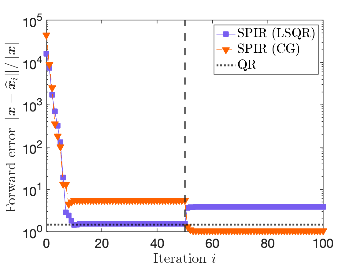
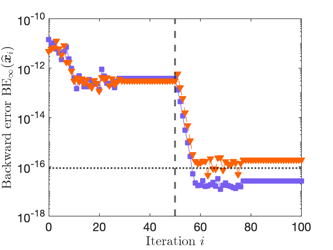
Figure 6: Forward error (left) and backward error (right) for LSQR-based (Algorithm 5) and CG-based 6.2 implementations of SPIR on the example from Fig. 1, along with reference errors for Householder QR. SPIR was implemented with an embedding dimension of $d=12n$ and each refinement step was run for 50 iterations, demarcated by a vertical gray line.

We have performed many numerical tests of SPIR and are fairly confident in its backward stability. For brevity, we provide only a single numerical example here; careful implementation and comprehensive numerical evaluation of SPIR is a subject for future work. Figure 6 shows the forward (left) and backward (right) errors for LSQR- and CG-based implementations of SPIR. Both methods are seen to be backward stable, but only after the second refinement step. We note that Fig. 6 shows the CG-based implementation having a slightly lower forward error than the LSQR implementation, but a slightly higher backward error. This behavior is not universal; repeated random experiments show a range of slight differences between these two variants, and neither variant seems to consistently outperform the other in terms of either forward or backward error.

We have now introduced two fast, (empirically) backward stable randomized least-squares solvers, FOSSILS and SPIR. We end by commenting on which to use. With optimal parameters 2.10, both FOSSILS and SPIR achieve the same optimal rate of convergence (in both theory and practice), and we view both methods as promising candidates for deployment in general-purpose software. The benefit of FOSSILS over SPIR is the simplicity of the iteration 3.3, which requires slightly fewer operations and is easier to parallelize than LSQR or CG [MSM14]. The advantage of SPIR over FOSSILS is that SPIR is parameter-free, avoiding a failure mode for FOSSILS of setting $\alpha$ and $\beta$ incorrectly. Thus, SPIR is probably preferable to FOSSILS if the embedding dimension $d$ is small (e.g., $d\leq 4n$) or if an embedding $\boldsymbol{S}$ with unknown distortion is used.

Disclaimer

This report was prepared as an account of work sponsored by an agency of the United States Government. Neither the United States Government nor any agency thereof, nor any of their employees, makes any warranty, express or implied, or assumes any legal liability or responsibility for the accuracy, completeness, or usefulness of any information, apparatus, product, or process disclosed, or represents that its use would not infringe privately owned rights. Reference herein to any specific commercial product, process, or service by trade name, trademark, manufacturer, or otherwise does not necessarily constitute or imply its endorsement, recommendation, or favoring by the United States Government or any agency thereof. The views and opinions of authors expressed herein do not necessarily state or reflect those of the United States Government or any agency thereof.

Appendix A Proofs for Section 3

A.1 Proof of Lemma 3.2

Denote the error $\boldsymbol{d}_{i}\coloneqq(\boldsymbol{R}^{-\top}\boldsymbol{A}^{\top}\boldsymbol{A}\boldsymbol{R}^{-1})^{-1}\boldsymbol{c}-\boldsymbol{y}_{i}$, which satisfies the recurrence

$$\begin{bmatrix}\boldsymbol{d}_{i+1}\\ \boldsymbol{d}_{i}\end{bmatrix}=\boldsymbol{T}\begin{bmatrix}\boldsymbol{d}_{i}\\ \boldsymbol{d}_{i-1}\end{bmatrix}-\begin{bmatrix}\boldsymbol{f}_{i}\\ \boldsymbol{0}\end{bmatrix}\quad\text{for }\boldsymbol{T}=\begin{bmatrix}(1+\beta)\mathbf{I}-\alpha\boldsymbol{R}^{-\top}\boldsymbol{A}^{\top}\boldsymbol{A}\boldsymbol{R}^{-1}&-\beta\mathbf{I}\\ \mathbf{I}&\boldsymbol{0}\end{bmatrix}.$$

Therefore, expanding this recurrence and using the initial conditions $\boldsymbol{d}_{1}=\boldsymbol{d}_{0}=\boldsymbol{c}$, we obtain

$$\begin{bmatrix}\boldsymbol{d}_{i}\\ \boldsymbol{d}_{i-1}\end{bmatrix}=\boldsymbol{T}^{i-1}\begin{bmatrix}\boldsymbol{c}\\ \boldsymbol{c}\end{bmatrix}+\sum_{j=1}^{i-1}\boldsymbol{T}^{i-1-j}\begin{bmatrix}\boldsymbol{f}_{j}\\ \boldsymbol{0}\end{bmatrix}.$$

From the proof of [Epp24, Thm. 10], we have the bound $\left\|\boldsymbol{T}^{k}\right\|\leq 4(k+1)\eta^{k-1}$. Thus, we have

$$\left\|\boldsymbol{d}_{i}\right\| \leq\left\|\begin{bmatrix}\boldsymbol{d}_{i}\\ \boldsymbol{d}_{i-1}\end{bmatrix}\right\|\leq\left\|\boldsymbol{T}^{i-1}\right\|\left\|\begin{bmatrix}\boldsymbol{c}\\ \boldsymbol{c}\end{bmatrix}\right\|+\sum_{j=0}^{i-1}\left\|\boldsymbol{T}^{i-1-j}\right\|\left\|\begin{bmatrix}\boldsymbol{f}_{j}\\ \boldsymbol{0}\end{bmatrix}\right\|$$

$$\leq 4\sqrt{2}\cdot i\eta^{i-2}\left\|\boldsymbol{c}\right\|+\left(1+4\sum_{j=1}^{i-2}(i-j)\eta^{(i-2)-j}\right)\cdot\max_{1\leq j\leq i-1}\left\|\boldsymbol{f}_{j}\right\|$$

$$\leq 4\sqrt{2}\cdot i\eta^{i-2}\left\|\boldsymbol{c}\right\|+\frac{9}{(1-\eta)^{2}}\cdot\max_{1\leq j\leq i-1}\left\|\boldsymbol{f}_{j}\right\|.$$

We have established the desired conclusion. ∎

A.2 Proof of Theorem 3.1

By 3.1, we have that

$$\boldsymbol{x}=\boldsymbol{x}_{0}+\boldsymbol{R}^{-1}\left(\boldsymbol{R}^{-\top}\boldsymbol{A}^{\top}\boldsymbol{A}\boldsymbol{R}^{-1}\right)^{-1}\boldsymbol{R}^{-\top}\boldsymbol{A}^{\top}(\boldsymbol{b}-\boldsymbol{A}\boldsymbol{x}_{0}).$$

Thus,

$$\boldsymbol{x}-\boldsymbol{x}_{1}=\boldsymbol{R}^{-1}\left(\left(\boldsymbol{R}^{-\top}\boldsymbol{A}^{\top}\boldsymbol{A}\boldsymbol{R}^{-1}\right)^{-1}\boldsymbol{R}^{-\top}\boldsymbol{A}^{\top}(\boldsymbol{b}-\boldsymbol{A}\boldsymbol{x}_{0})-\boldsymbol{y}_{i}\right).$$ (A.1)

By Lemma 3.2, we have

$$\left\|\left(\boldsymbol{R}^{-\top}\boldsymbol{A}^{\top}\boldsymbol{A}\boldsymbol{R}^{-1}\right)^{-1}\boldsymbol{R}^{-\top}\boldsymbol{A}^{\top}(\boldsymbol{b}-\boldsymbol{A}\boldsymbol{x}_{0})-\boldsymbol{y}_{i}\right\|\leq 4\sqrt{2}\cdot i\eta^{i-2}\left\|\boldsymbol{R}^{-\top}\boldsymbol{A}^{\top}(\boldsymbol{b}-\boldsymbol{A}\boldsymbol{x}_{0})\right\|.$$

By Fact 2.3 and the identity $\boldsymbol{A}^{\top}(\boldsymbol{b}-\boldsymbol{A}\boldsymbol{x}_{0})=\boldsymbol{A}^{\top}\boldsymbol{A}(\boldsymbol{x}-\boldsymbol{x}_{0})$, the right-hand side can further be bounded as

$$\left\|\left(\boldsymbol{R}^{-\top}\boldsymbol{A}^{\top}\boldsymbol{A}\boldsymbol{R}^{-1}\right)^{-1}\boldsymbol{R}^{-\top}\boldsymbol{A}^{\top}(\boldsymbol{b}-\boldsymbol{A}\boldsymbol{x}_{0})-\boldsymbol{y}_{i}\right\|\leq\frac{4\sqrt{2}}{1-\eta}\cdot i\eta^{i-2}\cdot\left\|\boldsymbol{A}(\boldsymbol{x}-\boldsymbol{x}_{0})\right\|.$$

Thus, plugging into A.1 and using Fact 2.3, we obtain

$$\left\|\boldsymbol{x}-\boldsymbol{x}_{1}\right\| \leq\left\|\boldsymbol{R}^{-1}\right\|\cdot\frac{4\sqrt{2}\cdot i\eta^{i-2}}{1-\eta}\left\|\boldsymbol{A}(\boldsymbol{x}-\boldsymbol{x}_{0})\right\|\leq\kappa\cdot\frac{4\sqrt{2}}{1-\eta}\cdot i\eta^{i-2}\cdot\left\|\boldsymbol{A}(\boldsymbol{x}-\boldsymbol{x}_{0})\right\|,$$

$$\left\|\boldsymbol{A}(\boldsymbol{x}-\boldsymbol{x}_{1})\right\| \leq\left\|\boldsymbol{A}\boldsymbol{R}^{-1}\right\|\cdot\frac{4\sqrt{2}\cdot i\eta^{i-2}}{1-\eta}\left\|\boldsymbol{A}(\boldsymbol{x}-\boldsymbol{x}_{0})\right\|\leq\frac{4\sqrt{2}}{1-\eta}\cdot i\eta^{i-2}\cdot\left\|\boldsymbol{A}(\boldsymbol{x}-\boldsymbol{x}_{0})\right\|.$$

The bounds 3.4 then follow from bounds on $\left\|\boldsymbol{A}(\boldsymbol{x}-\boldsymbol{x}_{0})\right\|$ for the sketch-and-solve solution [Epp24, Fact 4]. ∎

A.3 Proof of Proposition 3.4

The proof is essentially the same as [DEF⁺23, Thm. 2.3]. For conciseness, drop the subscript $\theta$ for the quantities $\widehat{\operatorname{BE}}_{\theta}$ and $\widehat{\operatorname{BE}}_{\theta,{\rm sk}}$. The squared ratio of the Karlson–Waldén estimate and its sketched variant is

$$\left(\frac{\widehat{\operatorname{BE}}_{\rm sk}(\boldsymbol{\widehat{x}})}{\widehat{\operatorname{BE}}(\boldsymbol{\widehat{x}})}\right)^{2}=\frac{\boldsymbol{z}^{\top}\left((\boldsymbol{S}\boldsymbol{A})^{\top}(\boldsymbol{S}\boldsymbol{A})+\alpha\mathbf{I}\right)^{-1}\boldsymbol{z}}{\boldsymbol{z}^{\top}\left(\boldsymbol{A}^{\top}\boldsymbol{A}+\alpha\mathbf{I}\right)^{-1}\boldsymbol{z}}\quad\text{with }\alpha=\frac{\theta^{2}\left\|\boldsymbol{b}-\boldsymbol{A}\boldsymbol{\widehat{x}}\right\|^{2}}{1+\theta^{2}\left\|\boldsymbol{\widehat{x}}\right\|^{2}},\>\boldsymbol{z}=\boldsymbol{A}^{\top}(\boldsymbol{b}-\boldsymbol{A}\boldsymbol{\widehat{x}}).$$

By the Rayleigh–Ritz principle [Par98, Ch. 8] and some algebra, we have

$$\left(\frac{\widehat{\operatorname{BE}}_{\rm sk}(\boldsymbol{\widehat{x}})}{\widehat{\operatorname{BE}}(\boldsymbol{\widehat{x}})}\right)^{2}\leq\lambda_{\rm max}\left(\left(\boldsymbol{A}^{\top}\boldsymbol{A}+\alpha\mathbf{I}\right)^{1/2}\left((\boldsymbol{S}\boldsymbol{A})^{\top}(\boldsymbol{S}\boldsymbol{A})+\alpha\mathbf{I}\right)^{-1}\left(\boldsymbol{A}^{\top}\boldsymbol{A}+\alpha\mathbf{I}\right)^{1/2}\right).$$

Therefore,

$$\left(\frac{\widehat{\operatorname{BE}}(\boldsymbol{\widehat{x}})}{\widehat{\operatorname{BE}}_{\rm sk}(\boldsymbol{\widehat{x}})}\right)^{2}\geq\lambda_{\rm min}\left(\left(\boldsymbol{A}^{\top}\boldsymbol{A}+\alpha\mathbf{I}\right)^{-1/2}\left((\boldsymbol{S}\boldsymbol{A})^{\top}(\boldsymbol{S}\boldsymbol{A})+\alpha\mathbf{I}\right)\left(\boldsymbol{A}^{\top}\boldsymbol{A}+\alpha\mathbf{I}\right)^{-1/2}\right).$$

Thus, by the Rayleigh–Ritz principle, we have

$$\left(\frac{\widehat{\operatorname{BE}}(\boldsymbol{\widehat{x}})}{\widehat{\operatorname{BE}}_{\rm sk}(\boldsymbol{\widehat{x}})}\right)^{2}\geq\min_{\boldsymbol{w}\neq\boldsymbol{0}}\frac{\boldsymbol{w}^{\top}\left((\boldsymbol{S}\boldsymbol{A})^{\top}(\boldsymbol{S}\boldsymbol{A})+\alpha\mathbf{I}\right)\boldsymbol{w}}{\boldsymbol{w}^{\top}\left(\boldsymbol{A}^{\top}\boldsymbol{A}+\alpha\mathbf{I}\right)\boldsymbol{w}}\geq\min\left\{\min_{\boldsymbol{w}\neq\boldsymbol{0}}\frac{\left\|\boldsymbol{S}\boldsymbol{A}\boldsymbol{w}\right\|^{2}}{\left\|\boldsymbol{A}\boldsymbol{w}\right\|^{2}},1\right\}.$$

The second inequality is a consequence of the numerical inequality $(a+x)/(1+x)\geq\min\{1,a\}$. Finally, invoking the QR decomposition 2.4 and Fact 2.3, we continue

$$\left(\frac{\widehat{\operatorname{BE}}(\boldsymbol{\widehat{x}})}{\widehat{\operatorname{BE}}_{\rm sk}(\boldsymbol{\widehat{x}})}\right)^{2}\geq\min\left\{\min_{\boldsymbol{w}\neq\boldsymbol{0}}\frac{\left\|\boldsymbol{R}\boldsymbol{w}\right\|^{2}}{\left\|\boldsymbol{A}\boldsymbol{w}\right\|^{2}},1\right\}=\min\left\{\frac{1}{\sigma_{\rm max}^{2}(\boldsymbol{A}\boldsymbol{R}^{-1})},1\right\}\geq(1-\eta)^{2}.$$

Combining this result with Fact 3.3 implies the desired lower bound. The desired upper bound is proven similarly. ∎

A.4 Proof of Theorem 3.5

Let us compute the Karlson–Waldén estimate $\widehat{\operatorname{BE}}_{1}(\boldsymbol{\widehat{x}})$. Expand $\boldsymbol{\widehat{x}}=\sum_{i=1}^{n}(\boldsymbol{v}_{i}^{\top}\boldsymbol{\widehat{x}})\boldsymbol{v}_{i}^{\vphantom{\top}}$, we have

$$\boldsymbol{A}^{\top}(\boldsymbol{b}-\boldsymbol{A}\boldsymbol{\widehat{x}})=\sum_{i=1}^{n}\sigma_{i}^{\vphantom{\top}}\left(\boldsymbol{u}_{i}^{\top}\boldsymbol{b}-\sigma_{i}^{\vphantom{\top}}(\boldsymbol{v}_{i}^{\top}\boldsymbol{\widehat{x}})\right)\boldsymbol{v}_{i}^{\vphantom{\top}}=\boldsymbol{A}^{\top}(\boldsymbol{b}-\boldsymbol{A}\boldsymbol{\widehat{x}})=\sum_{i=1}^{n}\sigma_{i}^{2}\boldsymbol{v}_{i}^{\top}(\boldsymbol{x}-\boldsymbol{\widehat{x}})\cdot\boldsymbol{v}_{i}^{\vphantom{\top}}.$$

For the second equality, we used the fact that the true solution $\boldsymbol{x}$ to the least-squares proble satisfies $\boldsymbol{u}_{i}^{\top}\boldsymbol{b}=\sigma_{i}^{\vphantom{\top}}\boldsymbol{v}_{i}^{\top}\boldsymbol{x}$. We now evaluate the matrix expression in the Karlson–Waldén estimate:

$$\left(\boldsymbol{A}^{\top}\boldsymbol{A}+\frac{\left\|\boldsymbol{b}-\boldsymbol{A}\boldsymbol{\widehat{x}}\right\|^{2}}{1+\left\|\boldsymbol{\widehat{x}}\right\|^{2}}\mathbf{I}\right)^{-1/2}=\sum_{i=1}^{n}\left(\sigma_{i}^{2}+\frac{\left\|\boldsymbol{b}-\boldsymbol{A}\boldsymbol{\widehat{x}}\right\|^{2}}{1+\left\|\boldsymbol{\widehat{x}}\right\|^{2}}\right)^{-1/2}\boldsymbol{v}_{i}^{\vphantom{\top}}\boldsymbol{v}_{i}^{\top}$$

Combining the two previous displays and simplifying yields

$$\widehat{\operatorname{BE}}_{1}(\boldsymbol{\widehat{x}})^{2}=\sum_{i=1}^{n}\frac{\sigma_{i}^{4}}{(1+\left\|\boldsymbol{\widehat{x}}\right\|^{2})\sigma_{i}^{2}+\left\|\boldsymbol{b}-\boldsymbol{A}\boldsymbol{\widehat{x}}\right\|^{2}}\left(\boldsymbol{v}_{i}^{\top}(\boldsymbol{x}-\boldsymbol{\widehat{x}})\right)^{2}.$$ (A.2)

Now, we make a change of deductions. By Fact 3.3, $\operatorname{BE}_{1}(\boldsymbol{\widehat{x}})\lesssim\varepsilon$ if and only if $\widehat{\operatorname{BE}}_{1}(\boldsymbol{\widehat{x}})\lesssim\varepsilon$. This, in turn, occurs if and only if each summand in A.2 satisfies

$$\frac{\sigma_{i}^{4}}{(1+\left\|\boldsymbol{\widehat{x}}\right\|^{2})\sigma_{i}^{2}+\left\|\boldsymbol{b}-\boldsymbol{A}\boldsymbol{\widehat{x}}\right\|^{2}}\left(\boldsymbol{v}_{i}^{\top}(\boldsymbol{x}-\boldsymbol{\widehat{x}})\right)^{2}\lesssim\varepsilon^{2}\quad\text{for }i=1,2,\ldots,n.$$ (A.3)

Rearranging and using the comparison $\sqrt{\alpha+\beta}\asymp\sqrt{\alpha}+\sqrt{\beta}$, we see that A.3 holds if and only if

$$\left|\boldsymbol{v}_{i}^{\top}(\boldsymbol{x}-\boldsymbol{\widehat{x}})\right|\lesssim\frac{1}{\sigma_{i}}(1+\left\|\boldsymbol{\widehat{x}}\right\|)\varepsilon+\frac{1}{\sigma_{i}^{2}}\left\|\boldsymbol{b}-\boldsymbol{A}\boldsymbol{\widehat{x}}\right\|\varepsilon.$$

This is the desired conclusion 3.8, under the standing normalization $\left\|\boldsymbol{A}\right\|=\left\|\boldsymbol{b}\right\|=1$. ∎

Appendix B Prony’s method and quantum eigenvalue algorithms

Recently, there has been interest in using frequency estimation algorithms such as Prony’s method, the matrix pencil method [KMC⁺22], and ESPRIT [LNY23, DELZ24] to compute eigenvalues with quantum computers. We will consider the simplest of these, Prony’s method, shown in Algorithm 6. Observe that Prony’s method involves two least-squares solves, which could be tackled with randomized methods. We mention off-handedly that there exist structure-exploiting least-squares solvers for Toeplitz [XXCB14] and Vandermonde [WEB24] least-squares problems with an asympotically faster $\mathcal{O}(m\log^{2}n\log^{2}(1/u))$ runtime; these algorithms might or might not be faster than randomized methods for small values of $n$.

Algorithm 6 Prony’s method

1:Noisy measurements of the form $f_{j}=\sum_{i=1}^{n}\mu_{i}z_{i}^{j}+\varepsilon_{j}\in\mathbb{C}$ for $0\leq j\leq m+n-1$

2:Vectors of estimates $\boldsymbol{\widehat{\mu}},\boldsymbol{\widehat{z}}\in\mathbb{C}^{n}$ with $\widehat{z}_{i}\approx z_{i}$, $\widehat{\mu}_{i}\approx\mu_{i}$ (up to permutation)

3:Form $\boldsymbol{A}=(f_{n-1+(i-j)})_{1\leq i\leq m,1\leq j\leq n}$ and $\boldsymbol{b}=(f_{n-1+i})_{1\leq i\leq m}$

4:$\boldsymbol{p}\leftarrow\textsc{LeastSquaresSolver}(\boldsymbol{A},\boldsymbol{b})$

5:$\boldsymbol{\widehat{z}}\leftarrow\textsc{PolynomialRoots}(z^{n}-p_{1}z^{n-1}-p_{2}z^{n-2}-\cdots-p_{n}z^{0})$

6:Form $\boldsymbol{A}=(z_{j}^{i-1})_{1\leq i\leq m+n,1\leq j\leq n}$ and $\boldsymbol{b}=(f_{i-1})_{1\leq i\leq m+n}$

7:$\boldsymbol{\widehat{\mu}}\leftarrow\textsc{LeastSquaresSolver}(\boldsymbol{A},\boldsymbol{b})$

Prony’s method can used to estimate eigenvalues of a Hermitian matrix $\boldsymbol{H}$ as follows. Suppose we use a quantum computer to collect measurements of the form

$$f_{j}=\boldsymbol{x}_{0}^{*}\mathrm{e}^{-\mathrm{i}(\Delta t)j\boldsymbol{H}}\boldsymbol{x}_{0}^{\vphantom{*}}+\varepsilon_{j}\quad\text{for }j=0,\ldots,t,$$

where $\boldsymbol{x}_{0}$ is an appropriately chosen vector and $\varepsilon_{j}$ are independent random errors. By running Prony’s method on this data and normalizing the outputs to have unit modulus $\widehat{z}_{i}/|\widehat{z}_{i}|=\mathrm{e}^{-\mathrm{i}(\Delta t)\lambda_{i}}$, we obtain an approximations $\lambda_{i}$ to the eigenvalues of $\boldsymbol{H}$.

With this context, the least-squares problem shown in the right panel of Fig. 4 is constructed as follows. We let $\boldsymbol{H}=\boldsymbol{H}(h)$ be the transverse field Ising mode Hamiltonian on $16$ sites with magnetization $h=1$, choose $\boldsymbol{x}_{0}$ to be the minimum-eigenvalue eigenvector of $\boldsymbol{H}(h=0)$, and set the noise $\varepsilon_{j}$ to be independent complex Gaussians with mean zero and standard deviation $10^{-6}$. In the right panel of Fig. 4, we construct $\boldsymbol{A}$ and $\boldsymbol{b}$ as in line 1 of Algorithm 6; thus, we consider only the first least-squares solve of Prony’s method.

Algorithm 7 FOSSILS: Recommended implementation

1:Matrix $\boldsymbol{A}\in^{m\times n}$, right-hand side $\boldsymbol{b}\in^{m}$

2:Backward stable least-squares solution $\boldsymbol{x}\in^{n}$

3:$\boldsymbol{d}\leftarrow\textsc{ColumnNorms}(\boldsymbol{A})$, $\boldsymbol{A}\leftarrow\boldsymbol{A}\operatorname{diag}(\boldsymbol{d})^{-1}$ $\vartriangleright$ Normalize columns

4:$d\leftarrow 12n$, $\zeta\leftarrow 8$ $\vartriangleright$ Parameters for embedding

5:$\beta\leftarrow d/n$, $\alpha\leftarrow(1-\beta)^{2}$ $\vartriangleright$ Or $\beta=1.2\cdot d/n$, to be safe

6:$\boldsymbol{S}\leftarrow\textsc{SparseSignEmbedding}(m,d,\zeta)$

7:$(\boldsymbol{U},\boldsymbol{\Sigma},\boldsymbol{V})\leftarrow\textsc{SVD}(\boldsymbol{S}\boldsymbol{A})$ $\vartriangleright$ Sketch and SVD

8:$\mathrm{normest}\leftarrow\boldsymbol{\Sigma}(1,1)$, $\mathrm{condest}\leftarrow\boldsymbol{\Sigma}(1,1)/\boldsymbol{\Sigma}(n,n)$

9:if $\mathrm{condest}>1/(30u)$ then

10:     Print “Warning! Condition number estimate is $\langle\mathrm{condest}\rangle$”

11:     $\mu\leftarrow 10\left\|\boldsymbol{A}\right\|_{\rm F}u$, $\boldsymbol{\Sigma}_{\rm reg}\leftarrow(\boldsymbol{\Sigma}^{2}+\mu^{2}\mathbf{I})^{1/2}$ $\vartriangleright$ Add regularization if rank deficient

12:else

13:     $\mu\leftarrow 0$, $\boldsymbol{\Sigma}_{\rm reg}\leftarrow\boldsymbol{\Sigma}$

14:end if

15:$\boldsymbol{x}\leftarrow\boldsymbol{V}(\boldsymbol{\Sigma}^{-1}(\boldsymbol{U}^{\top}(\boldsymbol{S}\boldsymbol{b})))$ $\vartriangleright$ Sketch-and-solve initialization

16:$\boldsymbol{r}\leftarrow\boldsymbol{b}-\boldsymbol{A}\boldsymbol{x}$

17:$\boldsymbol{P}\leftarrow\boldsymbol{V}\boldsymbol{\Sigma}_{\rm reg}^{-1}$ $\vartriangleright$ Preconditioner, taking the role of $\boldsymbol{R}^{-1}$

18:for $i=0,1$ do $\vartriangleright$ Two steps of iterative refinement with inner solver

19:     $\boldsymbol{y},\boldsymbol{y}_{\rm old},\boldsymbol{c}\leftarrow\boldsymbol{P}^{\top}(\boldsymbol{A}^{\top}(\boldsymbol{b}-\boldsymbol{A}\boldsymbol{x}_{i})$

20:     for $j=0,1,\ldots,99$ do $\vartriangleright$ Polyak heavy ball method, 100 iterations max

21:         $\boldsymbol{z}\leftarrow\boldsymbol{P}\boldsymbol{y}$

22:         $\boldsymbol{\delta}\leftarrow\alpha(\boldsymbol{c}-\boldsymbol{P}^{\top}(\boldsymbol{A}^{\top}(\boldsymbol{A}\boldsymbol{z}))+\mu^{2}\boldsymbol{z})+\beta(\boldsymbol{y}-\boldsymbol{y}_{\rm old})$

23:         $(\boldsymbol{y},\boldsymbol{y}_{\rm old})\leftarrow(\boldsymbol{y}+\boldsymbol{\delta},\boldsymbol{y})$

24:         if $i=0$ and $\left\|\boldsymbol{\delta}\right\|\leq(10\cdot\mathrm{normest}\cdot\left\|\boldsymbol{x}\right\|+0.4\cdot\mathrm{condest}\cdot\left\|\boldsymbol{r}\right\|)u$ then

25:              break $\vartriangleright$ Break after update is small during first inner solve

26:         else if $i=1$ and $\textsc{Mod}(i,5)=0$ then $\vartriangleright$ Check backward error every five iterations

27:              $\boldsymbol{\widehat{x}}\leftarrow\boldsymbol{x}+\boldsymbol{P}\boldsymbol{y}$

28:              $\boldsymbol{\widehat{r}}\leftarrow\boldsymbol{b}-\boldsymbol{A}\boldsymbol{\widehat{x}}$

29:              $\theta\leftarrow\left\|\boldsymbol{A}\right\|_{\rm F}/\left\|\boldsymbol{b}\right\|$

30:              $\widehat{\mathrm{BE}}_{\rm sk}\leftarrow\tfrac{\theta}{\sqrt{1+\theta^{2}\left\|\boldsymbol{\widehat{x}}\right\|^{2}}}\cdot\left\|(\boldsymbol{\Sigma}^{2}+\tfrac{\theta^{2}\left\|\boldsymbol{\widehat{r}}\right\|^{2}}{1+\theta^{2}\left\|\boldsymbol{\widehat{x}}\right\|^{2}}\mathbf{I})^{-1/2}\boldsymbol{V}^{\top}(\boldsymbol{A}^{\top}\boldsymbol{\widehat{r}})\right\|$ $\vartriangleright$ Sketched KW estimate 3.6

31:              if $\widehat{\mathrm{BE}}_{\rm sk}<\left\|\boldsymbol{A}\right\|_{\rm F}u$ then

32:                  break $\vartriangleright$ Break when backward stability achieved during second inner solve

33:              end if

34:         end if

35:     end for

36:     $\boldsymbol{x}\leftarrow\boldsymbol{x}+\boldsymbol{P}\boldsymbol{y}$ $\vartriangleright$ Iterative refinement

37:end for

38:$\boldsymbol{x}\leftarrow\operatorname{diag}(\boldsymbol{d})^{-1}\boldsymbol{x}$ $\vartriangleright$ Undo column scaling

References

• [AMT10] Haim Avron, Petar Maymounkov, and Sivan Toledo. Blendenpik: Supercharging LAPACK’s Least-Squares Solver. SIAM Journal on Scientific Computing, 32(3):1217–1236, January 2010. doi:10.1137/090767911.
• [Bjö96] Åke Björck. Numerical Methods for Least Squares Problems. SIAM, 1996.
• [BSW14] P. Baldi, P. Sadowski, and D. Whiteson. Searching for exotic particles in high-energy physics with deep learning. Nature Communications, 5(1):4308, July 2014. doi:10.1038/ncomms5308.
• [CD24] Erin Carson and Ieva Daužickaitė. A comparison of mixed precision iterative refinement approaches for least-squares problems, may 2024. https://arxiv.org/abs/2405.18363.
• [CDD+23] Younghyun Cho, James W. Demmel, Michał Dereziński, Haoyun Li, Hengrui Luo, Michael W. Mahoney, and Riley J. Murray. Surrogate-based autotuning for randomized sketching algorithms in regression problems, August 2023. https://arxiv.org/abs/2308.15720.
• [CDDR23] Shabarish Chenakkod, Michał Dereziński, Xiaoyu Dong, and Mark Rudelson. Optimal embedding dimension for sparse subspace embeddings, November 2023. https://arxiv.org/abs/2311.10680.
• [Coh16] Michael B. Cohen. Nearly tight oblivious subspace embeddings by trace inequalities. In Proceedings of the Twenty-Seventh Annual ACM-SIAM Symposium on Discrete Algorithms, pages 278–287. Society for Industrial and Applied Mathematics, January 2016. doi:10.1137/1.9781611974331.ch21.
• [DDH07] James Demmel, Ioana Dumitriu, and Olga Holtz. Fast linear algebra is stable. Numerische Mathematik, 108(1):59–91, October 2007. doi:10.1007/s00211-007-0114-x.
• [DEF+23] Mateo Díaz, Ethan N. Epperly, Zachary Frangella, Joel A. Tropp, and Robert J. Webber. Robust, randomized preconditioning for kernel ridge regression, April 2023. https://arxiv.org/abs/2304.12465.
• [DELZ24] Zhiyan Ding, Ethan N. Epperly, Lin Lin, and Ruizhe Zhang. The ESPRIT algorithm under high noise: Optimal error scaling and noisy super-resolution, April 2024. https://arxiv.org/abs/2404.03885.
• [DH11] Timothy Davis and Yifan Hu. The University of Florida sparse matrix collection. ACM Transactions on Mathematical Software (TOMS), 38(1):1–25, 2011. doi:10.1145/2049662.2049663.
• [DM23] Yijun Dong and Per-Gunnar Martinsson. Simpler is better: A comparative study of randomized pivoting algorithms for CUR and interpolative decompositions. Advances in Computational Mathematics, 49(4):66, August 2023. doi:10.1007/s10444-023-10061-z.
• [Epp24] Ethan N. Epperly. Fast and forward stable randomized algorithms for linear least-squares problems. SIAM Journal on Matrix Analysis and Applications, to appear, 2024. preprint available at https://arxiv.org/abs/2311.04362v2.
• [ET24] Ethan N Epperly and Joel A Tropp. Efficient error and variance estimation for randomized matrix computations. SIAM Journal on Scientific Computing, 46(1):A508–A528, 2024. doi:10.1137/23M1558537.
• [GJT12] Serge Gratton, Pavel Jiránek, and David Titley-Peloquin. On the accuracy of the Karlson–Waldén estimate of the backward error for linear least squares problems. SIAM Journal on Matrix Analysis and Applications, 33(3):822–836, January 2012. doi:10.1137/110825467.
• [Grc03] Joseph F. Grcar. Optimal sensitivity analysis of linear least squares. Lawrence Berkeley National Laboratory, Report LBNL-52434, 99, 2003. https://ccse.lbl.gov/Publications/sepp/leastSquares/LBNL-52434.pdf.
• [Gre89] Anne Greenbaum. Behavior of slightly perturbed Lanczos and conjugate-gradient recurrences. Linear Algebra and its Applications, 113:7–63, 1989. doi:10.1016/0024-3795(89)90285-1.
• [Gre97] Anne Greenbaum. Estimating the attainable accuracy of recursively computed residual methods. SIAM Journal on Matrix Analysis and Applications, 18(3):535–551, July 1997. doi:10.1137/S0895479895284944.
• [GSS07] Joseph F. Grcar, Michael A. Saunders, and Zheng Su. Estimates of optimal backward perturbations for linear least squares problems. Technical report, Lawrence Berkeley National Lab, 2007.
• [Gu98] Ming Gu. Backward perturbation bounds for linear least squares problems. SIAM Journal on Matrix Analysis and Applications, 20(2):363–372, January 1998. doi:10.1137/S0895479895296446.
• [GW66] Gene H Golub and James H Wilkinson. Note on the iterative refinement of least squares solution. Numer. Math., 9(2):139–148, 1966. doi:10.1007/BF02166032.
• [Hig02] Nicholas J Higham. Accuracy and Stability of Numerical Algorithms. SIAM, 2002.
• [HM19] Nicholas J. Higham and Theo Mary. A new approach to probabilistic rounding error analysis. SIAM Journal on Scientific Computing, 41(5):A2815–A2835, January 2019. doi:10.1137/18M1226312.
• [HMT11] Nathan Halko, Per-Gunnar Martinsson, and Joel A. Tropp. Finding structure with randomness: Probabilistic algorithms for constructing approximate matrix decompositions. SIAM Review, 53(2):217–288, January 2011. doi:10.1137/090771806.
• [KMC+22] Katherine Klymko, Carlos Mejuto-Zaera, Stephen J. Cotton, Filip Wudarski, Miroslav Urbanek, Diptarka Hait, Martin Head-Gordon, K. Birgitta Whaley, Jonathan Moussa, Nathan Wiebe, Wibe A. de Jong, and Norm M. Tubman. Real-time evolution for ultracompact Hamiltonian eigenstates on quantum hardware. PRX Quantum, 3(2):020323, May 2022. doi:10.1103/PRXQuantum.3.020323.
• [KT24] Anastasia Kireeva and Joel A. Tropp. Randomized matrix computations: Themes and variations, February 2024. https://arxiv.org/abs/2402.17873.
• [KW97] Rune Karlson and Bertil Waldén. Estimation of optimal backward perturbation bounds for the linear least squares problem. BIT Numerical Mathematics, 37(4):862–869, December 1997. doi:10.1007/BF02510356.
• [LNY23] Haoya Li, Hongkang Ni, and Lexing Ying. Adaptive low-depth quantum algorithms for robust multiple-phase estimation. Physical Review A, 108(6):062408, December 2023. doi:10.1103/PhysRevA.108.062408.
• [LP20] Jonathan Lacotte and Mert Pilanci. Optimal randomized first-order methods for least-squares problems. In Proceedings of the 37th International Conference on Machine Learning, 2020.
• [LP21] Jonathan Lacotte and Mert Pilanci. Faster least squares optimization, April 2021. https://arxiv.org/abs/1911.02675.
• [MMS18] Cameron Musco, Christopher Musco, and Aaron Sidford. Stability of the Lanczos method for matrix function approximation. In Proceedings of the 2018 Annual ACM-SIAM Symposium on Discrete Algorithms, pages 1605–1624. SIAM, January 2018. doi:10.1137/1.9781611975031.105.
• [MNTW24] Maike Meier, Yuji Nakatsukasa, Alex Townsend, and Marcus Webb. Are sketch-and-precondition least squares solvers numerically stable? SIAM Journal on Matrix Analysis and Applications, 45(2):905–929, 2024. doi:10.1137/23M1551973.
• [MSM14] Xiangrui Meng, Michael A. Saunders, and Michael W. Mahoney. LSRN: A parallel iterative solver for strongly over- or underdetermined systems. SIAM Journal on Scientific Computing, 36(2):C95–C118, January 2014. doi:10.1137/120866580.
• [MT20] Per-Gunnar Martinsson and Joel A. Tropp. Randomized numerical linear algebra: Foundations and algorithms. Acta Numerica, 29:403–572, May 2020. doi:10.1017/S0962492920000021.
• [NT24] Yuji Nakatasukasa and Joel A. Tropp. Fast & accurate randomized algorithms for linear systems and eigenvalue problems. SIAM Journal on Matrix Analysis and Applications, to appear, 2024. preprint available at https://arxiv.org/abs/2111.00113.
• [OPA19] Ibrahim Kurban Ozaslan, Mert Pilanci, and Orhan Arikan. Iterative Hessian sketch with momentum. In IEEE International Conference on Acoustics, Speech and Signal Processing 2019, pages 7470–7474, 2019. doi:10.1109/ICASSP.2019.8682720.
• [Pai76] Christopher C. Paige. Error analysis of the Lanczos algorithm for tridiagonalizing a symmetric matrix. IMA Journal of Applied Mathematics, 18(3):341–349, 1976. doi:10.1093/imamat/18.3.341.
• [Pai24] Christopher C. Paige. Analyzing Vector Orthogonalization Algorithms. SIAM Journal on Matrix Analysis and Applications, pages 829–846, June 2024. doi:10.1137/22M1519523.
• [Par98] B. N. Parlett. The Symmetric Eigenvalue Problem. SIAM, 1998.
• [Pol64] Boris T. Polyak. Some methods of speeding up the convergence of iteration methods. Ussr computational mathematics and mathematical physics, 4(5):1–17, 1964. doi:10.1016/0041-5553(64)90137-5.
• [PS82] Christopher C. Paige and Michael A. Saunders. LSQR: An Algorithm for Sparse Linear Equations and Sparse Least Squares. ACM Transactions on Mathematical Software, 8(1):43–71, March 1982. doi:10.1145/355984.355989.
• [PW16] Mert Pilanci and Martin J. Wainwright. Iterative Hessian sketch: Fast and accurate solution approximation for constrained least-squares. The Journal of Machine Learning Research, 17(1):1842–1879, 2016.
• [RT08] Vladimir Rokhlin and Mark Tygert. A fast randomized algorithm for overdetermined linear least-squares regression. Proceedings of the National Academy of Sciences, 105(36):13212–13217, September 2008. doi:10.1073/pnas.0804869105.
• [Sar06] Tamás Sarlós. Improved approximation algorithms for large matrices via random projections. In 2006 47th Annual IEEE Symposium on Foundations of Computer Science, pages 143–152, October 2006. doi:10.1109/FOCS.2006.37.
• [Ste98] G. W. Stewart. Matrix Algorithms Volume I: Basic decompositions. SIAM, 1998.
• [TW23] Joel A. Tropp and Robert J. Webber. Randomized algorithms for low-rank matrix approximation: Design, analysis, and applications, June 2023. https://arxiv.org/abs/2306.12418.
• [TYUC19] Joel A. Tropp, Alp Yurtsever, Madeleine Udell, and Volkan Cevher. Streaming low-rank matrix approximation with an application to scientific simulation. SIAM Journal on Scientific Computing, 41(4):A2430–A2463, January 2019. doi:10.1137/18M1201068.
• [VDS69] A. Van Der Sluis. Condition numbers and equilibration of matrices. Numerische Mathematik, 14(1):14–23, 1969. doi:10.1007/BF02165096.
• [WEB24] Heather Wilber, Ethan N. Epperly, and Alex H. Barnett. A superfast direct inversion method for the nonuniform discrete Fourier transform, April 2024. https://arxiv.org/abs/2404.13223.
• [Wed73] Per-Åke Wedin. Perturbation theory for pseudo-inverses. BIT Numerical Mathematics, 13(2):217–232, June 1973. doi:10.1007/BF01933494.
• [WKS95] Bertil Waldén, Rune Karlson, and Ji-Guang Sun. Optimal backward perturbation bounds for the linear least squares problem. Numerical Linear Algebra with Applications, 2(3):271–286, May 1995. doi:10.1002/nla.1680020308.
• [XXCB14] Yuanzhe Xi, Jianlin Xia, Stephen Cauley, and Venkataramanan Balakrishnan. Superfast and stable structured solvers for Toeplitz least squares via randomized sampling. SIAM Journal on Matrix Analysis and Applications, 35(1):44–72, 2014. doi:10.1137/120895755.