Gaussian Copula Models for Nonignorable Missing Data Using Auxiliary Marginal Quantiles

Abstract

We present an approach for modeling and imputation of nonignorable missing data under Gaussian copulas. The analyst posits a set of quantiles of the marginal distributions of the study variables, for example, reflecting information from external data sources or elicited expert opinion. When these quantiles are accurately specified, we prove it is possible to consistently estimate the copula correlation and perform multiple imputation in the presence of nonignorable missing data. We develop algorithms for estimation and imputation that are computationally efficient, which we evaluate in simulation studies of multiple imputation inferences. We apply the model to analyze associations between lead exposure levels and end-of-grade test scores for 170,000 students in North Carolina. These measurements are not missing at random, as children deemed at-risk for high lead exposure are more likely to be measured. We construct plausible marginal quantiles for lead exposure using national statistics provided by the Centers for Disease Control and Prevention. Complete cases and missing at random analyses appear to underestimate the relationships between certain variables and end-of-grade test scores, while multiple imputation inferences under our model support stronger, adverse associations between lead exposure and educational outcomes.

Keywords: Bayesian; imputation; MNAR; data integration; nonresponse

1 Introduction

The Gaussian copula is a flexible joint distribution for multivariate data. The model can characterize complex dependencies while also capturing non-Gaussian marginal distributions. Methodological advances have made the Gaussian copula compatible with mixed data types (Hoff, , 2007; Feldman and Kowal, , 2022), increased its scalability to high-dimensional variable sets (Murray et al., , 2013), and improved its ability to capture non-linearity and interactions (Feldman and Kowal, , 2024). Because of these appealing features, it has been deployed in numerous applications including, for example, in economics and finance (Fan and Patton, , 2014), marketing and management (Eckert and Hohberger, , 2023), and political science (Chiba et al., , 2015).

The Gaussian copula can be readily implemented when data have missing values. Indeed, researchers (e.g., Käärik and Käärik, , 2010; Di Lascio et al., , 2015; Zhao and Udell, , 2020; Hollenbach et al., , 2021; Hoff, , 2022; Christoffersen et al., , 2023) have suggested Gaussian copulas as multivariate, joint modeling engines for (multiple) imputation. Existing methods, however, tend to assume that missingness among the study variables is missing completely at random (MCAR) or missing at random (MAR) (Rubin, , 1976). We are not aware of methodology for itemwise nonignorable missingness with Gaussian copula models.

In this article, we develop a framework to handle nonignorable missing data in Gaussian copula models. Our general strategy is to specify a Bayesian Gaussian copula model that includes both the study variables and the missingness indicators, coupled with auxiliary information on the marginal distributions of the study variables. Using this strategy, we prove that analysts need to know only a small, arbitrary set of auxiliary marginal quantiles to enable consistent estimation of the copula correlation; entire distributions are not necessary. These results hold for a version of an additive nonignorable (AN) missingness mechanism (Hirano et al., , 2001; Sadinle and Reiter, , 2019). This mechanism allows the reason for missingness in a variable potentially to depend on the value of the variable itself. We develop algorithms for estimating the copula correlation that result in significant computational gains relative to alternative copula models, which allows fitting to scale to data with (moderately) large sample sizes in reasonable time using typical computational setups. We also present strategies for estimating other quantiles of the marginal distributions beyond those in the auxiliary information. Our approach provides uncertainty quantification for the unknown marginals, which we utilize for multiple imputation (Rubin, , 1987).

We develop the methodology for settings where marginal quantiles for variables subject to missingness are available in external data sources. For example, previewing the application in Section 5, suppose an analysis involving health measurements suffers from nonignorable missingness, e.g., people likely to have unconcerning values are not measured. For many health measurements, there exists information on marginal quantiles from national benchmark surveys or administrative databases. We seek to use the auxiliary quantiles to adjust for nonignorable missingness in the analysis at hand. When auxiliary quantiles are not available or known precisely, analysts can posit different plausible marginal quantiles and assess the sensitivity of ultimate analyses under those specifications, e.g., via multiple imputation analyses. We note that the use of known marginal distributions for imputation of nonignorable missing data also has been proposed for categorical data models (Pham et al., , 2018; Akande et al., , 2021; Deng et al., , 2013; Si et al., , 2015, 2016; Tang et al., , 2024), but not for continuous and mixed variables like we do here.

We apply the methodology in data comprising health, socioeconomic, demographic and educational measurements collected on over 170,000 North Carolina children. Among the study variables are end-of-grade math and reading test scores and a measure of lead exposure, the latter of which is subject to abundant missingness that is likely nonignorable. The state requires children at high risk of lead exposure to be measured, but not children at low risk of lead exposure. To inform the imputation of the missing values, we leverage marginal quantiles on lead exposure published by the Centers for Disease Control and Prevention. Using this information, we find lead exposure apparently is more adversely associated with test scores than suggested from complete cases or MAR analyses.

The remainder of this article is organized as follows. In Section 2, we present the Gaussian copula model with nonignorable missing data and information on marginal distributions. Here we present two theoretical results, namely (i) that fully specified marginal distributions provide posterior consistency of the copula correlation in the presence of nonignorable missingness, and (ii) a derivation that the Gaussian copula implies a version of the AN missingness mechanism. In Section 3, we modify the copula model and develop imputation strategies for settings where the auxiliary marginal information constitutes a specified set of marginal quantiles. Here we present our main theorem: under the AN missingness mechanism, this limited auxiliary information still allows consistent estimation of the copula correlation. In Section 4, we present simulations studying the effect of differing amounts of auxiliary quantiles and repeated sampling properties of multiple imputation inferences with the model. In Section 5, we present the analysis of the North Carolina lead exposure data. In Section 6, we summarize and suggest research directions. Codes for all analyses are available at https://github.com/jfeldman396/EHQL-Impute.

2 Gaussian Copula with Nonignorable Missing Data

For $i=1,\dots,n$ individuals, let $\boldsymbol{y}_{i}=(y_{i1},\dots,y_{ip})$ comprise measurements on $p$ study variables. Let $\boldsymbol{y}=\{\boldsymbol{y}_{i}:i=1,\dots,n\}$. When $\boldsymbol{y}$ contains missing values, let $r_{ij}=1$ when $y_{ij}$ is missing, and $r_{ij}=0$ otherwise. Let $\boldsymbol{r}_{i}=\{r_{i1},\dots,r_{ip}\}$ for $i=1,\dots,n$, and $\boldsymbol{r}=\{\boldsymbol{r}_{i}:i=1,\dots,n\}$. We refer to the study variables using $Y=(Y_{1},\dots,Y_{p})$ and nonresponse indicators using $R=(R_{1},\dots,R_{p})$. When the missingness is nonignorable, we require a model for the joint distribution of $(\boldsymbol{y},\boldsymbol{r})$. To aid specification of this distribution, we partition the data into observed and missing components, $\boldsymbol{y}=(\boldsymbol{y}^{obs},\boldsymbol{y}^{mis})$, where $\boldsymbol{y}^{obs}=\{y_{ij}:r_{ij}=0;i=1,\dots,n;j=1,\dots,p\}$ and $\boldsymbol{y}^{mis}=\{y_{ij}:r_{ij}=1;i=1,\dots,n;j=1,\dots,p\}$. Then, the two principal modeling tasks are to specify the distribution of the observed data,

$$p(\boldsymbol{y}^{obs},\boldsymbol{r}\mid\boldsymbol{\gamma})=\int p(\boldsymbol{y}^{obs},\boldsymbol{y}^{mis},\boldsymbol{r}\mid\boldsymbol{\gamma})d\boldsymbol{y}^{mis},$$ (1)

and to impose some identifying restriction on $p(\boldsymbol{y}^{mis}\mid\boldsymbol{y}^{obs},\boldsymbol{r},\boldsymbol{\gamma})$, also known as the extrapolation model (Linero and Daniels, , 2018). Here, $\boldsymbol{\gamma}$ are parameters of the model for $(\boldsymbol{y},\boldsymbol{r})$. We accomplish these tasks via a Gaussian copula specification, which we now describe.

For each $(\boldsymbol{y}_{i},\boldsymbol{r}_{i})$, let $\boldsymbol{z}_{i}=(\boldsymbol{z}_{\boldsymbol{y}_{i}},\boldsymbol{z}_{\boldsymbol{r}_{i}})$ be a $2p\times 1$ vector of latent variables. Here, $\boldsymbol{z}_{\boldsymbol{y}_{i}}=(z_{i1},\dots,z_{ip})$ and $\boldsymbol{z}_{\boldsymbol{r}_{i}}=(z_{i(p+1)},\dots,z_{i(2p)})$. Let $\boldsymbol{\alpha}=(\mathbf{0}_{p},\alpha_{r_{1}},\dots,\alpha_{r_{p}})$ be a $2p\times 1$ vector, where $\mathbf{0}_{p}$ is a vector of $p$ zeros corresponding to $\boldsymbol{z}_{\boldsymbol{y}_{i}}$ and the next $p$ elements correspond to $\boldsymbol{z}_{\boldsymbol{r}_{i}}$. Let $\boldsymbol{C}_{\boldsymbol{\theta}}$ be a $2p\times 2p$ copula correlation matrix. With generality, we let $\boldsymbol{\theta}$ include parameters that generate a copula correlation; see Section 4 for the specification in our analyses. For $j=1,\dots,p$, let $F_{j}$ be the marginal distribution for $Y_{j}$. To begin, we assume that each $Y_{j}$ is continuous; modifications for discrete $Y_{j}$ are introduced in Section 3. To incorporate unordered categorical variables, we employ the construction in Feldman and Kowal, (2022); see the supplement for details. The data generating model is then

$$\boldsymbol{z}_{i}\sim N_{2p}(\boldsymbol{\alpha},\boldsymbol{C}_{\boldsymbol{\theta}})$$ (2)

$$y_{ij}=F_{j}^{-1}\{\Phi(z_{y_{ij}})\} ;\quad r_{ij}=\mathbbm{1}_{z_{i(p+j)}>0},$$ (3)

where $\mathbbm{1}_{e}=1$ when the expression $e$ in its index is true and $\mathbbm{1}_{e}=0$ otherwise. The $\boldsymbol{C}_{\boldsymbol{\theta}}$ captures multivariate dependence among the study variables themselves as well as between study variables and nonresponse indicators. The values of $(\alpha_{r_{1}},\dots,\alpha_{r_{p}})$ model the marginal probabilities of missingness. For the study variables, each $z_{ij}$ is transformed to the observed data scale by applying the standard normal cumulative distribution function $\Phi$ and the inverse of the marginal distribution function for $Y_{j}$. For the nonresponse indicators, each $z_{i(p+j)}$ satisfies a probit data augmentation (Chib and Greenberg, , 1998).

For prediction or imputation under copula models with no missing or MCAR data, analysts typically estimate each $F_{j}$ from $\boldsymbol{y}^{obs}$ using the empirical CDF (Hoff, , 2007; Feldman and Kowal, , 2022; Zhao and Udell, , 2020) or with some model (Pitt et al., , 2006; Feldman and Kowal, , 2024). With nonignorable missing data, however, estimates of $\{F_{j}\}_{j=1}^{p}$ computed from $\boldsymbol{y}^{obs}$ can be biased, which in turn affects the quality of imputations of $\boldsymbol{y}^{mis}$. Additionally, inference for $\boldsymbol{C}_{\boldsymbol{\theta}}$ from $(\boldsymbol{y}^{obs},\boldsymbol{r})$ alone may be biased, as we show in Section 4.

We address these potential problems by utilizing some source of auxiliary information about each $F_{j}$. We write this auxiliary information set as $\mathcal{A}_{j}$ and, across study variables, as $\mathcal{A}=\{\mathcal{A}_{j}\}_{j=1}^{p}$. As a first step, we presume $\mathcal{A}_{j}=F_{j}$ for all $j$, i.e., the full marginal distributions are known. In this case, we show that $\boldsymbol{C}_{\boldsymbol{\theta}}$ can be consistently estimated despite the presence of nonignorable missing data (Section 2.1) and that the Gaussian copula implies a version of an AN missingness mechanism (Section 2.2). We leverage these results in Section 3 when $\mathcal{A}$ comprises quantiles rather than full distributions.

In what follows, we include an $R_{j}$ for each $Y_{j}$ in the modeling. When $Y_{j}$ is considered MCAR or has no missing values, analysts can remove $R_{j}$ from (2) and (3), which reduces the dimension of $\boldsymbol{z}_{i}$.

2.1 Results with Complete Marginals

Let $\boldsymbol{z}_{\boldsymbol{y}}=\{\boldsymbol{z}_{\boldsymbol{y}_{i}}:i=1,\dots,n\}$ and $\boldsymbol{z}_{\boldsymbol{r}}=\{\boldsymbol{z}_{\boldsymbol{r}_{i}}:i=1,\dots,n\}$ be the collections of latent variables for the study variables and nonresponse indicators, respectively. For convenience, we partition $\boldsymbol{z}_{\boldsymbol{y}}=(\boldsymbol{z}^{obs},\boldsymbol{z}^{mis})$ into observed and missing components corresponding to $(\boldsymbol{y}^{obs},\boldsymbol{y}^{mis})$. Define the set restriction $\mathcal{E}(\boldsymbol{r})$ as the condition that $\boldsymbol{z}_{\boldsymbol{r}}$ satisfies the probit constraints in (3) for the realized $\boldsymbol{r}$ across $i=1,\dots,n$ and $j=p+1,\dots,2p$. Because each $F_{j}$ is known from $\mathcal{A}$, the latent variable corresponding to each $y_{ij}^{obs}$ is fixed to $z_{ij}^{obs}=\Phi^{-1}\{F_{j}(y_{ij}^{obs})\}$. Thus, by conditioning on $\{F_{j}\}_{j=1}^{p}$, (1) becomes

$$p(\boldsymbol{y}^{obs},\boldsymbol{r}\mid\boldsymbol{C}_{\boldsymbol{\theta}},\boldsymbol{\alpha},\{F_{j}\}_{j=1}^{p}) =p\{\boldsymbol{z}^{obs},\boldsymbol{z}_{\boldsymbol{r}}\in\mathcal{E}(\boldsymbol{r})\mid\boldsymbol{C}_{\boldsymbol{\theta}},\boldsymbol{\alpha}\}$$ (4)

$$=\int\int_{\boldsymbol{z}_{\boldsymbol{r}}\in\mathcal{E}(\boldsymbol{r})}\phi_{2p}(\boldsymbol{z}^{obs},\boldsymbol{z}^{mis},\boldsymbol{z}_{\boldsymbol{r}};\boldsymbol{C}_{\boldsymbol{\theta}},\boldsymbol{\alpha})d\boldsymbol{z}_{\boldsymbol{r}}d\boldsymbol{z}^{mis},$$ (5)

where $\phi_{2p}$ is the density of a $2p$-dimensional multivariate normal distribution with covariance $\boldsymbol{C}_{\boldsymbol{\theta}}$ and mean $\boldsymbol{\alpha}$.

With nonignorable missing data, typically one cannot estimate model parameters consistently unless one knows the full distribution of $\boldsymbol{y}^{mis}$. However, as we show in Theorem 1, we need far less information when data follow a copula model: knowledge of the true $\{F_{j}\}_{j=1}^{p}$ is sufficient information to ensure consistent estimation of the copula correlation. For a fixed sample $(\boldsymbol{y}^{obs},\boldsymbol{r})$, the posterior distribution of $(\boldsymbol{C}_{\boldsymbol{\theta}},\boldsymbol{\alpha})$ with known marginals is

$$p(\boldsymbol{C}_{\boldsymbol{\theta}},\boldsymbol{\alpha}\mid\boldsymbol{y}^{obs},\boldsymbol{r},\{F_{j}\}_{j=1}^{p})\propto p(\boldsymbol{z}^{obs},\boldsymbol{z}_{\boldsymbol{r}}\in\mathcal{E}(\boldsymbol{r})\mid\boldsymbol{C}_{\boldsymbol{\theta}},\boldsymbol{\alpha})p(\boldsymbol{C}_{\boldsymbol{\theta}},\boldsymbol{\alpha}).$$ (6)

Subsequently, we refer to the marginal posterior of $\boldsymbol{C}_{\boldsymbol{\theta}}$ as $\Pi_{n}(\boldsymbol{C}_{\boldsymbol{\theta}})$.

Theorem 1.

Suppose $\{(\boldsymbol{y}_{i},\boldsymbol{r}_{i})\}_{i=1}^{n}\overset{iid}{\sim}\Pi_{0}$ where $\Pi_{0}$ is the Gaussian copula with correlation $\boldsymbol{C}_{0}$ and marginals $\{F_{j}\}_{j=1}^{p}$ as in (2)–(3), and $\{\mathcal{A}_{j}\}_{j=1}^{p}=\{F_{j}\}_{j=1}^{p}$. Let $p(\boldsymbol{\theta})$ be a prior with respect a measure that induces a prior $\Pi$ over the space of all $2p\times 2p$ correlation matrices $\mathbbm{C}$ with $\Pi(\boldsymbol{C}_{\boldsymbol{\theta}})>0$ for all $\boldsymbol{C}_{\boldsymbol{\theta}}\in\mathbbm{C}$. Then, for all $\epsilon>0$, $\lim_{n\rightarrow\infty}\Pi_{n}\{\mathcal{U}_{\epsilon}(\boldsymbol{C}_{0})\}\rightarrow 1$ almost surely $[\Pi_{0}]$, where $\mathcal{U}_{\epsilon}(\boldsymbol{C}_{0})=\{\boldsymbol{C}_{\boldsymbol{\theta}}\in\mathbbm{C}:\lVert\boldsymbol{C}_{0}-\boldsymbol{C}_{\boldsymbol{\theta}}\rVert_{F}<\epsilon\}$ and $\lVert.\rVert_{F}$ is the Frobenius norm.

The proof is in the supplement. Theorem 1 implies that the copula correlation can be estimated consistently using the observed data $(\boldsymbol{y}^{obs},\boldsymbol{r})$. As a result, we can use the true $\{F_{j}\}_{j=1}^{p}$ and estimates of $\boldsymbol{C}_{\boldsymbol{\theta}}$ to impute $\boldsymbol{y}^{mis}$ from (2)–(3). Furthermore, if $\{F_{j}\}_{j=1}^{p}$ is not known, Theorem 1 suggests that analysts can specify different $\{F_{j}\}_{j=1}^{p}$ to enable interpretable sensitivity analyses. In other words, when the specified $\{F_{j}\}_{j=1}^{p}$ is true, analysts are assured that the model estimates the $\boldsymbol{C}_{0}$ that accords with those marginals consistently.

2.2 Implied Additive Nonignorable Missingness Mechanism

The Gaussian copula with known margins implies a specific nonignorable missingness mechanism, $p(R_{ij}=1\mid\boldsymbol{y}^{obs},\boldsymbol{y}^{mis},\boldsymbol{C}_{\boldsymbol{\theta}},\boldsymbol{\alpha},\{F_{j}\}_{j=1}^{p})$. To show this, we first note that when $(Y,R)$ are distributed according (2)–(3), any subset of these variables also follows a Gaussian copula (Joe, , 2014). For the joint distribution of $(Y,R_{j})$, let the corresponding $(p+1)\times(p+1)$ copula correlation matrix be $\boldsymbol{C}_{j}^{*}$. This comprises the $p\times p$ sub-matrix $\boldsymbol{C}_{\boldsymbol{y}}$ of $\boldsymbol{C}_{\boldsymbol{\theta}}$ corresponding to the study variables concatenated with the $(p+1)\times 1$ column vector $(\boldsymbol{C}_{\boldsymbol{y}r_{j}},1)^{t}$ and $1\times(p+1)$ row vector $(\boldsymbol{C}_{r_{j}\boldsymbol{y}},1)$. Here, $\boldsymbol{C}_{\boldsymbol{y}r_{j}}$ comprises the entries of $\boldsymbol{C}_{\boldsymbol{\theta}}$ in the column for $R_{j}$, and $\boldsymbol{C}_{r_{j}\boldsymbol{y}}$ is its transpose. We have

$$p(R_{ij}=1 \mid\boldsymbol{y}^{obs},\boldsymbol{y}^{mis},\boldsymbol{C}_{\boldsymbol{\theta}},\boldsymbol{\alpha},\{F_{j}\}_{j=1}^{p})=p(R_{ij}=1\mid\boldsymbol{y}_{i}^{obs},\boldsymbol{y}_{i}^{mis},\boldsymbol{C}_{j}^{*},\alpha_{r_{j}},\{F_{j}\}_{j=1}^{p})$$ (7)

$$=p(Z_{r_{ij}}>0\mid\boldsymbol{z}_{i}^{obs},\boldsymbol{z}_{i}^{mis},\boldsymbol{C}_{j}^{*},\alpha_{r_{j}})=1-\Phi_{\alpha_{ij}^{*},\sigma_{j}^{2*}}(0),$$ (8)

where $\Phi_{\alpha_{ij}^{*},\sigma^{2*}}$ is the CDF of a Gaussian distribution with mean and variance

$$\alpha_{ij}^{*}=\alpha_{r_{j}}+\boldsymbol{C}_{r_{j}\boldsymbol{y}}\boldsymbol{C}_{\boldsymbol{y}}^{-1}(\boldsymbol{z}_{i}^{obs},\boldsymbol{z}_{i}^{mis}),\quad\sigma_{j}^{2*}=1-\boldsymbol{C}_{r_{j}\boldsymbol{y}}\boldsymbol{C}_{\boldsymbol{y}}^{-1}\boldsymbol{C}_{\boldsymbol{y}r_{j}}.$$ (9)

Therefore, the marginal missingness mechanism is a probit regression on $(\boldsymbol{z}_{i}^{obs},\boldsymbol{z}_{i}^{mis})$.

The expression for $\alpha^{*}_{ij}$ reveals a connection to the additive nonignorable (AN) missingness mechanism. For any generic observation $\boldsymbol{x}_{i}=(x_{i1},\dots,x_{ip})$ comprising observed and missing components $(\boldsymbol{x}_{i}^{obs},\boldsymbol{x}_{i}^{mis})$, the AN missingness mechanism holds for some $X_{j}$ when

$$p(R_{ij}=1\mid\boldsymbol{x}_{i}^{obs},\boldsymbol{x}_{i}^{mis})=g\bigg{(}\beta_{0}+\sum_{k=1}^{p}\beta_{k}x_{ik}\bigg{)},$$ (10)

with $g$ satisfying $\lim_{\beta_{0}\rightarrow-\infty}g(\beta_{0})=0$ and $\lim_{\beta_{0}\rightarrow\infty}g(\beta_{0})=1$. Special cases of AN missingness mechanisms include an itemwise conditionally independent nonresponse (Sadinle and Reiter, , 2017) mechanism when $\beta_{j}=0$, and a MCAR mechanism when $\beta_{k}=0$ for all $k=1,\dots,p$. Common link functions $g$ include the logistic and probit (Hirano et al., , 2001).

Lemma 1 formally connects the model for $R_{ij}$ in (8) to the AN missingness mechanism in (10). Unlike the formulation in Hirano et al., (2001), the AN missingness mechanism for the Gaussian copula model has additivity on the latent scale.

Lemma 1.

Suppose $\{(\boldsymbol{y}_{i},\boldsymbol{r}_{i})\}_{i=1}^{n}\overset{iid}{\sim}\Pi_{0}$ where $\Pi_{0}$ is the Gaussian copula with correlation $\boldsymbol{C}_{0}$ and marginals $\{F_{j}\}_{j=1}^{p}$ as in (2)–(3), and $\{\mathcal{A}_{j}\}_{j=1}^{p}=\{F_{j}\}_{j=1}^{p}$. For any value of $(\boldsymbol{y}^{obs}_{i},\boldsymbol{y}^{mis}_{i})$, $p(R_{ij}=1\mid\boldsymbol{y}_{i}^{obs},\boldsymbol{y}_{i}^{mis},\boldsymbol{C}_{j}^{*},\alpha_{r_{j}},\{F_{j}\}_{j=1}^{p})$ satisfies (10) with $x_{ik}=z_{ik}$, $g$ the probit link function in (8)–(9), $\beta_{0}=\alpha_{r_{j}}$, and $\beta_{k}$ the $k$th component of the vector $\boldsymbol{C}_{r_{j}\boldsymbol{y}}\boldsymbol{C}_{\boldsymbol{y}}^{-1}$.

Of course, it is generally impossible to determine whether any specific missingness mechanism holds in practice (Molenberghs et al., , 2008). However, if additive nonignorability on the latent scale does not hold, e.g., the true model for $z_{r_{j}}$ includes interactions between $z_{j}$ and other latent variables, the Gaussian copula with fixed margins may not offer reliable inferences or sensitivity analyses. Developing methods and sensitivity analyses for nonignorable missingness that is not AN are topics for future research

3 Using Auxiliary Quantiles

In many contexts, the available information on the marginals does not comprise full distributions. For example, analysts may have access to sets of quantiles from other data sources but not entire distributions. Or, they may be able to elicit reasonable marginal quantiles of $F_{j}$ from domain experts but not necessarily an entire distribution. To incorporate this information within the Gaussian copula framework, we address two salient issues. First, with incomplete knowledge of any $F_{j}$, the transformation between $y_{ij}$ and $z_{ij}$ is unknown, which could complicate estimation of $\boldsymbol{C}_{\boldsymbol{\theta}}$. Second, a small set of auxiliary quantiles for each study variable could be insufficient for imputation of $\boldsymbol{y}^{mis}$.

For each $Y_{j}$, suppose we have a finite set of $m_{j}\geq 3$ non-decreasing quantiles of $F_{j}$. Thus, $\mathcal{A}_{j}=\{F_{j}^{-1}(\tau^{1}_{j}),\dots,F_{j}^{-1}(\tau^{q}_{j}),\dots,F_{j}^{-1}(\tau^{m_{j}}_{j})\}$, where $\tau_{j}^{q}\in[0,1]$ for $q=1,\dots,m_{j}$. We fix each $\tau^{1}_{j}=0$ and $\tau^{m_{j}}_{j}=1$, while the remaining quantiles can differ across $Y_{j}$. We require $\mathcal{A}_{j}$ include $F_{j}^{-1}(0)$ and $F_{j}^{-1}(1)$. These bounds can be specified based on domain knowledge, e.g., human ages cannot be negative and are generally $\leq 110$. When an intermediate quantile is not available via external sources, it can be specified using subject-matter expertise as part of a sensitivity analysis, as described below and in Section 5.

Even though the exact map between each $y_{ij}$ and $z_{ij}$ is unknown, $\mathcal{A}_{j}$ does provide partial information about $z_{ij}$ under (2)–(3). We construct a set of $m_{j}-1$ non-overlapping intervals that partition the support of $Y_{j}$,

$$\mathcal{I}^{q}_{j}=(F_{j}^{-1}(\tau^{q}_{j}),F_{j}^{-1}(\tau^{q+1}_{j})],\,\,q=1,\dots,m_{j}-1.$$ (11)

Each $y_{ij}$ belongs to exactly one $\mathcal{I}^{q}_{j}$. Further, $y_{ij}\in\mathcal{I}^{q}_{j}$ implies $z_{ij}\in(\Phi^{-1}(\tau^{q}_{j}),\Phi^{-1}(\tau^{q+1}_{j})]$ under (2)–(3); that is, if $y_{ij}$ lies in some quantile interval, then $z_{ij}$ must lie between the same quantiles of a standard Gaussian random variable. We visualize this mapping in Figure 1.

Figure 1: Using the set of auxiliary information $\mathcal{A}_{j}$ to create non-overlapping intervals $\{\mathcal{I}^{q}_{j}\}_{q=1}^{4}$ partitioning the support of $Y_{j}$. For $y_{ij}\in\mathcal{I}^{q}_{j}$, the auxiliary quantiles defining this interval pre-determine the interval containing $z_{ij}$ on the latent Gaussian scale. Here, $\mathcal{A}_{j}=\{F_{j}^{-1}(0)=-5,F_{j}^{-1}(0.25)=-2,F_{j}^{-1}(0.50)=0,F_{j}^{-1}(0.75)=3,F_{j}^{-1}(1)=5\}$.

3.1 Estimation of the Copula Correlation

The partial mapping between $y_{ij}^{obs}$ and $z_{ij}^{obs}$ in Figure 1 provides the basis for estimating the copula correlation. Using the intervals in Figure 1, define the binning function

$$b_{ij}^{obs}(y_{ij}^{obs})=q\iff y_{ij}^{obs}\in\mathcal{I}_{j}^{q}.$$ (12)

In what follows, we suppress the dependence of $b_{ij}^{obs}(y_{ij}^{obs})$ on $y_{ij}^{obs}$. Let $\boldsymbol{b}_{i}^{obs}=\{b_{ij}^{obs}:r_{ij}=0,j=1,\dots,p\}$ and $\boldsymbol{b}^{obs}=\{\boldsymbol{b}_{i}^{obs}:i=1,\dots,n\}$. The binning in (12) has the effect of coarsening the observed data (Heitjan and Rubin, , 1991; Miller and Dunson, , 2018) based on the intervals defined by $\mathcal{A}$. Thus, we require a likelihood for $(\boldsymbol{C}_{\boldsymbol{\theta}},\boldsymbol{\alpha})$ using $(\boldsymbol{b}^{obs},\boldsymbol{r})$.

As evident in Figure 1, whenever $b^{obs}_{ij}=q$, we must have $z^{obs}_{ij}\in(\Phi^{-1}(\tau^{q}_{j}),\Phi^{-1}(\tau^{q+1}_{j})]$. We represent this restriction by defining $\mathcal{D}(\boldsymbol{b}^{obs})$ to be the set of $\boldsymbol{z}^{obs}$ satisfying the condition that each $z_{ij}^{obs}$ is in the latent interval defined by corresponding $b^{obs}_{ij}$. By conditioning on $\mathcal{A}$ rather than $\{F_{j}\}_{j=1}^{p}$, we have

$$p(\boldsymbol{b}^{obs},\boldsymbol{r}\mid\boldsymbol{C}_{\boldsymbol{\theta}},\boldsymbol{\alpha},\mathcal{A})=p(\boldsymbol{z}^{obs}\in\mathcal{D}(\boldsymbol{b}^{obs}),\boldsymbol{z}_{\boldsymbol{r}}\in\mathcal{E}(\boldsymbol{r})\mid\boldsymbol{C}_{\boldsymbol{\theta}},\boldsymbol{\alpha})$$ (13)

$$=\int\int_{\mathcal{D}(\boldsymbol{b}^{obs})}\int_{z_{\boldsymbol{r}}\in\mathcal{E}(\boldsymbol{r})}p(\boldsymbol{z}^{obs},\boldsymbol{z}^{mis},\boldsymbol{z}_{\boldsymbol{r}}\mid\boldsymbol{C}_{\boldsymbol{\theta}},\boldsymbol{\alpha})d\boldsymbol{z}_{\boldsymbol{r}}d\boldsymbol{z}^{obs}d\boldsymbol{z}^{mis}.$$ (14)

The equivalence in (13) is by construction; observing $\boldsymbol{b}^{obs}$ implies that $\boldsymbol{z}^{obs}$ must belong to $\mathcal{D}(\boldsymbol{b}^{obs})$ conditional on $\mathcal{A}$. We refer to (13) as the extended quantile likelihood, abbreviated as EQL. The EQL also enables inclusion of discrete $Y_{j}$ in the copula model, as $\boldsymbol{b}^{obs}$ and $\mathcal{A}$ can be constructed from discrete support. Extensions of the EQL to incorporate unordered categorical study variables are discussed in the supplement.

From (13), posterior inference for $(\boldsymbol{C}_{\boldsymbol{\theta}},\boldsymbol{\alpha})$ under the EQL targets

$$p(\boldsymbol{C}_{\boldsymbol{\theta}},\boldsymbol{\alpha}\mid\boldsymbol{z}^{obs}\in\mathcal{D}(\boldsymbol{b}^{obs}),\boldsymbol{z}_{\boldsymbol{r}}\in\mathcal{E}(\boldsymbol{r}),\mathcal{A})\propto p(\boldsymbol{z}^{obs}\in\mathcal{D}(\boldsymbol{b}^{obs}),\boldsymbol{z}_{\boldsymbol{r}}\in\mathcal{E}(\boldsymbol{r})\mid\boldsymbol{C}_{\boldsymbol{\theta}},\boldsymbol{\alpha})p(\boldsymbol{C}_{\boldsymbol{\theta}},\boldsymbol{\alpha}).$$ (15)

We refer to the marginal posterior distribution of $\boldsymbol{C}_{\boldsymbol{\theta}}$ under (15) as $\Pi_{n}^{*}(\boldsymbol{C}_{\boldsymbol{\theta}})$.

Remarkably, even when $\mathcal{A}$ comprises only a few marginal quantiles for each study variable, it is still possible to estimate $\boldsymbol{C}_{\boldsymbol{\theta}}$ accurately under the EQL in the presence of AN missingness as defined in Lemma 1, assuming of course that the full data distribution is a Gaussian copula. This fact is summarized in Theorem 2. We empirically examine the concentration of $\Pi_{n}^{*}(\boldsymbol{C}_{\boldsymbol{\theta}})$ as a function of the number of auxiliary quantiles in Section 4.1.

Theorem 2.

Suppose $\{(\boldsymbol{y}_{i},\boldsymbol{r}_{i})\}_{i=1}^{n}\overset{iid}{\sim}\Pi_{0}$ where $\Pi_{0}$ is the Gaussian copula with correlation $\boldsymbol{C}_{0}$ and marginals $\{F_{j}\}_{j=1}^{p}$ as in (2)–(3). For $j=1,\dots,p$, suppose $\mathcal{A}_{j}$ comprises $m_{j}\geq 3$ auxiliary quantiles of $F_{j}$, including $F_{j}^{-1}(0)$ and $F_{j}^{-1}(1)$. Let $p(\boldsymbol{\theta})$ be a prior with respect a measure that induces a prior $\Pi$ over the space of all $2p\times 2p$ correlation matrices $\boldsymbol{\mathbbm{C}}$ such that $\Pi(\boldsymbol{C}_{\boldsymbol{\theta}})>0$ for all $\boldsymbol{C}_{\boldsymbol{\theta}}\in\mathbbm{C}$. Then, for any neighborhood $\mathcal{B}$ of $\boldsymbol{C}_{0}$, $\lim_{n\rightarrow\infty}\Pi^{*}_{n}(\boldsymbol{C}_{\boldsymbol{\theta}}\in\mathcal{B})\rightarrow 1\ \textrm{almost surely }[\Pi_{0}]$.

Theorem 2 provides a practically useful result when study variables have nonignorable missing values: analysts need only specify lower/upper bounds and a single intermediate quantile for each study variable to estimate $\boldsymbol{C}_{\boldsymbol{\theta}}$ accurately, provided the joint distribution for $(\boldsymbol{y},\boldsymbol{r})$ is a Gaussian copula and thus the missingness follows the AN mechanism of Section 2.2. Though the result is asymptotic, we demonstrate empirically in Section 4.1 that under the conditions of Theorem 2, $\Pi_{n}^{*}(\boldsymbol{C}_{\boldsymbol{\theta}})$ can concentrate rapidly with sample sizes of a few hundred. Furthermore, estimation of $\boldsymbol{C}_{\boldsymbol{\theta}}$ is possible without specifying full marginal distribution models that require parameter updates for each study variable.

A similar estimation strategy for $\boldsymbol{C}_{\boldsymbol{\theta}}$ is employed under the extended rank (RL) and rank-probit (RPL) likelihoods (Hoff, , 2007; Feldman and Kowal, , 2022), which target posterior inference for the Gaussian copula correlation by conditioning on the set of latent variables consistent with the multivariate ranks on the observed variables. However, the EQL and the RL/RPL make different uses of their conditioning events. Under the EQL event, $\mathcal{A}$ partially locates $\boldsymbol{z}^{obs}$. By comparison, the RL/RPL event does not restrict where $\boldsymbol{z}^{obs}$ lies in latent space, as long as the orderings of the individual $z_{ij}^{obs}$ are consistent with the ranks of $y_{ij}^{obs}$. As a result, inferences for $\boldsymbol{C}_{\boldsymbol{\theta}}$ under AN missingness may be biased for the RL/RPL. We demonstrate this empirically in Section 4.1.

To estimate the model, we utilize a Gibbs sampler with data augmentation (Chib and Greenberg, , 1998), alternating sampling $(\boldsymbol{z}^{obs},\boldsymbol{z}^{mis},\boldsymbol{z}_{\boldsymbol{r}})\mid\boldsymbol{C}_{\boldsymbol{\theta}},\boldsymbol{\alpha}$ and $\boldsymbol{C}_{\boldsymbol{\theta}},\boldsymbol{\alpha}\mid\boldsymbol{(}\boldsymbol{z}^{obs},\boldsymbol{z}^{mis},\boldsymbol{z}_{\boldsymbol{r}})$. Algorithm 1 summarizes the two steps for an arbitrary specification of $p(\boldsymbol{C}_{\boldsymbol{\theta}},\boldsymbol{\alpha})$. We present details for the $p(\boldsymbol{C}_{\boldsymbol{\theta}},\boldsymbol{\alpha})$ used in the analyses in Section 4 and the supplement. In the algorithm, the subscript $(-j)$ in a vector indicates that vector without the $j$th element and in the column (row) index of a matrix indicates exclusion of the elements corresponding to the $j$th column (row) of that matrix. The subscript $-(jj)$ in a matrix indicates exclusion of all row and column elements for the $j$th variable in that matrix.

Algorithm 1 Gibbs sampler for the EQL Gaussian copula

  Require: prior $p(\boldsymbol{C}_{\boldsymbol{\theta}},\boldsymbol{\alpha})$, auxiliary quantiles $\mathcal{A}$. Let $\boldsymbol{C}=\boldsymbol{C}_{\boldsymbol{\theta}}.$

• Step 1: Sample $(\boldsymbol{z}^{obs},\boldsymbol{z}^{mis},\boldsymbol{z}_{\boldsymbol{r}})\mid\boldsymbol{C},\boldsymbol{\alpha}$

  for $z_{ij}\in\boldsymbol{z}^{obs}$ do

              Sample $z_{ij}\sim\mbox{Normal}(\mu_{ij},\sigma_{j}^{2})\mathbbm{1}(\ell_{ij},u_{ij}]$

              $\ell_{ij}=\Phi^{-1}(\tau_{ij}^{\ell})$, $\tau_{ij}^{\ell}=\max\{F_{j}^{-1}(\tau^{q}_{j})\in\mathcal{A}_{j}:y^{obs}_{ij}>F_{j}^{-1}(\tau_{j}^{q})\}$,

              $u_{ij}=\Phi^{-1}(\tau_{ij}^{u})$, $\tau_{ij}^{u}=\min\{F_{j}^{-1}(\tau^{q}_{j})\in\mathcal{A}_{j}:y^{obs}_{ij}\leq F_{j}^{-1}(\tau_{j}^{q})\}$

  for $z_{ij}\in\boldsymbol{z}_{\boldsymbol{r}}$ do

              Sample $z_{ij}\sim\mbox{Normal}(\mu_{ij},\sigma_{j}^{2})\mathbbm{1}(\ell_{ij},u_{ij})$

              $\ell_{ij}=0-\infty\mathbbm{1}_{r_{ij}=1},\quad u_{ij}=0+\infty\mathbbm{1}_{r_{ij}=0}$

  for $z_{ij}\in\boldsymbol{z}^{mis}$ do

              Sample $z_{ij}\sim\mbox{Normal}(\mu_{ij},\sigma_{j}^{2})$

  where $\mu_{ij}=\alpha_{j}+\boldsymbol{C}_{j(-j)}\boldsymbol{C}^{-1}_{-(jj)}(\boldsymbol{z}_{i(-j)}-\boldsymbol{\alpha}_{-j})$ and $\sigma_{j}^{2}=\boldsymbol{C}_{jj}-\boldsymbol{C}_{j(-j)}\boldsymbol{C}^{-1}_{-(jj)}\boldsymbol{C}_{(-j)j}$

• Step 2: Sample $\boldsymbol{C},\boldsymbol{\alpha}\sim p(\boldsymbol{C},\boldsymbol{\alpha}\mid\boldsymbol{z}^{obs},\boldsymbol{z}^{mis},\boldsymbol{z}_{\boldsymbol{r}})$

  where $p(\boldsymbol{C},\boldsymbol{\alpha}\mid\boldsymbol{z}^{obs},\boldsymbol{z}^{mis},\boldsymbol{z}_{\boldsymbol{r}})\propto N_{2p}((\boldsymbol{z}^{obs},\boldsymbol{z}^{mis},\boldsymbol{z}_{\boldsymbol{r}});\boldsymbol{C},\boldsymbol{\alpha})p(\boldsymbol{C},\boldsymbol{\alpha})$

Algorithm 1 offers significant computational advantages over similar samplers for RL Gaussian copula models. Typically, $m_{j}<<n$, so the upper and lower truncation regions in Step 1 of Algorithm 1 are shared by many observations. Consequently, the data augmentation is computationally efficient: for all $b_{ij}^{obs}=q$, corresponding $z_{ij}^{obs}$ may be sampled simultaneously using truncated normal distributions. This enables reasonable computation times for (moderately) large $n$; for example, we fit the copula model to the North Carolina data comprising nearly 170,000 children. By contrast, the computational complexity of RL Gibbs samplers depends on the number of unique marginal ranks for each $Y_{j}$, which may approach $n$. Because of these computational benefits, it can be advantageous to specify auxiliary quantiles for $Y_{j}$ with no or MCAR missingness, for example, by letting $\mathcal{A}_{j}$ for those variables comprise a set of empirical quantiles. We note that empirical quantiles may be biased if the missingness mechanism is not MCAR. For such $Y_{j}$, analysts should specify a small set of auxiliary quantiles believed to closely approximate their corresponding true quantiles and conduct sensitivity analysis to alternative specifications of $\mathcal{A}_{j}$.

3.2 Imputation with Limited Auxiliary Information

Given posterior samples of $\boldsymbol{C}_{\boldsymbol{\theta}}$ and posterior predictive samples of $z^{mis}_{ij}$ from Algorithm 1, missing study variables may be imputed through $y^{mis}_{ij}=\tilde{F}_{j}^{-1}(\Phi^{-1}(z^{mis}_{ij}))$, where $\tilde{F}_{j}$ is an estimator of $F_{j}$. When $\mathcal{A}_{j}$ contains sufficient information to outline salient features of $F_{j}$, one option is to construct $\tilde{F}_{j}$ via a monotone interpolating spline through the quantiles. This expands the support of each $F_{j}$ beyond the quantiles in $\mathcal{A}_{j}$. However, when $\mathcal{A}$ comprises few quantiles, the interpolation may not accurately approximate the marginals needed for imputation. Furthermore, this strategy does not account for the uncertainty in the resulting estimate of ${F}_{j}$ at values between the specified auxiliary quantiles. With this in mind, we describe a model-based approach for estimating intermediate quantiles of $Y_{j}$ not included in $\mathcal{A}_{j}$. The method applies to any study variable, requires no modifications of the model for $\boldsymbol{z}$, and maintains the computational benefits of the EQL.

The basic idea is to augment each $\mathcal{A}_{j}$ with a finite, increasing set of $s_{j}$ values, $\{y^{q}_{j}\}_{q=1}^{s_{j}}$, which we use as intermediate quantiles. Each $y_{j}^{q}$ is distinct from the quantiles in $\mathcal{A}_{j}$. We specify these points to be consistent with the support of $Y_{j}$; for example, if $Y_{j}$ is discrete, each $y^{q}_{j}$ is discrete. For $Y_{j}$ taking on few values, $\{y_{j}^{q}\}$ can cover its full support. For $Y_{j}$ taking on many unique values, using $s_{j}\approx 15$ intermediate quantiles across the range of $\boldsymbol{y}_{j}^{obs}$ suffices to provide a discrete approximation of $F_{j}$, which we then smooth for imputation.

The key step is to coarsen $\boldsymbol{y}^{obs}$ into bins using both the quantiles in $\mathcal{A}$ and intermediate quantiles in $\{y^{q}_{j}\}_{q=1}^{s_{j}}$, through which we can relate the latent variables to the binned data. In doing so, we maintain the ordering between auxiliary and intermediate quantiles on the latent scale. Let $\mathcal{A}^{*}_{j}=\mathcal{A}_{j}\cup\{y^{q}_{j}\}_{q=1}^{s_{j}}$, $a_{j}=\lvert\mathcal{A}^{*}_{j}\rvert$, and $\mathcal{A}^{*}=\{\mathcal{A}^{*}_{j}\}_{j=1}^{p}$. Using $\mathcal{A}^{*}_{j}$, we construct $a_{j}-1$ disjoint intervals $\{\mathcal{I}^{1}_{j},\dots,\mathcal{I}^{a_{j}}_{j}\}$ like those in (11), partitioning the support of $Y_{j}$ at the $a_{j}$ points in $\mathcal{A}_{j}^{*}$. We then define $b_{ij}^{obs}$ similarly to (12) but based on the $a_{j}-1$ intervals. The interval for $z_{ij}^{obs}$ is determined relative to the closest auxiliary quantiles in $\mathcal{A}_{j}$ and adjacent intermediate points in $\{y_{j}^{q}\}$. This is illustrated in Figure 2. Using the mapping from the intervals to the latent variables allows us to estimate $\boldsymbol{C}_{\boldsymbol{\theta}}$ and ${F}_{j}(y_{j}^{q})$.

Figure 2: Augmenting $\mathcal{A}_{j}$ with intermediate points $\{y^{q}_{j}\}=\{-4,-3,-1,1,2,4\}$. Thus, $|\mathcal{A}^{*}_{j}|=11$. For $y_{ij}\in\mathcal{I}^{q}_{j}$ with at least one intermediate endpoint, the unknown bounds on the latent interval containing $z_{ij}$ are represented by the question marks.

We first formally describe the method, followed by motivation for why it works. Whenever $b^{obs}_{ij}=q$ (and analogously, $y_{ij}^{obs}\in\mathcal{I}_{j}^{q})$ we have $\ell_{ij}<z_{ij}^{obs}<u_{ij},$ where

$$\ell_{ij} =\max\{\Phi^{-1}(\tau_{ij}^{\ell}),\max(z_{vj}^{obs}:b_{vj}=q-1);v=1,\dots,n\}$$ (16)

$$u_{ij} =\min\{\Phi^{-1}(\tau_{ij}^{u}),\min(z_{vj}^{obs}:b_{vj}=q+1);v=1,\dots,n\}$$

and $\tau_{ij}^{\ell},\tau_{ij}^{u}$ are defined as in Step 1 of Algorithm 1. The interval $(\ell_{ij},u_{ij})$ ensures that whenever $b_{ij}^{obs}<b_{vj}^{obs}$ we have $z_{ij}^{obs}<z_{vj}^{obs},i\neq v$. With intermediate points determined analogously for $(Y_{1},\dots,Y_{p})$, we define the quantile ordering set restriction $\mathcal{D}^{*}(\boldsymbol{b}^{obs})$, which incorporates the intermediate quantiles to encode the condition that $z_{ij}^{obs}$ is in the interval (16) corresponding to its $b_{ij}^{obs}$. We replace $\mathcal{A}$ with $\mathcal{A}^{*}$ and $\mathcal{D}(\boldsymbol{b}^{obs})$ with $\mathcal{D}^{*}(\boldsymbol{b}^{obs})$ in (13) and (14) to estimate $\boldsymbol{C}_{\boldsymbol{\theta}}$. We refer to this variation as the extended hybrid quantile likelihood (EHQL). Estimating the copula correlation under the EHQL requires minor modifications to Algorithm 1, namely replacing the truncation bounds for $z_{ij}^{obs}$ in Step 1 with (16).

The modified Algorithm 1 produces draws of each $z_{ij}^{obs}$. For any interval $\mathcal{I}_{j}^{q}$ constructed using an intermediate point as an upper bound, define $Z_{j}^{q}=\max\{z_{ij}^{obs}:b_{ij}^{obs}=q\}$. With enough observations having $b_{ij}^{obs}=q$, Algorithm 1 should generate values of $z_{ij}^{obs}$ that cover much of the interval on the latent scale corresponding to $\mathcal{I}_{j}^{q}$. When this is the case, we should sample a $Z_{j}^{q}$ that is close to the corresponding $\Phi^{-1}(F_{j}(y_{j}^{q}))$ under the copula model. Using each sampled $Z_{j}^{q}$ from Algorithm 1, for all $j$ and $q$, we compute posterior draws of

$$\tilde{F}_{j}(y_{j}^{q})=\Phi(Z_{j}^{q}).$$ (17)

The draws of (17) provide estimates of uncertainty about the intermediate quantiles. When few individuals have $b_{ij}^{obs}=q$, which may occur for intervals constructed at quantiles in the tails, we expect higher uncertainty in the draws of $\tilde{F}_{j}(y_{j}^{q})$. This is borne out in the simulations of Section 4. Algorithm 2 summarizes the process of estimating $\{\tilde{F}_{j}(y_{j}^{q})\}$.

Algorithm 2 Estimating $F_{j}$ under the EHQL Gaussian copula

  Require: $\mathcal{A}^{*}$ and one draw of $\boldsymbol{z}^{obs}$ from Algorithm 1

  Return: One draw $\{\tilde{F}_{j}(y_{j}^{q})\}_{q=1}^{s_{j}}$, $j\in\{1,\dots,p\}$

  for $j\in\{1,\dots,p\}$ do

     Compute $Z_{j}^{q}=\max\{z_{ij}^{obs}:b_{ij}^{obs}=q\}$ for each element in $\{y_{j}^{q}\}_{q=1}^{s_{j}}$

     Compute $\tilde{F}_{j}(y_{j}^{q})=\Phi(Z_{j}^{q})$

For imputation, we interpolate between posterior samples of $\{y_{j}^{q},\tilde{F}_{j}(y_{j}^{q})\}_{q=1}^{s_{j}}$ and the points in $\mathcal{A}_{j}$ via a monotone spline, fit using the package splinefun in R. Because the upper and lower bounds of $\mathcal{A}^{*}_{j}$ are fixed, the smoothing step is guaranteed to produce samples of a valid distribution function that pass through the points in $\mathcal{A}^{*}_{j}$. We use these versions of $\tilde{F}_{j}$ to impute each $y^{mis}_{ij}$ at any iteration of Algorithm 1 by setting $y^{mis}_{ij}=\tilde{F}_{j}^{-1}(\Phi(z^{mis}_{ij}))$.

Using (17) in addition to $\mathcal{A}_{j}$ to approximate $F_{j}$ has advantages over approximating $F_{j}$ based on the quantiles in $\mathcal{A}_{j}$ alone, as done in the EQL. First, $\{y_{j}^{q}\}$ lends more information to the discrete approximation, helping the estimator better capture features of each marginal. Second, the draws of $\Phi(Z_{j}^{q})$ in (17) propagate uncertainty about ${F}_{j}(y_{j}^{q})$ to the imputations, whereas the EQL interpolation of ${F}_{j}(y_{j}^{q})$ is deterministic. For these reasons, we recommend employing the EHQL for copula estimation and Algorithm 2 for marginal CDF estimation whenever imputation is needed. We note that Feldman and Kowal, (2024) used a strategy similar to (17) for the RL Gaussian mixture copula under MAR mechanisms.

4 Simulation Studies

In this section, we present results of simulation studies evaluating (i) the impact of the level of detail in the marginal distributions on the quality of inferences and (ii) the repeated sampling performance of the model as a multiple imputation engine compared to alternative methods that do not use the auxiliary information for imputations.

In the simulations as well as the analysis of the North Carolina data in Section 5, the prior distribution on the parameters $\boldsymbol{\theta}$ that index $\boldsymbol{C}_{\boldsymbol{\theta}}$ is the factor model,

$$\boldsymbol{z}_{i}=\boldsymbol{\alpha}+\boldsymbol{\Lambda}\boldsymbol{\eta}_{i}+\boldsymbol{\epsilon}_{i},\quad\boldsymbol{\epsilon}_{i}\sim N_{2p}(\boldsymbol{0},\boldsymbol{\Sigma}).$$ (18)

Here, $\boldsymbol{\Lambda}$ is a $(2p)\times k$ matrix of factor loadings possibly with $k<<2p$; $\boldsymbol{\eta}_{i}$ is a $k\times 1$ vector of factors; and, $\boldsymbol{\Sigma}=diag(\sigma_{1}^{2},\dots,\sigma_{2p}^{2})$. By specifying $\boldsymbol{\eta}_{i}\sim N_{k}(\boldsymbol{0},\boldsymbol{I}_{k})$, where $\boldsymbol{I}_{k}$ is the $k\times k$ identity matrix, marginally we have $\boldsymbol{z}_{i}\sim N_{2p}(\boldsymbol{\alpha},\boldsymbol{\Omega})$, where $\boldsymbol{\Omega}=\boldsymbol{\Lambda}\boldsymbol{\Lambda}^{\intercal}+\boldsymbol{\Sigma}$ is the reduced rank covariance. Thus, $\boldsymbol{\theta}=(\boldsymbol{\Lambda},\boldsymbol{\Sigma})$. Given posterior samples of $\boldsymbol{\Omega}$, samples of $\boldsymbol{C}_{\boldsymbol{\theta}}$ are obtained by scaling $\boldsymbol{\Omega}$ into correlations. The prior on the factor loadings provides shrinkage, automating rank selection (Bhattacharya and Dunson, , 2011). In addition, the components of $\boldsymbol{z}_{i}$ are independent conditional on $\boldsymbol{\eta}_{i}$, which benefits computation, especially in Step 1 of Algorithm 1. The full hierarchical specification of (18) is available in the supplement.

4.1 Accuracy with Sparse Auxiliary Information

Theorem 2 provides posterior consistency for the copula correlation when each $\mathcal{A}_{j}$ comprises at least $m_{j}\geq 3$ ground truth quantiles. In this section, we investigate how sensitive the contraction of the posterior is to the cardinality of $\mathcal{A}_{j}$.

We simulate $2p$-dimensional observations $\{(\boldsymbol{y}_{i},\boldsymbol{r}_{i})\}_{i=1}^{n}$ for $n\in\{200,1000,5000\}$ and $p\in\{5,10,20\}$ from Gaussian copulas. For each $(n,p)$, we randomly generate $\boldsymbol{C}_{0}$ from a scaled inverse-Wishart distribution. Since each entry of $\boldsymbol{C}_{0}$ is non-zero, this generates nonignorable missingness per Lemma 1. We vary the amount of missing data by setting $\Phi(\alpha_{r_{j}})\in\{0.25,0.50\}$. Thus, marginally, missingness in each study variable is approximately 25% or 50%. For $j\leq p$, we vary $F_{j}$ so that $Y_{j}\sim\mbox{Gamma}(1,1)$ when $j\in\{1,4,7,\dots\}$; $Y_{j}\sim\mbox{t}(\nu=5,ncp=2)$ when $j\in\{2,5,8,\dots\}$; and, $Y_{j}\sim\mbox{Beta}(1,2)$ when $j\in\{3,6,9,\dots\}$. Here, $\nu$ and $ncp$ are a degrees of freedom and non-centrality parameter. Each $z_{ij}$ for $j\leq p$ is transformed to $y_{ij}$ via $F_{j}^{-1}(\Phi(\tilde{z}_{ij}))$. When $z_{i(p+j)}>0$, we set $r_{ij}=1$ and make $y_{ij}$ missing.

We estimate the copula using Algorithm 1, incorporating three granularities of $\mathcal{A}$. The first includes the fully specified, true $\{F_{j}\}_{j=1}^{p}$, referred to as “Full.” The second is significantly more sparse, using just the lower/upper bounds and median, i.e., each $\mathcal{A}_{j}=\{F_{j}^{-1}(0),F_{j}^{-1}(0.5),F_{j}^{-1}(1)\}$. This is referred to as “EQL-M.” The supplement includes results for variants of EQL where $\mathcal{A}$ comprises deciles and every fourth quantile.

We also employ the EHQL, with each $\mathcal{A}_{j}=\{F_{j}^{-1}(0),F_{j}^{-1}(0.5),F_{j}^{-1}(1)\}_{j=1}^{p}$ and $s_{j}\approx 15$ intermediate quantiles. We refer to this as “EHQL-M.” The intermediate quantiles are constructed in each simulation run by first specifying 20 evenly spaced bins over the range of $\boldsymbol{y}^{obs}_{j}$ and creating $\{\mathcal{I}_{j}^{q}\}$ based on the bins occupied by the observed data. This results in approximately 15 intermediate points in each simulation run.

We generate several datasets for each $(n,p,\boldsymbol{\alpha})$ setting. For each dataset and $\mathcal{A}$, we simulate 1000 posterior samples of $\boldsymbol{C}_{\boldsymbol{\theta}}$. We emphasize that fitting EQL-M and EHQL-M in these datasets does not simply parrot the data generating model, as they use only a sparse set of marginal quantiles in $\mathcal{A}$. We also include comparisons to the copula fit under the RL of Hoff, (2007), which we estimate using the sbgcop package in R. Although the RL copula is a joint model for $(\boldsymbol{y},\boldsymbol{r})$, it does not leverage any information beyond the observed data.

Let $\rho_{\boldsymbol{\theta},uv}$ represent the element (correlation) in row $u$ and column $v$ of $\boldsymbol{C}_{\boldsymbol{\theta}}$. Similarly, let $\rho_{0,uv}$ be the corresponding element in the $\boldsymbol{C}_{0}$ used in data generation. Figure 3 displays 95% credible intervals based on 1000 draws of $\rho_{0,uv}-\rho_{\boldsymbol{\theta},uv}$ for the $2p(2p-1)/2$ unique correlation coefficients for one randomly selected dataset in the $p=5$ and 50% missingness scenario. Results for other datasets and settings are qualitatively similar; see the supplement.

Theorem 2 implies that, under the EQL, $\rho_{0,uv}-\rho_{\boldsymbol{\theta},uv}$ should converge to 0 as sample size increases. This is confirmed in Figure 3 for all versions of $\mathcal{A}$. The credible intervals under EQL-M are slightly wider than those under Full, which suggests a loss in efficiency with lower levels of auxiliary information. The intervals for EHQL-M are virtually indistinguishable from those for Full. Even though EHQL-M and EQL-M leverage the same $\mathcal{A}$, EHQL-M makes greater use of the information in $\boldsymbol{y}^{obs}$ by better locating the corresponding $\boldsymbol{z}^{obs}$, which improves precision. By contrast, for the two larger values of $n$, estimates of $\boldsymbol{C}_{\boldsymbol{\theta}}$ under the RL copula are significantly biased. Finally, for $n=200$, the sampling variability is sufficiently large that inferences for all four methods are not obviously different qualitatively.

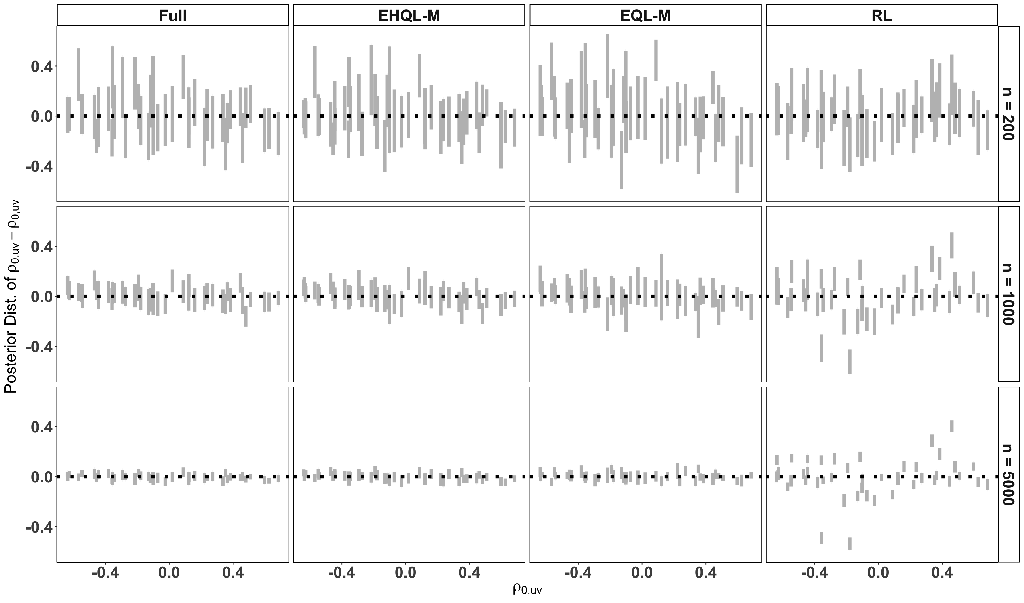
Figure 3: Plots of $95\%$ credible intervals for $\rho_{0,uv}-\rho_{\boldsymbol{\theta},uv}$ for all unique correlations in $\boldsymbol{C}_{0}$ using various $\mathcal{A}$ for three sample sizes. “Full” uses full marginals; “EQL-M” uses the lower/upper bounds and median; “EHQL-M” augments each $\mathcal{A}_{j}$ for EQL-M with $s_{j}\approx 15$ estimated intermediate quantiles. Results are presented for scenario with $~{}50\%$ missing values for each of $p=5$ study variables. The right-most column provides results for the copula correlation estimated under the RL. For the larger sample sizes, posterior inference for $\boldsymbol{C}_{\boldsymbol{\theta}}$ under the EQL/EHQL is accurate with minor efficiency losses when incorporating fewer auxiliary quantiles. In contrast, the inferences under RL can be biased.

We run each EQL/EHQL and RL sampler for 10,000 iterations on a 2023 Macbook Pro. When $n=5000$, the EQL/EHQL samplers average around five minutes to complete, whereas the RL sampler takes nearly four hours. Mixing is also facilitated by introducing $\mathcal{A}$, with apparent convergence of the posterior of $\boldsymbol{C}_{\boldsymbol{\theta}}$ after a few hundred samples.

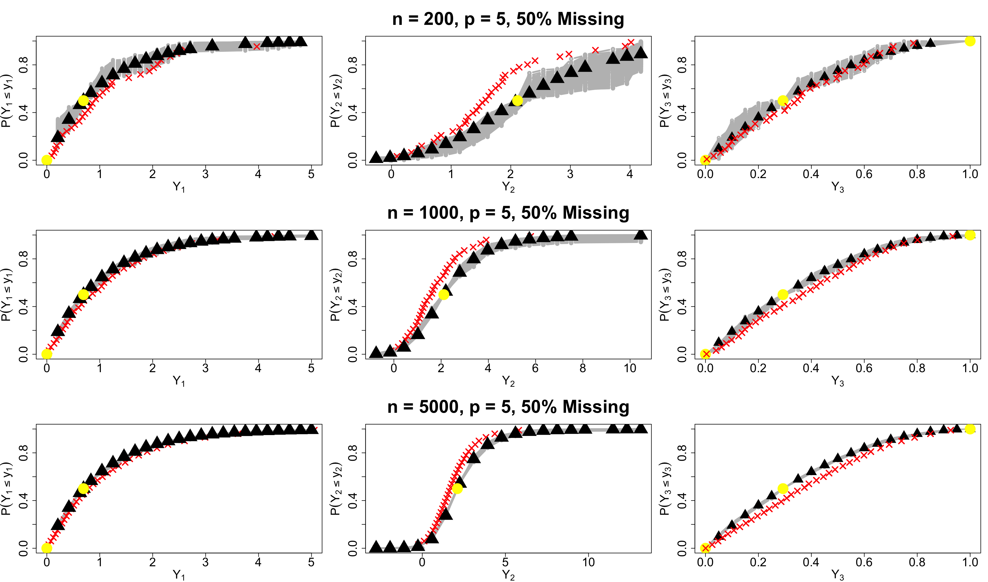
Figure 4: EHQL posterior samples of $\tilde{F}_{j}$ (lines) compared to true $F_{j}(y^{q}_{j})$ (triangles) and empirical CDFs (crosses) computed from $\boldsymbol{y}^{obs}$. Columns index $j=1,2,3$ from left to right. Rows index the sample size. Each $\mathcal{A}^{*}$ uses the lower/upper bounds and the median (dots) and 15 intermediate quantiles. The proposed estimator accurately outlines each true CDF and corrects the biases in the ECDF caused by nonignorable missingness.

Finally, we evaluate how closely (17) under the EHQL-M approximates each true $F_{j}$. Figure 4 displays posterior samples of $\tilde{F}_{j}(y^{q}_{j})$ for $j=1,2,3$ evaluated at the specified intermediate quantile points; it also displays the empirical CDFs (ECDF) computed from $\boldsymbol{y}^{obs}$. These ECDFs exhibit varying degrees of bias caused by the nonignorable missing data. In contrast, each $\tilde{F}_{j}(y^{q}_{j})$ accurately approximates the general shape of $F_{j}$, even though $\mathcal{A}$ only includes bounds and medians. As expected, posterior uncertainty with (17) is highest for regions with relatively small sample sizes.

4.2 Simulation of Repeated Sampling Performance

In this simulation study, we evaluate repeated sampling properties of the EHQL copula with multiple imputation inferences. We use $p=5$ variables from the North Carolina lead exposure data displayed in Table 5, namely Economically Disadvantaged (EconDisadv), Mother’s Age (mAge), Mother’s Race (mRace), an index of Neighborhood Deprivation (NDI), and end-of-fourth grade (EoG) standardized math test scores (Math_Score). These variables are mixed binary, unordered categorical, count, and continuous variables that have complex univariate and multivariate features. We collect all individuals with complete data on these five variables, excluding observations with $\lvert\text{NDI}\rvert>5$ to provide stability, which we treat as a finite population comprising approximately 165,000 individuals. Using this population, we estimate 10th, 50th, and 90th quantile regressions (Koenker, , 2010) of Math_Score on main effects of the other four variables, which we treat as population quantities. The target models aim to uncover potentially heterogeneous effects of the covariates depending on the level of academic achievement, previewing the analysis in Section 5.

We take 500 simple random samples of $n=5000$ individuals from this constructed population. In each sample, we generate nonignorable missingness in NDI. Letting $j=1$ index the variable corresponding to NDI, we do so by the missingness mechanism,

$$p(R_{i1}=1\mid\boldsymbol{y})\sim\mbox{Bernoulli}(\Phi(-0.5-1.3y^{scale}_{i1})),$$ (19)

where superscript ${scale}$ indicates that the variable is centered and scaled to unit variance. After deleting any $y_{i1}$ where $r_{i1}=1$, we have approximately 40% missing values of NDI, with lower values more likely to be missing in the sampled data. We also randomly remove 5% of the other variables, including Math_Score. Because of the nonignorable missingness, complete case analysis could result in biased estimates of the quantile regression coefficients.

As auxiliary information, we assume access to selected quantiles of NDI, which we take from its marginal distribution in the constructed population. Here, we let $\mathcal{A}$ include the lower/upper bounds and median. The supplement includes results using the lower/upper bounds and 75th quantile, which are qualitatively identical to those presented here. We implement the EHQL using 15 evenly spaced quantiles across the range of observed values of NDI. For the other study variables, we use the empirical deciles in the sampled data as the quantiles in $\mathcal{A}$. We add a missingness indicator for NDI to the Gaussian copula model. We exclude the remaining indicators, which effectively models that data for the corresponding variables are MCAR.

We run the Gibbs sampler in Algorithm 1 for 5,000 iterations. After a conservative burn-in of 2,500 draws, we extract interpolated CDFs for imputation using Algorithm 2, and take the completed data in every 125th iteration to create $m=20$ multiple imputations. We estimate the targeted quantile regressions and use the combining rules of Rubin, (1987) for point estimates and 95% confidence intervals for the quantile regression coefficients. We also implement a default application of multiple imputation by chained equations (MICE) based on the mice package in R (van Buuren, , 2018). This does not use $\mathcal{A}$, although we add $R_{1}$ as a predictor for MICE. We repeat the entire procedure of sampling 5000 individuals, making missing values, and obtaining multiple imputation inferences 500 times.

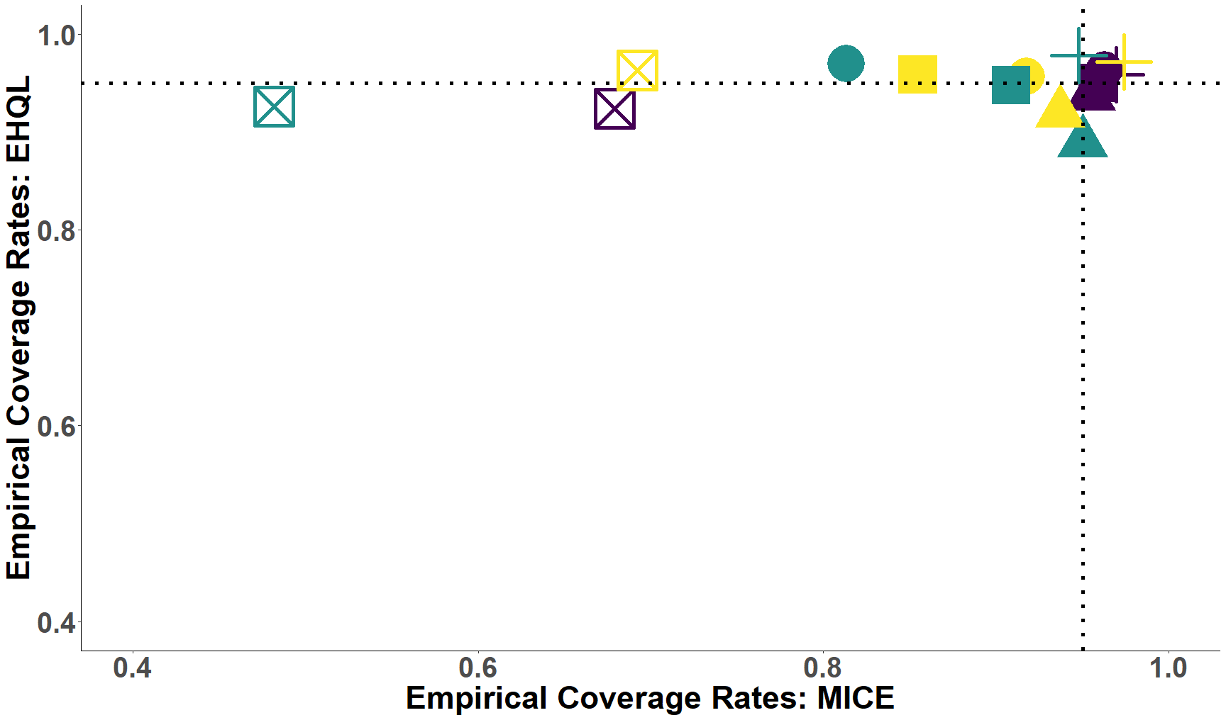
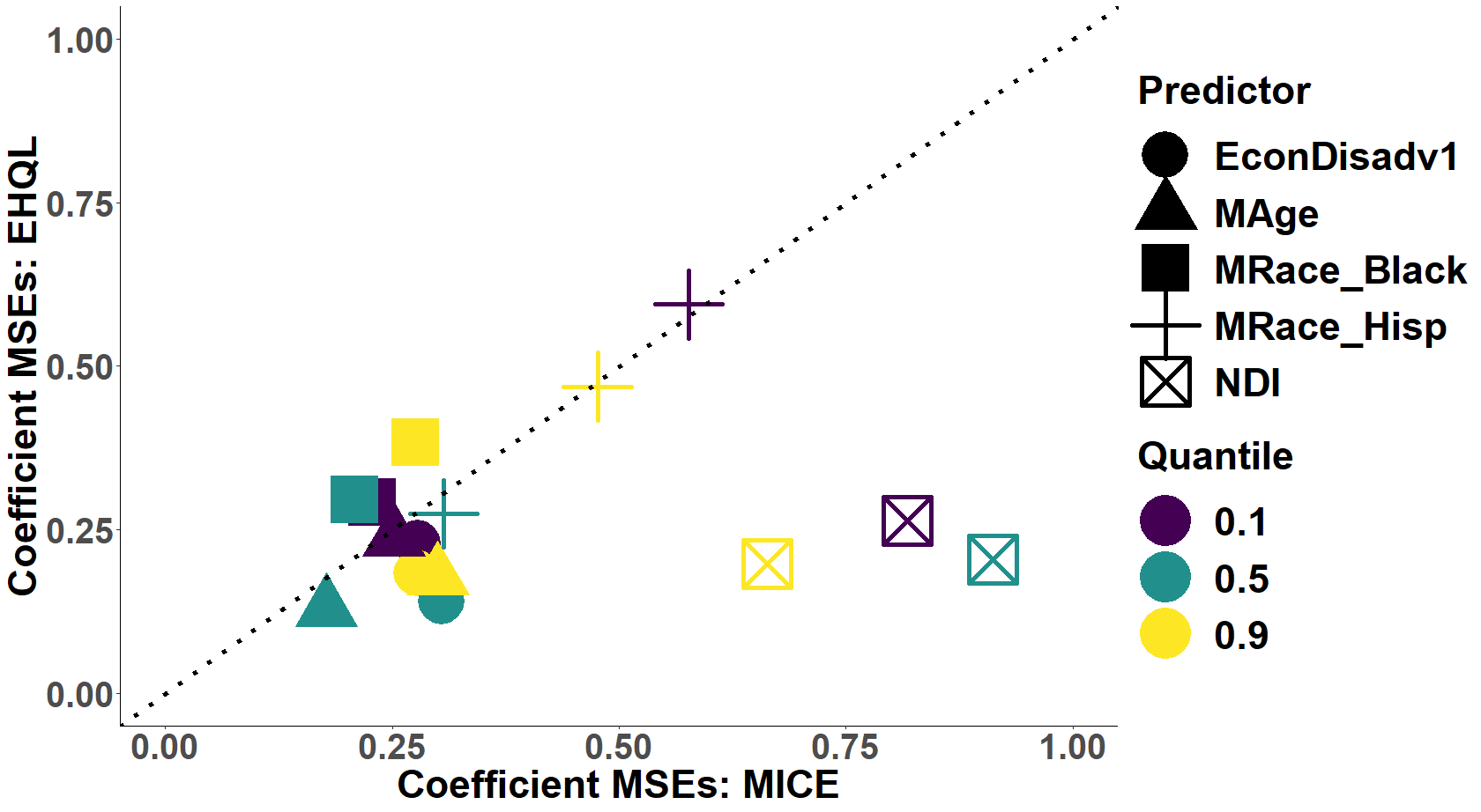
Figure 5: Empirical coverage rates (left) and mean squared error (MSE) of multiple imputation point estimates (right) for the EHQL copula and MICE imputations in the repeated simulation study. For the coefficients of NDI, the EHQL provides significantly lower bias and higher coverage rates. While not shown, the average interval widths are similar.

Figure 5 summarizes the multiple imputation inferences over the 500 runs. The inferences for the coefficients subject to MCAR missingness are reasonably similar for EHQL and MICE, and generally of high quality. However, we see substantial differences among EHQL and MICE coefficient estimates for NDI. These coefficients are accurately estimated with close to nominal coverage rates under EHQL, but not MICE. Evidently, the incorporation of $\mathcal{A}$ and the flexible dependence structure under the copula model allow the imputations to reflect the multivariate relationships more accurately than MICE does. The advantage of EHQL relative to MICE is also evident in the imputations of NDI, which match the population marginal for EHQL but do not for MICE. This is visualized in Figure 6.

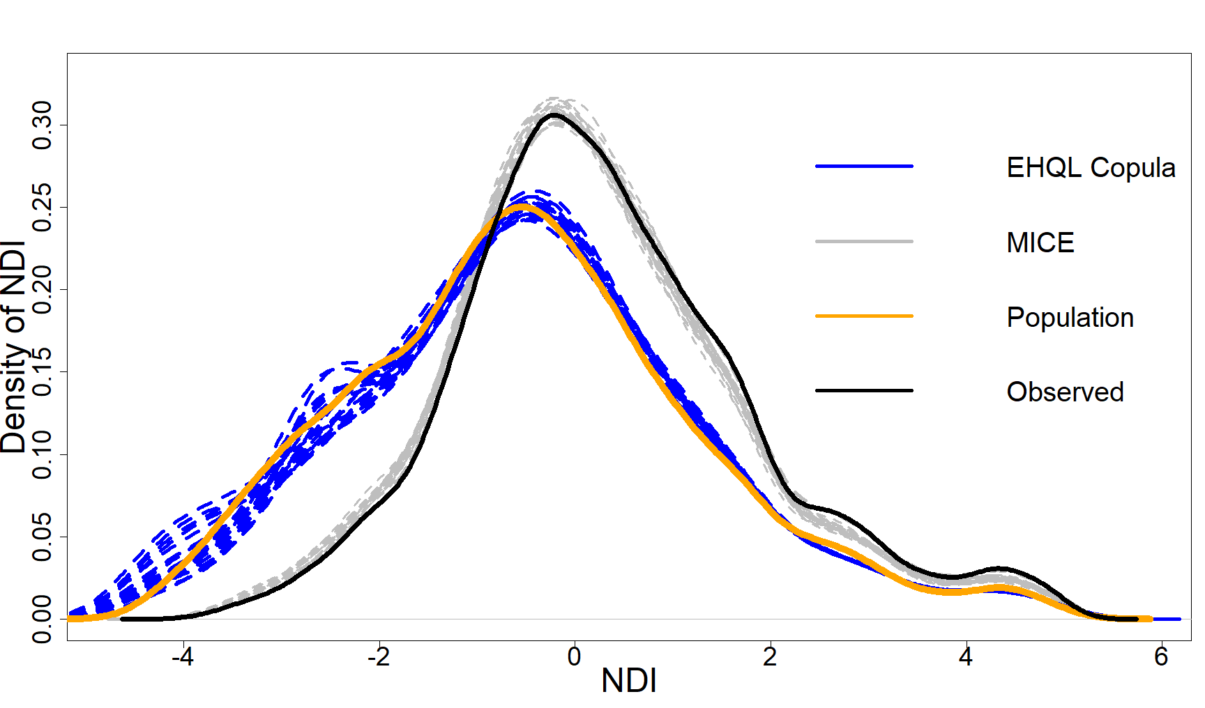
Figure 6: Marginal distribution of NDI in 20 completed datasets produced by EHQL and MICE. The EHQL imputations capture the bi-modality and skewness of the population marginal, whereas the MICE imputations mimic the distribution of the observed values.

5 Analysis of North Carolina Lead Exposure Data

Public health research in recent years has concluded overwhelmingly that lead exposure has adverse impacts on childhood cognitive development (e.g., Bellinger et al., , 1992; Miranda et al., , 2009; Kowal et al., , 2021; Bravo et al., , 2022). Many studies investigating this topic rely on administrative health and education datasets, linked at the individual child level, to estimate associations between lead exposure and outcomes of interest. Typically, blood-lead measurements are available only for children who are tested for lead exposure, and children are more likely to be tested when there is concern about their exposure (Kamai et al., , 2022). Consequently, abundant missingness among lead measurements is commonplace, and individuals who are measured tend to have higher levels of exposure than much of the population. Accurate imputation of lead measurements is important in this setting, as selection biases could influence population-level inferences on the associations between cognitive outcomes and lead exposure (e.g., as simulated in Section 4.2).

Variable Name	$\bar{Y}^{obs}/\bar{Y}^{mis}$	Description
Blood_lead	2.79/NA	Blood lead level (micrograms per deciliter)
Math_Score	448.9/452.5	Standardized score on first 4th grade EoG math test
Reading_Score	445.2/448.5	Standardized score on first 4th grade EoG reading test
mEduc	$(.25,.56,.21)$/ $(.10,.48,.42)\,$	Mother’s education at the time of birth (No degree, High school degree, College degree)
mRace	(.57,.31,.12)/ (.76,.19,.05)	Mother’s race/ethnicity (Non-Hispanic (NH) White, NH Black, Hispanic)
BWTpct	46.9/51.7	Birthweight percentile
mAge	25.9/28.7	Mother’s age at the time of birth
Gestation	38.6/38.7	Gestational period (in weeks)
Male	.50/.50	Male infant (1 = Yes, 0 = No)
Smoker	.15/.09	Mother smoked (1 = Yes, 0 = No)
NotMarried	.46/.22	Not married at time of birth (1 = Yes, 0 = No)
EconDisadv	.61/.32	Economically disadvantaged, per participation in the Child Nutrition Lunch Program (1 = Yes, 0 = No)
RI	.23/.18	Residential isolation index, at time of EoG test
NDI	.10/-1.04	Neighborhood Deprivation Index, at time of EoG test

Table 1: Variables used in the analysis of the relationship between lead exposure and EoG test scores among fourth grade children in North Carolina. Data are restricted to children with 30–42 weeks of gestation, 0–104 weeks of age-within-cohort, mother’s age 15–44, Blood_Lead $\leq$ 10, birth order $\leq$ 4, no status as an English Language Learner, and residence in North Carolina at the time of birth and the time of the EoG test. For the quantile regressions, numeric covariates are scaled to mean 0 with 0.5 standard deviation.

We analyze a dataset containing information on $\sim$170,000 North Carolina children born between 2003 and 2005. The dataset is constructed by linking children’s data across three databases comprising (i) detailed birth records, which include maternal demographics, maternal and infant health measures, and maternal obstetrics history for all documented live births in N.C.; (ii) lead exposure surveillance records from a registry maintained by the state of N.C., which include integer-valued blood-lead levels; and (iii) test score data from the N.C. Education Research Data Center at Duke University, which include EoG reading and mathematics test scores as well as some demographic and socioeconomic information (CEHI, , 2020). Table 1 summarizes the variables we use, including their sample averages among children with lead exposure (Blood_lead) observed or missing. Notably, 35% of the lead measurements are missing. Other variables have missing data rates less than 0.02%.

Figure 7 displays the ECDF of Blood_lead compared to three years of annual point estimates for the 50th, 75th, 90th, and 95th quantiles of lead exposure levels published by the CDC (Centers for Disease Control and Prevention, , 2022). Clearly, the observed distribution does not match the population-level quantile estimates. We therefore consider the missingness in Blood_lead as possibly missing not at random (MNAR). As we discuss later, the EHQL copula correlation estimates suggest this missingness in fact is MNAR.

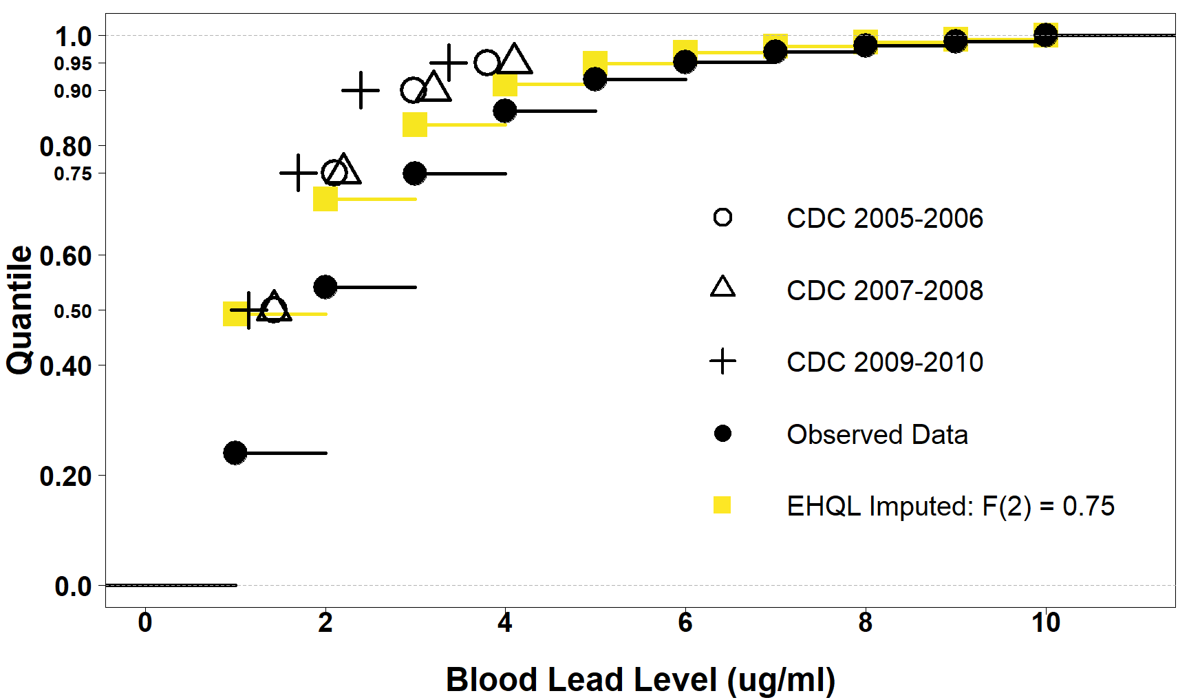
Figure 7: Empirical distribution of Blood_lead in the North Carolina data and population-level quantiles published by the CDC. Also displayed are average estimated quantiles of Blood_lead in completed datasets after EHQL imputations. We include CDC values consistent with the years most children were measured for lead exposure. After imputation, the marginal distribution of Blood_lead more closely matches the population-level estimates.

To adjust for this missingness, we seek to leverage the CDC estimates as auxiliary information for Blood_lead. However, the Blood_lead measurements in the North Carolina data are recorded as integers corresponding to the interval in which the child’s measurement is contained. For instance, Blood_lead=1 means that the child’s measurement was in the interval $(0,1]$ $\mu$g/ml. By contrast, the CDC measurements are continuous. In addition, the CDC estimates are national, which ignores regional or state-specific effects.

We therefore use the CDC estimates to approximately locate the marginal distribution of Blood_lead and employ Algorithm 2 to infer intermediate quantiles. As evident in Figure 7, the 75th quantile estimates from the three years of CDC publications are reliably around 2.0. Because of this stability, we set $\mathcal{A}_{\text{Blood_lead}}=\{F_{\text{Blood_lead}}^{-1}(0)=0,F_{\text{Blood_lead}}^{-1}(0.75)=2,F_{\text{Blood_lead}}^{-1}(1)=10\}$. We also examine sensitivity of results when using $F_{\text{Blood_lead}}^{-1}(0.70)=2$ and $F_{\text{Blood_lead}}^{-1}(0.80)=2$. For the remaining numerical study variables, we use empirical deciles for the auxiliary quantiles. This is reasonable given the scarce missingness and large sample size. These auxiliary quantiles are not varied in the sensitivity analysis.

We use the EHQL copula with the factor model in (18) to implement multiple imputation of all missing values. We include a missingness indicator for Blood_lead but not the other variables, which are almost completely observed. Their indicators comprise almost all zeros and thus are not likely to to inform the imputation but would slow computation. Consequently, the remaining study variables are treated as MCAR. For each set of auxiliary information, we estimate the EHQL copula by running Algorithm 1 for 10,000 iterations and discarding 5,000 draws as burn-in. We use every 250th posterior sample of model parameters to create $m=20$ multiple imputations. Posterior predictive checks suggest that the model reasonably describes the observed data; these are available in the supplement.

Using the completed datasets, we estimate the 10th, 50th, and 90th quantile regressions of math and reading scores on main effects of all the study variables, and derive point estimates and uncertainty quantification using multiple imputation combining rules. These quantities describe potentially heterogeneous impacts of the covariates on low, middle, and high-achieving students, which is of interest to public health research (Miranda et al., , 2009).

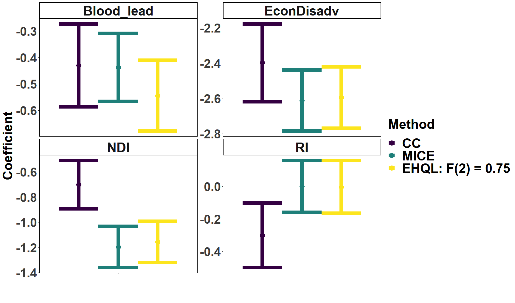
Figure 8: Multiple imputation inferences for coefficients of 10th quantile regression when Blood_lead = 2 is the 75th quantile of the marginal distribution. Compared to complete case analysis, we see sizeable differences especially for the coefficient of Blood_lead. It is estimated to be more adversely associated with EoG math scores. MICE imputations do not capture this difference for Blood_lead, as MICE mimics patterns in the observed data.

Figure 8 summarizes the multiple imputation inferences for the 10th quantile regression coefficients for Blood_lead, EconDisadv, NDI, and RI using Math_Score as the response. The results are presented for $F_{\text{Blood_lead}}^{-1}(0.75)=2$; the findings are insensitive to the other values of this auxiliary quantile. We compare these inferences to those obtained by fitting the quantile regression models to complete case (CC) observations, which exclude any observations with missing study variables, and to results from $m=20$ multiple imputations using a bespoke application of MICE. Results for the other auxiliary quantile specifications, quantile regressions, and using reading scores as the response are in the supplement.

After multiple imputation, we see sizeable shifts in the inferences. The estimated associations of Blood_lead, EconDisadv, and NDI with Math_Score are more adverse than in the CC analysis. The association of Blood_lead with Math_Score is estimated to be significantly stronger when using the EHQL imputations rather than the MICE imputations. Specifically, the point estimate for this coefficient under the EHQL is nearly two standard errors more negative than point estimates under CC and MICE, which is a substantively large change. The inferences under EHQL and MICE are similar for the other predictors’ coefficients, which is not unexpected as these variables have few missing values. Similar shifts are evident in the 50th and 90th quantile regressions as well.

To illuminate the effect of the EHQL imputations further, we examine the empirical CDF of Blood_lead obtained by averaging across the $20$ completed datasets; this is displayed in Figure 7. Because it utilizes $\mathcal{A}$, the EHQL imputes values of missing Blood_lead measurements that are small relative to the observed values. Simultaneously, the percentiles of EoG math scores are higher for students missing Blood_lead than for students with recorded values. Consequently, imputing Blood_lead so that its completed-data distribution accords with $\mathcal{A}$ strengthens its negative association with Math_Score. We see similar strengthening of inverse associations with the other predictors except for RI, which has estimates mostly shrunk towards zero. RI is strongly correlated to NDI, which may help explain why its estimates attenuate. We note that a 95% credible interval for the copula correlation between Blood_lead and its missingness indicator is (-0.92,-0.91), offering additional evidence that the missingness in lead exposure measurements is MNAR.

6 Concluding Remarks

Using auxiliary marginal quantiles offers a convenient and flexible way to handle nonignorable missing data in Gaussian copula models. The simulation studies suggest that using reliable $\mathcal{A}$—for example, informed by external sources like national surveys or administrative databases—can result in more accurate inferences than treating nonignorable missing data as MCAR or MAR. In fact, under AN missingness, it is possible to estimate accurately the copula correlation and perform well-calibrated multiple imputation even with just a few auxiliary quantiles on each study variable. The simulations also suggest that augmenting $\mathcal{A}$ with intermediate quantiles can improve the quality of inferences and imputations.

There are many topics worthy of future research. For example, the marginal quantiles may be known with uncertainty, for example, estimates from a probability sample. In cases where analysts desire a single inference, it may be possible to posit sampling distributions for the true quantiles that can be integrated into the model specification. Additionally, often data have survey weights. While there are methods for using auxiliary margins with survey-weighted data for categorical data models (Akande and Reiter, , 2022; Tang et al., , 2024), work is needed to develop methods for the EQL/EHQL copulas.

The North Carolina lead exposure analysis suggests that utilizing auxiliary marginal quantiles to handle nonignorable missing data can impact empirical findings. In particular, inferences drawn from the multiple imputations based on the EHQL copula suggest that lead exposure affects childhood cognitive development more adversely than might be concluded from a complete case analysis. More broadly, linked data like these are commonly used in public health studies and full of missing values. When the missingness may be MNAR, analysts can consider imputation strategies that leverage known marginal quantiles of the study variables to better inform health policy and intervention strategies.

References

- Akande et al., (2021) Akande, O., Madson, G., Hillygus, D. S., and Reiter, J. P. (2021). Leveraging auxiliary information on marginal distributions in nonignorable models for item and unit nonresponse. Journal of the Royal Statistical Society Series A, 184:643–662.
- Akande and Reiter, (2022) Akande, O. and Reiter, J. P. (2022). Multiple imputations for nonignorable item nonresponse in complex surveys using auxiliary margins. In Statistics in the Public Interest: In Memory of Stephen E. Fienberg, pages 289–306. Cham: Springer.
- Bellinger et al., (1992) Bellinger, D. C., Stiles, K. M., and Needleman, H. L. (1992). Low-level lead exposure, intelligence and academic achievement: a long-term follow-up study. Pediatrics, 90:855–861.
- Bhattacharya and Dunson, (2011) Bhattacharya, A. and Dunson, D. B. (2011). Sparse Bayesian infinite factor models. Biometrika, 98:291–306.
- Bravo et al., (2022) Bravo, M. A., Zephyr, D., Kowal, D., Ensor, K., and Miranda, M. L. (2022). Racial residential segregation shapes the relationship between early childhood lead exposure and fourth-grade standardized test scores. Proceedings of the National Academy of Sciences, 119:e2117868119.
- CEHI, (2020) CEHI (2020). Linked births, lead surveillance, grade 4 end-of-grade scores [data set].
- Centers for Disease Control and Prevention, (2022) Centers for Disease Control and Prevention (2022). CDC Exposure Report Data Tables. https://www.cdc.gov/exposurereport/data_tables.html.
- Chib and Greenberg, (1998) Chib, S. and Greenberg, E. (1998). Analysis of multivariate probit models. Biometrika, 85:347–361.
- Chiba et al., (2015) Chiba, D., Martin, L. W., and Stevenson, R. T. (2015). A copula approach to the problem of selection bias in models of government survival. Political Analysis, 23:42––58.
- Christoffersen et al., (2023) Christoffersen, B., Genz, A., Bretz, F., and Hothorn, T. (2023). mdgc: Missing data imputation using Gaussian copulas. R package version 0.1.7.
- Deng et al., (2013) Deng, Y., Hillygus, D. S., Reiter, J. P., Si, Y., and Zheng, S. (2013). Handling attrition in longitudinal studies: The case for refreshment samples. Statistical Science, 28:238–256.
- Di Lascio et al., (2015) Di Lascio, F., Giannerini, S., and Reale, A. (2015). Exploring copulas for the imputation of complex dependent data. Statistical Methods and Application, 24:159––175.
- Eckert and Hohberger, (2023) Eckert, C. and Hohberger, J. (2023). Addressing endogeneity without instrumental variables: An evaluation of the Gaussian copula approach for management research. Journal of Management, 49:1460–1495.
- Fan and Patton, (2014) Fan, Y. and Patton, A. J. (2014). Copulas in econometrics. Annual Review of Economics, 6:179–200.
- Feldman and Kowal, (2022) Feldman, J. and Kowal, D. R. (2022). Bayesian data synthesis and the utility-risk trade-off for mixed epidemiological data. The Annals of Applied Statistics, 16:2577–2602.
- Feldman and Kowal, (2024) Feldman, J. and Kowal, D. R. (2024). Nonparametric copula models for multivariate, mixed, and missing data. Journal of Machine Learning Research, 25(164):1–50.
- Heitjan and Rubin, (1991) Heitjan, D. F. and Rubin, D. B. (1991). Ignorability and coarse data. The Annals of Statistics, 49:2244–2253.
- Hirano et al., (2001) Hirano, K., Imbens, G. W., Ridder, G., and Rubin, D. B. (2001). Combining panel data sets with attrition and refreshment samples. Econometrica, 69:1645–1659.
- Hoff, (2007) Hoff, P. D. (2007). Extending the rank likelihood for semiparametric copula estimation. The Annals of Applied Statistics, 1:265–283.
- Hoff, (2022) Hoff, P. D. (2022). sbgcop: Semiparametric Bayesian Gaussian copula estimation and imputation. R package version 0.980.
- Hollenbach et al., (2021) Hollenbach, F. M., Bojinov, I., Minhas, S., Metternich, N. W., Ward, M. D., and Volfovsky, A. (2021). Multiple imputation using Gaussian copulas. Sociological Methods & Research, 50:1259–1283.
- Joe, (2014) Joe, H. (2014). Dependence Modeling with Copulas. Chapman & Hall/CRC Press.
- Käärik and Käärik, (2010) Käärik, M. and Käärik, E. (2010). Imputation by Gaussian copula model with an application to incomplete customer satisfaction data. In Lechevallier, Y. and Saporta, G., editors, Proceedings of COMPSTAT’2010, pages 485–492. Physica-Verlag HD.
- Kamai et al., (2022) Kamai, E. M., Daniels, J. L., Delamater, P. L., Lanphear, B. P., MacDonald Gibson, J., and Richardson, D. B. (2022). Patterns of children’s blood lead screening and blood lead levels in North Carolina, 2011–2018 — who is tested, who is missed? Environmental Health Perspectives, 130:067002.
- Koenker, (2010) Koenker, R. (2010). Quantile Regression. Cambridge University Press.
- Kowal et al., (2021) Kowal, D. R., Bravo, M., Leong, H., Bui, A., Griffin, R. J., Ensor, K. B., and Miranda, M. L. (2021). Bayesian variable selection for understanding mixtures in environmental exposures. Statistics in Medicine, 40:4850–4871.
- Linero and Daniels, (2018) Linero, A. R. and Daniels, M. J. (2018). Bayesian approaches for missing not at random outcome data: the role of identifying restrictions. Statistical Science, 33:198–213.
- Miller and Dunson, (2018) Miller, J. W. and Dunson, D. B. (2018). Robust Bayesian inference via coarsening. Journal of the American Statistical Association, 114:1113–1125.
- Miranda et al., (2009) Miranda, M. L., Kim, D., Reiter, J. P., Overstreet Galeano, M. A., and Maxson, P. (2009). Environmental contributors to the achievement gap. Neurotoxicology, 30:1019–1024.
- Molenberghs et al., (2008) Molenberghs, G., Beunckens, C., Sotto, C., and Kenward, M. G. (2008). Every missingness not at random model has a missingness at random counterpart with equal fit. Journal of the Royal Statistical Society, Series B, 70:371–378.
- Murray et al., (2013) Murray, J. S., Dunson, D. B., Carin, L., and Lucas, J. E. (2013). Bayesian Gaussian copula factor models for mixed data. Journal of the American Statistical Association, 108:656–665.
- Pham et al., (2018) Pham, T. M., Carpenter, J. R., Morris, T. P., Wood, A. M., and Petersen, I. (2018). Population-calibrated multiple imputation for a binary/categorical covariate in categorical regression models. Statistics in Medicine, 38:792–808.
- Pitt et al., (2006) Pitt, M., Chan, D., and Kohn, R. (2006). Efficient Bayesian inference for Gaussian copula regression models. Biometrika, 93(3):537–554.
- Rubin, (1976) Rubin, D. B. (1976). Inference and missing data. Biometrika, 63:581––592.
- Rubin, (1987) Rubin, D. B. (1987). Multiple Imputation for Nonresponse in Surveys. New York: John Wiley.
- Sadinle and Reiter, (2017) Sadinle, M. and Reiter, J. P. (2017). Itemwise conditionally independent nonresponse modelling for incomplete multivariate data. Biometrika, 104:207–220.
- Sadinle and Reiter, (2019) Sadinle, M. and Reiter, J. P. (2019). Sequentially additive nonignorable missing data modelling using auxiliary marginal information. Biometrika, 106:889–911.
- Si et al., (2015) Si, Y., Reiter, J. P., and Hillygus, D. S. (2015). Semi-parametric selection models for potentially non-ignorable attrition in panel studies with refreshment samples. Political Analysis, 23:92–112.
- Si et al., (2016) Si, Y., Reiter, J. P., and Hillygus, D. S. (2016). Bayesian latent pattern mixture models for handling attrition in panel studies with refreshment samples. Annals of Applied Statistics, 10:118–143.
- Tang et al., (2024) Tang, J., Hillygus, D. S., and Reiter, J. P. (2024). Using auxiliary marginal distributions in imputations for nonresponse while accounting for survey weights, with application to estimating voter turnout. Journal of Survey Statistics and Methodology, 12:155–182.
- van Buuren, (2018) van Buuren, S. (2018). Flexible Imputation of Missing Data. Chapman & Hall/CRC Press.
- Zhao and Udell, (2020) Zhao, Y. and Udell, M. (2020). Missing value imputation for mixed data via Gaussian copula. In Proceedings of the 26th ACM SIGKDD International Conference on Knowledge Discovery & Data Mining, pages 636–646.