Polarization Wavefront Lidar:
Learning Large Scene Reconstruction from Polarized Wavefronts

Abstract

Lidar has become a cornerstone sensing modality for 3D vision, especially for large outdoor scenarios and autonomous driving. Conventional lidar sensors are capable of providing centimeter-accurate distance information by emitting laser pulses into a scene and measuring the time-of-flight (ToF) of the reflection. However, the polarization of the received light that depends on the surface orientation and material properties is usually not considered. As such, the polarization modality has the potential to improve scene reconstruction beyond distance measurements. In this work, we introduce a novel long-range polarization wavefront lidar sensor (PolLidar) that modulates the polarization of the emitted and received light. Departing from conventional lidar sensors, PolLidar allows access to the raw time-resolved polarimetric wavefronts. We leverage polarimetric wavefronts to estimate normals, distance, and material properties in outdoor scenarios with a novel learned reconstruction method. To train and evaluate the method, we introduce a simulated and real-world long-range dataset with paired raw lidar data, ground truth distance, and normal maps. We find that the proposed method improves normal and distance reconstruction by 53% mean angular error and 41% mean absolute error compared to existing shape-from-polarization (SfP) and ToF methods. Code and data are open-sourced here.

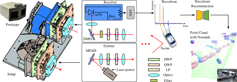
Figure 1: PolLidar sensing and scene reconstruction. We design our PolLidar sensor with a unique capability: it modulates the polarization of light during both the emission and reception stages. To this end, a HWP and QWP are used to emit light of a certain polarization, whereas a QWP and LP are used to determine the polarization of the received light. To capture the received signal, we employ an ADC at the APD for precise raw wavefront measurement. This is unlike traditional Lidar systems that primarily focus on distance measurements and do not provide both the polarization characteristics and the wavefront of the light. Subsequently, a novel lidar geometry reconstruction approach predicting normals, distance and material properties is introduced in Sec. 4.

1 Introduction

Sensing and reconstructing large scenes is crucial for safety-critical applications in autonomous driving [53, 17, 60], drones [33, 45], remote sensing [20, 58], scene understanding [8, 24, 55] and dataset generation [11, 12, 37] for 3D vision. Scanning lidar sensors have been broadly adopted as a cornerstone sensing modality that provides precise distance information. These sensors operate by measuring the ToF of laser pulses emitted into and returned from the scene. The emitted light is typically polarized and the polarization changes upon reflection depending on surface normals and material properties [3, 35]. Off-the-shelf lidar sensors only detect intensity, as such, ignore the additional polarization information. In this paper, we revisit the abandoned geometric and material information in the polarization state for the reconstruction of large automotive scenes up to 100m range.

Although the benefit of polarization has been investigated extensively in other fields [35, 38, 14], polarization is largely unexplored in the context of lidar sensing in vision and robotics. Specifically, lidar and polarization have been explored in meteorology [49, 48, 51], biology [28] and maritime sciences [57] by analyzing the depolarization. Besides, a line of work investigates polarization camera images for shape estimation  [1, 36, 46, 10, 29], stereo depth estimation [54], depth completion [59], and dehazing [5, 50, 21, 56, 22]. These methods have in common that they utilize passive sensors, making them ineffective at night time. Only a few existing works [5, 6] use active polarimetric ToF systems for scene reconstruction. However, these existing time-resolved polarization methods are designed for indoor scenes with object-level contents, prohibiting the measurement of large outdoor scenes.

In this paper, we introduce a novel sensing modality that combines polarization analysis with lidar sensors for scene reconstruction, illustrated in Fig. 1. We devise a polarization wavefront lidar sensor (PolLidar) that is capable of operating in outdoor settings. The proposed sensor modulates the polarization of the emitted and received light. In contrast to polarization cameras, the PolLidar is not limited to a discrete number of polarization states but can measure polarization continuously by finely controlling waveplates and linear polarizers basically able to perform full ellipsometry [13, 25]. The sensor reads the raw wavefront signal directly as a voltage from the Avalanche Photodiode (APD). We employ this sensing technique to capture a polarization dataset consisting of long-range automotive scenes to assess the benefit of polarization. Along with the raw wavefronts, we provide pairwise ground truth distance and normal information from a Velodyne VLS-128 reference sensor, see Fig. 2.

To recover scene properties from polarization wavefront measurements, we combine the proposed sensor with a novel reconstruction approach that operates on the raw polarimetric wavefronts. The proposed reconstruction method uses the polarized wavefronts to estimate surface normals and accurate distance. The estimated normals can then be utilized for predicting material properties, including index of refraction, diffuse and specular albedo, and surface roughness. For training, we extend the CARLA simulator [26] with a realistic polarization model of light to generate a synthetic long-range polarization dataset.

We assess the method with experiments on both synthetic data and real-world data. We find that the proposed method improves distance estimation by 41% mean absolute error compared to conventional ToF methods and 53% mean angular error for normal estimation compared to SfP and point cloud baselines on automotive scenes.

Specifically, we make the following contributions

• We devise a polarization wavefront lidar sensing approach that measures time-resolved polarization properties to recover precise distance and normals for long-range scenarios as found in automotive scenes.

• We propose a neural reconstruction approach for distance and normals operating directly on raw wavefronts instead of post-processed ToF peaks.

• We introduce the first automotive polarization lidar dataset, consisting of real-world data and simulation data. We validate our model with the proposed dataset for long-range distance estimation and dense normal reconstruction. Compared to baseline methods, our model improves distance and normal reconstruction by 41% mean absolute error and 53% mean angular error, respectively.

2 Related Work

Polarization Lidars. Polarization lidar sensors have been explored in diverse fields. Early studies, such as Schotland’s [51], leveraged these polarimetric measurements for cloud property analysis, while approaches as  [51] study the bioaerosols in the atmosphere [28] and in [57] the scattering coefficient of oceans are measured using polarization lidar [57]. Recently, Baek et al. [6, 5] combine a prototypical polarization lidar with a temporal-polarimetric BRDF model to achieve accurate scene reconstruction. Jeon et al. [31] propose a polarimetric indirect ToF imaging method that utilizes polarization to improve depth estimations through scattering media. However, the imaging technique, i.e., the design of the optical path in  [6, 5], and the indirect ToF measurement principle in [31], fundamentally limit these devices to indoor usage. In contrast, the proposed method is the first designed for scene reconstruction in large outdoor scenes up to 100m.

Scene Reconstruction with Passive Polarization Sensors. Exploiting the relationship between the polarization of reflected light and the surface normals, shape from polarization (SfP) methods have achieved scene reconstruction from polarization images captured by linear-polarization cameras [43, 2, 39]. Early SfP methods focus on estimating the surface normal of objects under assumptions of either pure specular reflection [43] or pure diffuse reflection [1, 39]. These methods usually assume an unpolarized light source and suffer from polarization ambiguity issues. Recent works [3, 34, 36, 30] leverage deep learning to solve the ambiguity problem. By training on real-world datasets, the network can better distinguish the ambiguity and mitigate the need for inputting unknown material properties such as refractive index. Baek et al. [4] perform joint optimization of appearance, normals, and refractive index. Deschaintre et al. [16] propose a learning-based inverse learning framework with the front-flash illumination. Dave et al. [15] combine polarization with implicit neural representations to collectively reconstruct the geometry and appearance from multiple images. In general, these reconstruction methods focus on scenes with few objects that are placed to exhibit strong polarization cues with a high degree of polarization (DoP). In outdoor scenes, however, the DoP varies significantly limiting the quality of the reconstruction to high DoP regions. The proposed method allows to exploit the exploitation of polarization cues in both high and low DoP regions.

In [32, 59], passive polarization sensors are combined with other imaging modalities. Kadambi et al. [32] utilize normals from polarization to enhance the details of depth from a Microsoft Kinect sensor. Yoshida et al. [59] use polarization to fill in missing regions in the depth maps. Furthermore, polarization cues are leveraged to augment low-quality depth maps from two-view stereo [62, 23], reciprocal image pairs [18], multi-view stereo [14, 40], or lidars [52]. Recently, Huang et al. [27] and Tian et al. [54] propose stereo polarimetric methods, which utilize two polarization images to solve the ambiguity in SfP. However, as passive sensors are dependent on ambient light, these methods struggle in low-light conditions. The proposed active sensing method allows for accurate reconstructions independently of ambient illumination.

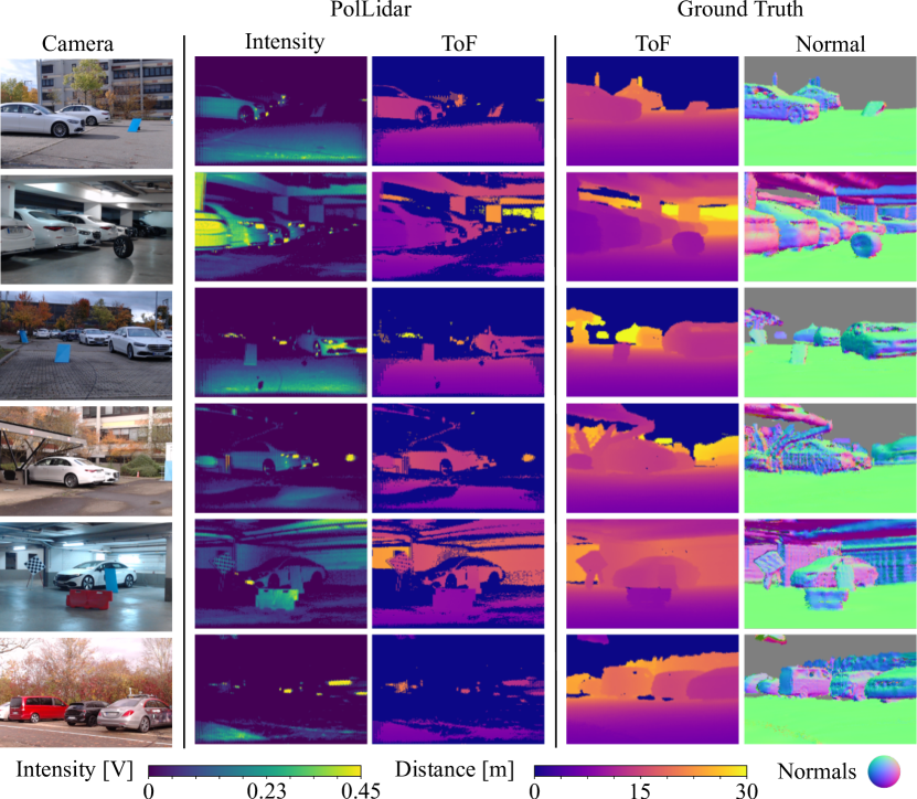
Figure 2: PolLidar dataset. We capture a long-range polarimetric lidar dataset in typical automotive scenes with object distances up to 100m. On the left is a camera reference image, followed by PolLidar intensity for the horizontally polarized state $\theta_{1}^{\{1,2,3,4\}}=0$ and sensor-derived ToF distances. On the right, ground truth data from accumulated scans from a Velodyne VLS-128 lidar, providing ToF and surface normals for comparison.

3 Polarimetric Wavefront Lidar

Figure 3: PolLidar forward model and simulator. Temporal polarimetric reflectance of the scene can be modeled as the sum of specular $\mathbf{M}_{s}$ and diffuse $\mathbf{M}_{d}$ reflection. Receiver and emitter of the PolLidar can be described with the Mueller matrices $\mathbf{P}_{i}$ and $\mathbf{A}_{i}$ that are functions of the rotation angles $\theta_{i}^{\{1,2,3,4\}}$ of HWP, QWPs and LP, respectively. We employ the resulting PolLidar forward model in a simulator based on CARLA that generates synthetic polarimetric raw wavefronts. To this end, we extract material properties and normals from CARLA and feed them into the forward model. The resulting temporal wavefronts are subsequently downsampled in spatial dimension to model beam divergence and noise is added to simulate APD and ADC.

In environmental science, polarimetric lidars are employed for gathering polarization data over extensive ranges, often spanning several kilometers but with a trade-off in spatial resolution. Contrarily, polarimetric lidars for scene reconstruction usually support high spatial resolution, yet their range is limited to a few meters. The proposed PolLidar sensor in Fig. 1 uniquely bridges these application domains. It is designed to allow for a balanced performance optimal for both long-range capabilities up to 223 m and high spatial resolution of 150 rows and 236 columns over a 23.95° and 31.53° vertical and horizontal field-of-view, making it particularly suitable for autonomous driving applications.

Our sensor differs from the ToF systems described in [6, 5]. Specifically, we propose separate modules for emission and reception instead of a shared optical setup. This separation allows for a larger optical aperture in each module, enhancing optical sensitivity and extending the operational range in outdoor scenarios. Instead of the galvo-mirror used in [5], a MEMS micro-mirror is used in the emitter for scene scanning. The receiver employs a digital micro-mirror device (DMD) following [47] to selectively deflect the returning light towards the photodiode. Using the DMD allows for apertures ($\diameter$0.55”) comparable to galvo-mirrors effectively reducing light loss.

To make outdoor applications possible, we operate at a wavelength of 1064 nm and added a narrow bandpass filter, leaving the visible band targeted by existing work. These modifications are essential to suppress ambient light and render the emitted light invisible to the human eye, aligning with automotive illumination standards. The maximum power output adheres to Class-1 eye safety regulations. The laser power remains adjustable according to scenario requirements, offering a balance between achieving maximum range and minimizing saturation which offers a level of control typically not available in off-the-shelf lidars.

On the emission side, the horizontally polarized laser light undergoes modulation by passing through both a half (HWP) and quarter-wave plate (QWP). The receiving module is designed to capture changes in polarization, facilitated by a sequence of a QWP, a linear polarizer (LP), and a bandpass filter, as illustrated in Fig. 1. The rotation of each polarization element is finely adjustable in increments of 0.01 degrees. We use a back-side illuminated Avalanche Photodiode (APD) with an adjustable bias for sensitivity adjustments and read the raw signal with an attached PCIe-5764 FlexRIO-Digitizer analog-to-digital converter (ADC), sampling at 1 Gs/s. This allows us to measure raw wavefronts with a length of 1488 bins of 1 ns width, i.e., 15 cm per bin, and a range of 223 meters.

Our prototype design is optimized for a highly configurable selection of polarization states by finely controlling the polarization elements at the expense of measurement time. The acquisition of a frame, as described in Sec. 4.1, results in a capture time of 5 min. We refer to the Supplementary Material for an analysis on how future setups can achieve real-time capability. Although adding polarization requires additional complexity, we argue that the potential benefits extend beyond the scope of this paper, aiding reconstruction in scenarios with multi-path reflections or scattering media [5].

3.1 Polarimetric Lidar Forward Model

We model polarization with the Stokes-Mueller formalism, with light and reflectance described by a Stokes vector $\mathbf{s}\in\mathbb{R}^{4\times 1}$ and a Mueller matrix $\mathbf{M}\in\mathbb{R}^{4\times 4}$. [13, 7]. Recently, Baek et al. [6] introduced a temporal-polarimetric reflectance model $\mathbf{M}(\tau,\boldsymbol{\omega}_{i},\boldsymbol{\omega}_{o})$ describing how light polarization and intensity change when impinging on a surface with given incident and outgoing direction of light ($\boldsymbol{\omega}_{i}$ and $\boldsymbol{\omega}_{o}$), and with temporal delay ($\tau$) of diffuse reflection. As shown in Fig. 3, the reflectance $\mathbf{M}$ can be modeled as a sum of specular and diffuse reflection ($\mathbf{M}_{s}$ and $\mathbf{M}_{d}$)

$$\mathbf{M}\left(\tau,\boldsymbol{\omega}_{i},\boldsymbol{\omega}_{o}\right) =\mathbf{M}_{s}(\tau,\boldsymbol{\omega}_{i},\boldsymbol{\omega}_{o})+\mathbf{M}_{d}(\tau,\boldsymbol{\omega}_{i},\boldsymbol{\omega}_{o})$$ (1)

$$\mathbf{M}_{s}\left(\tau,\boldsymbol{\omega}_{i},\boldsymbol{\omega}_{o}\right) =\frac{D(\theta_{h};m)G(\theta_{i},\theta_{o};m)}{4\cos\theta_{i}\cos\theta_{o}}\mathbf{D}^{s}(\tau)\mathbf{F}_{R}$$ (2)

$$\mathbf{M}_{d}\left(\tau,\boldsymbol{\omega}_{i},\boldsymbol{\omega}_{o}\right) =\mathbf{C}_{\mathrm{n}\rightarrow\mathrm{o}}\mathbf{F}_{T}^{o}\mathbf{D}^{d}(\tau)\mathbf{F}_{T}^{i}\mathbf{C}_{\mathrm{i}\rightarrow\mathrm{n}},$$ (3)

where $\theta_{h}=\cos^{-1}(\mathbf{h}\cdot\mathbf{n})$, $\theta_{i}=\cos^{-1}(\mathbf{n}\cdot\boldsymbol{\omega}_{i})$, $\theta_{o}=\cos^{-1}(\mathbf{n}\cdot\boldsymbol{\omega}_{o})$ and $\mathbf{n}$ is the surface normal. $D$ and $G$ are functions to describe the surface, where $m$ is the roughness. $\mathbf{C}_{\mathrm{i}\rightarrow\mathrm{n}}$ and $\mathbf{C}_{\mathrm{n}\rightarrow\mathrm{o}}$ are the coordinate-conversion Mueller matrices [13], and $\mathbf{F}_{T}^{i}$, $\mathbf{F}_{T}^{o}$ are the Fresnel transmission Mueller matrices for incident and outgoing light, depending on refractive index $\eta$. $\mathbf{D}^{s}$ and $\mathbf{D}^{d}$ are the depolarization Mueller matrices for specular and diffuse reflections  [6].

Given its long-range working distance, we can assume that the incident and outgoing direction of light in our sensor are identical, and we approximate the reflectance model (1) with a single viewing direction $\boldsymbol{\omega}=\boldsymbol{\omega}_{i}=\boldsymbol{\omega}_{o}$. After scaling $\mathbf{M}$ by the cosine shading term $\cos\phi$ and attenuation such that $\mathbf{H}\left(\tau,\boldsymbol{\omega},\boldsymbol{\omega}\right)=\left(\cos\phi\mathbin{/}d^{2}\right)\mathbf{M}\left(\tau,\boldsymbol{\omega},\boldsymbol{\omega}\right)$, the lidar forward model can be written as

$$I(t,\boldsymbol{\omega}) =\left[\int_{0}^{t^{\prime}}\mathbf{H}(\tau,\boldsymbol{\omega},\boldsymbol{\omega})\mathbf{s}_{\textrm{laser}}(\boldsymbol{\omega},t^{\prime}-\tau)\mathrm{d}\tau\right]_{0},$$ (4)

where $t^{\prime}=t-2d/c$, $d$ is the distance between laser and scene, and $c$ is the speed of light. $\mathbf{s}_{\textrm{laser}}$ denotes the Stokes vector of the emitted laser light. The operator $\left[...\right]_{0}$ denotes taking the first element of the resulting vector.

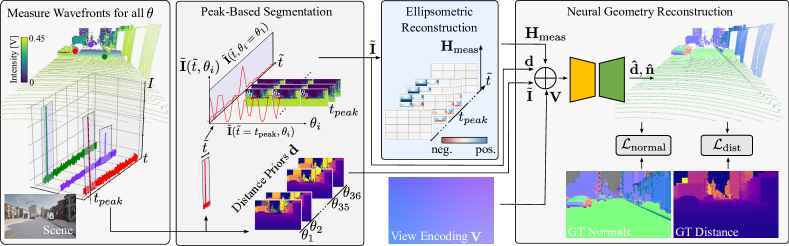
Figure 4: Neural polarization wavefront lidar reconstruction. We capture raw polarization wavefronts of the scene $\mathbf{I}$. We apply a peak-based segmentation technique to obtain a sliced polarization wavefront $\tilde{\mathbf{I}}$ and distance priors $\mathbf{d}$. Via ellipsometric reconstruction, we estimate a sliced Mueller matrix $\mathbf{H}_{\mathrm{meas}}$. Finally, we concatenate all the polarization priors with viewing direction $\mathbf{V}$ as the input to a neural network predicting distance and normals for the scene. We supervised the network with a normal loss $\mathcal{L}_{\mathrm{normal}}$ and a distance loss $\mathcal{L}_{\mathrm{dist}}$.

We use rotating ellipsometry to infer all elements of the Stokes vectors [13]. As illustrated by Fig. 3, a HWP and a QWP are rotated to modulate the polarization of the emitted light. Analogous on the receiving side, a QWP and a LP are used to measure light with a specific polarization incident on the APD. Hence, the image formation of the PolLidar can be modelled as

$$I_{i}(t,\boldsymbol{\omega})=\left[\mathbf{A}_{i}\mathbf{H}(t^{\prime},\boldsymbol{\omega})\mathbf{P}_{i}\mathbf{s}_{\textrm{laser}}(\boldsymbol{\omega},0)\right]_{0},$$ (5)

where $\mathbf{A}_{i}$ and $\mathbf{P}_{i}$ are the $i$-th Mueller matrices of the analyzing optics and the polarizing optics defined as $\mathbf{A}_{i}=\mathbf{L}(\theta_{i}^{4})\mathbf{Q}(\theta_{i}^{3})$ and $\mathbf{P}_{i}=\mathbf{Q}(\theta_{i}^{2})\mathbf{W}(\theta_{i}^{1}),$ with $\theta_{i}^{\{1,2,3,4\}}$ as the rotation angles of the emitter HWP and QWP and the receiver QWP and LP, respectively. $\mathbf{W}$, $\mathbf{Q}$, and $\mathbf{L}$ are the Mueller matrices of the HWP, QWP, and LP [13]. The integral is omitted as a result of using pulsed laser illumination.

3.2 Polarimetric Lidar Simulator

In order to use the PolLidar in a learning-based framework, a sufficient amount of training data is required. However, the finely controllable polarization elements come at the cost of longer measurement times as the motors move relatively slow. To acquire a large polarization wavefront dataset, we integrate the lidar forward model from Eq. (5) into the CARLA simulator [19] to generate vast amounts of synthetic training data. Specifically, we extend the full wavefront lidar model for CARLA as introduced by [26]. As presented in Fig. 3, we extract the material properties $m$, $\mathbf{D}^{s}$ and $\mathbf{D}^{d}$ using custom material cameras. However, materials in CARLA do not have refractive indices $\mu$ assigned by default. We circumvent this problem by extending the ray-tracer to return the material ID of each hit point. Based on the material ID, we look-up the corresponding refractive index $\mu$ in a database [42]. Additionally, we extend the ray-tracer to return normals $\mathbf{n}$ for each hit point.

With material properties and normals in hand, we simulate the scene using the polarimetric lidar forward model. To model the beam divergence of the laser beam, we downsample neighboring rays to eventually render the temporally resolved polarimetric raw wavefronts. Next, we model shot and read-out noise by applying Poisson and Gaussian noise to the wavefronts, respectively. We tune the noise characteristics such that they closely resemble the real device. Additional details are provided in the Supplementary Material.

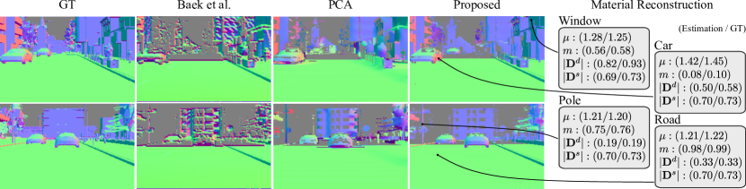
Figure 5: Qualitative evaluation on synthetic data. Baek et al. [6] is unable to reconstruct normals in areas with low DoP, e.g., walls of buildings facing the sensor. PCA [61] applied in this setting are strongly dependent on point cloud density. Thus, distant poles and cars in the second row cannot be reconstructed accurately. The proposed approach leverages polarization cues to reconstruct normals in sparse regions and is robust against low DoP areas. We estimate accurate material properties for different surfaces and objects (right).

4 Neural Polarization Lidar Reconstruction

To leverage polarized raw wavefront data, we devise a learning-based approach for reconstructing normals and distance as presented by Fig. 4. First, we preprocess the wavefronts as described in Sec. 4.1. Next, we train a neural network to predict normals and distance from polarized wavefronts as discussed in Sec. 4.2.

4.1 Preprocessing Wavefronts

When capturing a frame, we perform rotating ellipsometry by collecting raw wavefronts for 36 different rotation angles $\theta_{i}$ subsequently denoted as $\mathbf{I}=\{I_{i}\}_{i=1}^{36}$, where $I_{i}\in\mathbb{R}^{H\times W\times T}$ with $H{=}150$, $W{=}236$ and $T{=}1488$. The temporal resolution $T$ and the repeated measurement for each angle $\theta_{i}$ results in 53,568 samples for each ray in $\mathbf{I}$. To tackle this large dimensional space, we first perform peak-based segmentation to obtain sliced wavefronts as shown in Fig. 4. Specifically, to reduce the temporal dimension, we first locate the peak within the wavefront. Then, we segment a window of size 51 centered around the peak, resulting in a sliced wavefront $\mathbf{\tilde{I}}=\{\tilde{I}_{i}\}_{i=1}^{36}$, where $\tilde{I}_{i}\in\mathbb{R}^{H\times W\times 51}$. We preserve the temporal index of the peak $t_{\mathrm{peak}}$ as it contains the distance information ${\mathbf{d}}\in\mathbb{R}^{36\times H\times W\times 1}$.

As the raw wavefront $\mathbf{\tilde{I}}$ implicitly encodes the polarization optics from emitter and receiver, we apply ellipsometric reconstruction to recover the time-dependent Mueller matrix $\mathbf{H}$. To this end, we use the temporal measurements $I_{i}$ collected at various rotation angles of the polarizing optics to invert the image formation model presented in Eq. (5). Following the approach of Baek et al. [7], we recover the Mueller matrix $\mathbf{H}_{\mathrm{meas}}\in\mathbb{R}^{H\times W\times 51\times 16}$ by solving a least-squares optimization problem as follows

$$\mathop{{\rm{minimize}}}\limits_{\mathbf{H}_{\mathrm{meas}}}\sum_{i=1}^{N}\left(I_{i}-\left[\mathbf{A}_{i}\mathbf{H}_{\mathrm{meas}}\mathbf{P}_{i}\mathbf{s}_{\textrm{laser}}\right]_{0}\right)^{2}.$$ (6)

4.2 Neural Geometry Reconstruction

Subsequent to the pre-processing, we reconstruct the geometry of the scene by inputting the signals to a neural reconstruction network. To this end, the temporal dimension is flattened and the all inputs are concatenated as input $\mathbf{x}$

$$\mathbf{x}=\tilde{\mathbf{I}}\oplus\mathbf{d}\oplus\mathbf{H}_{\mathrm{meas}}\oplus\mathbf{V},$$ (7)

where $\oplus$ denotes concatenation along the feature dimension and $\mathbf{V}$ is the viewing direction. We then predict normals $\hat{\mathbf{n}}$ and distance $\mathbf{\hat{d}}$ with a neural network. The network is a variation of a TransUnet that combines the U-Net and transformer architecture components. Specifically, we use 3 encoder layers to encode the features. At the bottleneck, we use 8 transformer layers. At last, we use 3 decoder layers with skip-connection to predict normals and distance.

To train the network, we supervise normals and distance predictions with a cosine similarity loss for the surface normals and a mean absolute loss for distance

$$\mathcal{L}_{\mathrm{normal}} =|1-(\mathbf{c}\odot\mathbf{n}_{\mathrm{gt}})\cdot(\mathbf{c}\odot\hat{\mathbf{n}}))|_{1},$$ (8)

$$\mathcal{L}_{\mathrm{dist}} =|\mathbf{c}\odot\mathbf{d}_{\mathrm{gt}}-\mathbf{c}\odot\hat{\mathbf{d}})|_{1},$$ (9)

where $\mathbf{c}$ is the confidence mask for the normals where ground truth normals are not available.

We implement the proposed method in PyTorch. We train the model for 200 epochs on a Nvidia A100 GPU. We use the Adam optimizer with a learning rate of 1e-4 and we set the batch size to 1. We crop images to 128×128 patches in each iteration for augmentation. We apply different laser powers and biases during training to increase robustness against saturation and low-intensity readings. More details are presented in the Supplementary Documentation.

Method	Angular Error [°] $\downarrow$			Accuracy [%] $\uparrow$
	Mean	Median	RMSE	$3.0^{\circ}$	$5.0^{\circ}$	$10.0^{\circ}$
SfP-DoP [2]	49.82	35.00	65.39	4.29	7.60	12.63
Baek et al. [6]	31.03	8.32	53.21	27.12	44.44	61.03
PCA [61]	18.64	8.02	33.60	55.89	60.64	66.84
Proposed	8.71	4.31	17.65	65.49	70.19	78.15

Table 1: Quantitative evaluation for normals on synthetic data. The SfP baseline [2] is unable to reconstruct normals in real-world as the underlying assumptions do not translate to real-world scenarios. Baek et al. [6] is designed for object-level ToF imaging and fails in low DoP regions. PCA [61] achieves improved results but with quality depending on point cloud density. The proposed method leverages both the neighborhood of points and the polarization cues; thus outperforming all the baselines.

5 Assessment

To assess the effectiveness of the proposed reconstruction method, we first validate the method on synthetic data with perfect ground truth. Next, we discuss material estimation before validating the method with the experimental device. Finally, we ablate the different inputs to show the benefit of polarized raw wavefronts.

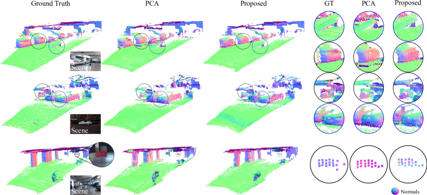
Figure 6: Qualitative evaluation on experimental data. PCA [61] applied on measured captures from our PolLidar results in erroneous predictions of surface normals, especially prominent for the fine structures visible in the zoom-ins of the first two rows, see. e.g., the transition of ground and metal ramp in the first row and the metal roof support in the second row. In contrast, the proposed method is able to resolve these fine details. In the last row, we show a lost cargo scenario with an upright object blocking the road in 50m distance. Our method correctly classifies the object as facing toward the vehicle, whereas PCA predicts a flat surface with downwards oriented normals.

5.1 Synthetic Evaluation

We first validate the proposed neural geometry reconstruction method on synthetic data with perfect ground truth. We compare against three SfP baseline methods to evaluate the quality of the reconstructed normals. Specifically, we evaluate against Baek et al. [6] as a baseline designed for object-level scene reconstruction for a polarimetric ToF prototype. This approach fits the recovered Mueller matrix $\mathbf{H}_{\text{meas}}$ to the polarimetric lidar forward model by jointly estimating material properties and normals. Next, we compare against the classical SfP approach from [2], which recovers surface normals from the DoP by assuming a scene-wide constant refractive index and diffusive reflection. As reported in Tab. 1, classical SfP approaches do not generalize well to outside scenes. This can be attributed to real-world geometry exhibiting regions of high but also very low DoP. Low DoP regions occur when the surface normal and the viewing direction of the lidar align, see Supplementary Dcoumentation. Highlighted by the qualitative findings in Fig. 5, the method from Baek et al. [6] is unable to reconstruct normals in low DoP regions, e.g., buildings of walls that face the sensor, whereas for high DoP regions, as e.g., the side of a vehicle, satisfying performance is achieved.

Moreover, we compare against conventional lidar by averaging wavefronts from all polarization states and applying peak-finding. Treating our PolLidar as conventional makes for an adequate comparison as the number of scanned points is equal for both conventional and PolLidar. Subsequent for normal reconstruction, we apply PCA [61] as a point-cloud based method that considers a neighborhood of points. This method performs well in areas with flat geometry and high point density but degrades significantly at long ranges with sparse distance, e.g., cars in far distances in the second row of Fig. 5 and geometry transition regions, e.g., the area between road and car. PCA also struggles with thin structures like the pole in the second row of Fig. 5. The proposed method leverages the additional polarization cues to resolve normals in regions with sparse points. We also achieve satisfying reconstruction results for regions with weak polarization information by taking a local neighborhood and cues from a normal-dependent widened pulse into account. As a result, the proposed approach outperforms PCA [61] by 53% on the mean angular error as shown in Tab. 1.

For evaluating distance estimation, we compare against the conventional argmax-peak-finding typically performed directly on the device by low-level electronics [9]. This approach is limited by the temporal resolution of the sensor and we find a mean absolute distance error of 32cm. The proposed method leverages the raw wavefront data and the relationship between distance and normals to generate high-quality distance. We find that the proposed method yields a mean absolute distance error of 19cm outperforming the conventional approach by 41% mean absolute error. Additional metrics are provided in the Supplementary Material.

5.2 Material Property Estimation

With estimated surface normals in hand, we reconstruct the material properties, namely index of refraction $\mu$, roughness $m$ and the depolarization matrices $\mathbf{D}^{s}$ and $\mathbf{D}^{d}$, of the polarimetric lidar forward model. To this end, we follow Baek et al. [6] and estimate material properties by rendering the Mueller matrix $\mathbf{H}_{\text{render}}=\mathbf{H}^{s}_{\text{render}}+\mathbf{H}^{d}_{\text{render}}$ that best explains the reconstructed Mueller matrix $\mathbf{H}_{\text{meas}}$. In the large scenes we tackle, we find that the DoP is mostly governed by diffuse reflection. We leverage this heuristic to disentangle the specular and diffusive Mueller matrices. To this end, we solve the following minimization problem

$$\mathop{{\rm{minimize}}}\limits_{\mu,m,|\mathbf{D}^{s}|,|\mathbf{D}^{d}|}{} \lambda^{d}\left|\mathbf{c}_{\text{dop}}\odot(\mathbf{H}_{\text{meas}}-\mathbf{H}^{d}_{\text{render}})\right|_{1}+$$ (10)

$$\lambda^{s}\left|(\mathbf{H}_{\text{meas}}-\mathbf{H}^{d}_{\text{render}})-\mathbf{H}^{s}_{\text{render}}\right|_{1},$$

where $\lambda^{d}$, $\lambda^{s}$ are scalar weights and $\mathbf{c}_{\text{dop}}$ a mask focusing on regions with high diffusive DoP. The weights are chosen such that in the first phase of the minimization, the diffusive loss drives the estimation of the index of refraction $\mu$ which later helps to better disentangle material properties that occur solely in the specular component of the Mueller matrix. Note that in our simulation, only the scalar amplitude, denoted by $|\mathbf{D}^{s}|$ and $|\mathbf{D}^{d}|$, of the depolarization matrices vary and are subsequently optimized for. Fig. 5 validates that the proposed approach is able to successfully recover the material properties of different objects and surfaces. As we do not optimize the surface normals, this further validates the quality of the reconstructed normals as recovering material properties without accurate normals is infeasible.

Method	Angular Error [°] $\downarrow$			Accuracy [%] $\uparrow$
	Mean	Median	RMSE	$3.0^{\circ}$	$5.0^{\circ}$	$10.0^{\circ}$
SfP-DoP [2]	65.92	63.76	70.13	0.02	0.05	0.24
Baek et al. [6]	37.04	13.97	57.25	17.51	27.93	43.36
PCA [61]	18.75	4.86	35.73	41.18	52.87	63.74
Proposed	15.76	4.27	28.73	45.94	55.42	63.80

Table 2: Quantitative evaluation for normals on experimental data. For normal reconstruction with the real device, comparable trends to synthetic data are observable. Due to noisier ground truth and sensor imperfections, the overall error is slightly larger. However, the proposed method recovers accurate normals on real experimental data, outperforming all baseline approaches.

5.3 Experimental Evaluation

Next, we evaluate the proposed approach on real-world data. We pair the PolLidar sensor with a Velodyne VLS-128 reference lidar. Fig. 2 shows PolLidar data with ground truth distance and normals. In total, we capture 60 frames with 3 biases each and scene-adjusted laser power paired with ground-truth distance and normal information. For ground truth, we accumulate point clouds from the reference lidar, generate dense lidar maps, and extract normals from the meshed lidar map.

Fig. 6 reports qualitative reconstruction results. Similar to the synthetic evaluations, PCA [61] introduces artifacts, whereas the proposed approach is able to recover the surface geometry correctly, e.g., the first row of Fig. 6 for the transition area between ground and metal ramp. Furthermore, the proposed approach is able to reconstruct normals in sparse regions, e.g. for the metal support structure of the roof in the second row. These findings are consistent with the quantitative results in Tab. 2, where the proposed approach outperforms the best baseline by 16% mean angular error. For autonomous driving, accurate normals allow us to distinguish obstacles from the road and are crucial for determining if areas of the road can be overridden, e.g., detecting lost-cargo objects on roads [44, 41]. We show such a scenario in the last row of Fig. 6, where normals of a roadblock in 50m distance are predicted correctly as facing towards the vehicle by the proposed approach. In contrast, PCA [61] estimates the roadblock as flat with downward pointing normals likely misclassifying the object as traversable.

For distance estimation, the mean absolute error of conventional argmax-peak-finding amounts to 24 cm, whereas our method yields a mean absolute error of 20 cm outperforming the conventional distance estimation by 17%.

5.4 Ablation Experiments

We further provide an ablation study in Tab. 3. First, the impact of polarization cues is studied. In particular, we remove the polarization information by replacing the raw wavefronts $\mathbf{\tilde{I}}$ with the mean over the different $\theta_{i}$. Removing the polarization cues, increases mean angular error by 22%. Furthermore, we ablate the ellipsometric reconstruction. Specifically, we remove the Mueller matrix from the inputs. As the network needs to learn to disentangle the polarization optics of the emitter and receiver from the scene, the mean angular error of surface normal increases by 12%. Finally, we analyze the impact of using raw wavefronts by setting the window size to 1. Tab. 3 shows that the wavefront carries crucial information for scene reconstruction.

Ablated modules			Mean angular error [∘]
Wavefront	Polarization	Mueller
✓			10.64
✓	✓		9.73
	✓	✓	9.47
✓	✓	✓	8.71

Table 3: Ablation studies for different modules on synthetic data. The quality of the proposed method degrades when the polarization information, Mueller matrix, or wavefront is withheld.

6 Conclusion

This paper introduces a novel long-range polarization wavefront lidar sensor that measures time-resolved polarization-modulated wavefronts. To recover high-resolution scene information from these raw polarimetric wavefronts, we devise a learning-based approach to recover distance, surface normals, and material properties. To train and evaluate the method, we introduce a large synthetic dataset and a real-world long-range dataset with paired raw lidar data, ground truth depth and normal maps. We validate that the proposed method improves normal and depth reconstruction by 53% and 41% in mean angular error and mean absolute distance error compared to existing shape-from-polarization (SfP) and ToF methods. Confirming the potential of the proposed polarimetric wavefront sensing method with a sequential acquisition setup, future work may devise parallelized acquisition setups that capture a subset of polarization states, allowing for real-time polarimetric lidar captures.

Acknowledgements

This work was supported by the AI- SEE project with funding from the FFG, BMBF, and NRC-IRA. Chenyang Lei was supported by the InnoHK program. Seung-Hwan Baek was supported by Korea NRF grant (RS-2023-00211658, 2022R1A6A1A03052954). Felix Heide was supported by an NSF CAREER Award (2047359), a Packard Foundation Fellowship, a Sloan Research Fellowship, a Sony Young Faculty Award, a Project X Innovation Award, and an Amazon Science Research Award.

See pages 1-17 of supplement.pdf

References

- Atkinson [2017] Gary A. Atkinson. Polarisation photometric stereo. Comput. Vis. Image Underst., 160:158–167, 2017.
- Atkinson and Hancock [2006] Gary A. Atkinson and Edwin R. Hancock. Recovery of surface orientation from diffuse polarization. IEEE Trans. Image Process., 15(6):1653–1664, 2006.
- Ba et al. [2020] Yunhao Ba, Alex Gilbert, Franklin Wang, Jinfa Yang, Rui Chen, Yiqin Wang, Lei Yan, Boxin Shi, and Achuta Kadambi. Deep shape from polarization. In ECCV, 2020.
- Baek et al. [2018] Seung-Hwan Baek, Daniel S. Jeon, Xin Tong, and Min H. Kim. Simultaneous acquisition of polarimetric SVBRDF and normals. ACM Trans. Graph., 37(6):268:1–268:15, 2018.
- Baek and Heide [2021] Seung-Hwan Baek and Felix Heide. Polarimetric spatio-temporal light transport probing. ACM Transactions on Graphics (Proc. SIGGRAPH Asia), 40(6), 2021.
- Baek and Heide [2022] Seung-Hwan Baek and Felix Heide. All-photon polarimetric time-of-flight imaging. Proceedings of the IEEE Conference on Computer Vision and Pattern Recognition (CVPR), 2022.
- Baek et al. [2020] Seung-Hwan Baek, Tizian Zeltner, Hyunjin Ku, Inseung Hwang, Xin Tong, Wenzel Jakob, and Min H Kim. Image-based acquisition and modeling of polarimetric reflectance. ACM Trans. Graph., 39(4):139, 2020.
- Behley et al. [2021] Jens Behley, Martin Garbade, Andres Milioto, Jan Quenzel, Sven Behnke, Jürgen Gall, and Cyrill Stachniss. Towards 3d lidar-based semantic scene understanding of 3d point cloud sequences: The semantickitti dataset. The International Journal of Robotics Research, 40(8-9):959–967, 2021.
- Behroozpour et al. [2017] Behnam Behroozpour, Phillip AM Sandborn, Ming C Wu, and Bernhard E Boser. Lidar system architectures and circuits. IEEE Communications Magazine, 55(10):135–142, 2017.
- Berger et al. [2017] Kai Berger, Randolph Voorhies, and Larry H. Matthies. Depth from stereo polarization in specular scenes for urban robotics. In ICRA, 2017.
- Carballo et al. [2020] Alexander Carballo, Jacob Lambert, Abraham Monrroy, David Wong, Patiphon Narksri, Yuki Kitsukawa, Eijiro Takeuchi, Shinpei Kato, and Kazuya Takeda. Libre: The multiple 3d lidar dataset. In 2020 IEEE Intelligent Vehicles Symposium (IV), pages 1094–1101. IEEE, 2020.
- Carlevaris-Bianco et al. [2016] Nicholas Carlevaris-Bianco, Arash K Ushani, and Ryan M Eustice. University of michigan north campus long-term vision and lidar dataset. The International Journal of Robotics Research, 35(9):1023–1035, 2016.
- Collett [2005] Edward Collett. Field guide to polarization. Spie Bellingham, WA, 2005.
- Cui et al. [2017] Zhaopeng Cui, Jinwei Gu, Boxin Shi, Ping Tan, and Jan Kautz. Polarimetric multi-view stereo. In CVPR, 2017.
- Dave et al. [2022] Akshat Dave, Yongyi Zhao, and Ashok Veeraraghavan. Pandora: Polarization-aided neural decomposition of radiance. In European Conference on Computer Vision, pages 538–556. Springer, 2022.
- Deschaintre et al. [2021] Valentin Deschaintre, Yiming Lin, and Abhijeet Ghosh. Deep polarization imaging for 3d shape and svbrdf acquisition. In CVPR, 2021.
- Dewan et al. [2016] Ayush Dewan, Tim Caselitz, Gian Diego Tipaldi, and Wolfram Burgard. Motion-based detection and tracking in 3D LiDAR scans. In IEEE International Conference on Robotics and Automation (ICRA), 2016.
- Ding et al. [2021] Yuqi Ding, Yu Ji, Mingyuan Zhou, Sing Bing Kang, and Jinwei Ye. Polarimetric helmholtz stereopsis. In CVPR, 2021.
- Dosovitskiy et al. [2017] Alexey Dosovitskiy, German Ros, Felipe Codevilla, Antonio Lopez, and Vladlen Koltun. Carla: An open urban driving simulator. In Conference on robot learning, pages 1–16. PMLR, 2017.
- Dubayah and Drake [2000] Ralph O Dubayah and Jason B Drake. Lidar remote sensing for forestry. Journal of forestry, 98(6):44–46, 2000.
- Fang et al. [2014] Shuai Fang, XiuShan Xia, Xing Huo, and ChangWen Chen. Image dehazing using polarization effects of objects and airlight. Optics express, 22(16):19523–19537, 2014.
- Fu et al. [2023] Qiang Fu, Wei Yang, Linlin Si, Meng Zhang, Yue Zhang, Kaiming Luo, Juntong Zhan, and Su Zhang. Study of multispectral polarization imaging in sea fog environment. Frontiers in Physics, 11, 2023.
- Fukao et al. [2021] Yoshiki Fukao, Ryo Kawahara, Shohei Nobuhara, and Ko Nishino. Polarimetric normal stereo. In CVPR, 2021.
- Geiger et al. [2013] Andreas Geiger, Martin Lauer, Christian Wojek, Christoph Stiller, and Raquel Urtasun. 3d traffic scene understanding from movable platforms. IEEE transactions on pattern analysis and machine intelligence, 36(5):1012–1025, 2013.
- Goldstein [2011] Dennis Goldstein. Polarized Light. CRC Press, 3rd edition edition, 2011.
- Goudreault et al. [2023] Felix Goudreault, Dominik Scheuble, Mario Bijelic, Nicolas Robidoux, and Felix Heide. Lidar-in-the-loop hyperparameter optimization. In CVPR, 2023.
- Huang et al. [2023] Tianyu Huang, Haoang Li, Kejing He, Congying Sui, Bin Li, and Yun-Hui Liu. Learning accurate 3d shape based on stereo polarimetric imaging. In Proceedings of the IEEE/CVF Conference on Computer Vision and Pattern Recognition, pages 17287–17296, 2023.
- Huffman et al. [2020] J Alex Huffman, Anne E Perring, Nicole J Savage, Bernard Clot, Benoît Crouzy, Fiona Tummon, Ofir Shoshanim, Brian Damit, Johannes Schneider, Vasanthi Sivaprakasam, et al. Real-time sensing of bioaerosols: Review and current perspectives. Aerosol Science and Technology, 54(5):465–495, 2020.
- Huynh et al. [2010] Cong Phuoc Huynh, Antonio Robles-Kelly, and Edwin R. Hancock. Shape and refractive index recovery from single-view polarisation images. In CVPR, 2010.
- Ikemura et al. [2024] Kei Ikemura, Yiming Huang, Felix Heide, Zhaoxiang Zhang, Qifeng Chen, and Chenyang Lei. Robust depth enhancement via polarization prompt fusion tuning. arXiv preprint arXiv:2404.04318, 2024.
- Jeon et al. [2023] Daniel S Jeon, Andréas Meuleman, Seung-Hwan Baek, and Min H Kim. Polarimetric itof: Measuring high-fidelity depth through scattering media. In Proceedings of the IEEE/CVF Conference on Computer Vision and Pattern Recognition, pages 12353–12362, 2023.
- Kadambi et al. [2015] Achuta Kadambi, Vage Taamazyan, Boxin Shi, and Ramesh Raskar. Polarized 3d: High-quality depth sensing with polarization cues. In ICCV, 2015.
- Kellner et al. [2019] James R Kellner, John Armston, Markus Birrer, KC Cushman, Laura Duncanson, Christoph Eck, Christoph Falleger, Benedikt Imbach, Kamil Král, Martin Krŭček, et al. New opportunities for forest remote sensing through ultra-high-density drone lidar. Surveys in Geophysics, 40:959–977, 2019.
- Kondo et al. [2020] Yuhi Kondo, Taishi Ono, Legong Sun, Yasutaka Hirasawa, and Jun Murayama. Accurate polarimetric BRDF for real polarization scene rendering. In ECCV, 2020.
- Lei et al. [2020] Chenyang Lei, Xuhua Huang, Mengdi Zhang, Qiong Yan, Wenxiu Sun, and Qifeng Chen. Polarized reflection removal with perfect alignment in the wild. In CVPR, 2020.
- Lei et al. [2022] Chenyang Lei, Chenyang Qi, Jiaxin Xie, Na Fan, Vladlen Koltun, and Qifeng Chen. Shape from polarization for complex scenes in the wild. In Proceedings of the IEEE/CVF Conference on Computer Vision and Pattern Recognition, pages 12632–12641, 2022.
- Linnhoff et al. [2022] Clemens Linnhoff, Dominik Scheuble, Mario Bijelic, Lukas Elster, Philipp Rosenberger, Werner Ritter, Dengxin Dai, and Hermann Winner. Simulating road spray effects in automotive lidar sensor models. arXiv preprint arXiv:2212.08558, 2022.
- Lyu et al. [2019] Youwei Lyu, Zhaopeng Cui, Si Li, Marc Pollefeys, and Boxin Shi. Reflection separation using a pair of unpolarized and polarized images. In NeurIPS, 2019.
- Miyazaki et al. [2003] Daisuke Miyazaki, Robby T. Tan, Kenji Hara, and Katsushi Ikeuchi. Polarization-based inverse rendering from a single view. In ICCV, 2003.
- Miyazaki et al. [2016] Daisuke Miyazaki, Takuya Shigetomi, Masashi Baba, Ryo Furukawa, Shinsaku Hiura, and Naoki Asada. Surface normal estimation of black specular objects from multiview polarization images. Optical Engineering, 56(4):041303, 2016.
- Pinggera et al. [2016] Peter Pinggera, Sebastian Ramos, Stefan Gehrig, Uwe Franke, Carsten Rother, and Rudolf Mester. Lost and found: detecting small road hazards for self-driving vehicles. In 2016 IEEE/RSJ International Conference on Intelligent Robots and Systems (IROS), pages 1099–1106. IEEE, 2016.
- [42] Mikhail N. Polyanskiy. Refractive index database. https://refractiveindex.info. Accessed on 2023-11-12.
- Rahmann and Canterakis [2001] Stefan Rahmann and Nikos Canterakis. Reconstruction of specular surfaces using polarization imaging. In CVPR, 2001.
- Ramos et al. [2017] Sebastian Ramos, Stefan Gehrig, Peter Pinggera, Uwe Franke, and Carsten Rother. Detecting unexpected obstacles for self-driving cars: Fusing deep learning and geometric modeling. In 2017 IEEE Intelligent Vehicles Symposium (IV), pages 1025–1032. IEEE, 2017.
- Risbøl and Gustavsen [2018] Ole Risbøl and Lars Gustavsen. Lidar from drones employed for mapping archaeology–potential, benefits and challenges. Archaeological Prospection, 25(4):329–338, 2018.
- Riviere et al. [2017] Jérémy Riviere, Ilya Reshetouski, Luka Filipi, and Abhijeet Ghosh. Polarization imaging reflectometry in the wild. ACM Trans. Graph., 36(6):206:1–206:14, 2017.
- Royo and Gras [United States Patent 9689667B2 2013] Santiago Royo Royo and Jordi Riu Gras. System, method and computer program for receiving a light beam, United States Patent 9689667B2 2013.
- Sassen [1991] Kenneth Sassen. The polarization lidar technique for cloud research: A review and current assessment. Bulletin of the American Meteorological Society, 72(12):1848–1866, 1991.
- Sassen [2005] Kenneth Sassen. Polarization in lidar. In LIDAR: Range-resolved optical remote sensing of the atmosphere, pages 19–42. Springer, 2005.
- Schechner et al. [2001] Yoav Y. Schechner, Srinivasa G. Narasimhan, and Shree K. Nayar. Instant dehazing of images using polarization. In CVPR, 2001.
- Schotland et al. [1971] Richard M Schotland, Kenneth Sassen, and Richard Stone. Observations by lidar of linear depolarization ratios for hydrometeors. Journal of Applied Meteorology and Climatology, 10(5):1011–1017, 1971.
- Shakeri et al. [2021] Moein Shakeri, Shing Yang Loo, Hong Zhang, and Kangkang Hu. Polarimetric monocular dense mapping using relative deep depth prior. IEEE Robotics and Automation Letters, 6(3):4512–4519, 2021.
- Shi et al. [2020] Shaoshuai Shi, Chaoxu Guo, Li Jiang, Zhe Wang, Jianping Shi, Xiaogang Wang, and Hongsheng Li. PV-RCNN: Point-voxel feature set abstraction for 3D object detection. In IEEE/CVF Conference on Computer Vision and Pattern Recognition (CVPR), 2020.
- Tian et al. [2023] Chaoran Tian, Weihong Pan, Zimo Wang, Mao Mao, Guofeng Zhang, Hujun Bao, Ping Tan, and Zhaopeng Cui. Dps-net: Deep polarimetric stereo depth estimation. In Proceedings of the IEEE/CVF International Conference on Computer Vision, pages 3569–3579, 2023.
- Tian et al. [2021] Shishun Tian, Minghuo Zheng, Wenbin Zou, Xia Li, and Lu Zhang. Dynamic crosswalk scene understanding for the visually impaired. IEEE transactions on neural systems and rehabilitation engineering, 29:1478–1486, 2021.
- Treibitz and Schechner [2009] Tali Treibitz and Yoav Y. Schechner. Active polarization descattering. IEEE Trans. Pattern Anal. Mach. Intell., 31(3):385–399, 2009.
- Vasilkov et al. [2001] Alexander P Vasilkov, Yury A Goldin, Boris A Gureev, Frank E Hoge, Robert N Swift, and C Wayne Wright. Airborne polarized lidar detection of scattering layers in the ocean. Applied Optics, 40(24):4353–4364, 2001.
- Weitkamp [2006] Claus Weitkamp. Lidar: range-resolved optical remote sensing of the atmosphere. Springer Science & Business, 2006.
- Yoshida et al. [2018] Tomonari Yoshida, Vladislav Golyanik, Oliver Wasenmüller, and Didier Stricker. Improving time-of-flight sensor for specular surfaces with shape from polarization. In 2018 25th IEEE International Conference on Image Processing (ICIP), pages 1558–1562. IEEE, 2018.
- Zhang and Singh [2014] Ji Zhang and Sanjiv Singh. LOAM : LiDAR odometry and mapping in real-time. Robotics: Science and Systems Conference (RSS), 2014.
- Zhou et al. [2018] Qian-Yi Zhou, Jaesik Park, and Vladlen Koltun. Open3D: A modern library for 3D data processing. CoRR, abs/1801.09847, 2018.
- Zhu and Smith [2019] Dizhong Zhu and William A. P. Smith. Depth from a polarisation + RGB stereo pair. In CVPR, 2019.