Recurrent neural chemical reaction networks that

approximate arbitrary dynamics

Alexander Dack^,   Benjamin Qureshi   Thomas E. Ouldridge   Tomislav Plesa^,

Keywords: Chemical Reaction Networks;   Dynamical Systems;   Artificial Neural Networks.

Abstract: Many important phenomena in chemistry and biology are realized via dynamical features such as multi-stability, oscillations, and chaos. Construction of novel chemical systems with such finely-tuned dynamics is a challenging problem central to the growing field of synthetic biology. In this paper, we address this problem by putting forward a molecular version of a recurrent artificial neural network, which we call a recurrent neural chemical reaction network (RNCRN). We prove that the RNCRN, with sufficiently many auxiliary chemical species and suitable fast reactions, can be systematically trained to achieve any dynamics. This approximation ability is shown to hold independent of the initial conditions for the auxiliary species, making the RNCRN more experimentally feasible. To demonstrate the results, we present a number of relatively simple RNCRNs trained to display a variety of biologically-important dynamical features.

1 Introduction

Artificial neural networks (ANNs) are a set of algorithms, inspired by the structure and function of the brain, which are commonly implemented on electronic machines [1]. ANNs are known for their powerful function approximating abilities [2, 3], and have been successfully applied to solve complex tasks ranging from image classification [4] to dynamical control of chaos [5]. Given the success of ANNs on electronic machines, it is unsurprising that there has been substantial interest in mapping common ANNs to chemical reaction networks (CRNs) [6, 7, 8, 9, 10, 11, 12, 13, 14, 15] - a mathematical framework used for modelling chemical and biological processes. In this paper, we say that a CRN is neural if it executes an ANN algorithm. Neural CRNs have been implemented experimentally using a range of molecular substrates[16, 17, 18, 19, 20, 21]. As such, these networks, and other forms of chemically-realized computing systems [22, 23, 24, 25, 26, 27, 28], intend to embed computations inside biochemical systems, where electronic machines cannot readily operate.

Current literature on neural CRNs has focused on solving static problems, where the goal is to take an input set of chemical concentrations and produce a time-independent (static) output. These static neural CRNs find application as classifiers [29, 30] in symbol and image recognition tasks [10, 31, 32, 12], complex logic gates [11, 20], and disease diagnostics [17]. However, more intricate time-dependent (dynamical) features can be of great importance in biology. In particular, under suitable conditions, many biological processes can be modelled dynamically using ordinary-differential equations (ODEs). In this context, fundamental processes such as cellular differentiation and circadian clocks are realized via ODEs that exhibit features such as coexistence of multiple favourable states (multi-stability) and oscillations [33, 34, 35]. In fact, even deterministic chaos, a complicated dynamical behaviour, is thought to confer a survival advantage to populations of cells [35].

Despite their promising potential in biology, neural CRNs trained to emulate such dynamical behaviours remain largely unexplored in the literature. To bridge the gap, in this paper we present a novel neural CRN called the recurrent neural chemical reaction networks (RNCRNs) (see Figure 1). We prove that RNCRNs can approximate the dynamics of any well-behaved target system of ODEs, provided that there are sufficiently many auxiliary chemical species and that these species react sufficiently fast. A major advantage of RNCRNs over some other comparable methods for designing chemical systems [36, 37] is that the initial concentrations for the auxiliary species are not constrained. This fact is important, since high-precision experimental fine-tuning of initial concentrations is infeasible [38].

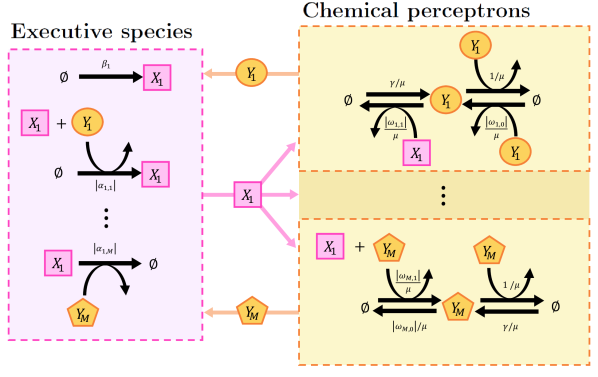
Figure 1: A visualisation of an RNCRN with an executive species $X_{1}$, and a layer of chemical perceptrons $Y_{1},\dots,Y_{N}$. Chemical reactions, as defined in Section 2.1, are shown by horizontal black arrows. The curved black arrows show catalytic involvement of additional chemical species in a chemical reaction. The purple and orange arrows emphasise the interdependence of the executive species and the chemical perceptrons. The absolute value is used to emphasise that all reactions have positive rate constants; where an RNCRN parameter is required to be negative, this is achieved by using a degradation/inactivation reaction as opposed to a production/activation reaction. The explicit CRN is stated in Appendix A.

The paper is organized as follows. In Section 2, we present some background theory on CRNs and ANNs. In Section 3, we introduce an RNCRN, and outline the main theoretical result regarding its approximation properties; this result is stated rigorously and proved in Appendix A. A generalised RNCRN is presented in Appendix B. In Section 4, we present an algorithm for training the RNCRN as Algorithm 1, which we demonstrate by obtaining relatively simple RNCRNs displaying multi-stability, oscillations and chaos; more details can be found in Appendix C. Finally, we provide a summary and discussion in Section 5.

2 Background theory

In this section, we present some background theory on chemical reaction networks and artificial neural networks.

2.1 Chemical reaction networks (CRNs)

Consider two chemical species $X$ and $Y$ which interact via the following five reactions:

$$X+Y \xrightarrow[]{\alpha}Y,\;\;\;\;\varnothing\xrightarrow[]{\beta}X,\;\;\;\;\varnothing\xrightarrow[]{\gamma}Y,\;\;\;\;X+Y\xrightarrow[]{\omega}X+2Y,\;\;\;\;2Y\xrightarrow[]{1}Y.$$ (1)

In particular, according to the first reaction, when species $X$ and $Y$ react, one molecule of $X$ is degraded. Since the molecular count of $Y$ remains unchanged when this reaction occurs, we say that $Y$ acts as a catalyst for the first reaction. The second reaction describes a production of $X$ from some chemical species which we do not explicitly model, and simply denote by $\varnothing$; similarly, the third reaction describes production of $Y$. One molecule of $Y$ is produced when $X$ and $Y$ react according to the fourth reaction. In this reaction, $X$ remains unchanged, and is therefore a catalyst. Finally, according to the fifth reaction, when two molecules of $Y$ react, one of the molecules is degraded. Systems of chemical reactions, such as (1), are called chemical reaction networks (CRNs) [39].

Reaction-rate equations. In this paper, we make a standard assumption on the rate at which the reactions occur: it given by the product of the concentrations of the underlying reactants (species on the left-hand side of the reaction) multiplied by the rate coefficient - the positive number displayed above the reaction arrow. This choice of rates is called the mass-action kinetics. For example, let us denote the concentrations of $X$ and $Y$ from (1) at time $t\geq 0$ respectively by $x=x(t)$ and $y=y(t)$. The first reaction from (1) has $\alpha>0$ as its rate coefficient, and thus occurs at the rate $\alpha xy$. Similarly, the rates of the other four reactions from (1) are given by $\beta$, $\gamma$, $\omega xy$ and $y^{2}$; note that for the final reaction, we have fixed the rate coefficient to $1$. Under suitable conditions [39], the concentrations of chemical species satisfy a system of ordinary-differential equations (ODEs) called the reaction-rate equations (RREs). For system (1), the RREs are given by

$$\frac{\mathrm{d}x}{\mathrm{d}t} =\beta-\alpha xy,\;\;\;\;\;\;\frac{\mathrm{d}y}{\mathrm{d}t}=\gamma+\omega xy-y^{2}.$$ (2)

In what follows, we denote the chemical species by $X_{1},X_{2},\ldots,Y_{1},Y_{2},\ldots$, their corresponding concentrations by $x_{1},x_{2},\ldots,y_{1},y_{2},\ldots\geq 0$, and the rate coefficients of the underlying reactions using the Greek letters $\alpha,\beta,\gamma,\omega>0$ with appropriate subscript indices. For simplicity, we assume that all the variables, including the rate coefficients, are dimensionless. Furthermore, we limit ourselves to the chemical reactions with at most two reactants. In this case, the RREs have quadratic polynomials on the right-hand side, as in (2). More general chemical reactions, with three or more reactants, are experimentally unlikely to occur, and can be approximately reduced to reactions with at most two reactants [40, 41].

2.2 Artificial neural networks (ANNs)

Artificial neural networks (ANNs) consist of connected processing units known as artificial neurons. In this paper, we consider a particular type of artificial neurons called the perceptron [42]. Given a set of inputs, a perceptron first applies an affine function, followed by a suitable non-linear function, called the activation function, to produce a single output. More precisely, let $x_{1},x_{2},\ldots,x_{N}\in\mathbb{R}$ be the input values, $\omega_{1},\omega_{2},\ldots,\omega_{N}\in\mathbb{R}$ be the weights, $\omega_{0}\in\mathbb{R}$ a bias, and $\sigma:\mathbb{R}\to\mathbb{R}$ a suitable non-linear function. Then, the perceptron is a function $y:\mathbb{R}^{N}\to\mathbb{R}$ defined as

$$y=y(x_{1},\ldots,x_{N}) =\sigma\left(\sum_{j=1}^{N}\omega_{j}x_{j}+\omega_{0}\right).$$ (3)

Chemical perceptron. A natural question arises: Is there a CRN with single species $Y$ such that its RRE has a unique stable equilibrium of the form (3)? Such an RRE has been put forward and analyzed in [14], and takes the following form:

$$\frac{\mathrm{d}y}{\mathrm{d}t} =\gamma+\left(\sum_{j=1}^{N}\omega_{j}x_{j}+\omega_{0}\right)y-y^{2}.$$ (4)

A CRN corresponding to (4) is given by

$$\varnothing \xrightarrow[]{\gamma}Y,\;\;\;\;Y\xrightarrow[]{\left|\sum_{j=1}^{N}\omega_{j}x_{j}+\omega_{0}\right|}Y+sY,\;\;\;\;2Y\xrightarrow[]{1}Y,$$ (5)

where $s=\textrm{sign}(\sum_{j=1}^{N}\omega_{j}x_{j}+\omega_{0})$, with function $\textrm{sign}(\cdot)$ yielding the sign of a real number. We call species $Y$ from (5) a chemical perceptron. Setting the left-hand side in (4) to zero, one finds that there is a unique globally stable non-negative equilibrium, which we denote by $y^{*}$, given by

$$y^{*} =\sigma_{\gamma}\left(\sum_{j=1}^{N}\omega_{j}x_{j}+\omega_{0}\right)\equiv\frac{1}{2}\left[\left(\sum_{j=1}^{N}\omega_{j}x_{j}+\omega_{0}\right)+\sqrt{\left(\sum_{j=1}^{N}\omega_{j}x_{j}+\omega_{0}\right)^{2}+4\gamma}\right].$$ (6)

We call $\sigma_{\gamma}$ with $\gamma>0$ a chemical activation function. As $\gamma\to 0$, $\sigma_{\gamma}$ approaches the rectified linear unit (ReLU) activation function [14], which is a common choice in the ANN literature [4].

3 Recurrent neural chemical reaction networks (RNCRNs)

Let us consider a target ODE system with initial conditions, given by

$$\frac{\mathrm{d}\bar{x}_{i}}{\mathrm{d}t} =f_{i}(\bar{x}_{1},\ldots,\bar{x}_{N}),\hskip 14.22636pt\bar{x}_{i}(0)=a_{i}\geq 0,\;\;\;\textrm{for }i=1,2,\ldots,N.$$ (7)

In what follows, we call the ODE right-hand side $(f_{1},f_{2},\ldots,f_{N})$ a vector field, which we assume is sufficiently smooth. Without loss of generality, we assume that (7) has desirable dynamical features in the positive orthant $\mathbb{R}_{>}^{N}$. If such features are located elsewhere, a suitable affine change of coordinates can be used to move these features to the positive orthant [43].

We wish to find a neural CRN with some chemical species $X_{1},\dots,X_{N}$ such that the RREs for these species approximate the target ODEs (7). To this end, let us consider the RREs and initial conditions given by

$$\frac{\mathrm{d}x_{i}}{\mathrm{d}t} =\beta_{i}+x_{i}\sum_{j=1}^{M}\alpha_{i,j}y_{j},\hskip 82.51282ptx_{i}(0)=a_{i},\;\;\;\textrm{for }i=1,2,\ldots,N,$$

$$\mu\frac{\mathrm{d}y_{j}}{\mathrm{d}t} =\gamma+y_{j}\left(\sum_{i=1}^{N}\omega_{j,i}x_{i}+\omega_{j,0}\right)-y_{j}^{2},\hskip 14.22636pty_{j}(0)=b_{j},\;\;\;\textrm{for }j=1,2,\ldots,M.$$ (8)

We call the CRN corresponding to the RREs (8) a recurrent neural chemical reaction network (RNCRN). In Figure 1, we schematically display this RNCRN with $N=1$. The RNCRN consists of two sub-networks, the first of which is the executive sub-system, shown in purple in Figure 1, which contains chemical reactions which directly change the executive species $X_{1},X_{2},\ldots,X_{N}$. Note that the initial conditions for the executive species from (8) match the target initial conditions from (7). The second sub-network is called the neural sub-system, shown in yellow in Figure 1, and it contains those reactions which directly influence the auxiliary species $Y_{1},Y_{2},\ldots,Y_{M}$, for which we allow arbitrary initial conditions $b_{1},b_{2},\ldots,b_{M}\geq 0$. These species can be formally identified as chemical perceptrons, see (4)–(5). However, let us stress that the CRN (5) with RRE (4) depends on the parameters $x_{1},x_{2},\ldots,x_{N}$. In contrast, the concentrations of chemical perceptrons from the RNCRN depend on the executive variables $x_{1}(t),x_{2}(t),\ldots,x_{N}(t)$, which in turn depend on the perceptron concentrations $y_{1}(t),y_{2}(t),\ldots,y_{M}(t)$. In other words, there is a feedback between the executive and neural systems, giving the RNCRN a recurrent character. This feedback is catalytic in nature: the chemical perceptrons are catalysts in the executive system; similarly, executive species are catalysts in the neural system.

Main result. We now wish to choose the parameters in the RNCRN so that the concentrations of the executive species $x_{i}(t)$ from (8) are close to the target variables $\bar{x}_{i}(t)$ from (7). Key to achieving this match is the parameter $\mu>0$, which sets the speed at which the perceptrons equilibrate relative to the executive sub-system. The equilibrium $y_{j}^{*}=\sigma_{\gamma}(\sum_{i=1}^{N}\omega_{j,i}x_{i}+\omega_{j,0})$, with $\sigma_{\gamma}$ of the form (6), is reached infinitely fast if we formally set $\mu=0$ in (8); we then say that the perceptrons have reached the quasi-static state. In this case, the executive species are governed by the reduced ODEs:

$$\frac{\mathrm{d}\tilde{x}_{i}}{\mathrm{d}t} =g_{i}(\tilde{x}_{1},\ldots,\tilde{x}_{N})=\beta_{i}+\tilde{x}_{i}\sum_{j=1}^{M}\alpha_{i,j}\sigma_{\gamma}\left(\sum_{k=1}^{N}\omega_{j,k}\tilde{x}_{k}+\omega_{j,0}\right),\;\;\;\tilde{x}_{i}(0)=a_{i},\;\;\;\textrm{for }i=1,2,\ldots,N.$$ (9)

This reduced system allows us to prove that the RNCRN can in principle be fine-tuned to execute the target dynamics arbitrarily closely. In particular, to achieve this task, we follow two steps.

Firstly, we assume that the chemical perceptrons are in the quasi-static state, i.e. we consider the reduced system (9). Using the classical (static) theory from ANNs, it follows that the rate coefficients from the RNCRN can be fine-tuned so that the vector field from the reduced system (9) is close to that of the target system (7). To ensure a good vector field match, one in general requires sufficiently many chemical perceptrons. We call this first step the quasi-static approximation.

Secondly, we disregard the assumption that the chemical perceptrons are in the quasi-static state, i.e. we consider the full system (8). Nevertheless, we substitute into the full system the rate coefficients found in the first step. Using perturbation theory from dynamical systems, it follows that, under this parameter choice, the concentrations of the executive species from the full system (8) match the variables from the target system (7), provided that the chemical perceptrons fire sufficiently (but finitely) fast. We call this second step the dynamical approximation.

In summary, the RNCRN induced by (8) with sufficiently many chemical perceptrons ($M\geq 1$ large enough) which act sufficiently fast ($\mu>0$ small enough) can execute any target dynamics. This result is stated rigorously and proved in Appendix A; a generalization to deep RNCRNs, i.e. RNCRNs containing multiple coupled layers of chemical perceptrons, is presented in Appendix B.

4 Examples

In Section 3, we have outlined a two-step procedure used to prove that RNCRNs can theoretically execute any desired dynamics. Aside from being of theoretical value, these two steps also form a basis for a practical method to train RNCRNs, which is presented as Algorithm 1. In this section, we use Algorithm 1 to train RNCRNs to achieve predefined multi-stability, oscillations, and chaos.

 Fix a target system (7) and target compact sets $\mathbb{K}_{1},\mathbb{K}_{2},\ldots,\mathbb{K}_{N}\subset(0,+\infty)$. Fix also the rate coefficients $\beta_{1},\beta_{2},\ldots,\beta_{N}\geq 0$ and $\gamma>0$ in the RNCRN system (8).

1. Quasi-static approximation. Fix a tolerance $\varepsilon>0$. Fix also the number of chemical perceptrons $M\geq 1$. Using the backpropagation algorithm [44], find the coefficients $\alpha_{i,j}^{*},\omega_{j,0}^{*},\omega_{j,i}^{*}$ for $i=1,2,\ldots,N$, $j=1,2,\ldots,M$, such that the mean-square distance between $(f_{i}(x_{1},x_{2},\ldots,x_{N})/x_{i}-\beta_{i}/x_{i})$ and $\sum_{j=1}^{M}\alpha_{i,j}^{*}\sigma_{\gamma}\left(\sum_{k=1}^{N}\omega_{j,k}^{*}x_{k}+\omega_{j,0}^{*}\right)$ is within the tolerance for $(x_{1},x_{2},\ldots,x_{N})\in\mathbb{K}_{1}\times\mathbb{K}_{2}\times\ldots\times\mathbb{K}_{N}$. If the tolerance $\varepsilon$ is not met, then repeat step (a) with $M+1$.

2. Dynamical approximation. Substitute $\alpha_{i,j}=\alpha_{i,j}^{*}$, $\omega_{j,0}=\omega_{j,0}^{*}$ and $\omega_{j,i}=\omega_{j,i}^{*}$ into the RNCRN system (8). Fix the initial conditions $a_{1},a_{2},\ldots,a_{M}\geq 0$ and $b_{1},b_{2},\ldots,b_{M}\geq 0$. Fix also the speed of chemical perceptrons $0<\mu\ll 1$. Numerically solve the target system (7) and the RNCRN system (8) over a desired time-interval $t\in[0,T]$. Time $T>0$ must be such that $\bar{x}_{i}(t)\in\mathbb{K}_{i}$ and $x_{i}(t)\in\mathbb{K}_{i}$ for all $t\in[0,T]$ for all $i=1,2,\ldots,N$. If $\bar{x}_{i}(t)$ and $x_{i}(t)$ are sufficiently close according to a desired criterion for all $i$, then terminate the algorithm. Otherwise, repeat step (b) with a smaller $\mu$. If no desirable $\mu$ is found, then go back to step (a) and choose a smaller $\varepsilon$.

 

Algorithm 1: Two-step algorithm for training the RNCRN.

4.1 Multi-stability

Let us consider the one-variable target ODE

$$\frac{\mathrm{d}\bar{x}_{1}}{\mathrm{d}t} =f_{1}(\bar{x}_{1})=\sin(\bar{x}_{1}),\;\;\;\bar{x}_{1}(0)=a_{1}\geq 0.$$ (10)

This system has infinitely many equilibria, which are given by $\bar{x}_{1}^{*}=n\pi$ for integer values of $n$. The equilibria with even $n$ are unstable, while those with odd $n$ are stable.

Bi-stability. Let us now apply Algorithm 1 on the target system (10), in order to find an associated bi-stable RNCRN. In particular, let us choose the target region to be $\mathbb{K}_{1}=[1,12]$, which includes two stable equilibria, $\pi$ and $3\pi$, and one unstable equilibrium, $2\pi$. We choose e.g. $\beta_{1}=0$, as this coincides with $\sin(0)$, and $\gamma=1$.

Quasi-static approximation. Let us apply the first step from Algorithm 1. We find that the tolerance $\varepsilon\approx 10^{-3}$ is met with $M=3$ chemical perceptrons, if the rate coefficients $\alpha_{i,j},\omega_{j,0},\omega_{j,i}$ in the reduced ODE (see (9)) are chosen as follows:

$$\frac{\mathrm{d}\tilde{x}_{1}}{\mathrm{d}t}=g_{1}(\tilde{x}_{1})= -0.983\sigma_{1}\left(-1.167\tilde{x}_{1}+7.789\right)\tilde{x}_{1}$$

$$-0.050\sigma_{1}\left(0.994\tilde{x}_{1}-1.918\right)\tilde{x}_{1}$$

$$+2.398\sigma_{1}\left(-0.730\tilde{x}_{1}+3.574\right)\tilde{x}_{1}.$$ (11)

In Figure 2(a), we display the vector fields of the target (10) and reduced system (11). One can notice an overall good match within the desired set $\mathbb{K}_{1}=[1,12]$, shown as the unshaded region. As expected, the approximation is poor outside of $\mathbb{K}_{1}$; furthermore, for the given tolerance, the accuracy is also reduced near the left end-point of the target set.

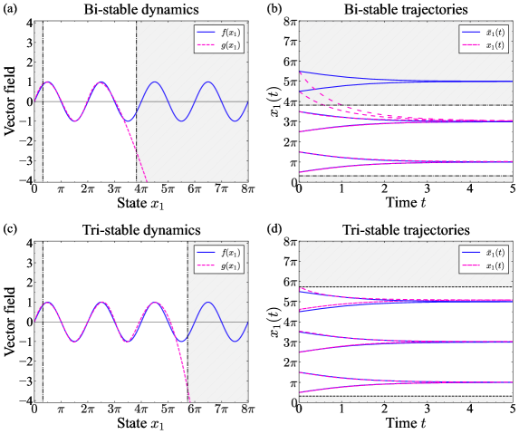
Figure 2: RNCRN approximations of a multi-stable non-polynomial target system. (a) The vector field of the target system (10) and reduced system (11) when $\mathbb{K}_{1}=[1,12]$. (b) Solutions $\bar{x}_{1}(t)$ of the target system (10), and $x_{1}(t)$ of the full system (12) with $\mu=0.01$. Analogous plots are shown in panels (c) and (d) for the tri-stable RNCRN over $\mathbb{K}_{1}=[1,18]$ from Appendix C.1, whose reduced and full ODEs are given respectively by (28) and (29), with coefficients (27) and $\mu=0.01$. In panels (c) and (d), the initial concentrations of all chemical perceptrons are set to zero.

Dynamical approximation. Let us apply the second step from Algorithm 1. Using the coefficients from (11), we now form the full ODEs (see (8)):

$$\frac{\mathrm{d}x_{1}}{\mathrm{d}t} =-0.983x_{1}y_{1}-0.050x_{1}y_{2}+2.398x_{1}y_{3}, x_{1}(0)=a_{1}\in\mathbb{K}_{1},$$

$$\mu\frac{\mathrm{d}y_{1}}{\mathrm{d}t} =1-1.167x_{1}y_{1}+7.789y_{1}-y_{1}^{2}, y_{1}(0)=b_{1}\geq 0,$$

$$\mu\frac{\mathrm{d}y_{2}}{\mathrm{d}t} =1+0.994x_{1}y_{2}-1.918y_{2}-y_{2}^{2}, y_{2}(0)=b_{2}\geq 0,$$

$$\mu\frac{\mathrm{d}y_{3}}{\mathrm{d}t} =1-0.730x_{1}y_{3}+3.574y_{3}-y_{3}^{2}, y_{3}(0)=b_{3}\geq 0.$$ (12)

We fix the initial conditions arbitrarily to $b_{1}=b_{2}=b_{3}=0$, the desired final-time to $T=5$ and the perceptron speed to $\mu=0.01$. We numerically integrate (10) and (12) over $t\in[0,5]$ for a fixed initial concentration $a_{1}\in\mathbb{K}_{1}$ of the executive species, and plot the solutions $\bar{x}(t)$ and $x(t)$; we then repeat the same computations for various values of $a_{1}$, which we display in Figure 2(b). One can notice that the RNCRN underlying (12) with $\mu=0.01$ accurately approximates the time-trajectories of the target system; in particular, we observe bi-stability.

Tri-stability. Let us now apply Algorithm 1 on (10) to obtain a tri-stable RNCRN. To this end, we consider a larger set $\mathbb{K}_{1}=[1,18]$, which includes three stable equilibria, $\pi$, $3\pi$, and $5\pi$, and two unstable equilibria, $2\pi$ and $4\pi$. Applying Algorithm 1, we find an RNCRN with $M=4$ chemical perceptrons, which with $\mu=0.01$ displays the desired tri-stability; see Figure 2(c)–(d), and see Appendix C.1 for more details. In a similar manner, Algorithm 1 can be used to achieve RNCRNs with arbitrary number of stable equilibria.

4.2 Oscillations

Let us consider the two-variable target ODE system

$$\frac{\mathrm{d}\bar{x}_{1}}{\mathrm{d}t} =f_{1}(\bar{x}_{1},\bar{x}_{2})=6+4J_{0}\left(\frac{3}{2}\bar{x}_{1}\right)-\bar{x}_{2}, \bar{x}_{1}(0)=a_{1}\geq 0,$$

$$\frac{d\bar{x}_{2}}{dt} =f_{2}(\bar{x}_{1},\bar{x}_{2})=\bar{x}_{1}-4, \bar{x}_{2}(0)=a_{2}\geq 0,$$ (13)

were $J_{0}(\bar{x}_{1})$ is the Bessel function of the first kind. Numerical simulations suggest that (13) has an isolated oscillatory solution, which we display as the blue curve in the $(\bar{x}_{1},\bar{x}_{2})$-space in Figures 3(a); also shown as grey arrows is the vector field, and as the unshaded box we display the desired region of interest $\mathbb{K}_{1}\times\mathbb{K}_{2}=[0.1,12]\times[0.1,12]$. In Figure 3(c)–(d), we show as solid blue curves this oscillatory solution in the $(t,\bar{x}_{1})$- and $(t,\bar{x}_{2})$-space, respectively.

Using Algorithm 1, we find an RNCRN with $M=6$ chemical perceptrons, whose dynamics with $\mu=0.01$ qualitatively matches the dynamics of the target system (13) within the region of interest; see Appendix C.2 for details. We display the solution of this RNCRN as the purple curve in Figures 3(b)–(d).

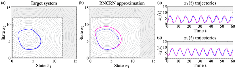
Figure 3: RNCRN approximation of an oscillatory non-polynomial target system. (a) The vector field of the target system (13) (grey arrows) for $\mathbb{K}_{1}\times\mathbb{K}_{2}=[0.1,12]\times[0.1,12]$, and a solution of (13) with $\bar{x}_{1}(0)=2$ and $\bar{x}_{2}(0)=4$ (blue). (b) Analogous plot is shown for the RNCRN from Appendix C.2, whose reduced and full ODEs are given respectively by (31) and (32), with coefficients (30) and $\mu=0.01$. The vector field of (31) (grey arrows) is shown over $\mathbb{K}_{1}\times\mathbb{K}_{2}$, together with a solution of (32) (purple). Panels (c) and (d) respectively display the solutions $\bar{x}_{1}(t)$ and $x_{1}(t)$, and $\bar{x}_{2}(t)$ and $x_{2}(t)$. In all the panels, the same $x_{1}(0)$ and $x_{2}(0)$ are used, and initial concentrations of the chemical perceptrons are all set to zero.

4.3 Chaos

As our final example, we consider the three-variable target ODE system

$$\frac{\mathrm{d}\bar{x}_{1}}{\mathrm{d}t} =f_{1}(\bar{x}_{1},\bar{x}_{2},\bar{x}_{3})=2.5\bar{x}_{1}(1-1.5\bar{x}_{1})-\frac{4\bar{x}_{1}\bar{x}_{2}}{1+3\bar{x}_{1}}, \bar{x}_{1}(0)=0.25,$$

$$\frac{\mathrm{d}\bar{x}_{2}}{\mathrm{d}t} =f_{2}(\bar{x}_{1},\bar{x}_{2},\bar{x}_{3})=-0.4\bar{x}_{2}+\frac{4\bar{x}_{1}\bar{x}_{2}}{1+3\bar{x}_{1}}-\frac{4\bar{x}_{2}\bar{x}_{3}}{1+3\bar{x}_{2}}, \bar{x}_{2}(0)=0.25,$$

$$\frac{\mathrm{d}\bar{x}_{3}}{\mathrm{d}t} =f_{3}(\bar{x}_{1},\bar{x}_{2},\bar{x}_{3})=-0.6\bar{x}_{3}+\frac{4\bar{x}_{2}\bar{x}_{3}}{1+3\bar{x}_{2}}, \bar{x}_{3}(0)=0.25.$$ (14)

ODEs (14) are known as the Hasting-Powell system [45], and have been reported to exhibit chaotic behaviour. We present a portion of the state-space of (14) in Figure 4(a).

Using Algorithm 1, we find an RNCRN with $M=5$ chemical perceptrons to approximate the dynamics of the Hasting-Powell system (14) over the compact set $x_{1}\in\mathbb{K}_{1}$, $x_{2}\in\mathbb{K}_{2}$ and $x_{2}\in\mathbb{K}_{3}$ with $\mathbb{K}_{1}=\mathbb{K}_{2}=\mathbb{K}_{3}=[0.01,1]$. The parameters and the RREs can be found in Appendix C.3. The state-space for the executive species from the RNCRN is presented in Figure 4(b) when $\mu=0.1$, suggesting presence of a chaotic attractor, in qualitative agreement with Figure 4(a). In Figure 4(c)–(e), we display the underlying time-trajectories. Alignment of the trajectories is not expected for long periods of time due to the chaotic nature of the target system (causing exponential divergence of nearby trajectories).

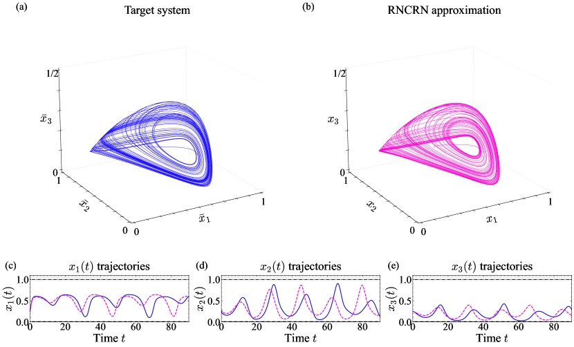
Figure 4: RNCRN approximation of a non-polynomial target system with a chaotic attractor. (a) Solution of target system (14) with $\bar{x}_{1}(0)=\bar{x}_{2}(0)=\bar{x}_{3}(0)=0.25$. (b) Solution of the full ODEs system (35) for the RNCRN from Appendix C.3 with coefficients (33), $\mu=0.1$, and initial conditions $x_{1}(0)=x_{2}(0)=x_{3}(0)=0.25$, and zero initial conditions for all chemical perceptrons. Panels (c), (d) and (e) respectively display the solutions $\bar{x}_{1}(t)$ and $x_{1}(t)$, $\bar{x}_{2}(t)$ and $x_{2}(t)$ and $\bar{x}_{1}(t)$ and $x_{1}(t)$.

5 Discussion

In this paper, we have introduced a class of CRNs that can be trained to approximate the dynamics of any well-behaved system of ordinary-differential equations (ODEs). These recurrent neural chemical reaction networks (RNCRNs) operate by continually actuating the concentration of the executive chemical species such that they adhere to a vector field which has been encoded by a faster system of chemical perceptrons. In Theorem A.1 in Appendix A, we have presented the approximation abilities of RNCRNs. Based on this result, we have put forward Algorithm 1 for training RNCRNs, which relies on the backpropagation algorithm from ANN theory. Due to the nature of the backpropagation procedure, Algorithm 1 is not guaranteed to find an optimal solution; nevertheless, Algorithm 1 proved effective for the target systems presented in this paper. In particular, in Section 4, we showcased examples of RNCRNs that replicate sophisticated dynamical behaviours with up to six chemical perceptrons, which are at most two orders of magnitude faster than the executive species.

RNCRNs contain only chemical reactions of certain kind (e.g. see (1)), all of which are at most bi-molecular, which is suitable for experimental implementations via DNA strand-displacement technologies [46]. In particular, arbitrary bi-molecular CRNs, whose rate coefficients span up to six orders of magnitude [47], can be implemented with DNA strand-displacement reactions, and this approach has achieved chemical systems with more than 100 chemical species [31, 32]. Let us stress that high-precision calibration of the initial concentrations of chemical species within this framework is not feasible [38]. In this context, an advantage of the RNCRNs is that the bulk of the underlying species, namely the chemical perceptrons, have arbitrary initial conditions.

While RNCRNs are experimentally feasible, such chemical-based machine learning suffers from several idiosyncrasies that are not present in traditional electronic-based machine learning. Firstly, adding a perceptron or new weight to an ANN is trivial compared to adding a chemical perceptron to an RNCRN, which requires introducing a specially engineered chemical species. Secondly, chemical systems are prone to unintended reactions, so that the modularity of each chemical perceptron might break down as the network scales in size [25]. Finally, the weight parameters of an ANN can be fine-tuned to a high degree of precision. However, despite techniques to modulate the effective rates of chemical reactions, the calibration of reaction rates is significantly less precise than in electronic circuits [47, 48].

RNCRNs allow one to map ODEs with non-polynomial right-hand sides to dynamically similar reaction-rate equations (RREs). Alternative methods put forward in the literature solve this problem in two steps: firstly, the non-polynomial ODEs are mapped to polynomial ones and, secondly, special maps are then applied to transform these polynomial ODEs to RREs. Although the second step can be performed efficiently [43, 49, 50, 51, 52, 53], the first step suffers from a significant drawback, which is not a feature of the RNCRNs: the initial conditions for the auxiliary species are constrained. For example, applying the standard method from [36, 37] to the target non-polynomial system (10), one obtains polynomial ODEs given by

$$\frac{\mathrm{d}x_{1}}{\mathrm{d}t} =y_{1}, x_{1}(0)=a_{1},$$

$$\frac{\mathrm{d}y_{1}}{\mathrm{d}t} =y_{1}y_{2}, y_{1}(0)=\sin(a_{1}),$$

$$\frac{\mathrm{d}y_{2}}{\mathrm{d}t} =y_{1}y_{3}, y_{2}(0)=\cos(a_{1}),$$

$$\frac{\mathrm{d}y_{3}}{\mathrm{d}t} =y_{2}y_{3}, y_{3}(0)=-\sin(a_{1}).$$ (15)

The solution $x_{1}(t)$ from equation (15) is equivalent to that of $\bar{x}_{1}(t)$ from the target system (10) for all $a_{1}\in\mathbb{R}$. However, the initial conditions for the auxiliary species $y_{1}(0)=\sin(a_{1})$, $y_{2}(0)=\cos(a_{1})$, and $y_{3}(0)=-\sin(a_{1})$ from (15) are constrained. In contrast, the initial concentrations of the auxiliary species from the RNCRN approximation (12) are arbitrary.

As part of the future work, firstly, it is important to study the performance of RNCRNs when the underlying rate coefficients are perturbed; we suspect modifications to the training algorithm might be a strategy to select for robust RNCRNs. Secondly, of importance is also to study how the RNCRNs preform in the low-molecular-count regime, where stochastic effects are significant. Finally, in Appendix B, we have generalized the single-layer (shallow) RNCRNs to multi-layer (deep) ones; in future work, we will study whether such deep RNCRNs have sufficiently advantageous approximation abilities to justify the additional experimental complexity.

6 Declarations

Author Contributions: AD, BQ, TEO, and TP conceptualization the study; AD and TP preformed the mathematical analyses; AD preformed the simulations and wrote the original draft; BQ, TEO, and TP reviewed and edited the final submission.
Funding: Alexander Dack acknowledges funding from the Department of Bioengineering at Imperial College London. Benjamin Qureshi would like to thank the European Research Council (ERC) under the European Union’s Horizon 2020 research and innovation program (Grant agreement No. 851910). Thomas E. Ouldridge would like to thank the Royal Society for a University Research Fellowship. Tomislav Plesa would like to thank Peterhouse, University of Cambridge, for a Fellowship.
Conflict of interest: The authors declare that they have no competing interests.

Appendix A Appendix: Single-layer RNCRN

Consider again the target system (7), and the single-layer RNCRN system (8), whose CRN is given by

$$\varnothing \xrightarrow[]{\beta_{i}}X_{i},\;\;\;\;X_{i}+Y_{j}\xrightarrow[]{\left|\alpha_{i,j}\right|}Y_{j}+X_{i}+\textrm{sign}(\alpha_{i,j})X_{i},$$

$$\varnothing \xrightarrow[]{\gamma/\mu}Y_{j},\;\;\;\;X_{i}+Y_{j}\xrightarrow[]{\left|\omega_{j,i}\right|/\mu}X_{i}+Y_{j}+\textrm{sign}(\omega_{j,i})Y_{j},$$

$$Y_{j} \xrightarrow[]{\left|\omega_{j,0}\right|/\mu}Y_{j}+\textrm{sign}(\omega_{j,0})Y_{j},\;\;\;\;2Y_{j}\xrightarrow[]{1/\mu}Y_{j},$$ (16)

for $i=1,2,\ldots,N$ and $j=1,2,\ldots,M$. We let $\mathbf{x}=(x_{1},x_{2},\ldots,x_{N})\in\mathbb{R}^{N}$, and collect all the rate coefficients $\alpha_{i,j}$ and $\omega_{j,k}$ respectively into suitable vectors $\boldsymbol{\alpha}\in\mathbb{R}^{NM}$ and $\boldsymbol{\omega}\in\mathbb{R}^{M(N+1)}$; similarly, we let $\boldsymbol{\beta}=(\beta_{1},\beta_{2},\ldots,\beta_{N})\in\mathbb{R}_{\geq}^{N}$. Furthermore, we define the reduced vector field by

$$g_{i}(\mathbf{x})=g_{i}(\mathbf{x};\boldsymbol{\alpha},\boldsymbol{\beta},\gamma,\boldsymbol{\omega}) =\beta_{i}+x_{i}\sum_{j=1}^{M}\alpha_{i,j}\sigma_{\gamma}\left(\sum_{k=1}^{N}\omega_{j,k}x_{k}+\omega_{j,0}\right),\;\;\;\textrm{for }i=1,2,\ldots,N,$$ (17)

which appears on the right-hand side of (9).

Theorem A.1.

$($Single-layer RNCRN$)$ Consider the target system $(\ref{eq:target_ODEs})$ on a fixed compact set $\mathbb{K}=\mathbb{K}_{1}\times\mathbb{K}_{2}\times\ldots\times\mathbb{K}_{N}\subset\mathbb{R}_{>}^{N}$ in the state-space, with vector field $f_{1},f_{2},\ldots,f_{N}$ Lipschitz-continuous on $\mathbb{K}$. Consider also the single-layer RNCRN system $(\ref{eq:single_layer_RRE})$ with rate coefficients $\boldsymbol{\beta}=\boldsymbol{\beta}^{*}\in\mathbb{R}_{\geq}^{N}$ and $\gamma=\gamma^{*}>0$ fixed.

1. Quasi-static approximation. Consider the reduced vector field $(\ref{eq:reduced_functions})$. Let $\varepsilon>0$ be any given tolerance. Then, for every sufficiently large $M>0$ there exist $\boldsymbol{\alpha}^{*}\in\mathbb{R}^{NM}$ and $\boldsymbol{\omega}^{*}\in\mathbb{R}^{M(N+1)}$ such that

   $$\underset{\mathbf{x}\in\mathbb{K}}{\max}\left|g_{i}(\mathbf{x};\boldsymbol{\alpha}^{*},\boldsymbol{\beta}^{*},\gamma^{*},\boldsymbol{\omega}^{*})-f_{i}(\mathbf{x})\right|\leq\varepsilon\;\;\textrm{for all }i=1,2,\ldots,N.$$ (18)

2. Dynamical approximation. Assume that the solution of $(\ref{eq:target_ODEs})$ exists for all $t\in[0,T]$ for some $T>0$, and that $\bar{x}_{i}(t)\in\mathbb{K}_{i}$ for all $t\in[0,T]$ for all $i=1,2,\ldots,N$. Then, for every sufficiently small $\varepsilon=\varepsilon^{*}>0$ fixed there exists $\mu_{0}>0$ such that for all $\mu\in(0,\mu_{0})$ system $(\ref{eq:single_layer_RRE})$ has a unique solution $x_{i}(t)\in\mathbb{K}_{i}$ for all $t\in[0,T]$ for all $i=1,2,\ldots,N$, and

   $$\underset{t\in[0,T]}{\max}\left|x_{i}(t;\boldsymbol{\alpha}^{*},\boldsymbol{\beta}^{*},\gamma^{*},\boldsymbol{\omega}^{*},\mu)-\bar{x}_{i}(t)\right| \leq c_{1}\varepsilon^{*}+c_{2}\mu\;\;\textrm{for all }i=1,2,\ldots,N,$$ (19)

   where constants $c_{1}$ and $c_{2}$ are independent of $\mu$.

Proof.

Quasi-static approximation. Consider the continuous function $h_{i}:\mathbb{K}\rightarrow\mathbb{R}$ defined by $h_{i}(\mathbf{x})=(f_{i}(\mathbf{x})-\beta_{i}^{*})/x_{i}$. Since the activation function $\sigma_{\gamma}$, defined by (6), is continuous and non-polynomial, it follows from [54][Theorem 3.1] that for any $\varepsilon>0$ there exist $M>0$, coefficients $\alpha_{i,j}^{*},\omega_{j,k}^{*}\in\mathbb{R}$ and a continuous function $\rho_{i}(\mathbf{x})$ such that

$$h_{i}(\mathbf{x}) =\sum_{j=1}^{M}\alpha_{i,j}^{*}\sigma_{\gamma^{*}}\left(\sum_{k=1}^{N}\omega_{j,k}^{*}x_{k}+\omega_{j,0}^{*}\right)+\rho_{i}(\mathbf{x})\;\;\;\textrm{for all }i=1,2,\ldots,N,$$ (20)

and $\max_{\mathbf{x}\in\mathbb{K}}|\rho_{i}(\mathbf{x})|\leq\varepsilon/X_{i}$, with $X_{i}=\max_{x_{i}\in\mathbb{K}_{i}}x_{i}$. Equation (20) implies (18).

Dynamical approximation. It follows from (18) and regular perturbation theory [55] that there exists $\varepsilon_{0}>0$ such that for all $\varepsilon\in(0,\varepsilon_{0})$

$$\underset{t\in[0,T]}{\max}\left|\tilde{x}_{i}(t;\boldsymbol{\alpha}^{*},\boldsymbol{\beta}^{*},\gamma^{*},\boldsymbol{\omega}^{*})-\bar{x}_{i}(t)\right| \leq c_{1}\varepsilon\;\;\textrm{for all }i=1,2,\ldots,N,$$ (21)

for some $\varepsilon$-independent constant $c_{1}>0$, where $\tilde{x_{i}}(t)=\tilde{x}_{i}(t;\boldsymbol{\alpha}^{*},\boldsymbol{\beta}^{*},\gamma^{*},\boldsymbol{\omega}^{*})$ satisfies the reduced system (9). In what follows, we fix $\varepsilon=\varepsilon^{*}\in(0,\varepsilon_{0})$.

Consider the fast (adjoined) system from (8), defined by

$$\frac{\mathrm{d}y_{j}}{\mathrm{d}\tau} =\gamma^{*}+y_{j}\left(\sum_{i=1}^{N}\omega_{j,i}^{*}x_{i}+\omega_{j,0}^{*}\right)-y_{j}^{2},\hskip 14.22636pty_{j}(0)=b_{j},\;\;\;\textrm{for }j=1,2,\ldots,M,$$ (22)

where $x_{1},x_{2},\ldots,x_{N}$ are parameters. The ODEs from (22) are decoupled, and each one has a unique non-negative continuously differentiable equilibrium $y_{j}=\sigma_{\gamma^{*}}\left(\sum_{k=1}^{N}\omega_{j,k}^{*}x_{k}+\omega_{j,0}^{*}\right)$, which is stable for all non-negative initial conditions $b_{j}\geq 0$. It follows from singular perturbation theory (Tikhonov’s theorem) [56, 57] that there exists $\mu_{0}>0$ such that for all $\mu\in(0,\mu_{0})$ system (8) has a unique solution in $\mathbb{K}$ over time-interval $[0,T]$, and

$$\underset{t\in[0,T]}{\max}\left|x_{i}(t;\boldsymbol{\alpha}^{*},\boldsymbol{\beta}^{*},\gamma^{*},\boldsymbol{\omega}^{*},\mu)-\tilde{x}_{i}(t;\boldsymbol{\alpha}^{*},\boldsymbol{\beta}^{*},\gamma^{*},\boldsymbol{\omega}^{*})\right| \leq c_{2}\mu\;\;\textrm{for all }i=1,2,\ldots,N,$$ (23)

for some $\mu$-independent constant $c_{2}>0$. Using $|x_{i}-\bar{x}_{i}|\leq|x_{i}-\tilde{x}_{i}|+|\tilde{x}_{i}-\bar{x}_{i}|$ and (21) and (23), one obtains (19). ∎

Appendix B Appendix: Multi-layer RNCRN

Multiple layers of perceptrons are common in deep ANNs [4]. Similarly, we construct multi-layer RNCRNs by using the outputs, $Y_{1}^{(1)},\dots,Y_{M_{1}}^{(1)}$ , of a given layer as inputs to the next layer, $Y_{1}^{(2)},\dots,Y_{M_{2}}^{(2)}$. The final layer, $Y_{1}^{(L)},\dots,Y_{M_{L}}^{(L)}$, then feeds back to the executive species $X_{1},\dots,X_{N}$. Stated rigorously as an RRE, we define a $L$-layered RNCRN with $N$ executive species as

$$\frac{\mathrm{d}x_{i}}{\mathrm{d}t} =\beta_{i}+x_{i}\sum_{k=1}^{M_{L}}\alpha_{i,k}y_{k}^{(L)},\;\;x_{i}(0)=a_{i},\;\;\;\textrm{for }i=1,2,\ldots,N,$$

$$\mu\frac{\mathrm{d}y_{j_{1}}^{(1)}}{\mathrm{d}t} =\gamma+\left(\sum_{i=1}^{N}\omega_{j_{1},i}^{(1)}x_{i}+\omega_{j_{1},0}^{(1)}\right)y_{j_{1}}^{(1)}-(y_{j_{1}}^{(1)})^{2},\;\;y_{j_{1}}^{(1)}(0)=b_{j_{1}}\geq 0,\;\;\;\textrm{for }j_{1}=1,2,\ldots,M_{1},$$

$$\vdots$$

$$\mu\frac{\mathrm{d}y_{j_{L}}^{(L)}}{\mathrm{d}t} =\gamma+\left(\sum_{k=1}^{M_{L-1}}\omega_{j_{L},k}^{(L)}y_{k}^{(L-1)}+\omega_{j_{L},0}^{(L)}\right)y_{j_{L}}^{(L)}-(y_{j_{L}}^{(L)})^{2},\;\;y_{j_{L}}^{(1)}(0)=b_{j_{L}}\geq 0,\;\;\;\textrm{for }j_{L}=1,2,\ldots,M_{L}.$$ (24)

The index $i=1,\ldots,N$ enumerates over the executive species whose molecular concentrations are $x_{i}=x_{i}(t)\geq 0$. The index $l=1,\ldots,L$ enumerates over the number of layers in the $L$-layered RNCRN. The compound indices $j_{l}=1,\ldots,M_{l}$ enumerate over the chemical perceptrons within a given layer (each layer may have a different number of chemical perceptrons). The molecular concentration of the chemical perceptrons is $y_{j_{l}}^{(l)}=y_{j_{l}}^{(l)}(t)\geq 0$. There are several parameters $\beta_{i}\geq 0$, $\gamma>0$, $\alpha_{i,j_{l}}\in\mathbb{R}$, and $\omega_{j_{l},j_{l-1}}^{(l)}\in\mathbb{R}$.

Example chemical reaction network. A CRN with the same RRE as equation (24) can be constructed as

$$\varnothing \xrightarrow[]{\beta_{i}}X_{i},\;\;\;\;X_{i}+Y_{j_{L}}^{(L)}\xrightarrow[]{\left|\alpha_{i,j_{L}}\right|}Y_{j_{L}}^{(L)}+X_{i}+\textrm{sign}(\alpha_{i,j_{L}})X_{i},$$

$$\varnothing \xrightarrow[]{\gamma/\mu}Y_{j_{1}}^{(1)},\;\;\;\;X_{i}+Y_{j_{1}}^{(1)}\xrightarrow[]{\left|\omega_{j_{1},i}^{(1)}\right|/\mu}X_{i}+Y_{j_{1}}^{(1)}+\textrm{sign}(\omega_{j_{1},i}^{(1)})Y_{j_{1}}^{(1)},$$

$$Y_{j_{1}}^{(1)} \xrightarrow[]{\left|\omega_{j_{1},0}^{(1)}\right|/\mu}Y_{j_{1}}^{(1)}+\textrm{sign}(\omega_{j_{1},0}^{(1)})Y_{j_{1}}^{(1)},\;\;\;\;2Y_{j_{1}}^{(1)}\xrightarrow[]{1/\mu}Y_{j_{1}}^{(1)},$$

$$\varnothing \xrightarrow[]{\gamma/\mu}Y_{j_{l}}^{(l)},\;\;\;\;Y_{j_{l-1}}^{(l-1)}+Y_{j_{l}}^{(l)}\xrightarrow[]{\left|\omega_{j_{l},j_{l-1}}^{(l)}\right|/\mu}Y_{j_{l-1}}^{(l-1)}+Y_{j_{l}}^{(l)}+\textrm{sign}(\omega_{j_{l},j_{l-1}}^{(l)})Y_{j_{l}}^{(l)},$$

$$Y_{j_{l}}^{(l)} \xrightarrow[]{\left|\omega_{j_{l},0}^{(l)}\right|/\mu}Y_{j_{l}}^{(l)}+\textrm{sign}(\omega_{j_{l},0}^{(l)})Y_{j_{l}}^{(l)},\;\;\;\;2Y_{j_{l}}\xrightarrow[]{1/\mu}Y_{j_{l}},$$ (25)

for $i=1,\ldots,N$ and $l=2,\ldots,L$ such that $j_{l}=1,\ldots,M_{l}$ .

Reduced ODEs. If we formally let $\mu=0$ in (24) we can identify the multi-layered RNCRN’s quasi-static state as

$$\frac{\mathrm{d}x_{i}}{\mathrm{d}t} =g_{i}(x_{1},\ldots,x_{N})=\beta_{i}+x_{i}\sum_{k=1}^{M_{L}}\alpha_{i,k}y_{k}^{(L)},\;\;x_{i}(0)=a_{i}\geq 0,\;\;\;\textrm{for }i=1,2,\ldots,N,$$

$$y_{j_{1}}^{(1)} =\frac{1}{2}\left(\left(\sum_{i=1}^{N}\omega_{j_{1},i}^{(1)}x_{i}+\omega_{j_{1},0}^{(1)}\right)+\sqrt{\left(\sum_{i=1}^{N}\omega_{j_{1},i}^{(1)}x_{i}+\omega_{j_{1},0}^{(1)}\right)^{2}+4\gamma}\right),\;\;y_{j_{1}}^{(1)}(0)=b_{j_{1}}\geq 0,$$

$$\vdots$$

$$y_{j_{L}}^{(L)} =\frac{1}{2}\left(\left(\sum_{k=1}^{M_{L-1}}\omega_{j_{L},k}^{(L)}y_{k}^{(L-1)}+\omega_{j_{L},0}^{(L)}\right)+\sqrt{\left(\sum_{k=1}^{M_{L-1}}\omega_{j_{L},k}^{(L)}y_{k}^{(L-1)}+\omega_{j_{L},0}^{(L)}\right)^{2}+4\gamma}\right),\;\;y_{j_{L}}^{(L)}(0)=b_{j_{L}}\geq 0$$

for $j_{l}=1,2,\ldots,M_{l}$. This is the attractive equilibrium that is reached infinitely fast by the chemical perceptrons if $\mu=0$. Equation (LABEL:eq:multi_layer_RRE_reduced) follows from (24) by applying singular perturbation theory (Tikhonov’s theorem) [56, 57] and stability analysis from [14][Definition 4.7 and Proposition 4.9]. Given equation (LABEL:eq:multi_layer_RRE_reduced) and  [54][Theorem 3.1] it follows that the approximation properties of multi-layer RNCRNs can be formulated similarly to single-layer RNCRNs.

Appendix C Appendix: Examples

C.1 Tri-stable target system

We use Algorithm 1 to approximate the target system (10) on $\mathbb{K}_{1}=[1,18]$. Tolerance $\varepsilon\approx 0.5\times 10^{-3}$ is met with an RNCRN with $M=4$ chemical perceptrons and coefficients $\beta_{1}=0$, $\gamma=1$, and

$$\boldsymbol{\alpha}_{1}=\begin{pmatrix}-4.247\\ 0.487\\ 1.363\\ 0.185\end{pmatrix},\;\;\boldsymbol{\omega}_{0}=\begin{pmatrix}-4.968\\ -3.590\\ -11.236\\ 10.249\end{pmatrix},\;\;\boldsymbol{\omega}_{1}=\begin{pmatrix}0.511\\ 1.043\\ 1.078\\ -2.355\end{pmatrix},$$ (27)

where $\boldsymbol{\alpha}_{1}=(\alpha_{1,1},\alpha_{1,2},\alpha_{1,3},\alpha_{1,4})^{\top}$ and $\boldsymbol{\omega_{k}}=(\omega_{1,k},\omega_{2,k},\omega_{3,k},\omega_{4,k})^{\top}$ for $k=0,1$. The reduced ODE is given by

$$\frac{\mathrm{d}\tilde{x}_{1}}{\mathrm{d}t} =g_{1}(\tilde{x}_{1})=\tilde{x}_{1}\sum_{j=1}^{4}\alpha_{1,j}\sigma_{1}\left(\omega_{j,1}\tilde{x}_{1}+\omega_{j,0}\right),$$ (28)

while the full ODEs read

$$\frac{\mathrm{d}x_{1}}{\mathrm{d}t} =x_{1}\left(\sum_{j=1}^{4}\alpha_{1,j}y_{j}\right), x_{1}(0)=a_{1}\in\mathbb{K}_{1},$$

$$\mu\frac{\mathrm{d}y_{1}}{\mathrm{d}t} =1+\left(\omega_{1,1}x_{1}+\omega_{1,0}\right)y_{1}-y_{1}^{2}, y_{1}(0)=b_{1}\geq 0,$$

$$\mu\frac{\mathrm{d}y_{2}}{\mathrm{d}t} =1+\left(\omega_{2,1}x_{1}+\omega_{2,0}\right)y_{2}-y_{2}^{2}, y_{2}(0)=b_{2}\geq 0,$$

$$\mu\frac{\mathrm{d}y_{3}}{\mathrm{d}t} =1+\left(\omega_{3,1}x_{1}+\omega_{3,0}\right)y_{3}-y_{3}^{2}, y_{3}(0)=b_{3}\geq 0,$$

$$\mu\frac{\mathrm{d}y_{4}}{\mathrm{d}t} =1+\left(\omega_{4,1}x_{1}+\omega_{4,0}\right)y_{4}-y_{4}^{2}, y_{4}(0)=b_{4}\geq 0.$$ (29)

C.2 Oscillatory target system

We use Algorithm 1 to approximate the target system (13) on $\mathbb{K}_{1}\times\mathbb{K}_{2}=[0.1,12]\times[0.1,12]$. Tolerance $\varepsilon\approx 10^{1}$ is met with an RNCRN with $M=6$ chemical perceptrons and coefficients $\beta_{1}=\beta_{2}=1$, $\gamma=1$, and

$$\boldsymbol{\alpha}_{1} =\begin{pmatrix}-1.413\\ -0.189\\ -0.261\\ -0.523\\ 5.437\\ 1.820\\ \end{pmatrix},\;\;\boldsymbol{\alpha}_{2}=\begin{pmatrix}-0.074\\ 8.391\\ -8.387\\ -0.053\\ 0.226\\ 0.307\end{pmatrix},\;\;\boldsymbol{\omega}_{0} =\begin{pmatrix}5.908\\ -1.904\\ 0.753\\ -6.183\\ 3.721\\ -2.744\end{pmatrix},\;\;\boldsymbol{\omega_{1}}=\begin{pmatrix}-1.744\\ 0.244\\ -0.299\\ 1.411\\ -1.820\\ 0.495\end{pmatrix},\;\;\boldsymbol{\omega_{2}}=\begin{pmatrix}0.061\\ -1.009\\ -0.879\\ 0.716\\ -0.221\\ 0.152\end{pmatrix},$$ (30)

where $\boldsymbol{\alpha}_{i}=(\alpha_{i,1},\alpha_{i,2},\ldots,\alpha_{i,6})^{\top}$ for $i=1,2$, and $\boldsymbol{\omega_{k}}=(\omega_{1,k},\omega_{2,k},\ldots,\omega_{6,k})^{\top}$ for $k=0,1,2$. The reduced ODEs are given by

$$\frac{\mathrm{d}\tilde{x}_{1}}{\mathrm{d}t} =g_{1}(\tilde{x}_{1},\tilde{x}_{2})=1+\tilde{x}_{1}\sum_{j=1}^{6}\alpha_{1,j}\sigma_{1}\left(\omega_{j,1}\tilde{x}_{1}+\omega_{j,2}\tilde{x}_{2}+\omega_{j,0}\right),$$

$$\frac{\mathrm{d}\tilde{x}_{2}}{\mathrm{d}t} =g_{2}(\tilde{x}_{1},\tilde{x}_{2})=1+\tilde{x}_{2}\sum_{j=1}^{6}\alpha_{2,j}\sigma_{1}\left(\omega_{j,1}\tilde{x}_{1}+\omega_{j,2}\tilde{x}_{2}+\omega_{j,0}\right),$$ (31)

while the full ODEs read

$$\frac{\mathrm{d}x_{1}}{\mathrm{d}t} =1+x_{1}\left(\sum_{j=1}^{6}\alpha_{1,j}y_{j}\right),\;\;\frac{\mathrm{d}x_{2}}{\mathrm{d}t}=1+x_{2}\left(\sum_{j=1}^{6}\alpha_{2,j}y_{j}\right),$$

$$\mu\frac{\mathrm{d}y_{1}}{\mathrm{d}t} =1+\left(\sum_{i=1}^{2}\omega_{1,i}x_{i}+\omega_{1,0}\right)y_{1}-y_{1}^{2},\;\;\mu\frac{\mathrm{d}y_{2}}{\mathrm{d}t}=1+\left(\sum_{i=1}^{2}\omega_{2,i}x_{i}+\omega_{2,0}\right)y_{2}-y_{2}^{2},$$

$$\mu\frac{\mathrm{d}y_{3}}{\mathrm{d}t} =1+\left(\sum_{i=1}^{2}\omega_{3,i}x_{i}+\omega_{3,0}\right)y_{3}-y_{3}^{2},\;\;\mu\frac{\mathrm{d}y_{4}}{\mathrm{d}t}=1+\left(\sum_{i=1}^{2}\omega_{4,i}x_{i}+\omega_{4,0}\right)y_{4}-y_{4}^{2},$$

$$\mu\frac{\mathrm{d}y_{5}}{\mathrm{d}t} =1+\left(\sum_{i=1}^{2}\omega_{5,i}x_{i}+\omega_{5,0}\right)y_{5}-y_{5}^{2},\;\;\mu\frac{\mathrm{d}y_{6}}{\mathrm{d}t}=1+\left(\sum_{i=1}^{2}\omega_{6,i}x_{i}+\omega_{6,0}\right)y_{6}-y_{6}^{2}.$$ (32)

Here, we assume general initial concentrations: $x_{1}(0)=a_{1}\in\mathbb{K}_{1}$, $x_{2}(0)=a_{2}\in\mathbb{K}_{2}$, and $y_{1}(0)=b_{1}\geq 0$, $y_{2}(0)=b_{2}\geq 0$, $y_{3}(0)=b_{3}\geq 0$, $y_{4}(0)=b_{4}\geq 0$, $y_{5}(0)=b_{5}\geq 0$, and $y_{6}(0)=b_{6}\geq 0$. The coefficients were rounded to 3 decimal places before being used in simulations.

C.3 Chaotic target system

We use Algorithm 1 to approximate the target system (14) on $x_{1}\in\mathbb{K}_{1}$, $x_{2}\in\mathbb{K}_{2}$ and $x_{2}\in\mathbb{K}_{3}$ with $\mathbb{K}_{1}=\mathbb{K}_{2}=\mathbb{K}_{3}=[0.01,1]$. Tolerance $\varepsilon\approx 10^{2}$ is met with an RNCRN with $M=5$ chemical perceptrons and coefficients $\beta_{1}=\beta_{2}=\beta_{3}=0$, $\gamma=1$, and

$$\boldsymbol{\alpha}_{1} =\begin{pmatrix}-0.272\\ 2.996\\ 0.862\\ -0.244\\ 1.276\\ \end{pmatrix},\;\;\boldsymbol{\alpha}_{2}=\begin{pmatrix}0.109\\ 24.039\\ -5.668\\ -0.057\\ -9.584\\ \end{pmatrix},\;\;\boldsymbol{\alpha}_{3}=\begin{pmatrix}0.026\\ -0.529\\ -1.101\\ 0.034\\ 1.065\end{pmatrix},\;\;$$

$$\boldsymbol{\omega}_{0} =\begin{pmatrix}0.284\\ -1.589\\ -0.178\\ 1.212\\ -0.707\end{pmatrix},\;\;\boldsymbol{\omega}_{1}=\begin{pmatrix}-5.049\\ 0.148\\ 0.506\\ 15.973\\ -1.151\\ \end{pmatrix},\;\;\boldsymbol{\omega}_{2}=\begin{pmatrix}8.895\\ -2.951\\ -4.504\\ -7.781\\ -0.606\\ \end{pmatrix},\;\;\boldsymbol{\omega}_{3}=\begin{pmatrix}-0.068\\ -0.525\\ 0.329\\ -0.027\\ 0.199\\ \end{pmatrix},$$ (33)

where $\boldsymbol{\alpha}_{i}=(\alpha_{i,1},\alpha_{i,2},\ldots,\alpha_{i,5})^{\top}$ for $i=1,2,3$, and $\boldsymbol{\omega_{k}}=(\omega_{1,k},\omega_{2,k},\ldots,\omega_{5,k})^{\top}$ for $k=0,1,2,3$. The reduced ODEs are given by

$$\frac{\mathrm{d}\tilde{x}_{1}}{\mathrm{d}t} =g_{1}(\tilde{x}_{1},\tilde{x}_{2},\tilde{x}_{3})=\tilde{x}_{1}\sum_{j=1}^{5}\alpha_{1,j}\sigma_{1}\left(\omega_{j,1}\tilde{x}_{1}+\omega_{j,2}\tilde{x}_{2}+\omega_{j,3}\tilde{x}_{3}+\omega_{j,0}\right),$$

$$\frac{\mathrm{d}\tilde{x}_{2}}{\mathrm{d}t} =g_{2}(\tilde{x}_{1},\tilde{x}_{2},\tilde{x}_{3})=\tilde{x}_{2}\sum_{j=1}^{5}\alpha_{2,j}\sigma_{1}\left(\omega_{j,1}\tilde{x}_{1}+\omega_{j,2}\tilde{x}_{2}+\omega_{j,3}\tilde{x}_{3}+\omega_{j,0}\right),$$

$$\frac{\mathrm{d}\tilde{x}_{3}}{\mathrm{d}t} =g_{3}(\tilde{x}_{1},\tilde{x}_{2},\tilde{x}_{3})=\tilde{x}_{3}\sum_{j=1}^{5}\alpha_{3,j}\sigma_{1}\left(\omega_{j,1}\tilde{x}_{1}+\omega_{j,2}\tilde{x}_{2}+\omega_{j,3}\tilde{x}_{3}+\omega_{j,0}\right),$$ (34)

while the full ODEs read

$$\frac{\mathrm{d}x_{1}}{\mathrm{d}t} =x_{1}\left(\sum_{j=1}^{5}\alpha_{1,j}y_{j}\right),\;\;\frac{\mathrm{d}x_{2}}{\mathrm{d}t}=x_{2}\left(\sum_{j=1}^{5}\alpha_{2,j}y_{j}\right),\;\;\frac{\mathrm{d}x_{3}}{\mathrm{d}t}=x_{3}\left(\sum_{j=1}^{5}\alpha_{3,j}y_{j}\right),$$

$$\mu\frac{\mathrm{d}y_{1}}{\mathrm{d}t} =1+\left(\sum_{i=1}^{3}\omega_{1,i}x_{i}+\omega_{1,0}\right)y_{1}-y_{1}^{2},\;\;\mu\frac{\mathrm{d}y_{2}}{\mathrm{d}t}=1+\left(\sum_{i=1}^{3}\omega_{2,i}x_{i}+\omega_{2,0}\right)y_{2}-y_{2}^{2},$$

$$\mu\frac{\mathrm{d}y_{3}}{\mathrm{d}t} =1+\left(\sum_{i=1}^{3}\omega_{3,i}x_{i}+\omega_{3,0}\right)y_{3}-y_{3}^{2},\;\;\mu\frac{\mathrm{d}y_{4}}{\mathrm{d}t}=1+\left(\sum_{i=1}^{3}\omega_{4,i}x_{i}+\omega_{4,0}\right)y_{4}-y_{4}^{2},$$

$$\mu\frac{\mathrm{d}y_{5}}{\mathrm{d}t} =1+\left(\sum_{i=1}^{3}\omega_{5,i}x_{i}+\omega_{5,0}\right)y_{5}-y_{5}^{2}.$$ (35)

Here, we assume general initial concentrations: $x_{1}(0)=a_{1}\in\mathbb{K}_{1}$, $x_{2}(0)=a_{2}\in\mathbb{K}_{2}$, $x_{3}(0)=a_{3}\in\mathbb{K}_{3}$ and $y_{1}(0)=b_{1}\geq 0$, $y_{2}(0)=b_{2}\geq 0$, $y_{3}(0)=b_{3}\geq 0$, $y_{4}(0)=b_{4}\geq 0$, and $y_{5}(0)=b_{5}\geq 0$. The coefficients were rounded to 3 decimal places before being used in simulations.

References

- [1] W. S. McCulloch and W. Pitts, “A logical calculus of ideas immanent in nervous activity,” Bulletin of Mathematical Biophysics, vol. 5, pp. 115–133, 1943.
- [2] G. Cybenko, “Approximation by superpositions of a sigmoidal function,” Mathematics of Control, Signals, and Systems, vol. 2, pp. 303–314, 1989.
- [3] K. Hornik, M. Stinchcombe, and H. White, “Multilayer feedforward networks are universal approximators,” Neural Networks, vol. 2, pp. 359–366, 1989.
- [4] Y. LeCun, Y. Bengio, and G. Hinton, “Deep learning,” Nature, vol. 521, pp. 436–444, 2015.
- [5] M. A. Bucci, O. Semeraro, A. Allauzen, G. Wisniewski, L. Cordier, and L. Mathelin, “Control of chaotic systems by deep reinforcement learning,” Proceedings of the Royal Society A: Mathematical, Physical and Engineering Sciences, vol. 475, p. 20190351, 2019.
- [6] A. Hjelmfelt, E. D. Weinberger, and J. Ross, “Chemical implementation of neural networks and Turing machines.,” Proceedings of the National Academy of Sciences, vol. 88, pp. 10983–10987, 1991.
- [7] L. Qian, E. Winfree, and J. Bruck, “Neural network computation with DNA strand displacement cascades,” Nature, vol. 475, pp. 368–372, 2011.
- [8] J. Kim, J. Hopfield, and E. Winfree, “Neural Network Computation by In Vitro Transcriptional Circuits,” Advances in Neural Information Processing Systems, vol. 17, 2004.
- [9] H.-J. K. Chiang, J.-H. R. Jiang, and F. Fages, “Reconfigurable neuromorphic computation in biochemical systems,” in 2015 37th Annual International Conference of the IEEE Engineering in Medicine and Biology Society (EMBC), pp. 937–940, 2015.
- [10] W. Poole, A. Ortiz-Muñoz, A. Behera, N. S. Jones, T. E. Ouldridge, E. Winfree, and M. Gopalkrishnan, “Chemical Boltzmann Machines,” in DNA 2017: DNA Computing and Molecular Programming, vol. 10467, pp. 210–231, 2017.
- [11] A. Moorman, C. C. Samaniego, C. Maley, and R. Weiss, “A Dynamical Biomolecular Neural Network,” in 2019 IEEE 58th Conference on Decision and Control (CDC), pp. 1797–1802, 2019. ISSN: 2576-2370.
- [12] M. Vasić, C. Chalk, A. Luchsinger, S. Khurshid, and D. Soloveichik, “Programming and training rate-independent chemical reaction networks,” Proceedings of the National Academy of Sciences, vol. 119, p. e2111552119, 2022.
- [13] J. Linder, Y.-J. Chen, D. Wong, G. Seelig, L. Ceze, and K. Strauss, “Robust Digital Molecular Design of Binarized Neural Networks,” in 27th International Conference on DNA Computing and Molecular Programming (DNA 27), vol. 205, pp. 1:1–1:20, 2021.
- [14] D. F. Anderson, B. Joshi, and A. Deshpande, “On reaction network implementations of neural networks,” Journal of The Royal Society Interface, vol. 18, p. 20210031, 2021.
- [15] J. Fil, N. Dalchau, and D. Chu, “Programming Molecular Systems To Emulate a Learning Spiking Neuron,” ACS Synthetic Biology, vol. 11, pp. 1992–2220, 2022.
- [16] A. J. Genot, T. Fujii, and Y. Rondelez, “Scaling down DNA circuits with competitive neural networks,” Journal of The Royal Society Interface, vol. 10, p. 20130212, 2013.
- [17] R. Lopez, R. Wang, and G. Seelig, “A molecular multi-gene classifier for disease diagnostics,” Nature Chemistry, vol. 10, pp. 746–754, 2018.
- [18] A. Pandi, M. Koch, P. L. Voyvodic, P. Soudier, J. Bonnet, M. Kushwaha, and J.-L. Faulon, “Metabolic perceptrons for neural computing in biological systems,” Nature Communications, vol. 10, p. 3880, 2019.
- [19] X. Li, L. Rizik, V. Kravchik, M. Khoury, N. Korin, and R. Daniel, “Synthetic neural-like computing in microbial consortia for pattern recognition,” Nature Communications, vol. 12, p. 3139, 2021.
- [20] S. Okumura, G. Gines, N. Lobato-Dauzier, A. Baccouche, R. Deteix, T. Fujii, Y. Rondelez, and A. J. Genot, “Nonlinear decision-making with enzymatic neural networks,” Nature, vol. 610, pp. 496–501, 2022.
- [21] A. J. Van Der Linden, P. A. Pieters, M. W. Bartelds, B. L. Nathalia, P. Yin, W. T. S. Huck, J. Kim, and T. F. A. De Greef, “DNA Input Classification by a Riboregulator-Based Cell-Free Perceptron,” ACS Synthetic Biology, vol. 11, pp. 1510–1520, 2022.
- [22] L. Cardelli, M. Tribastone, and M. Tschaikowski, “From electric circuits to chemical networks,” Natural Computing, vol. 19, pp. 237–248, 2020.
- [23] A. Arkin and J. Ross, “Computational functions in biochemical reaction networks,” Biophysical Journal, vol. 67, pp. 560–578, 1994.
- [24] G. Seelig, D. Soloveichik, D. Y. Zhang, and E. Winfree, “Enzyme-Free Nucleic Acid Logic Circuits,” Science, vol. 314, pp. 1585–1588, 2006.
- [25] L. Qian and E. Winfree, “Scaling Up Digital Circuit Computation with DNA Strand Displacement Cascades,” Science, vol. 332, pp. 1196–1201, 2011.
- [26] D. Del Vecchio, A. J. Dy, and Y. Qian, “Control theory meets synthetic biology,” Journal of The Royal Society Interface, vol. 13, p. 20160380, 2016.
- [27] C. Briat, A. Gupta, and M. Khammash, “Antithetic Integral Feedback Ensures Robust Perfect Adaptation in Noisy Biomolecular Networks,” Cell Systems, vol. 2, pp. 15–26, 2016.
- [28] T. Plesa, G.-B. Stan, T. E. Ouldridge, and W. Bae, “Quasi-robust control of biochemical reaction networks via stochastic morphing,” Journal of The Royal Society Interface, vol. 18, p. 20200985, 2021.
- [29] C. Kieffer, A. J. Genot, Y. Rondelez, and G. Gines, “Molecular Computation for Molecular Classification,” Advanced Biology, vol. 7, p. 2200203, 2023.
- [30] C. C. Samaniego, E. Wallace, F. Blanchini, E. Franco, and G. Giordano, “Neural networks built from enzymatic reactions can operate as linear and nonlinear classifiers,” bioRxiv, 2024.
- [31] K. M. Cherry and L. Qian, “Scaling up molecular pattern recognition with DNA-based winner-take-all neural networks,” Nature, vol. 559, pp. 370–376, 2018.
- [32] X. Xiong, T. Zhu, Y. Zhu, M. Cao, J. Xiao, L. Li, F. Wang, C. Fan, and H. Pei, “Molecular convolutional neural networks with DNA regulatory circuits,” Nature Machine Intelligence, vol. 4, pp. 625–635, 2022.
- [33] W. Xiong and J. E. Ferrell, “A positive-feedback-based bistable ‘memory module’ that governs a cell fate decision,” Nature, vol. 426, pp. 460–465, Nov. 2003.
- [34] P. E. Hardin, J. C. Hall, and M. Rosbash, “Feedback of the Drosophila period gene product on circadian cycling of its messenger RNA levels,” Nature, vol. 343, pp. 536–540, Feb. 1990.
- [35] M. L. Heltberg, S. Krishna, and M. H. Jensen, “On chaotic dynamics in transcription factors and the associated effects in differential gene regulation,” Nature Communications, vol. 10, p. 71, Jan. 2019.
- [36] E. H. Kerner, “Universal formats for nonlinear ordinary differential systems,” Journal of Mathematical Physics, vol. 22, pp. 1366–1371, 1981.
- [37] K. Kowalski, “Universal formats for nonlinear dynamical systems,” Chemical Physics Letters, vol. 209, pp. 167–170, 1993.
- [38] N. Srinivas, J. Parkin, G. Seelig, E. Winfree, and D. Soloveichik, “Enzyme-free nucleic acid dynamical systems,” Science, vol. 358, p. eaal2052, Dec. 2017.
- [39] M. Feinberg, “Lecture notes on chemical reaction networks,” Lecture Notes, Mathematics Research Center, University of Wisconsin-Madison, 1979.
- [40] T. Wilhelm, “Chemical systems consisting only of elementary steps – a paradigma for nonlinear behavior,” Journal of Mathematical Chemistry, vol. 27, pp. 71–88, 2000.
- [41] T. Plesa, “Stochastic approximations of higher-molecular by bi-molecular reactions,” Journal of Mathematical Biology, vol. 86, p. 28, 2023.
- [42] F. Rosenblatt, The perceptron, a perceiving and recognizing automaton Project Para. Cornell Aeronautical Laboratory, 1957.
- [43] T. Plesa, T. Vejchodský, and R. Erban, “Chemical reaction systems with a homoclinic bifurcation: an inverse problem,” Journal of Mathematical Chemistry, vol. 54, pp. 1884–1915, 2016.
- [44] D. E. Rumelhart, G. E. Hinton, and R. J. Williams, “Learning representations by back-propagating errors,” Nature, vol. 323, pp. 533–536, Oct. 1986.
- [45] L. Stone and D. He, “Chaotic oscillations and cycles in multi-trophic ecological systems,” Journal of Theoretical Biology, vol. 248, pp. 382–390, 2007.
- [46] D. Soloveichik, G. Seelig, and E. Winfree, “DNA as a universal substrate for chemical kinetics,” Proceedings of the National Academy of Sciences, vol. 107, pp. 5393–5398, 2010.
- [47] D. Y. Zhang and E. Winfree, “Control of dna strand displacement kinetics using toehold exchange,” Journal of the American Chemical Society, vol. 131, no. 47, pp. 17303–17314, 2009. PMID: 19894722.
- [48] N. E. C. Haley, T. E. Ouldridge, I. Mullor Ruiz, A. Geraldini, A. A. Louis, J. Bath, and A. J. Turberfield, “Design of hidden thermodynamic driving for non-equilibrium systems via mismatch elimination during DNA strand displacement,” Nature Communications, vol. 11, p. 2562, May 2020.
- [49] N. Samardzija, L. D. Greller, and E. Wasserman, “Nonlinear chemical kinetic schemes derived from mechanical and electrical dynamical systems,” The Journal of Chemical Physics, vol. 90, pp. 2296–2304, 1989.
- [50] D. Poland, “Cooperative catalysis and chemical chaos: a chemical model for the Lorenz equations,” Physica D: Nonlinear Phenomena, vol. 65, pp. 86–99, 1993.
- [51] T. Plesa, T. Vejchodský, and R. Erban, “Test Models for Statistical Inference: Two-Dimensional Reaction Systems Displaying Limit Cycle Bifurcations and Bistability,” in Stochastic Processes, Multiscale Modeling, and Numerical Methods for Computational Cellular Biology, pp. 3–27, 2017.
- [52] T. Plesa, A. Dack, and T. E. Ouldridge, “Integral feedback in synthetic biology: Negative-equilibrium catastrophe (Appendix D),” Journal of Mathematical Chemistry, vol. 61, pp. 1980–2018, 2023.
- [53] K. M. Hangos and G. Szederkényi, “Mass action realizations of reaction kinetic system models on various time scales,” Journal of Physics: Conference Series, vol. 268, p. 012009, 2011.
- [54] A. Pinkus, “Approximation theory of the MLP model in neural networks,” Acta Numerica, vol. 8, pp. 143–195, 1999.
- [55] E. A. Coddington and N. Levinson, Theory of Ordinary Differential Equations. New-York: McGraw-Hill, 1995.
- [56] W. Klonowski, “Simplifying principles for chemical and enzyme reaction kinetics,” Biophysical Chemistry, vol. 18, pp. 73–87, 1983.
- [57] A. N. Tikhonov, “Systems of differential equations containing small parameters in the derivatives,” Mat. Sb. (N.S.), vol. 31(73), pp. 575–586, 1952.