CSI-GPT: Integrating Generative Pre-Trained Transformer with Federated-Tuning to Acquire Downlink Massive MIMO Channels

Abstract

In massive multiple-input multiple-output (MIMO) systems, how to reliably acquire downlink channel state information (CSI) with low overhead is challenging. In this work, by integrating the generative pre-trained Transformer (GPT) with federated-tuning, we propose a CSI-GPT approach to realize efficient downlink CSI acquisition. Specifically, we first propose a Swin Transformer-based channel acquisition network (SWTCAN) to acquire downlink CSI, where pilot signals, downlink channel estimation, and uplink CSI feedback are jointly designed. Furthermore, to solve the problem of insufficient training data, we propose a variational auto-encoder-based channel sample generator (VAE-CSG), which can generate sufficient CSI samples based on a limited number of high-quality CSI data obtained from the current cell. The CSI dataset generated from VAE-CSG will be used for pre-training SWTCAN. To fine-tune the pre-trained SWTCAN for improved performance, we propose an online federated-tuning method, where only a small amount of SWTCAN parameters are unfrozen and updated using over-the-air computation, avoiding the high communication overhead caused by aggregating the complete CSI samples from user equipment (UEs) to the BS for centralized fine-tuning. Simulation results verify the advantages of the proposed SWTCAN and the communication efficiency of the proposed federated-tuning method.

I Introduction

In massive multiple-input multiple-output (MIMO) systems, accurate downlink channel state information (CSI) is crucial for beamforming and resource allocation. However, in frequency division duplexing (FDD) systems, accurate estimation and feedback of downlink CSI with low pilot/feedback overhead is challenging, due to the high-dimensional CSI caused by the large number of antennas at the base station (BS) and the non-reciprocity between uplink and downlink channels [1].

As the channel gains associated with different antennas are correlated, the massive MIMO CSI matrix has the inherent redundancy, which can be exploited to reduce the CSI acquisition overhead [1]. Due to its powerful capabilities of feature perception and extraction, deep learning (DL) has been widely used to process CSI in massive MIMO systems for various tasks [2]. The authors of [3] proposed a DL-based joint pilot design and channel estimation (CE) scheme, where the fully connected (FC) layer and the convolutional neural network (CNN) are used to design the pilot signal and estimate the CSI, respectively. The authors of [4] made improvements to [3] by designing pilot signals on different subcarriers differently to further reduce the pilot overhead. As for CSI feedback, the seminal work [5] proposed an autoencoder (AE)-based end-to-end (E2E) optimization framework, and the authors of [6] improved CSI feedback performance by introducing receptive fields of different sizes for CSI feature extraction.

More recently, as reported in [7, 8], joint design of pilot signals, downlink CE and CSI feedback using DL can further improve the downlink CSI acquisition performance. Another approach to improve the performance is to exploit more advanced neural network (NN) architectures. The authors of [9] investigated the application of Transfomer architecture in various massive MIMO processing tasks, which consistently shows advantages over CNN-based algorithms. With the development of NN architectures, variants of Transformer, e.g., Swin Transformer, have shown better feature capture capability in image processing tasks [10], which is another blessing of DL-based massive MIMO signal processing.

The current DL models [3, 4, 5, 7, 6, 8, 9] need a large amount of high-quality CSI samples for training, which can be obtained from actual measurements or generated from classical channel models, e.g., COST 2100 and clustered delay line (CDL) channel [11]. However, it is either difficult or communication-inefficient to obtain a large number of actual CSI samples in various practical scenarios [12], and it may degrade the NN performance if the features of training dataset and test dataset are not consistent. To overcome this issue, the generative adversarial network (GAN) is employed in [12] to generate CSI training datasets based on only a small amount of CSI measurements. Another promising solution [13] is to use federated learning (FL) to avoid collecting high-dimensional actual CSI samples, thereby reducing the communication overhead considerably. By exploiting gradient compression and over-the-air computation (AirComp), the authors of [14] proposed a communication-efficient FL framework for image classification tasks. To tune a large NN model, e.g., Transformer, in a communication-efficient manner, the authors of [15] utilized FL to fine-tune part of the parameters of a pre-trained Transformer model. The authors of [16, 17, 18] showed the potential of FL-based CE and/or CSI feedback for massive MIMO systems. They also showed that users’ data privacy can be protected by using FL. However, whether FL is more communication-efficient than conventional centralized learning (CL) that requires the feedback of CSI samples from user equipment (UEs) to BS remains unexplored.

In this paper, by integrating the generative pre-trained Transformer (GPT) with federated-tuning, we propose a CSI-GPT approach to realize efficient downlink CSI acquisition. Our main contributions can be summarized as follows.

• We propose a Swin Transformer-based channel acquisition network (SWTCAN) as shown in Fig. 1 to acquire downlink CSI with lower pilot/feedback overhead, where downlink pilot signal, CE and CSI feedback are jointly designed. Our SWTCAN not only retains the extraction capability of the conventional Transformer-based approach [9] but also overcomes its weakness in multi-scale feature extraction. Consequently, lower pilot and feedback overhead can be achieved.

• We propose a variational AE-based channel sample generator (VAE-CSG), which can effectively solve the problem of insufficient high-quality CSI samples. Since channel features in different cells vary dramatically, to maximize the potential of SWTCAN, its training at different BSs should rely on large numbers of CSI samples of the respective cells. However, the number of high-quality CSI samples from the current cell is usually limited. We propose a pre-trained strategy by pre-training VAE-CSG using a large number of CSI samples that typically have different features from those of the current cell. Subsequently, we fine-tune VAE-CSG using a limited number of high-quality CSI samples from the current cell. The fine-tuned VAE-CSG then generates a large number of CSI samples for pre-training SWTCAN.

• Finally, to fine-tune the pre-trained SWTCAN for improved performance, we propose an online federated-tuning method. Only a small amount of SWTCAN parameters (around 11%) are unfrozen and updated using AirComp, avoiding the high communication overhead caused by aggregating the CSI samples from UEs to the BS for centralized fine-tuning.The simulation results demonstrate that in typical cases, the proposed federated-tuning method can reduce uplink communication overhead by up to 34.8% compared to the traditional CL method.

Notation: Boldface lower and upper-case symbols denote column vectors and matrices, respectively. Superscripts $(\cdot)^{\rm T}$ and $(\cdot)^{\rm H}$ denote the transpose and conjugate transpose operators, respectively. $p(\mathbf{x\mid y})$ is the conditional distribution of $\mathbf{x}$ given $\mathbf{y}$. $\mathcal{N}(\mathbf{x};\bm{\mu},\bm{\Sigma})$ means $\mathbf{x}$ following a Gaussian distribution with mean $\bm{\mu}$ and covariance matrix $\bm{\Sigma}$. ${\left\|{\bf{A}}\right\|_{F}}$ and $[{\bf{A}}]_{m,n}$ denote the Frobenius norm and the $m$-th row and $n$-th column element of the matrix ${\bf{A}}$, respectively. $\|{\bf x}\|_{p}$, $[{\bf x}]_{m}$, and $|{\bf x}|_{c}$ denote the ${l_{p}}$ norm, the $m$-th element, and the cardinality of the vector ${\bf x}$, respectively. $\mathbf{I}$ is the identity matrix. $\bf{0}$ is a vector with all the elements being 0.

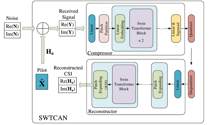
Figure 1: Structure of the proposed SWTCAN.

II Proposed Swin Transformer-Based Downlink CSI Acquisition Scheme

II-A System Model

We assume that the BS deploys a uniform planar array (UPA) with $N_{\rm{BS}}$ antennas to serve $U$ single-antenna UEs in an FDD mode. Orthogonal frequency division multiplexing (OFDM) with $P$ subcarriers is considered. To realize the downlink CSI acquisition, the BS first broadcasts the downlink pilot signal to the UEs, and then each UE estimates the CSI and feeds it back to the BS. We focus on the CE and feedback of a single UE, and its received signal ${\bf{y}}_{p}\!\in\!\mathbb{C}^{M}$ on the $p$-th subcarrier in $M$ successive time slots can be expressed as

$${\bf{y}}_{p}^{\rm T}={\bf{h}}_{p}^{\rm T}{\bf{X}}+{\bf{n}}_{p}^{\rm T},\vspace{-0.5mm}$$ (1)

where ${\bf{X}}\!\in\!\mathbb{C}^{N_{\rm{BS}}\times M}$ is the transmit signal in $M$ successive time slots, ${\bf{h}}_{p}\!\in\!\mathbb{C}^{N_{\rm{BS}}}$ is the $p$-th subcarrier’s channel, and ${\bf{n}}_{p}^{\rm T}$ is complex additive white Gaussian noise (AWGN) with zero mean and covariance matrix $\sigma_{n}^{2}{\bf{I}}$. By stacking the received signals over all the subcarriers, the received signal ${\bf{Y}}\!=\!\left[{\bf{y}}_{1},{\bf{y}}_{2},\cdots,{\bf{y}}_{P}\right]^{\rm T}\!\in\!\mathbb{C}^{P\times M}$ can be written as

$${\bf{Y}}={\bf{H}}_{s}{\bf{X}}+{\bf{N}},\vspace{-0.5mm}$$ (2)

where ${\bf{H}}_{s}=\left[{\bf{h}}_{1},{\bf{h}}_{2},\cdots,{\bf{h}}_{P}\right]^{\rm T}\!\in\!\mathbb{C}^{P\times N_{\rm{BS}}}$ is the frequency-spatial domain channel matrix, and ${\bf{N}}=\left[{\bf{n}}_{1},{\bf{n}}_{2},\cdots,{\bf{n}}_{P}\right]^{\rm T}$ is the AWGN matrix. Furthermore, we can obtain the frequency-angle domain channel ${\bf{H}}_{a}\!\in\!\mathbb{C}^{P\times N_{\rm{BS}}}$ as [1]

$${\bf{H}}_{a}={\bf{H}}_{s}{\bf{F}},\vspace{-0.5mm}$$ (3)

where ${\bf{F}}\!\in\!\mathbb{C}^{N_{\mathrm{BS}}\times N_{\rm{BS}}}$ a discrete Fourier transform (DFT) matrix. Due to the angular-domain sparsity, each row of ${\bf{H}}_{a}$ is a sparse vector. Hence, (2) can be rewritten as

$${\bf{Y}}={\bf{H}}_{a}{\bf{F}}^{\rm H}{\bf{X}}+{\bf{N}}={\bf{H}}_{a}{\widetilde{\bf{X}}}+{\bf{N}},\vspace{-0.5mm}$$ (4)

where ${\widetilde{\bf{X}}}={\bf{F}}^{\rm H}{\bf{X}}$.

II-B Pilot Design and CSI Acquisition

The structure of the proposed SWTCAN is shown in Fig. 1. We use a linear layer without bias to model the pilot design. The received pilot signal is passed through a linear layer, and its dimension is restored to be the same as the channel. The high-dimensional features extracted by Swin Transformer blocks [19] under windows of different sizes are compressed into codewords after the linear layer and sigmoid activation function. The compressed codeword is then quantized into $B$ bits vector $\mathbf{q}$ by a quantization layer. The entire CSI compressor can be expressed as

$$\mathbf{q}=\mathcal{Q}\left(f_{\downarrow}\left(\mathbf{Y},\bm{\theta}_{\downarrow}\right)\right)\in\mathbb{R}^{B},$$ (5)

where $\mathcal{Q}(\cdot)$, $f_{\downarrow}(\cdot,\cdot)$, and $\bm{\theta}_{\downarrow}$ denote the quantization function, compression function and learnable neural network parameters in the compressor, respectively.

The structure of the CSI reconstructor at the BS is similar to that of the compressor. The received bit vector is transformed by a dequantization layer and a linear layer to change the feature dimension, which is then inputted to Swin Transformer blocks. Finally, the features are up-sampled by a patch expanding layer to reconstruct the downlink CSI $\widehat{\mathbf{H}}_{a}$ at the BS. The entire CSI reconstructor can be expressed as

$$\widehat{\mathbf{H}}_{a}=f_{\uparrow}\left(\mathcal{Q}^{-1}\left(\mathbf{q}\right),\bm{\theta}_{\uparrow}\right),$$ (6)

where $f_{\uparrow}(.,.)$, $\mathcal{Q}^{-1}(\cdot)$, and $\bm{\theta}_{\uparrow}$ denote the reconstruction function, dequantization function and learnable neural network parameters, respectively. By adopting the normalized mean squared error (NMSE) $L_{1}\!=\!\frac{\left\|\widehat{\mathbf{H}}_{a}-\mathbf{H}_{a}\right\|_{F}^{2}}{\left\|\mathbf{H}_{a}\right\|_{F}^{2}}$ as the loss function, we can perform E2E training on the proposed SWTCAN.

III Generative Pre-Training and Federated-Tuning for the Proposed SWTCAN

Our proposed CSI-GPT framework integrates the proposed VAE-CSG to pre-train SWTCAN with a small number of CSI samples from the current cell. We also adopt a FL-based online fine-tuning to further improve the performance of pre-trained SWTCAN, which has much lower communication overhead than the CL scheme. The procedure of CSI-GPT with federated-tuning is summarized in Algorithm 1.

III-A Generative AI-Based Pre-Training

The proposed VAE-based generative network for generating CSI samples, called VAE-CSG, pre-trains the SWTCAN so that it can initially learn the generalized CSI features before fine-tuning it, which helps the model to perform better in the subsequent task and accelerate the convergence speed. As shown in line 1 of Algorithm 1, the BS initially pre-trains the VAE-CSG using a large amount of CSI samples generated by the channel simulator, and these samples typically have a different channel distribution from the current cell. Then the VAE-CSG is fine-tuned using a limited number of CSI samples from the current cell, which are obtained from the uplink CE at a high signal-to-noise ratio (SNR).

Algorithm 1 Proposed CSI-GPT with Federated-Tuning

1:  BS pre-trains VAE-CSG with simulated CSI samples, and fine-tunes VAE-CSG with limited CSI samples obtained in current cell to generate more CSI samples.

2:  BS pre-trains SWTCAN with data generated by VAE-CSG.

3:  Initialize federated-tuning parameters $\mathbf{m}_{0}=0$, $\mathbf{v}_{0}=0$.

4:  for $t=1,2,\cdots,T$ do

5:     BS broadcasts $\tilde{\bm{\theta}}_{t}$ to all UEs.

6:     for each UE $u\in\mathcal{S}$ in parallel do

7:        Initialize local parameters $\tilde{\bm{\theta}}^{u,0}_{t}=\tilde{\bm{\theta}}_{t}$.

8:        Use SGD for local model updates, according to (9).

9:     end for

10:     Perform AirComp, according to (10).

11:     BS updates the model parameter $\tilde{\bm{\theta}}_{t+1}$, according to (11).

12:  end for

The VAE-CSG comprises an encoder and a decoder, which are jointly trained using an E2E method and only the decoder is utilized for generating CSI samples. Denote the parameters of the encoder and decoder of VAE-CSG as ${\bm{\psi}}$ and ${\bm{\omega}}$, respectively. The output of the encoder, i.e., the latent variable, is denoted as $\mathbf{z}\!=\!f_{enc}(\mathbf{H}_{a};\bm{\psi})$. Similarly, the output of the decoder is denoted as $f_{dec}(\mathbf{z};\bm{\omega})$. The loss function of the VAE-CSG consists of two parts. The first part is the reconstruction loss, $\|f_{dec}(\mathbf{z};\bm{\omega})\!-\!\mathbf{H}_{a}\|_{F}^{2}$, which measures the closeness of the VAE-CSG’s output to the original input. According to [20], the second part measures the difference between the learned distribution of latent variable $\mathbf{z}$ and the predefined prior distribution $p_{0}(\mathbf{z})\!\sim\!\mathcal{N}(\mathbf{z};\mathbf{0},\mathbf{I})$. Let the learned distribution of $\mathbf{z}$ be $p_{\bm{\psi}}(\mathbf{z}|\mathbf{H}_{a})$. Using Kullback-Leibler (KL) divergence, the second part of the loss is ${\text{D}}_{KL}(p_{\bm{\psi}}(\mathbf{z}|\mathbf{H}_{a})||p_{0}(\mathbf{z}))$. Hence, the loss function of VAE-CSG is expressed as

$$L_{2}(\bm{\psi},\bm{\omega})= \|f_{dec}(\mathbf{z},\bm{\omega})-\mathbf{H}_{a}\|_{F}^{2}$$

$$+l\cdot{\text{D}}_{KL}(p_{\bm{\psi}}(\mathbf{z}|\mathbf{H}_{a})||p_{0}(\mathbf{z})),$$ (7)

where l is a predefined hyper-parameter. The second term in (III-A) enhances the diversity and quality of the generated CSI samples by enforcing the encoder to produce a latent variable that closely matches the standard Gaussian distribution. We use the data generated by VAE-CSG to pre-train SWTCAN (line 2 in Algorithm 1). The performance of pre-trained SWTCAN is suboptimal, since the CSI distributions used in pre-training and testing in practical deployment are usually different.

III-B Federated Learning-Based Online Fine-Tuning

To enhance the performance of the pre-trained SWTCAN, fine-tuning is necessary. Adopting the CL strategy for fine-tuning would require the BS to aggregate a large number of CSI samples from UEs in the current cell, resulting in excessive uplink communication overhead. The downlink CSI used for fine-tuning can be obtained by the BS broadcasting the pilot signals, facilitating each UE to estimate its own downlink CSI based on the pilot signals. To address the high communication overhead and privacy issue caused by feeding these CSI samples back to the BS, we utilize the communication-efficient federated-tuning and AirComp to fine-tune the SWTCAN, while reducing uplink communication costs and overhead.

III-B1 Communication-Efficient Federated-Tuning

Uploading the entire parameter set $\bm{\theta}$ of SWTCAN for fine-tuning would result in prohibitive uplink communication overhead. We opt to freeze the majority parameters of SWTCAN and upload only a minority of the entire parameters, denoted by $\tilde{\bm{\theta}}$. Hence, in federated-tuning, we solve the optimization:

$$\min\nolimits_{\tilde{\bm{\theta}}\in\mathbb{R}^{d}}L_{1}(\tilde{\bm{\theta}})=\frac{1}{U}\sum\nolimits_{u=1}\nolimits^{U}L_{1}^{u}(\tilde{\bm{\theta}}),$$ (8)

where $d\!=\!|\tilde{\bm{\theta}}|_{c}$ is the dimension of the learnable parameters and $L_{1}^{u}(\tilde{\bm{\theta}})$ is the NMSE loss function of the $u$-th UE.

III-B2 AirComp for Efficient Federated-Tuning

To accelerate federated-tuning convergence and minimize the uplink communication rounds, we employ the federated AMSGrad with max stabilization (FedAMS) [21] in conjunction with AirComp. In the $t$-th communication round, $1\leq t\leq T$, the BS broadcasts the learnable model parameter $\tilde{\bm{\theta}}_{t}$ to all UEs (line 5 in Algorithm 1). Due to the heterogeneous user availability, only a fraction of UEs, denoted as $\mathcal{S}$, participates in the $t$-th communication round. The $u$-th UE, $\forall u\!\in\!\mathcal{S}$, initializes its parameters as $\tilde{\bm{\theta}}^{u,0}_{t}\!=\!\tilde{\bm{\theta}}_{t}$, and then minimizes its local loss function by conducting $K$ local training epochs with the local learning rate $\eta_{l}$ through its local dataset (lines 6–9). In the $k$-th local training epoch, $1\leq k\leq K$, learnable parameters $\tilde{\bm{\theta}}^{u,k}_{t}$ can be updated by stochastic gradient descent (SGD), which is expressed as

$$\tilde{\bm{\theta}}^{u,k}_{t}=\tilde{\bm{\theta}}^{u,k-1}_{t}-\eta_{l}\nabla L_{1}^{u}(\tilde{\bm{\theta}}^{u,k-1}_{t}),$$ (9)

where $\nabla$ denotes the gradient operator. After $K$ local training epochs, the $u$-th UE sends the model difference $\tilde{\bm{\theta}}^{u,K}_{t}\!-\!\tilde{\bm{\theta}}^{u,0}_{t}$ to the BS, and the BS receives the sum of the local model differences of multiple devices based on AirComp (line 10 in Algorithm 1), which can be expressed as

$$\bm{\delta}_{t}=\frac{1}{|\mathcal{S}|_{c}}\sum\nolimits_{u\in\mathcal{S}}\big{(}\tilde{\bm{\theta}}^{u,K}_{t}-\tilde{\bm{\theta}}^{u,0}_{t}\big{)}+\mathbf{n}^{+},$$ (10)

where $\mathbf{n}^{+}\!\in\!\mathbb{R}^{d}$ is the noise in the uplink aggregation process. According to [21], the BS updates the learnable parameters $\tilde{\bm{\theta}}_{t+1}$ for the ($t$+1)-th round (line 11 in Algorithm 1) as

$$\tilde{\bm{\theta}}_{t+1}=\tilde{\bm{\theta}}_{t}+\eta\frac{\mathbf{m}_{t}}{\sqrt{\mathbf{v}_{t}}},$$ (11)

where $\eta$ is the global learning rate, $\mathbf{m}_{t}$ is the momentum and $\mathbf{v}_{t}$ is the variance in the $t$-th round, which are updated by $\mathbf{m}_{t}\!=\!\beta_{1}\mathbf{m}_{t-1}\!+\!(1\!-\!\beta_{1})\bm{\delta}_{t}$ and $\mathbf{v}_{t}\!=\!\max\left\{\mathbf{v}_{t-1}\!+\!(1\!-\!\beta_{2})\bm{\delta}_{t}^{2},\mathbf{v}_{t-1}\right\}$ with the hyperparameters $\beta_{1}$ and $\beta_{2}$.

IV Simulation Results

We use the Sionna library in Python to generate MIMO channel realizations. The training and test datasets contain the same number of various types of CDL channels, namely, CDL-A, CDL-B, and CDL-C, where the CDL channel models are adopted from 3GPP standards [11]. The sizes of the training, validation, and test channel datasets are 6000, 2000, and 2000, respectively. The carrier frequency is 28 GHz, the number of subcarriers is $P\!=\!256$ and the subcarrier spacing is 240 kHz. The BS is equipped with the UPA of $N_{\mathrm{BS}}\!=\!16\times 16\!=\!256$ antennas, with antenna space $\frac{\lambda_{c}}{2}$, where $\lambda_{c}$ is the signal wavelength. The delay spread is 30 ns, and the downlink SNR is 20 dB.

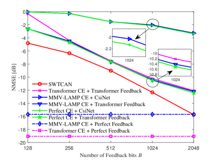
(a) $\rho=8$

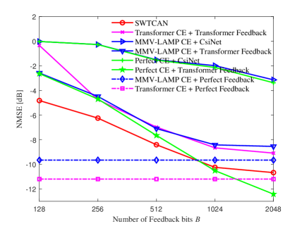
(b) $\rho=16$

Figure 2: NMSE performance of different schemes versus the feedback overhead $B$ for CDL-B.

IV-A Performance of Proposed SWTCAN

We compare the proposed SWTCAN with the following baselines. Baseline 1: The Transformer-based network for CE and CSI feedback [9], denoted as ‘Transformer CE + Transformer Feedback’. Baseline 2: The multiple-measurement-vectors (MMV)-learned approximate message passing (LAMP) algorithm [22] for CE and the bit-level CsiNet scheme with an attention mechanism [23] or a Transformer-based network for CSI feedback, denoted as “MMV-LAMP CE + CsiNet/Transformer Feedback’. Baseline 3: The perfect downlink channel estimate and the bit-level CsiNet scheme with an attention mechanism [23] or a Transformer-based network for CSI feedback, denoted as ‘Perfect CE + CsiNet/Transformer Feedback’. Baseline 4: The MMV-LAMP algorithm or a Transformer-based network for CE and the perfect CSI feedback to the BS, denoted as ‘MMV-LAMP/Transformer CE + Perfect Feedback’.

Fig. 2 shows the NMSE performance achieved by different schemes versus the feedback overhead B. Both the training and test datasets are CDL-B channels. Fig. 2a indicates that at a compression ratio $\rho\!=\!\frac{N_{\rm{BS}}}{M}\!=\!8$, the main factor influencing the performance is the CSI feedback scheme. Our SWTCAN demonstrates excellent performance across all feedback bit numbers B, outperforming the baseline schemes and approaching the performance of perfect CSI feedback at $B\!=\!2048$. Fig. 2b shows that at a higher $\rho\!=\!16$, the CE algorithm also affects the final performance. Simulations on CDL-A and CDL-C channels, not showing due to space limits, also verify the same advantages of our proposed SWTCAN.

IV-B Performance of Proposed Generative Pre-Training

We evaluate the performance of generative pre-training on SWTCAN at $\rho\!=\!8$ and $B\!=\!512$, 1024 and 2048 bits with the value of $l$ in (III-A) set to 0.00025. We assume that the BS has 6000 CDL-A CSI samples, which are obtained from the channel model generator. But the true CSI distribution in the BS’s cell follows a different CDL-B distribution. The BS only has 120 high-quality CDL-B samples, which are obtained from the uplink CE. We compare the proposed scheme and three benchmark schemes for ablation study. Scheme A: We pre-train SWTCAN with 6000 CDL-A samples. Scheme B: We pre-train SWTCAN with 120 CDL-B samples. Scheme C: We train VAE-CSG with 120 CDL-B samples, and then use it to generate 6000 CSI samples to pre-train SWTCAN. By contrast, in the Proposed scheme, we pre-train VAE-CSG with 6000 CDL-A samples, fine-tune it with 120 CDL-B samples, and finally generate 6000 CSI samples to pre-train SWTCAN. These four pre-training schemes are tested on 2000 CDL-B samples, and the pre-training test NMSEs are compared in Table I. It can be seen that the proposed VAE-CSG outperforms the other three benchmark schemes, demonstrating its effectiveness. Based on the proposed pre-training strategy, the performance of SWTCAN at $\rho\!=\!8$ and $B\!=\!2048$ bits reaches the NMSE of -9.3678 dB, which is still a bit short of -15.7 dB shown in Fig. 2a. Therefore, we use federated-tuning to further improve the performance.

TABLE I: Pre-training test NMSE (dB) performance comparison of different pre-training schemes under the CDL-B channel.

Number of feedback bits	Scheme A	Scheme B	Scheme C	Proposed
B=512	0.2009	-2.8306	-4.0628	-5.0361
B=1024	0.2491	-3.7469	-5.5036	-7.3138
B=2048	-0.1258	-3.9417	-6.6860	-9.3678

IV-C Performance of Proposed Federated-Tuning Method

In this ablation study, there are $U\!=\!600$ UEs, each having $N_{\rm FL}^{s}=10$ actual CSI samples. During each communication round of federated-tuning, 10% of UEs, i.e., 60 UEs, are involved, and each UE conducts $K\!=\!2$ local training epochs with the local training rate $\eta_{l}\!=\!0.001$ to facilitate online fine-tuning of SWTCAN at $\rho\!=\!8$ and $B\!=\!2048$ bits. The hyperparameters in (11) are set to $\eta\!=\!1$, $\beta_{1}\!=\!0.9$, and $\beta_{2}\!=\!0.99$. We freeze the parameters of the SWTCAN except for the last two layers in the decoder. SNR is set to 20 dB for both downlink CE and uplink AirComp. For federated-tuning, computation (updating the trainable parameters $\tilde{\bm{\theta}}$) is done in the UE, and the model updates of multiple UEs are transmitted using AirComp. For CL, the BS collects CSI samples via orthogonal transmission, and then updates the whole model parameters $\bm{\theta}$. Note that $|\tilde{\bm{\theta}}|_{c}\!=\!$ 3 617 280, $|\bm{\theta}|_{c}\!=\!$ 32 623 524, hence $|\tilde{\bm{\theta}}|_{c}\approx 0.11|\bm{\theta}|_{c}$.

TABLE II: Characterization of communication overhead, computation cost and computation speed of federated-tuning and CL schemes.

[b] Federated-tuning (one global epoch) CL (one CSI sample) Communication overhead ($\times 10^{5}$ real numbers) $|\tilde{\bm{\theta}}|\approx 36$ $2PN_{\mathrm{BS}}\approx 1.3$ Computation cost ($\times 10^{9}$ FLOPs) $\zeta_{\mathrm{UE}}\approx 2.6$ $\zeta_{\mathrm{BS}}\approx 3.4$ Computational speed (FLOPs/s) $\kappa_{\mathrm{UE}}$ $\kappa_{\mathrm{BS}}=\gamma\kappa_{\mathrm{UE}}$

• The computation cost containing both forward and backward propagations is numerically calculated using torch-summary[24]. Note that federated-tuning and CL have the same forward propagation, while federated-tuning has less computation cost in the backward propagation.

Table II characterizes the communication overhead, computation cost and computation speed of the federated-tuning (one global epoch) and the CL scheme (one CSI sample). For a fair comparison, later we will compare the NMSE performance of the two schemes, given the same communication resources and the same computation time. Here, we first calculate how many CSI samples the BS can collect in CL, given a fixed communication resource. Specifically, consider $T_{0}$ global epochs of federated-tuning, within which period the communication overhead is $T_{0}|\tilde{\bm{\theta}}|_{c}$. Using the same communication resources, the BS in CL can collect $N_{\rm CL}^{s}\!=\!\frac{T_{0}|\tilde{\bm{\theta}}|_{c}}{2PN_{\mathrm{BS}}}$ CSI samples for central training. Furthermore, we calculate how many training epochs CL can have, given a fixed computation time. In particular, given the number of global epochs $T_{0}$, the computation cost $\zeta_{\mathrm{UE}}$, the number of local CSI samples $N_{\rm FL}^{s}$, the number of local training epochs $K$, and the computation speed $\kappa_{\mathrm{UE}}$, the computation time of federated-tuning can be calculated as $\tau\!=\!\frac{T_{0}N_{\rm FL}^{s}K\zeta_{\mathrm{UE}}}{\kappa_{\mathrm{UE}}}$. Within the same computation time $\tau$ in CL, given the computation cost $\zeta_{\mathrm{BS}}$, the number of CSI samples collected in the BS $N_{\rm CL}^{s}$, and the computation speed in the BS $\kappa_{\mathrm{BS}}$, we can obtain the number of training epochs of CL as $K_{\rm CL}\!=\!\frac{\tau\kappa_{\mathrm{BS}}}{N_{\rm CL}^{s}\zeta_{\mathrm{BS}}}$. Note that $\kappa_{\mathrm{BS}}\!=\!\gamma\kappa_{\mathrm{UE}}$. Although the BS is typically computationally more powerful than a UE, i.e., $\gamma>1$, our proposed federated-tuning method still shows advantages due to the collaboration of multiple UEs.

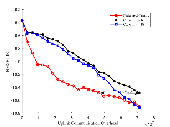
Figure 3: Performance comparison of federated-tuning and CL schemes versus the uplink communication overhead.

Fig. 3 compares the NMSE of the proposed federated-tuning with that of the CL scheme versus uplink communication overhead. It can be seen that our federated-tuning method exhibits superior NMSE performance compared to the CL scheme under the same computation time and the same uplink communication overhead. Specifically, to achieve an equivalent NMSE performance in the same computation time, compared to the CL scheme with $\gamma\!=\!16$ (this situation is possible, e.g., a Nvidia 3090Ti graphics card with a computing power of 41.6 TFLOPs on the BS and an iPad Air with a computing power of 2.6 TFLOPs on the M1 chip of the UE), our proposed algorithm reduces uplink communication overhead by up to 34.8%. For the CL scheme, as the ratio of computational speed $\gamma$ increases, the number of training epochs that BS can conduct also increase given the same computation time, resulting in improved performance.

V Conclusions

We have proposed a Swin Transformer-based CSI acquisition network called SWTCAN to jointly design the pilot, CSI compression and CSI reconstruction. In order to solve the training data scarcity problem as the actual CSI samples are difficult to measure, we have designed the VAE-CSG to generate CSI samples for pre-training SWTCAN. The combination of VAE-CSG and SWTCAN constitutes the downlink CSI acquisition network based on a generative pre-trained Transformer at the BS. To further enhance the performance of the pre-trained SWTCAN, we have utilized the communication-efficient federated-tuning and AirComp to fine-tune the SWTCAN, while substantially reducing uplink communication overhead. Simulations have demonstrated that our proposed SWTCAN has better performance compared to the state-of-the-art schemes, and have verified the communication efficiency of the proposed federated-tuning method.

References

- [1] Z. Gao, L. Dai, Z. Wang, and S. Chen, “Spatially common sparsity based adaptive channel estimation and feedback for FDD massive MIMO,” IEEE Trans. Signal Process., vol. 63, no. 23, pp. 6169–6183, 2015.
- [2] J. Guo, C.-K. Wen, S. Jin, and G. Y. Li, “Overview of deep learning-based CSI feedback in massive MIMO systems,” IEEE Trans. Commun., vol. 70, no. 12, pp. 8017–8045, 2022.
- [3] X. Ma and Z. Gao, “Data-driven deep learning to design pilot and channel estimator for massive MIMO,” IEEE Trans. Veh. Techno., vol. 69, no. 5, pp. 5677–5682, 2020.
- [4] M. B. Mashhadi and D. Gündüz, “Pruning the pilots: Deep learning-based pilot design and channel estimation for MIMO-OFDM systems,” IEEE Trans. Wireless Commun., vol. 20, no. 10, pp. 6315–6328, 2021.
- [5] C.-K. Wen, W.-T. Shih, and S. Jin, “Deep learning for massive MIMO CSI feedback,” IEEE Wireless Commun. Lett., vol. 7, no. 5, pp. 748–751, 2018.
- [6] J. Guo, C.-K. Wen, S. Jin, and G. Y. Li, “Convolutional neural network-based multiple-rate compressive sensing for massive MIMO CSI feedback: Design, simulation, and analysis,” IEEE Trans. Wireless Commun., vol. 19, no. 4, pp. 2827–2840, 2020.
- [7] J. Guo, et al., “Deep learning for joint channel estimation and feedback in massive MIMO systems,” Digital Commun. Netw., vol. 10, no. 1, pp. 83–93, 2024.
- [8] J. Guo, C.-K. Wen, and S. Jin, “CAnet: Uplink-aided downlink channel acquisition in FDD massive MIMO using deep learning,” IEEE Trans. Commun., vol. 70, no. 1, pp. 199–214, 2022.
- [9] Y. Wang, et al., “Transformer-empowered 6G intelligent networks: From massive MIMO processing to semantic communication,” IEEE Wireless Commun., vol. 30, no. 6, pp. 127–135, 2023.
- [10] K. Han, et al., “A survey on vision transformer,” IEEE Trans. Pattern Anal. Mach. Intell., vol. 45, no. 1, pp. 87–110, 2023.
- [11] 3GPP, “Study on channel model for frequencies from 0.5 to 100 GHz,” 3rd Generation Partnership Project (3GPP), Tech. Rep. TR 38.901, May 2017.
- [12] H. Xiao, W. Tian, W. Liu, and J. Shen, “ChannelGAN: Deep learning-based channel modeling and generating,” IEEE Wireless Commun. Lett., vol. 11, no. 3, pp. 650–654, 2022.
- [13] Z. Yang, et al., “Federated learning for 6G: Applications, challenges, and opportunities,” Engineering, vol. 8, pp. 33–41, 2022.
- [14] M. M. Amiri and D. Gündüz, “Federated learning over wireless fading channels,” IEEE Trans, Wireless Commun., vol. 19, no. 5, pp. 3546–3557, 2020.
- [15] J. Chen, et al., “FedTune: A deep dive into efficient federated fine-tuning with pre-trained Transformers,” arXiv preprint arXiv:2211.08025, 2022.
- [16] A. M. Elbir and S. Coleri, “Federated learning for channel estimation in conventional and RIS-assisted massive MIMO,” IEEE Trans. Wireless Commun., vol. 21, no. 6, pp. 4255–4268, 2022.
- [17] L. Dai and X. Wei, “Distributed machine learning based downlink channel estimation for RIS assisted wireless communications,” IEEE Trans. Commun., vol. 70, no. 7, pp. 4900–4909, 2022.
- [18] L. Zhao, et al., “Joint channel estimation and feedback for mm-wave system using federated learning,” IEEE Commun. Lett., vol. 26, no. 8, pp. 1819–1823, 2022.
- [19] Z. Liu, et al., “Swin Transformer: Hierarchical vision Transformer using shifted windows,” in Proc. ICCV 2021, Oct. 11-17, 2021, pp. 10012–10022.
- [20] D. P. Kingma and M. Welling, “Auto-encoding variational Bayes,” arXiv preprint arXiv:1312.6114, 2013.
- [21] Y. Wang, L. Lin, and J. Chen, “Communication-efficient adaptive federated learning,” in Proc. ICML 2022 (Baltimore, MD, USA), Jul. 17-23, 2022, pp. 22802–22838.
- [22] X. Ma, Z. Gao, F. Gao, and M. Di Renzo, “Model-driven deep learning based channel estimation and feedback for millimeter-wave massive hybrid MIMO systems,” IEEE J. Sel. Areas Commun., vol. 39, no. 8, pp. 2388–2406, 2021.
- [23] C. Lu, W. Xu, S. Jin, and K. Wang, “Bit-level optimized neural network for multi-antenna channel quantization,” IEEE Wireless Commun. Lett., vol. 9, no. 1, pp. 87–90, 2020.
- [24] T. Yep, “torch-summary 1.4.5,” https://pypi.org/project/torch-summary/, accessed Dec. 24, 2020.