Non-stationary Spatio-Temporal Modeling Using the Stochastic Advection-Diffusion Equation

Abstract

We construct flexible spatio-temporal models through stochastic partial differential equations (SPDEs) where both diffusion and advection can be spatially varying. Computations are done through a Gaussian Markov random field approximation of the solution of the SPDE, which is constructed through a finite volume method. The new flexible non-separable model is compared to a flexible separable model both for reconstruction and forecasting and evaluated in terms of root mean square errors and continuous rank probability scores. A simulation study demonstrates that the non-separable model performs better when the data is simulated with non-separable effects such as diffusion and advection. Further, we estimate surrogate models for emulating the output of a ocean model in Trondheimsfjorden, Norway, and simulate observations of autonoumous underwater vehicles. The results show that the flexible non-separable model outperforms the flexible separable model for real-time prediction of unobserved locations.

Keywords: Spatio-temporal, non-stationarity, SPDE approach, finite volume method, Gaussian Markov random fields, emulation of numerical models.

1 Introduction

Spatio-temporal data consists of observations that have associated both spatial locations and time points. For example, temperature or precipitation measured at different weather stations, or the concentration of pollutants in the ocean measured from ships. Developing new statistical models for analyzing such data is an active area of research (Porcu et al.,, 2021). The overarching goal is first to accurately capture the complex interactions between space and time in natural phenomena while also enabling efficient computation for handling large datasets. Then, to leverage the estimated interactions to predict unobserved locations or to forecast.

A common approach to model spatio-temporal data is through Gaussian random fields (GRFs); see, for example, Cressie and Wikle, (2011). GRFs are fully characterized by a mean function and a covariance function, which means that the key questions are how to model the mean structure and how to model the covariance structure? However, the covariance function must be positive semi-definite, and this complicates the construction of valid models with realistic features.

A simple way to guarantee a valid spatio-temporal covariance function is to take the product of a spatial covariance function and a temporal covariance function. This is called a separable covariance function but requires a very specific and simple interaction between space and time, and natural processes such as advection and diffusion are non-separable. Typically, one would construct separable covariance functions using stationary and isotropic covariance functions such as the Matérn family of covariance functions, which is popular due to the interpretable parameters and the flexibility in controlling the smoothness, range, and variance. The specification of covariance functions for highly dynamic and non-stationary processes is known to be challenging (Cressie and Wikle,, 2011; Simpson et al.,, 2012), and assumptions such as isotropy, stationarity, and separability are often made to improve computational tractability even though they are physically unrealistic.

Spatio-temporal datasets can be large, and direct computations are limited by a complexity of (${\cal O}(n^{3})$), where $n$ is the number of observations. This is often called the ”big $n$ problem” (Banerjee et al.,, 2003). Many approaches have been suggested to handle large datasets (Heaton et al.,, 2019). Some include include low-rank matrices (Cressie and Johannesson,, 2008; Banerjee et al.,, 2008; Wikle,, 2010), approximate likelihoods (Vecchia,, 1988; Eidsvik et al.,, 2014; Katzfuss and Guinness,, 2021), and Gaussian Markov random fields (GMRFs) (Rue and Held,, 2005). However, an issue with GMRFs is that they are defined through Markov properties and conditional distributions, and are difficult to construct, in general. Lindgren et al., (2011) proposed to overcome this issue by defining models using stochastic partial differential equations (SPDEs) instead of covariance functions, and then constructing GMRFs that approximate the solutions of the SPDEs.

SPDEs are a powerful modeling tool for constructing non-separable spatio-temporal GRFs as they can be related to partial differential equations that describe physical laws. For instance, the stochastic heat or diffusion equation (Heine,, 1955; Jones and Zhang,, 1997; Lindgren et al.,, 2023), the stochastic wave equation (Carrizo Vergara et al.,, 2022), and the stochastic advection-diffusion equation (Liu et al.,, 2022; Clarotto et al.,, 2023). In the context of the SPDE approach, a common way to construct separable covariance structures have been to use an autoregressive process of order 1 (AR(1) process), where the temporal innovations are spatial GRFs (Rodríguez-Iturbe and Mejía,, 1974; Cameletti et al.,, 2013). Spatial non-stationarity can be introduced in the innovations using SPDEs with spatially varying coefficients (Fuglstad et al., 2015a, ; Fuglstad et al., 2015b, ; Hildeman et al.,, 2021; Berild and Fuglstad,, 2023). This gives a separable spatio-temporal covariance structure with spatial non-stationarity (Fuglstad and Castruccio,, 2020).

A promising approach to construct a class of non-separable covariance models with spatial non-stationarity is to start with the stochastic advection-diffusion equation. Previous work has approximated solutions through spectral representations (Sigrist et al.,, 2014; Liu et al.,, 2022), or numerical methods such as finite element methods (FEMs) (Clarotto et al.,, 2023; Lindgren et al.,, 2023). An issue with FEM is that it can be unstable in an advection-dominated setting (Clarotto et al.,, 2023). However, a more natural choice in a conservation law setting is to use the finite volume method (FVM), as it is based on the flow of matter between cells in the discretization, and therefore, the FVM is often closer to the physics of the problem (LeVeque,, 2002). The FVM has been used in Fuglstad et al., 2015a ; Fuglstad et al., 2015b and Berild and Fuglstad, (2023) in a purely spatial setting, but the FVM has not been used in spatio-temporal statistics even though it is prevalent in the field of computational fluid dynamics.

The novel features of this work are: 1) parametrized spatially varying advection and anisotropic diffusion, 2) a non-stationary initial distribution, 3) the use of a FVM discretization of the stochastic advection-diffusion equation, and 4) demonstrating the usefulness of this approach to construct a statistical spatio-temporal surrogate model to a deterministic numerical model. The new class of models allows for a wide range of spatio-temporal behavior to be captured. With such a highly parameterized model, comes the challenge of navigating the likelihood surface for such a high-dimensional parameter space. We show that this is possible by borrowing optimization techniques from the machine learning literature.

The behavior of the ocean is complex, and we need high-resolution deterministic numerical models that are based on the Navier-Stokes equations to describe it well. Such deterministic models are hard to update in real-time due to their computational complexity (Liu et al.,, 2022). In contrast, statistical models are highly effective for space-time interpolation and prediction, making them suitable for real-time applications. The challenge lies in sufficiently describing the complex spatio-temporal behavior. We can take advantage of the complex numerical models to estimate complex statistical surrogate models using the abundance of numerically simulated data. Many authors have employed such an approach to estimate models used in ocean monitoring with AUVs but with some limitations and simplifications. Ge et al., (2023) estimated a purely spatial model through covariance functions for ocean salinity field in 3D and used an adaptive sampling strategy to choose locations for the autonomous underwater vehicles (AUVs) to sample. Foss et al., (2022) used the output from a numerical model to estimate an advection-diffusion model with covariate-based advection and constant isotropic diffusion for monitoring mine tailings in the ocean. Berild et al., (2024) estimated a non-stationary and anisotropic spatial model through the SPDE approach for a 3D ocean salinity field.

In Section 2, we outline the theoretical foundation for spatio-temporal modeling using SPDEs. Then in Section 3 we introduce the proposed method for modeling spatio-temporal data and elaborate on the parameterization of the stochastic advection-diffusion equation. In Section 4, we demonstrate the proposed method on a synthetic dataset with a complex spatio-temporal structure and compare its predictive performance to other spatio-temporal models. In Section 5, we apply our method to emulate a numerical ocean model, simulate an ocean monitoring scenario with AUVs, and compare the accuracy of the proposed model to a non-stationary separable spatio-temporal model. Finally, Section 6 presents a discussion of the results and our conclusions. Some technical details such as the derivation of the numerical solution of the stochastic advection-diffusion equation are deferred to the appendices. The computer code used in this work is available at https://github.com/berild/spdepy.

2 Spatio-temporal modeling with SPDEs

2.1 Non-stationary spatial modelling

The standard SPDE approach can be extended to non-stationary covariance structures through spatially varying coefficients (Lindgren et al.,, 2011, 2022). For a bounded domain of interest $\mathcal{D}\subset\mathbb{R}^{2}$, we follow Fuglstad et al., 2015a ; Fuglstad et al., 2015b and consider the SPDE

$$\left(\kappa(\bm{s})^{2}-\nabla\cdot\mathbf{H}(\bm{s})\nabla\right)u(\bm{s})=\mathcal{W}(\bm{s}),\quad\bm{s}\in\mathcal{D},$$ (1)

where $\kappa(\cdot)$ is a positive function, $\nabla$ is the gradient, and $\mathbf{H}(\cdot)$ is a differentiable spatially varying symmetric positive definite $2\times 2$ matrix, and $\mathcal{W}(\cdot)$ is Gaussian white noise. See Bolin and Kirchner, (2020) for more details on the technical requirements on $\kappa(\cdot)$ and $\mathbf{H}(\cdot)$. We apply zero-flow Neumann boundary conditions,

$$(\mathbf{H}(\bm{s})\nabla u(\bm{s}))\cdot\bm{n}(\bm{s})=0,\quad\bm{s}\in\partial\mathcal{D},$$

where $\partial\mathcal{D}$ is the boundary of $\mathcal{D}$ and $\bm{n}(\cdot)$ is the outwards normal vector on the boundary. This approach can be extended to $\mathbb{R}^{3}$ (Berild and Fuglstad,, 2023) and fractional powers can be used on the operator on the left-hand side to control smoothness (Bolin and Kirchner,, 2020). We write $u(\cdot)\sim\text{WM}(\kappa(\cdot),\mathbf{H}(\cdot))$ to denote that $u(\cdot)$ has the Whittle-Matérn distribution arising from Equation (1) with the no-flow boundary condition, where the dependence on the domain $\mathcal{D}$ is suppressed in the notation.

Consider the stationary case that $\kappa(\cdot)\equiv\kappa_{0}$ and $\mathbf{H}(\cdot)\equiv\mathbf{H}_{0}$, and ignore the boundary effects. Then $u(\cdot)\sim\text{WM}(\kappa_{0},\mathbf{H}_{0})$ leads to a Matérn covariance function

$$c(\bm{s},\bm{s}^{\prime})=\sigma^{2}\left(\kappa_{0}\left\lVert\mathbf{H}_{0}^{-1/2}(\bm{s}-\bm{s}^{\prime})\right\rVert\right)K_{1}\left(\kappa_{0}\left\lVert\mathbf{H}_{0}^{-1/2}(\bm{s}-\bm{s}^{\prime})\right\rVert\right),\quad\bm{s},\bm{s}^{\prime}\in\mathbb{\mathcal{D}},$$ (2)

where $\mathbf{H}_{0}^{-1/2}$ is the inverse of the square root of $\mathbf{H}_{0}$, $\left\lVert\cdot\right\rVert$ is the Euclidean norm, $\sigma^{2}$ is the marginal variance, and $K_{1}$ is the modified Bessel function of the second kind, order $1$. This is an anisotropic Matérn covariance function with smoothness $1$, and as shown in Fuglstad et al., 2015a , the marginal variance is given by

$$\sigma^{2}=1/(4\pi\kappa_{0}^{2}\sqrt{\det\mathbf{H}_{0}}).$$

In practice, the influence of the boundary condition on an area of interest can be reduced by extending the domain $\mathcal{D}$ to cover more than the area of interest (Lindgren et al.,, 2011).

In the case that $\kappa(\cdot)$ and $\mathbf{H}(\cdot)$ are spatially varying, there is no obvious way to avoid boundary effects since there is no unique way to extend $\kappa(\cdot)$ and $\mathbf{H}(\cdot)$ to a larger domain than the area of interest. In practice, one can use a larger domain than the area of interest, and then estimate $\kappa(\cdot)$ and $\mathbf{H}(\cdot)$ also outside the area of interest (Fuglstad et al., 2015b, ). The anisotropic Laplacian in Equation (1) induces local anisotropy in the correlation at every location, and the combination of $\kappa(\cdot)$ and $\mathbf{H}(\cdot)$ controls the spatially varying spatial dependence and spatially varying marginal variance. See the discussion in Fuglstad et al., 2015b .

In this paper, we will follow Fuglstad et al., 2015a and parametrize $2\times 2$ symmetric positive matrices through

$$\mathbf{H}(\bm{s})=\gamma(\bm{s})\mathbf{I}_{2}+{\bm{v}}(\bm{s}){\bm{v}}(\bm{s})^{\top},\quad\bm{s}\in\mathcal{D},$$ (3)

where $\gamma(\cdot)>0$ controls an isotropic baseline dependence, $\mathbf{I}$ is the identity matrix, and ${\bm{v}}(\cdot)$ is a vector field that controls the direction and strength of extra anisotropy at each location. For inference, we then expand $\log(\kappa(\cdot))$, $\log(\gamma(\cdot))$, $v_{1}(\cdot)$, and $v_{2}(\cdot)$ in bases and estimate the coefficients of the basis functions (Fuglstad et al., 2015b, ; Berild and Fuglstad,, 2023). The details are discussed in Section 3.2.

2.2 Separable spatio-temporal modelling

A direct way to extend $\text{WM}(\kappa(\cdot),\mathbf{H}(\cdot))$, to a spatio-temporal GRF is to use a temporal AR(1) process, where the increments are $\text{WM}(\kappa(\cdot),\mathbf{H}(\cdot))$. This gives

$$u^{k+1}(\bm{s})=au^{k}(\bm{s})+\sqrt{1-a^{2}}\phi^{k}(\bm{s}),\quad\bm{s}\in\mathcal{D},\quad k=1,\ldots,K-1,$$ (4)

where $K$ is the number of time steps, $|a|<1$ describes temporal autocorrelation, and $u^{1}(\cdot),\phi^{1}(\cdot),\ldots,\phi^{K-1}(\cdot)\overset{\text{iid}}{\sim}\text{WM}(\kappa(\cdot),\mathbf{H}(\cdot))$. Fuglstad and Castruccio, (2020) used such a construction for a global model with $\mathcal{D}=\mathbb{S}^{2}$, and Cameletti et al., (2013) used this construction with $\kappa(\cdot)\equiv\kappa_{0}\sqrt{\tau}>0$ and $\mathbf{H}(\cdot)\equiv\tau\mathbf{I}$, where $\mathbf{I}$ is the $2\times 2$ identity matrix and $\tau>0$ is a scaling parameter.

Introduce the GRF $\{B(\bm{s},t):\bm{s}\in\mathcal{D},t\in[0,\infty)\}$ such that

1. $B(\cdot,0)\equiv 0$,

2. $B(\cdot,\cdot)$ has independent increments in time, and

3. $(B(\cdot,t_{2})-B(\cdot,t_{1}))/\sqrt{t_{2}-t_{1}}\sim\text{WM}(\kappa(\cdot),\mathbf{H}(\cdot))$ for all $t_{2}>t_{1}\geq 0$.

With an additional technical requirement that the sample paths of $B(\cdot,\cdot)$ are continuous in time, this is an extension of the traditional Brownian motion to a spatio-temporal setting and can be formalized as a Q-Wiener process (Da Prato and Zabczyk,, 2014, p. 81).

Following Lindgren et al., (2022) and using the Q-Wiener process $B(\cdot,\cdot)$, one can view the AR(1) process above as arising from an SPDE

$$\frac{\partial}{\partial t}u(\bm{s},t)+cu(\bm{s},t)=\sqrt{2c}\frac{\partial}{\partial t}B(\bm{s},t),\quad\bm{s}\in\mathcal{D},\quad t\in(0,\infty)$$ (5)

with the initial condition $u(\cdot,0)\sim\text{WM}(\kappa(\cdot),\mathbf{H}(\cdot))$. Equation (4) can be viewed as a discrete approximation of the above SPDE, and the parameter $a$ in Equation (4) depends on $c$ and the temporal resolution used in the approximation.

2.3 The stochastic advection-diffusion equation

A weakness of separable spatio-temporal models is that they cannot include non-separable phenomena such as diffusion and advection. Constructing non-separable spatio-temporal GRFs with spatially varying diffusion and advection through covariance functions is hard, but they are easy to construct through a stochastic advection-diffusion-reaction SPDE. We extend Equation (5) to

$$\frac{\partial}{\partial t}u(\bm{s},t)+\mathrm{A}(\bm{s})u(\bm{s},t)=\tau\frac{\partial}{\partial t}B(\bm{s},t),\quad\bm{s}\in\mathcal{D},\quad t\in(0,\infty),$$ (6)

where $\mathrm{A}(\cdot)$ is discussed in the next paragraph, $\tau>0$ is a scaling parameter, and the Q-Wiener process $B(\cdot,\cdot)$ has increments described through $\text{WM}(\kappa_{\mathrm{F}}(\cdot),\mathbf{H}_{\mathrm{F}}(\cdot))$. The initial condition is $u(\cdot,0)\sim\text{WM}(\kappa_{\mathrm{I}}(\cdot),\mathbf{H}_{\mathrm{I}}(\cdot))$. The subscripts “F” and “I” are short for “Forcing” and “Initial”. The boundary conditions are described in the next paragraph after defining the operator $\mathrm{A}(\cdot)$.

The advection, diffusion, and reaction are described as

$$\mathrm{A}(\bm{s})u(\bm{s},\cdot)=\left(\kappa_{\mathrm{E}}(\bm{s})^{2}-\nabla\cdot\mathbf{H}_{\mathrm{E}}(\bm{s})\nabla\right)u(\bm{s},\cdot)+\nabla\cdot(\bm{\omega}_{\mathrm{E}}(\bm{s})u(\bm{s},\cdot)),\quad\bm{s}\in\mathcal{D},$$

where $\kappa_{\mathrm{E}}(\bm{s})^{2}u(\bm{s},\cdot)$ specifies dampening, $\nabla\cdot\mathbf{H}_{\mathrm{E}}(\bm{s})\nabla u(\bm{s},\cdot)$ specifies anisotropic diffusion, and $\nabla\cdot(\bm{\omega}_{\mathrm{E}}(\bm{s})u(\bm{s},\cdot)$ specifies advection. This means that $\kappa_{\mathrm{E}}(\cdot)$ is a positive function, $\mathbf{H}_{\mathrm{E}}(\cdot)$ is a differentiable spatially varying positive definite $2\times 2$ matrix, and $\bm{\omega}_{\mathrm{E}}(\cdot)$ is a differentiable vector field. The subscript E is short for “Evolution”. We use zero flow boundary conditions given by

$$\left(\mathbf{H}_{\mathrm{E}}(\bm{s})\nabla u(\bm{s},t)+\bm{\omega}_{\mathrm{E}}(\bm{s})u(\bm{s},t)\right)\cdot{\bm{n}}(\bm{s})=0,\quad\bm{s}\in\partial\mathcal{D},\quad t\in(0,\infty),$$ (7)

where ${\bm{n}}(\cdot)$ is the outwards normal vector at the boundary. To reduce the flexibility, we set $\kappa_{\mathrm{F}}(\cdot)=\kappa_{\mathrm{E}}(\cdot)$ and $\mathbf{H}_{\mathrm{F}}(\cdot)\equiv\mathbf{I}$ for the increments in $B(\cdot,\cdot)$. This means that the coefficients to set or to estimate are $\kappa_{\mathrm{E}}(\cdot)$, $\mathbf{H}_{\mathrm{E}}(\cdot)$, $\bm{\omega}_{\mathrm{E}}(\cdot)$, $\tau$, $\kappa_{I}(\cdot)$, and $\mathbf{H}_{\mathrm{I}}(\cdot)$.

Other boundary conditions that could be considered for Equation (6) are Dirichlet boundary conditions given by

$$u(\bm{s},t)=0,\quad\bm{s}\in\partial\mathcal{D},\quad t\in(0,\infty).$$ (8)

Additionally, for a rectangular domain, we could consider periodic boundary conditions where the left-hand side and right-hand side are identified, and the bottom side and top side are identified. In this context, this means that what flows out on one side of the domain flows in on the other side.

3 Modeling spatial-temporal data

3.1 Latent model and observation model

We consider a bounded spatial domain $\mathcal{D}\subset\mathbb{R}^{2}$ and a bounded temporal interval $\mathcal{T}\in\mathcal{T}$, and model the latent signal as

$$\eta(\bm{s},t)=\bm{x}(\bm{s},t)^{\mathrm{T}}\bm{\beta}+u(\bm{s},t),\quad\bm{s}\in\mathcal{D},\quad t\in\mathcal{T},$$

where $\bm{x}(\cdot,\cdot)$ is a spatio-temporally varying $p$-dimensional covariate vector, $\beta$ is a $p$-dimensional coefficient vector, and $u(\cdot,\cdot)$ is the advection-diffusion-reaction model discussed in Section 2.3. The parameters controlling $u(\cdot,\cdot)$ are discussed in Section 3.2.

We assume $n$ measurements, $y_{1},\dots,y_{n}\in\mathbb{R}$, are collected at spatial locations $\bm{s}_{1},\ldots,\bm{s}_{n}\in\mathcal{D}$ at times $t_{1},\ldots,t_{n}\in\mathcal{T}$. The observation model is

$$y_{i}=\eta(\bm{s}_{i},t_{i})+\epsilon_{i},\quad i=1,\ldots,n,$$ (9)

where $\epsilon_{1},\ldots,\epsilon_{n}\overset{\text{iid}}{\sim}\mathcal{N}(0,\sigma_{n}^{2})$ with nugget variance $\sigma_{n}^{2}>0$.

3.2 Parametrizing the advection-diffusion-reaction model

The model described in Section 2.3 has coefficients $\kappa_{\mathrm{E}}(\cdot)$, $\mathbf{H}_{\mathrm{E}}(\cdot)$, $\bm{\omega}_{\mathrm{E}}(\cdot)$, $\tau$, $\kappa_{I}(\cdot)$, and $\mathbf{H}_{\mathrm{I}}(\cdot)$. Using the decomposition Equation in (3) on $\mathbf{H}_{\mathrm{E}}(\cdot)$ and $\mathbf{H}_{\mathrm{I}}(\cdot)$, we have one real number controlling the strength of the forcing, $\log(\tau)$, and 10 real functions controlling

• Evolution: $\log(\kappa_{\mathrm{E}}(\cdot))$, $\log(\gamma_{\mathrm{E}}(\cdot))$, $v_{\mathrm{E},1}(\cdot)$, $v_{\mathrm{E},2}(\cdot)$, $\omega_{\mathrm{E},1}(\cdot)$, and $\omega_{\mathrm{E},2}(\cdot)$

• Initial condition: $\log(\kappa_{\mathrm{I}}(\cdot))$, $\log(\gamma_{\mathrm{I}}(\cdot))$, $v_{\mathrm{I},1}(\cdot)$, and $v_{\mathrm{I},2}(\cdot)$.

The $\log$-transformation has been used for all quantities that must be positive.

This means that if we have constant coefficients, there are in total 11 parameters controlling the stochastic advection-diffusion-reaction. If we need spatially varying coefficients, we expand all 10 functions in spline function bases. Specifically, in this paper, we use three 2nd-order B-spline basis functions covering each spatial dimension. Then, combine using tensor product splines as

$$f_{ij}(\bm{s})=B_{x,i}(x)B_{y,j}(y),\quad\mathrm{for}\enspace i=1,2,3\enspace\mathrm{and}\enspace j=1,2,3,$$ (10)

where $B_{x,i}(x)$ and $B_{y,j}(y)$ are the 2nd-order B-spline basis functions in the $x$ and $y$ directions, respectively. A visualization of the B-spline basis functions is shown in Figure 1. This is similar to the approach taken by Fuglstad et al., 2015b and Berild and Fuglstad, (2023) on the Whittle-Matérn SPDE. This gives in total 90 coefficients for the basis functions, and thus 91 parameters including $\log(\tau)$. In general, one could use an arbitrary number of B-spline basis functions in each dimension at the cost of increased computation time. We refer readers to Berild and Fuglstad, (2023, Appendix A.3) for a detailed description of the construction of 1D clamped B-splines.

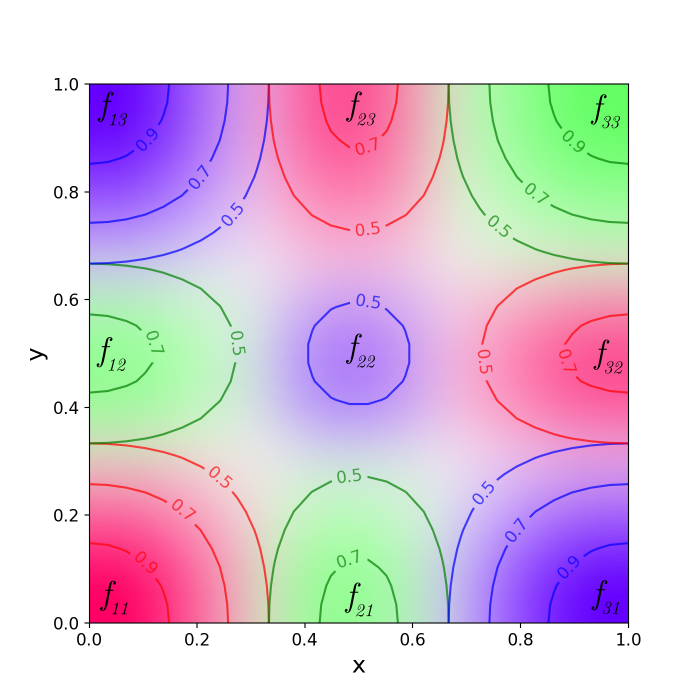
Figure 1: B-spline basis functions for a 2D domain. The colors indicate the value of each basis function, with different colors used solely to distinguish between the functions.

We denote the parameter vector as $\bm{\theta}$, and the vector contains $\log(\tau)$ and all coefficients of basis functions. When $\bm{\theta}$ is known, all functions are known, and the stochastic advection-diffusion-reaction is fully specified. Before we state the full hierarchical model and discuss computations, we discretize the stochastic advection-diffusion-reaction model in space and time.

3.3 Discretizing the advection-diffusion-reaction model

We solve advection-diffusion-reaction SPDE given in Equation (6) numerically by first discretizing in time by backward Euler, and then in space using a finite volume method.

We use a regular sequence of time points $0=t_{0}^{\mathrm{G}}<t_{1}^{\mathrm{G}}<\ldots<t_{T-1}^{\mathrm{G}}$, where the time step is $\Delta t$. Backward Euler for Equation (6) gives

$$(1+\Delta t\mathrm{A}(\cdot))u^{n+1}(\cdot)=u^{n}(\cdot)+\tau(B^{n+1}(\cdot)-B^{n}(\cdot)),\quad n=0,\ldots,T-2,$$ (11)

where $u^{n}(\cdot)=u(\cdot,t_{n}^{\mathrm{G}})$ and $B^{n}(\cdot)=B(\cdot,t_{n}^{\mathrm{G}})$ for $n=0,\ldots,T-1$, and $u^{0}(\cdot)$ follows the initial condition $\text{WM}(\kappa_{\mathrm{I}}(\cdot),\mathbf{H}_{\mathrm{I}}(\cdot))$. Note that

$$(B^{1}(\cdot)-B^{0}(\cdot))/\sqrt{\Delta t},\ldots,(B^{T-1}(\cdot)-B^{T-1}(\cdot))/\sqrt{\Delta t}\overset{\text{iid}}{\sim}\text{WM}(\kappa_{E}(\cdot),\mathbf{I})$$

due to the restriction on the forcing made in Section 2.3.

The spatial domain ${\cal D}$ is subdivided into $K$ regular rectangular grid cells, each represented by a centroid $\bm{s}_{k}$. We assume a piece-wise constant solution with constant value within each grid cell, as is common in standard FVM. A visualization of the spatial discretization is presented in Figure S1. We refer to Appendix A. for technical details and give an overall description of the results below.

Let the discrete approximation of the solution at time $t_{n}$ be denoted by

$${\bm{w}}^{n}=\begin{bmatrix}u^{n}(\bm{s}_{1}),\ldots,u^{n}(\bm{s}_{K})\end{bmatrix}^{\mathrm{T}},\quad n=0,\ldots,T-1.$$

We can then discretize Equation (11) in space as

$$\left(\mathbf{D}_{\mathrm{V}}+\Delta t\left(\mathbf{D}_{\mathrm{V}}\mathbf{D}_{\kappa^{2}}-\mathbf{A}_{\mathbf{H}}+\mathbf{A}_{\bm{\omega}}\right)\right){\bm{w}}^{n+1}=\mathbf{D}_{\mathrm{V}}{\bm{w}}^{n}+\tau\sqrt{\Delta t}\mathbf{D}_{\mathrm{V}}\bm{\phi}^{n},$$ (12)

for $n=0,\ldots,T-2$. Here, $\bm{\phi}^{0},\ldots,\bm{\phi}^{T-2}\overset{\text{iid}}{\sim}\mathcal{N}(\bm{0},\mathbf{Q}_{\mathrm{F}}^{-1})$, where $\mathbf{Q}_{\mathrm{F}}$ is a sparse matrix that arises from a discretization of $\text{WM}(\kappa_{\mathrm{E}}(\cdot),\mathbf{I}_{2})$ using the method described in Fuglstad et al., 2015a . Further, the initial state, ${\bm{w}}^{0}$, is independent of $\bm{\phi}^{0},\ldots,\bm{\phi}^{T-2}$, and $\bm{w}^{0}\sim\mathcal{N}(\bm{0},\mathbf{Q}_{\mathrm{I}})$, where $\mathbf{Q}_{\mathrm{I}}$ is a sparse matrix that arises from a discretization of $\text{WM}(\kappa_{\mathrm{I}}(\cdot),\mathbf{H}_{\mathrm{I}}(\cdot))$ using the method described in Fuglstad et al., 2015a . The matrices are

• $\mathbf{D}_{\mathrm{V}}=V\mathbf{I}_{K}$: a diagonal matrix containing the areas of the cells;

• $\mathbf{D}_{\kappa^{2}}$ and $\mathbf{A}_{\mathrm{H}}$ provide dampening and diffusion, respectively, and are discussed in Fuglstad et al., 2015a (, Appendix A.3);

• $\mathbf{A}_{\bm{\omega}}$: uses an up-wind scheme for advection and details are provided in Appendix A..

3.4 Discrete hierarchical model

Let $\bm{y}=(y_{1},\dots,y_{n})^{\mathrm{T}}$ be the observations in Section 3.1 at locations $\bm{s}_{1},\dots,\bm{s}_{n}\in\mathcal{D}$ and times $t_{1},\dots,t_{n}\in\mathcal{T}$. Let

$${\bm{w}}=\begin{bmatrix}{\bm{w}}^{0}\\ \vdots\\ {\bm{w}}^{T-1}\end{bmatrix}$$

be the vector of the discrete solution of the stochastic advection-diffusion-reaction equation at all time grid points. For ease of description, we assume that all observation time points match one of the time grid points. I.e., $\{t_{1},\ldots,t_{n}\}\subset\{t_{0}^{\mathrm{G}},\ldots,t_{T-1}^{\mathrm{G}}\}$. In the simulation study and the application, this will always be the case.

We can then write the model in vector form,

$$\bm{y}=\mathbf{X}\bm{\beta}+\mathbf{E}{\bm{w}}+\bm{\epsilon},$$ (13)

where $\mathbf{X}$ is a design matrix of the covariates, where each row $i$ is $\bm{x}(\bm{s}_{i},t_{i})^{\mathrm{T}}$, $\bm{\beta}$ is the coefficients of the covariates, $\bm{\epsilon}\sim{\cal N}(\bm{0},\sigma^{2}_{n}\mathbf{I})$, and $\mathbf{E}$ is a $n\times KT$ matrix that selects the correct grid cell in the correct time grid point for each observation. Note that $\mathbf{E}$ has exactly one $1$ on each row and all other elements are $0$.

We introduce a Gaussian penalty $\bm{\beta}\sim{\cal N}\left(\bm{0},V_{\beta}\mathbf{I}\right)$, where $V_{\beta}>0$ is a fixed number, so that the full hierarchical model is

Stage 1: $$\bm{y}\mid\bm{\beta},{\bm{w}},\sigma_{n}^{2}\sim{\cal N}\left(\mathbf{X}\bm{\beta}+\mathbf{E}{\bm{u}},\sigma_{n}^{2}\mathbf{I}\right)$$

Stage 2: $${\bm{w}}\mid\bm{\theta}\sim{\cal N}(\bm{0},\mathbf{Q}^{-1})\enspace,\quad\bm{\beta}\sim{\cal N}\left(\bm{0},V_{\beta}\mathbf{I}\right),$$

where details about $\mathbf{Q}$ is given in Appendix A.. Since ${\bm{w}}$ and $\beta$ are jointly Gaussian given $\bm{\theta}$, we collect them together as ${\bm{z}}=[{\bm{w}},\bm{\beta}]$, and also let $\mathbf{S}=[\mathbf{E},\mathbf{X}]$ such that the hierarchical model becomes

Stage 1: $$\bm{y}\mid{\bm{z}},\sigma_{n}^{2}\sim{\cal N}\left(\mathbf{S}{\bm{z}},\sigma_{n}^{2}\mathbf{I}\right)$$

Stage 2: $${\bm{z}}\mid\bm{\theta}\sim{\cal N}\left(\begin{bmatrix}\bm{0}\\ \bm{0}\end{bmatrix},\begin{bmatrix}\mathbf{Q}^{-1}&0\\ 0&V_{\beta}\mathbf{I}\end{bmatrix}\right)$$

If the parameters $\bm{\theta}$ and $\sigma_{n}^{2}$ are known, then the conditional distribution of the latent field is

$${\bm{z}}|\bm{y},\bm{\theta},\sigma_{n}^{2}\sim\mathcal{N}(\bm{\mu}_{\mathrm{C}},\mathbf{Q}_{\mathrm{C}}^{-1}),$$ (14)

with the conditional precision matrix

$$\mathbf{Q}_{\mathrm{C}}=\mathbf{Q}+\mathbf{S}^{\top}\mathbf{S}\sigma^{-2}_{n},$$ (15)

and the conditional expectation

$$\bm{\mu}_{\mathrm{C}}=\mathbf{Q}_{\mathrm{C}}^{-1}\mathbf{S}^{\top}\bm{y}\sigma^{-2}_{n}.$$ (16)

Using this conditional distribution, the point prediction for an unobserved location $\bm{s}^{*}\in\mathcal{D}$ is given by

$$\mathbb{E}\left[\bm{y}^{*}|\bm{y},\sigma_{n}^{2},\bm{\theta}\right]=\mathbf{S}_{\mathrm{P}}\bm{\mu}_{\mathrm{C}},$$

where $\mathbf{S}_{\mathrm{P}}$ is the corresponding design matrix for the prediction location. The predictive distribution $\bm{y}^{*}|\bm{y},\sigma_{n}^{2},\bm{\theta}$ is Gaussian, and the variance can be found either through algorithms that compute a partial inverse of $\mathbf{Q}_{\mathrm{C}}$ (Rue and Held,, 2010) or estimated through simulation. When forecasts are desired, one includes additional time steps in the discretization that are unobserved, and use the same approach as above.

3.5 Parameter inference

The parameters of the models are inferred using maximum likelihood estimation (MLE) or maximum a posteriori probability (MAP) estimation. The log-posterior (or log-likelihood) is given by

$$\log\pi(\bm{\theta},\sigma^{2}_{n}|\bm{y}) =\mathrm{Const}+\log\pi(\bm{\theta},\sigma^{2}_{n})+\frac{1}{2}\log|\mathbf{Q}_{z}|-\frac{1}{2}\log|\mathbf{Q}_{\mathrm{C}}|+$$ (17)

$$\phantom{=}-\frac{n}{2}\log\sigma^{2}_{n}-\frac{1}{2}\bm{\mu}_{\mathrm{C}}^{\mathrm{T}}\mathbf{Q}_{z}\bm{\mu}_{\mathrm{C}}-\frac{1}{2\sigma^{2}_{n}}(\bm{y}-\mathbf{S}\bm{\mu}_{\mathrm{C}})^{\top}(\bm{y}-\mathbf{S}\bm{\mu}_{\mathrm{C}}),$$

where

$$\mathbf{Q}_{z}=\begin{bmatrix}\mathbf{Q}&0\\ 0&\mathbf{I}/V_{\beta}\end{bmatrix},$$

and we use $\pi(\bm{\theta},\sigma_{n}^{2})\propto 1$ in this paper since we are emulating densely observed numerical model output and do not need extra regularization. For the derivation of the log-likelihood, we refer the reader to Berild and Fuglstad, (2023, Appendix A.4).

Inference is done using some optimization algorithm on the log-posterior to find the parameters that maximize it. To aid the optimization, the gradient of the log-posterior is often used. However, calculating the analytic gradient of the log-posterior requires calulcating $\mathrm{Tr}((\mathbf{Q}_{z}^{-1}-\mathbf{Q}_{\mathrm{C}}^{-1})\frac{\partial\mathbf{Q}_{z}}{\partial\theta_{i}})$ where $\mathrm{Tr}(\cdot)$ denotes the trace of the matrix. Calculation of the inverse of the precision matrices can be avoided by computing a partial inverse only for the non-zero elements (Rue and Held,, 2010), but it is still quite computationally expensive. An alternative, to speed up computations further, is to use the Hutchinson estimator (Hutchinson,, 1990) which is a stochastic approximation of the trace of the matrix,

$$\mathrm{Tr}(\mathbf{A})=\mathbb{E}\left[\bm{\xi}^{\top}\mathbf{A}\bm{\xi}\right]\approx\frac{1}{n}\sum_{i=1}^{n}\bm{\xi}_{i}^{\top}\mathbf{A}\bm{\xi}_{i},$$

where $\bm{\xi}_{i}$ are independent samples from the Rademacher distribution, i.e., $\bm{\xi}_{i}=\pm 1$ with equal probability. This is much faster since it only requires $n$ matrix-vector products and solves, but it makes the optimization problem stochastic.

The drawback of stochastic optimization is that the gradient is noisy, and this can lead to erratic behavior in the optimization, but it is often used because the computational speedup is so significant that the convergence is still faster. There is a vast literature on stochastic gradient methods, and we refer the reader to Ruder, (2017) for an overview. Many of these methods tackle the problem of noisy gradients and use techniques such as momentum, adaptive learning rates, and averaging of gradients to reduce the noise. In this work, we use the Adam optimizer (Kingma and Ba,, 2017) which is a popular choice for optimization of neural networks and other large models.

4 Example: reconstruction and forecasting

In this section, we investigate the ability to reconstruct and forecast a complex process for models of varying degrees of complexity.

4.1 True process and observation model

Consider a spatial domain $\mathcal{D}=[0,15]^{2}$ and temporal domain $\mathcal{T}=[0,2]$. We use a regular discretization with $M=50$ grid cells in $x$-direction, $N=50$ grid cells in $y$-direction, and $T=12$ timesteps. The true process has spatially varying advection and spatially varying anisotropic diffusion. The advection vector field is

$$\bm{\omega}(\bm{s})=30\begin{bmatrix}\sin\left((x/15+1/2)\pi/3\right)\cos\left((y/15+1/2)\pi/3\right)\\ -\cos\left((x/15+1/2)\pi/3\right)\sin\left((y/15+1/2)\pi/3\right)\end{bmatrix},\quad\bm{s}\in\mathcal{D},$$ (18)

and the diffusion matrix is given by $\mathbf{H}(\cdot)=\exp(-1)\mathbf{I}+{\bm{v}}(\cdot){\bm{v}}(\cdot)^{\mathrm{T}}$, where

$${\bm{v}}(\bm{s})=0.7\begin{bmatrix}-\cos\left((x/15+1/2)\pi/3\right)\sin\left((y/15+1/2)\pi/3\right)\\ -\sin\left((y/15+1/2)\pi/3\right)\cos\left((x/15+1/2)\pi/3\right)\end{bmatrix},\quad\bm{s}\in\mathcal{D}.$$ (19)

Here, the vector fields are scaled with a factor of $30$ and $0.7$, respectively, which gives a true process dominated by advection. A visualization of the unscaled vector fields is given in Figure 2, where the length of the vectors shows the magnitude of the fields.

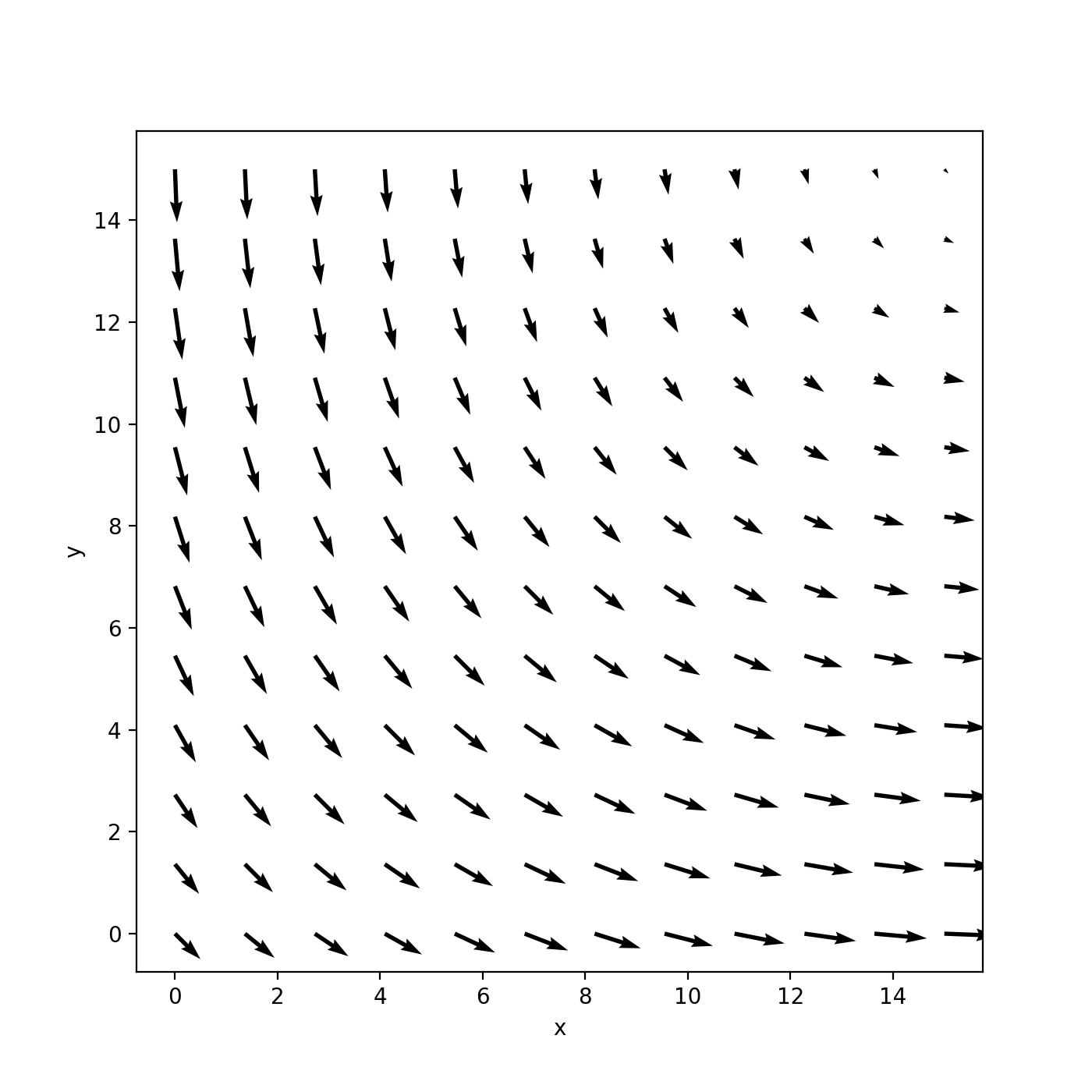
(a) Advection

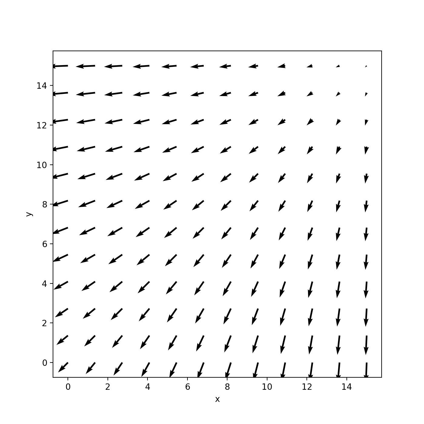
(b) Extra diffusion

Figure 2: The unscaled vector fields describing (a) advection, and (b) extra anisotropic diffusion. The length of the vectors shows the magnitude of the field.

For simplicity, the dampening coefficient is constant $\kappa(\cdot)\equiv\exp(-2)$, the isotropic diffusion parameter is $\gamma(\cdot)\equiv\exp(-1)$, and the scaling parameter for the forcing is $\tau=\exp(-4)$. This defines the true spatio-temporal process $\{u_{\mathrm{true}}(\bm{s},t):\bm{s}\in\mathcal{D},t\in\mathcal{T}\}$, which we call NStat-True. The boundaries of the spatial domain are set to have zero flow going in or out of the domain. Furthermore, in order to reduce the effect of the boundary conditions, a buffer of $5$ grid cells is added to each side of the domain $\mathcal{D}$ resulting in a new domain $\mathcal{D}_{\mathrm{B}}$ of $M=60$ and $N=60$ grid cells. We also apply an advection tapering within this buffer, where the advection vector field is scaled linearly to zero from the boundary of $\mathcal{D}$ to the boundary of $\mathcal{D}_{\mathrm{B}}$. This is to avoid strong advection that suddenly stops at the boundary and inflates marginal variances strongly.

The field can be viewed as the spatio-temporal effect of the concentration of a pollutant in a fluid, where the pollutant is advected by the fluid with a favorable diffusion direction perpendicular to the advection direction. The observation model in this study consists of a spatio-temporal effect observed with random noise. Thus, Equation (9) is simplified to

$$y_{i}=u_{\mathrm{true}}(\bm{s}_{i},t_{i})+\epsilon_{i},\quad\epsilon_{i}\sim\mathcal{N}(0,\sigma_{n}^{2})\quad\forall i.$$ (20)

Here, the noise is i.i.d. Gaussian with variance $\sigma_{n}^{2}=0.001$. Figure 3 shows one realization, marginal variance, and spatio-temporal correlation with the marked location.

The missing rectangle of data is discussed in the next subsection. Here, we observe the correlation move with the advection through time, and with a slight diffusive effect. We can also see an advective effect in the realization, where higher or lower values areas are moved through space with time. The marginal variance shows that the field is not stationary and it is highest at the entry point of the advection vector field, and also the variance changes through time because the initial field does not have the same variance as the field at the end.

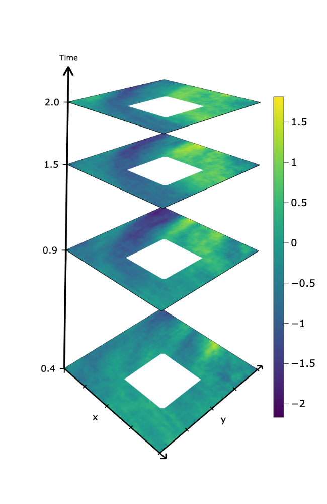
(a) Realization

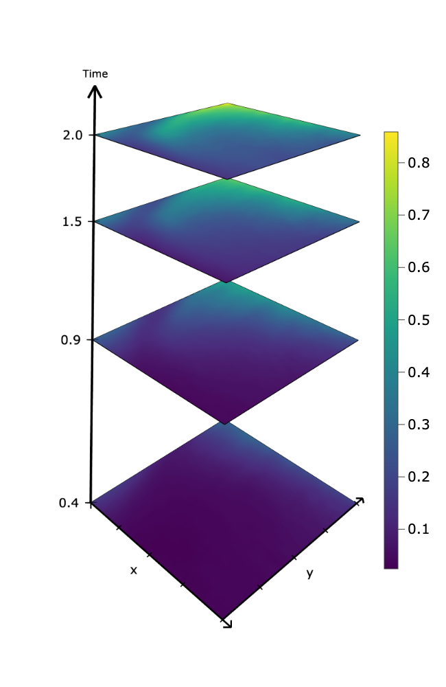
(b) Variance

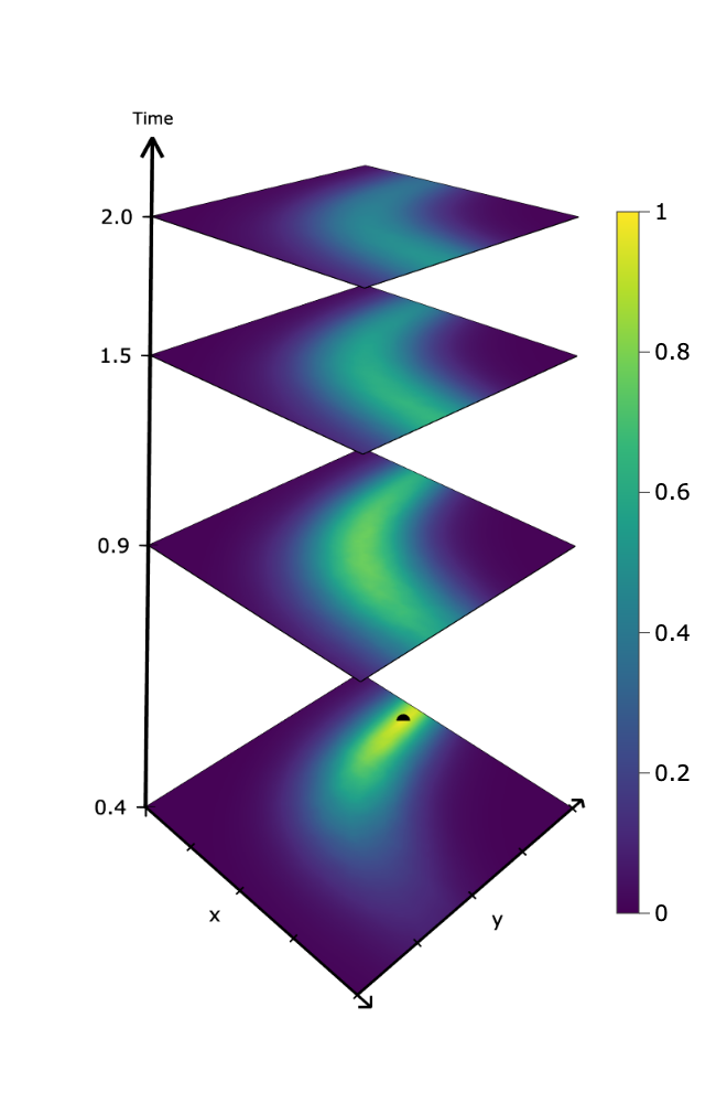
(c) Correlation

Figure 3: Visualization of the model used to simulate the data.

4.2 Goals, and training and test data

We aim to mimic the emulation of a numerical model that is densely observed with a high signal-to-noise ratio. From NStat-True, we observe all grid cells except the grid cells in the rectangle $[6.1,11.6]\times[3.7,9.5]\subset\mathcal{D}$ (rounded to the first decimal), to assess the ability to reconstruct the missing rectangle using data up to the given time, and to forecast for different lags forward in time. The observed grid cells are observed with i.i.d. Gaussian measurement noise with nugget variance $\sigma_{n}^{2}=0.001$.

We generate $20$ realization of the NStat-True for training data that excludes the rectangular area and $20$ realization for the test data that is containing the rectangular area. The training data is demonstrated in Figure 3a. We aim to assess accuracy in reconstructing the masked area from the surrounding observations, and accuracy in forecasting the entire field for different lags forward in time. Let a point prediction for location $\bm{s}_{i}$ be denoted $\hat{y}^{*}_{i,j}=\mathbb{E}[y^{*}_{i}|\bm{y}_{j},\hat{\sigma_{n}^{2}},\hat{\bm{\theta}}]$, where $\bm{y}_{j}$ is the observed data of the $j$th test set, and $\hat{\sigma_{n}^{2}}$ and $\hat{\bm{\theta}}$ are the estimated model parameters. Point predictions are evaluated using root mean square error (RMSE)

$$\mathrm{RMSE}(\Delta k_{p},j)=\sqrt{\frac{1}{n}\sum_{i=1}^{n}\left(y_{i}^{*}-\hat{y}^{*}_{i,j}\right)^{2}},$$

where $n$ is the number of prediction location and $\Delta k_{p}=k_{p}-k_{o}\in\{0,1,2,\ldots,11\}$ is the difference in between predicted $k_{p}$ and observed $k_{o}$ timesteps where $k_{o},k_{p}\in\{1,2,\ldots,12\}$. We also assess the predictive distributions using the continuous ranked probability score (CRPS, Gneiting and Raftery, (2007))

$$\mathrm{CRPS}(\Delta k_{p},j)= \frac{1}{n}\sum_{i=1}^{n}\sigma_{i,j}(z_{i,j}(2\Phi(z_{i,j})-1)+2\phi(z_{i,j})-\pi^{-1/2}),\quad\textrm{for}$$

$$z_{i,j}= \frac{y_{i}^{*}-\hat{y}^{*}_{i,j}}{\sigma_{i,j}},$$

where $\sigma_{i,j}$ is the standard deviation of the predictive distribution $\mathrm{Var}(y^{*}_{i}|\bm{y}_{-j},\hat{\sigma_{n}^{2}},\hat{\bm{\theta}})$, $\Phi(\cdot)$ is the cumulative distribution function of the standard normal distribution, and $\phi(\cdot)$ is the density function of the standard normal distribution. Statistics, such as the average and standard deviation, for these metrics are calculated for each $\Delta k_{p}$ and candidate model over all $j=1,2,\ldots,20$ realizations in the test data.

4.3 Candidate models

We consider four models:

• NStat-True: The true covariance structure;

• NStat-AD: Stochastic advection-diffusion-reaction model discussed in Section 3 with 91 parameters to control covariance and 1 parameter for the nugget variance;

• NStat-Sep: Separable model in Section 2.2 with 37 parameters that control the covariance and 1 parameter for the nugget variance;

• Stat-AD: Stochastic advection-diffusion-reaction model discussed in Section 3 with spatially constant coefficients (11 parameters to control covariance) and 1 parameter for the nugget variance.

NStat-True gives the benchmark for how well we can do, NStat-AD is a flexible model that we believe can capture the non-separability and non-stationarity well, NStat-Sep is a separable model which includes non-stationarity, and Stat-AD is a simplified non-separable model with spatially constant behaviour.

In all models, the mean structure is assumed to be zero with observation model similar to Equation  (20), but replacing $u_{\mathrm{true}}$ with the spatio-temporal effect of each respective model.

4.4 Results

The results are shown in Figure 4. Here, the $x$-axis shows the difference between the timestep when data is observed and the time step when predictions are made $\Delta k_{p}=k_{p}-k_{o}$, where $k_{o}$ is the observed timestep and $k_{p}$ is the prediction timestep. Observations at $k_{o}$ are collected at all locations except the masked area, and predictions are made for all locations at $k_{p}$, except if $k_{p}=k_{o}$, then predictions are made only for the masked area. In Figure 4, the reconstruction error is shown for $\Delta k_{p}=0$ and the forecasting error is for $\Delta k_{p}>0$. For instance, for our timeseries which consist of $12$ timesteps, consider we observe all locations except the masked area at the third timestep ($k_{2}$). Then, the reconstruction is made for the masked area at $k_{2}$ and predictions are made for all locations in the nine future timesteps $0<\Delta k_{p}\leq 9$. In Figure 4, this is added to the evaluation metrics for prediction timesteps $0\leq\Delta k_{p}\leq 9$. If $k_{o}=0$ is observed then $k_{p}=[0,11]$, and if $k_{o}=11$ is observed then only the reconstruction error for $k_{p}=11$ is calculated and errors added to prediction timestep $\Delta k_{p}=0$. This is done for each of the models and an average is taken over the respective $\Delta k_{p}$ made from all combinations of $k_{o}$ and $k_{p}$ and the $20$ realizations in the test data.

First, we remark that NStat-AD has a very close fit to NStat-True, and their error curves are almost identical. Further, all models perform relatively well in reconstructing the masked area, but NStat-AD shows slight improvements over the other models in both RMSE and CRPS. However, we can observe that the standard deviations are larger for reconstruction than for forecasting one timestep ahead. This could be expected as the reconstruction error only considers the masked area, while the forecasting error considers the entire field. The major difference is seen in the forecasting accuracy, already in the first timestep. NStat-Sep is quite good in reconstruction, but the forecasting accuracy is poor. This is reasonable as its spatial covariance structure is flexible, but it is unable to capture the strong advection present in the data-generating model. NStat-Ad is better at forecasting than NStat-Sep. This is expected as it can approximate parts of the advection even though it cannot capture the spatially varying advection. Based on Figure 2(a), it is reasonable that a constant advection vector field could partially approximate the advection vector field.

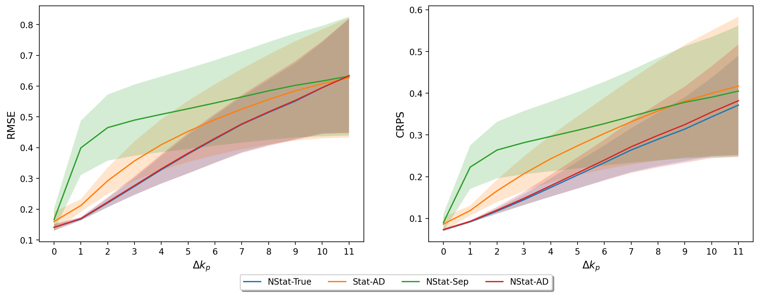
Figure 4: Root mean square error (left) and continuous ranked probability score (right) for the reconstruction ($\Delta k_{p}=0$) and forecasting ($\Delta k_{p}>0$) of the different models.

5 Emulating a numerical ocean model

In this section, we evaluate the proposed approach for simulated AUV paths using numerical ocean model output.

5.1 Motivation and goal

In this case study, we consider output from the SINMOD ocean model (Slagstad and McClimans,, 2005) developed by SINTEF Ocean. The SINMOD ocean model is a 3D numerical model assembled by primitive equations of fluids driven by atmospheric forces, freshwater input, and tides, that is solved using finite difference methods on a regular horizontal grid of cell sizes 20km x 20km which is nested in several steps down to a minimum of 32m x 32m. The temporal resolution is 10 minutes and the depth layers are set specific to a problem but often with higher resolution close to the surface to better capture the variability. The model deals with many ocean quantities such as temperature and currents.

The objective is to estimate a statistical emulator that captures the spatio-temporal variations in the salinity field of a specific area of the Nidelva River outlet in Trondheim, Norway, by utilizing output from the SINMOD model for one specific day (May 27, 2021). This emulator will then be used to predict and forecast salinity levels based on sparse measurements collected by a simulated AUV moving through the SINMOD data from other days than the day used in the estimation of the emulator. By applying the emulator to different days for estimation and prediction, we aim to assess its ability to adapt to varying conditions and simulate the transition from a controlled, simulated environment to less predictable real-world ocean conditions. We choose to consider time segments of 90 minutes which is a typical duration of AUV missions, and we want to be able to forecast within this same time frame.

Figure 5 shows three time segments of 90 minutes on May 27, 2021. The Nidelva River outlet is located in the left corner in the figure or south direction in the area of interest. Here, we can clearly observe the freshwater input from the river and spatio-temporal variations in the salinity field.

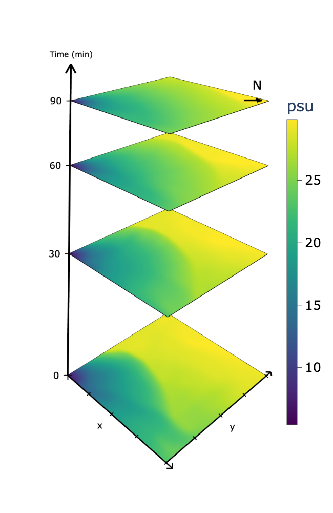
(a)

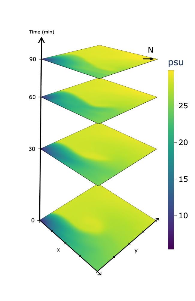
(b)

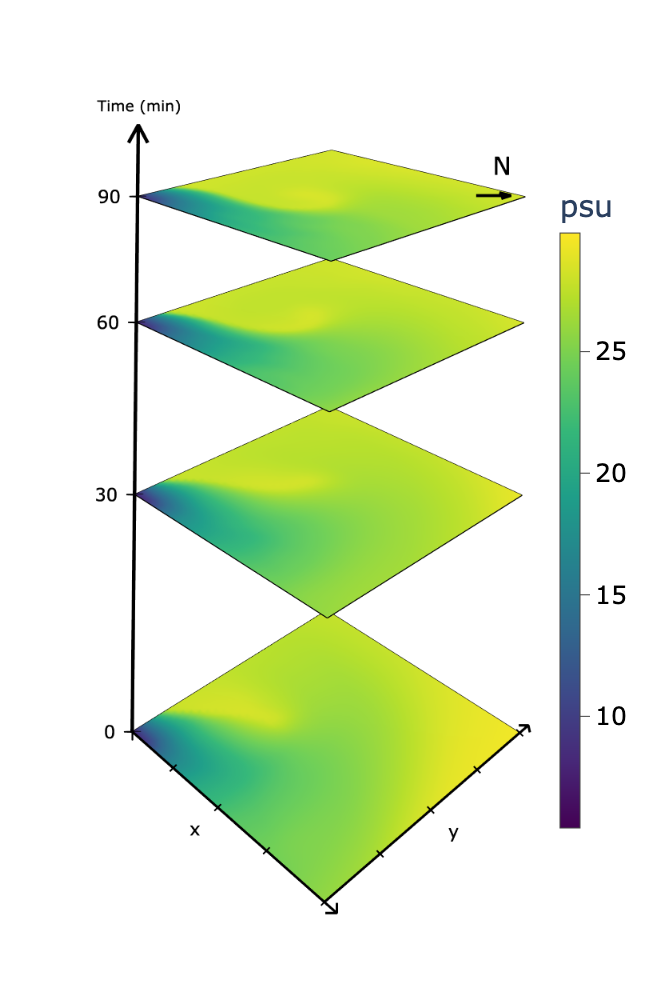
(c)

Figure 5: Visualization of the salinity data generated by the numerical model (SINMOD). The three panels show three time segments of 90 minutes on May 27, 2021. Salinity is measured in PSU (practical salinity units) i.e., g/kg.

The goal is to compare the proposed complex non-separable model to a separable model to evaluate how much is gained by a non-separable model. In this application, the true physical process (and the numerical model) clearly has non-separable phenomena such as diffusion and advection, which gives a good platform to evaluate the proposed approach. Previous works have in general employed purely spatial GRFs onboard the AUVs for real-time prediction, interpolation, and monitoring (Fossum et al.,, 2021; Ge et al.,, 2023; Berild et al.,, 2024). However, a strong disadvantage is that the ocean is dynamic, and assuming that the field is constant in time is not realistic for the general duration of an AUV mission, but it does speed up the onboard computations. Furthermore, many of these approaches have used adaptive sampling strategies to choose locations for the AUV to collect measurements, but since our main focus is prediction accuracy, we will generate random paths for the AUV to follow.

5.2 Estimating the surrogate models

The area of interest spans $1568\,\mathrm{m}\times 1408\,\mathrm{m}$, and we use a discretization of $M=50$ cells in $x$-direction and $N=45$ cells in $y$-direction, which gives a total of $K=M\cdot N=2250$ spatial locations. In addition, a buffer around the field is added to mitigate the effect of the boundaries of the field, and the total area is $M=60$ cells in $x$-direction and $N=55$ cells in $y$-direction. There is also added an advection tapering within this buffer to mitigate the effects of the boundaries even further. This area is large enough to capture the dynamics of the river outlet and the surrounding area, and with the number of timesteps would be unpractical to handle with classical spatio-temporal models. We use May 27, 2021, for estimating the model, termed the training data. This is 144 timesteps, where each time step is 10 min, and we split the dataset into $9$ non-overlapping time segments of $T=9$ timesteps (90 minutes) with one hour between each segment to avoid temporal correlation between them.

We collect the training data from each time segment as $\bm{y}_{1},\ldots,\bm{y}_{m},\ldots,\bm{y}_{9}$, where $\bm{y}_{m}=(y_{m,1,1},\ldots,y_{m,k,t},\ldots,y_{m,K,T})^{\top}$ is the salinity field of $m$th time segment. Since this data has a trend that varies through time and the time segments are assumed to be independent of each other, we remove this trend by subtracting the mean of each time segment from the data as $\tilde{\bm{y}}_{m}=\bm{y}_{m}-\bar{\bm{y}}_{m}$, where $\bar{\bm{y}}_{m}$ is the mean over the time segment for each location in space

$$\bar{\bm{y}}_{m}=\frac{1}{T}\sum_{t=1}^{T}\bm{y}_{m,t}.$$

Here, $\bm{y}_{m,t}=(y_{m,t,1},\ldots,y_{m,t,K})^{\top}$ is the spatial salinity field at time $t$ for the $m$th time segment. The models are then estimated on the resulting residuals of the detrended SINMOD data with observation model

$$\tilde{\bm{y}}_{m}=\mathbf{E}{\bm{w}}_{m}+\bm{\epsilon}_{m},\quad m=1,\ldots,9,$$

where ${\bm{w}}_{1},\ldots,{\bm{w}}_{9}|\bm{\theta}\overset{\text{iid}}{\sim}{\cal N}(\bm{0},\mathbf{Q}^{-1}(\bm{\theta}))$ with the model parameters $\bm{\theta}$ and $\bm{\epsilon}_{1},\ldots,\bm{\epsilon}_{9}|\sigma_{n}^{2}\overset{\text{iid}}{\sim}\mathcal{N}(\bm{0},\sigma_{n}^{2}\mathbf{I})$.

We consider the proposed flexible stochastic diffusion-advection-reaction model termed NStat-AD and the complex non-stationary separable model termed NStat-Sep described in Section 4.3. In terms of the initial values of the parameters, it is quite easy to make reasonable guesses for the advection parameters as they most likely will be similar to the currents which are generally pointed to the North (given by SINMOD output). The diffusion parameters are harder to suggest but are initially set perpendicular to the advection vector field.

Figure 6 shows the estimated marginal variance for NStat-AD, and visualizes the estimated correlation with the marked location in space and time, and all other locations. Here, we can observe that the model has captured some spatially varying dynamics in the SINMOD data. The correlation shows that there is an advection effect towards the north and a possible diffusion effect towards the east (or west). We also observe that the variance of the field is higher where the river outlet is located, which is reasonable as the river will introduce varying freshwater that is affected by the tides and the currents in the area.

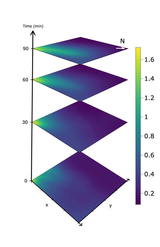
(a) Variance

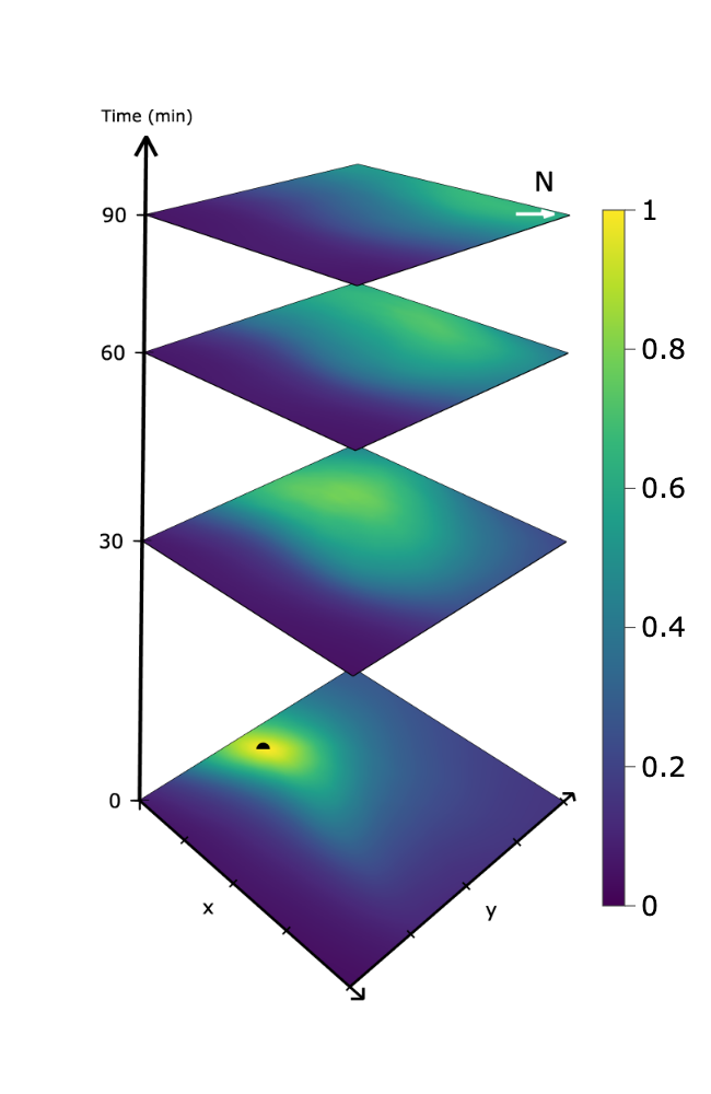
(b) Correlation

Figure 6: The marginal variance (a) and the correlation (b) of the NStat-AD model estimated on SINMOD data from the 27th of May 2021. The marked location is the location in space and time where the correlation is visualized.

5.3 Evaluating the surrogate models

The test dataset is comprised of simulation data from SINMOD spanning nine different days: May 28, May 29, May 4, May 10, May 11 in 2021, and June 21, June 22, September 8, and September 9 in 2022. The setup for the test data mirrors that of the training data and includes 72 time segments, each treated as independent from one another and from the training set. However, the test data is not detrended as the training data, as the emulator is expected to predict the salinity field directly from measurements. Therefore, the observation model for the test data is given by

$$\bm{y}_{m}=\bm{\mu}+\mathbf{E}{\bm{w}}_{m}+\bm{\epsilon}_{m},\quad m=1,\ldots,72,\quad\bm{\epsilon}\sim\mathcal{N}(\bm{0},\sigma_{n}^{2}\mathbf{I}),$$

where $\bm{\mu}=(\bm{\mu}_{\mathrm{S}},\ldots,\bm{\mu}_{\mathrm{S}})^{\top}$ stacked $T$ times with $\bm{\mu}_{\mathrm{S}}$ which is the spatially varying empirical mean of the training data across all time segments. In real-world applications, it might not be feasible to develop surrogate models that are specifically tailored for the exact dates and durations of upcoming missions. Therefore, testing the models with SINMOD data from different days in this simulated environment serves as an effective way to assess the models’ adaptability and predictive accuracy.

We assume that the AUV moves at a constant speed of $0.5\,\mathrm{m/s}$, with each mission lasting 90 minutes, matching the time segments of the model. The AUV’s trajectories are designed as random walks that minimize path intersections, favor straight-line movement, and remain within the designated area of interest. An example of such a path is depicted in Figure 7(a). In practical scenarios, AUVs would collect data at specific intervals; however, for this simulation, we assume data collection occurs whenever the AUV enters a new grid cell or a new time step begins. This data collection procedure is very similar to the result of data assimilation done with finite volume solution of the SPDE model (Berild et al.,, 2024). For this study, we generated 200 such random paths, and the specific paths employed are illustrated in Figure 7(b).

For each of the 72 time segments and 200 simulated paths, measurements are collected with a measurement error variance of $\sigma_{n}^{2}=0.01$. This measurement error is introduced to compensate for the deterministic and overly smooth outputs of the SINMOD model, simulating the noise typically found in real-world data. In total, this is 14400 different missions, and for each of them the estimated surrogate models are updated with the respective measurements to obtain the posterior distributions. The posterior mean serves as the spatial and temporal point prediction, with accuracy assessed via the RMSE on unobserved points for each mission. We then calculate both the mean and standard deviation of the RMSE across all paths for each dataset. To evaluate the predictive distribution further, the CRPS is computed for each mission. Similarly, the mean and standard deviation of the CRPS are calculated across the 200 paths for each of the 72 datasets.

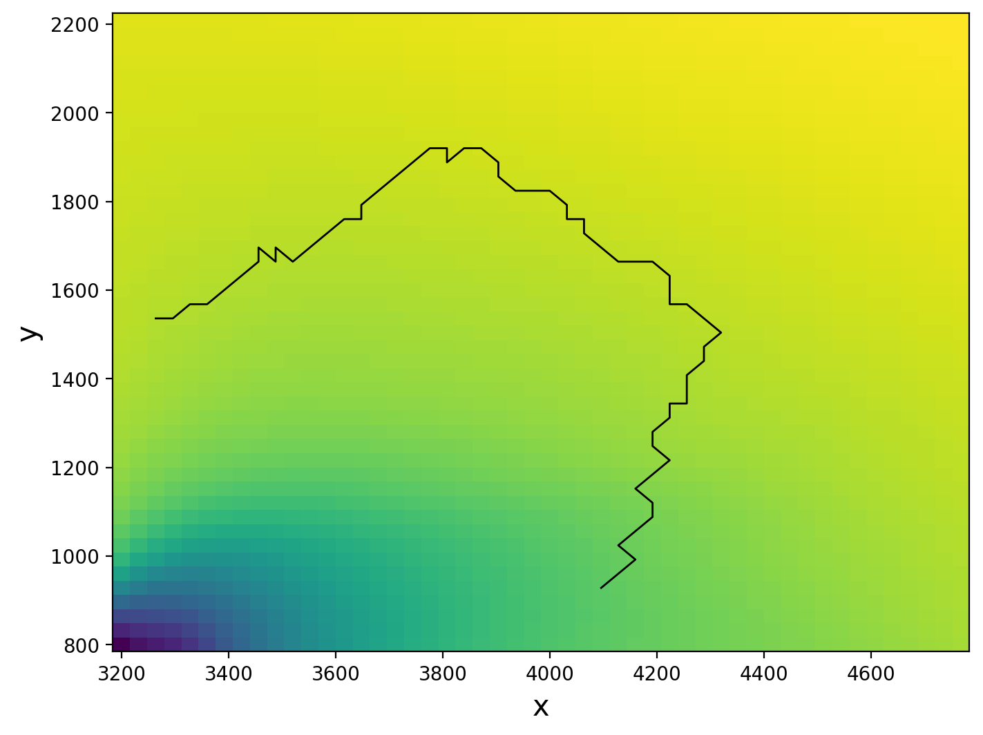
(a) One path

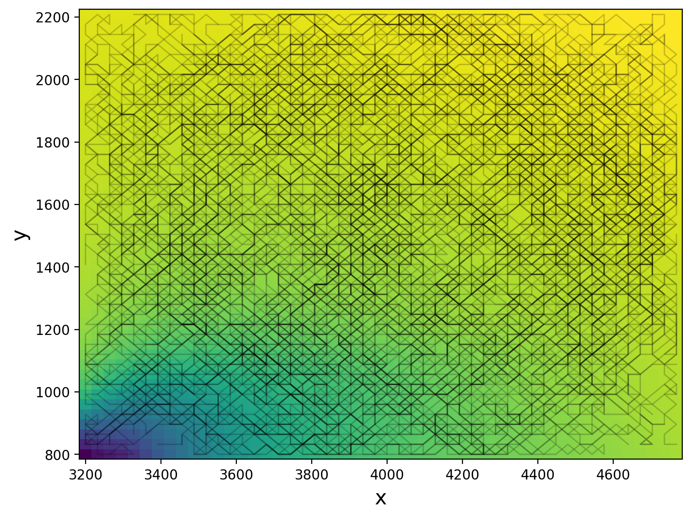
(b) All paths

Figure 7: Illustation of one randomly generate AUV path (a) and all 200 paths (b) used in the evaluation of the surrogate models.

5.4 Results

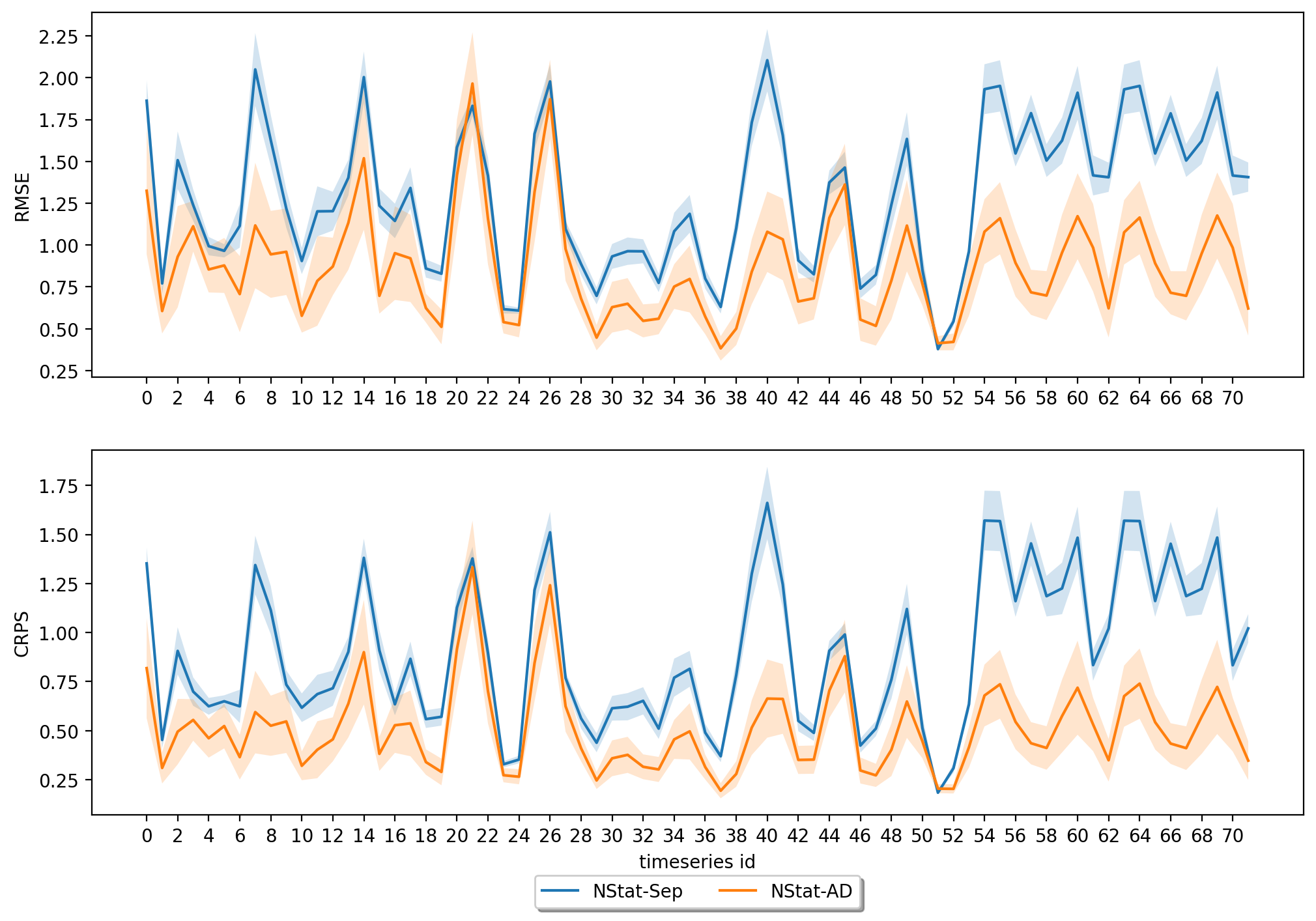
Figure 8: The RMSE (a) and the CRPS (b) for the 72 datasets used in the evaluation of the statistical emulators. The shaded regions are the standard deviations of the respective metrics across the 200 paths. The x-axis shows the different datasets and the y-axis shows the RMSE and the CRPS. The blue line represents the NStat-AD model, and the orange line represents the NStat-Sep model.

The comparative evaluation of the two surrogate models is depicted in Figure 8. The results indicate that the NStat-AD model generally outperforms the NStat-Sep model in terms of both RMSE and CRPS across most time segments, with a few exceptions where the NStat-Sep model performs marginally better. This divergence is likely due to instances where the conditions significantly deviate from those in the training data, causing the more complex NStat-AD model to yield less accurate predictions.

The error bands, representing the standard deviations of the RMSE and CRPS across the 200 paths, show greater variability for the NStat-AD model compared to the NStat-Sep model. This increased variation is anticipated given the higher accuracy of the NStat-AD model, making it more sensitive to less informative AUV paths. Despite this variability, the NStat-AD model consistently outperforms the NStat-Sep model overall, even when considering this variation.

6 Discussion

We are able to estimate spatially varying advection and diffusion by using bases of tensor product B-splines for the coefficients in the SPDE. The model with advection and diffusion performed better than a non-stationary separable spatio-temporal model, which struggled with advection and diffusion. In the simulation study, we even saw that the simplified non-separable model outperformed the more complex non-stationary separable model.

Stationary models are contained in the new model class by using one parameter per coefficient instead of basis functions. The estimated models are interpretable through an initial distribution, and the diffusion tensor and advection vector field. Further, in the advection-dominated simulation study, we do not observe the instability seen by Clarotto et al., (2023) for their FEM approximation. This suggests that FVM is a promising alternative to FEM for this problem.

In the simulation study, we found that while the complex models substantially outperformed the simpler ones for forecasting, they only showed a marginal improvement in reconstruction tasks. This suggests that correctly modeling the spatio-temporal dynamics is more important for forecasting than for interpolation. The predictive performance of the complex model closely mirrored that of the true model, affirming our ability to accurately estimate its parameters even when a sub-area was missing.

The potential applications for this approach are vast, as advection and diffusion are natural first approximations of spatio-temporal dynamics. However, one may need more complex mechanisms to capture, for example, long-distance coupling. A key challenge for practical application lies in acquiring sufficient data to accurately estimate the proposed model. In cases where data is more sparse, it will be necessary to incorporate penalties or priors that limit the spatial variation of the coefficients in the SPDE. Determining the appropriate strength of the penalties can be challenging for non-stationary models (Fuglstad et al., 2015b, ). Before applying the proposed model to such settings, one would need to investigate appropriate penalties and priors.

An intriguing extension of our proposed approach involves the local refinement of tensor product B-splines (Patrizi et al.,, 2020). This refinement adjusts the placement of knots within the B-splines depending on where increased flexibility is required or where less is beneficial. Another potential enhancement is the adoption of triangular instead of rectangular grid cells. This modification would offer enhanced flexibility in the spatial domain, allowing for more accurate representations of complex geographical features like coastlines, islands, and fjords. While these extensions would necessitate additional implementation efforts, they present valuable opportunities for further research and development in future projects.

Optimizing our model presents several challenges and opportunities for improvement. One notable limitation is that the vector field describing the anisotropic diffusion exhibits two equivalent optima, complicating optimization efforts, particularly since this vector field varies spatially. Exploring alternative parameterizations of the vector field that circumvent this issue could be beneficial. In our efforts to optimize the model parameters, we have utilized the ADAM optimizer (Kingma and Ba,, 2017), chosen for its effectiveness in handling vanishing gradients—a common issue in machine learning scenarios where certain parameter gradients are extremely small. Despite its advantages, ADAM is not without flaws, and there may be potential for better performance with other optimizers. We have tested additional optimizers, including Rmsprop, Adagrad, and Adadelta (Ruder,, 2017), but none outperformed ADAM in our studies. We also experimented with AdaHessian (Yao et al.,, 2021), which scales gradients using the diagonal of the Hessian matrix. However, this approach did not enhance the optimization process, likely because the parameters are too interdependent to benefit from scaling by only the diagonal elements. Calculating the full Hessian matrix, while potentially more effective, is prohibitively expensive in computational terms for this model. Exploring these optimization challenges further could yield significant advancements in the performance and applicability of our approach.

Author Contributions

Martin Outzen Berild performed writing - original Draft, development of the software, and the methodology, and Geir-Arne Fuglstad contributed with writing - original draft, conceptualization, and supervision.

Funding

This work is funded by the Norwegian Research Council through the MASCOT project 305445.

Appendix A. Discretizing the advection-diffusion SPDE

A.1 Problem formulation

In this part, we will consider the stochastic advection-diffusion-reaction equation,

$$\frac{\partial}{\partial t}u(\bm{s},t)+(\kappa^{2}(\bm{s})-\nabla\cdot\mathbf{H}(\bm{s})\nabla)u(\bm{s},t)+\nabla\cdot(\bm{\omega}(\bm{s})u(\bm{s},t))=\tau\frac{\partial}{\partial t}B(\bm{s},t).$$ (S1)

for $\bm{s}\in\mathcal{D}\subset\mathbb{R}^{2}$, where $\mathcal{D}$ is the spatial domain, and $t\in\mathcal{T}$, where $\mathcal{T}$ is the temporal domain. Here, $\kappa(\cdot)$ is a positive function, $\mathbf{H}(\cdot)$ is a spatially varying $2\times 2$ positive definite matrix, $\bm{\omega}(\cdot)$ is a vector field, $\tau>0$ is a constant, and $B(\cdot,\cdot)$ is the Q-Wiener process defined in Section 2.2 through $\text{WM}(\kappa_{\mathrm{F}}(\cdot),\mathbf{H}_{\mathrm{F}}(\cdot))$. Compared to Equation (6), we skip the subscript “E” to ease notation in the derivations that follow. We consider no flow boundary conditions,

$$\left(\mathbf{H}(\bm{s})\nabla u(\bm{s},t)+\bm{\omega}(\bm{s})u(\bm{s},t)\right)\cdot{\bm{n}}(\bm{s})=0,\quad\bm{s}\in\partial\mathcal{D},\quad t\in\mathcal{T},$$

where ${\bm{n}}(\cdot)$ is the outwards normal vector at the boundary.

We assume:

• the spatial domain is rectangular $\mathcal{D}=[A_{1},A_{2}]\times[B_{1},B_{2}]$, where $A_{1}<A_{2}$ and $B_{1}<B_{2}$;

• the temporal domain is $\mathcal{T}=(0,T_{\mathrm{t}}]$, where $T_{\mathrm{t}}>0$ is the terminal time.

• the initial condition is $u(\cdot,0)\sim\text{WM}(\kappa_{\mathrm{I}}(\cdot),\mathbf{H}_{\mathrm{I}}(\cdot))$

A.2 Temporal discretization

We use a regular temporal grid where $0=t_{0}^{\mathrm{G}}<t_{1}^{\mathrm{G}}<\cdots<t_{T-1}^{\mathrm{G}}=T_{\mathrm{t}}$, and the time step length is $\Delta t$. Let $u^{n}(\cdot)=u(\cdot,t_{n}^{\mathrm{G}})$ and $B^{n}(\cdot)=B(\cdot,t_{n}^{\mathrm{G}})$ for $n=0,\ldots,T-1$. Then using backward Euler on Equation (S1) gives

$$u^{n+1}(\cdot) =u^{n}(\cdot)$$ (S2)

$$\phantom{=}+\Delta t\left\{-\left[\kappa(\cdot)^{2}-\nabla\cdot\mathbf{H}(\cdot)\nabla\right]u^{n+1}(\cdot)+\nabla\cdot(\bm{\omega}(\cdot)u^{n+1}(\cdot))\right\}+$$

$$\phantom{=}+\tau(B^{n+1}(\cdot)-B^{n}(\cdot)),$$

for $n=0,1,\ldots,T-2$. From the definition of $B(\cdot,\cdot)$, we have that

$$(B^{1}(\cdot)-B^{0}(\cdot))/\sqrt{\Delta t},\ldots,(B^{T-1}(\cdot)-B^{T-1}(\cdot))/\sqrt{\Delta t}\overset{\text{iid}}{\sim}\text{WM}(\kappa_{\mathrm{F}}(\cdot),\mathbf{H}_{\mathrm{F}}(\cdot)).$$

The GRFs $u^{0}(\cdot),\ldots,u^{T-1}(\cdot)$ gives an approximation that is discrete in time, but continuous in space.

A.3 Spatial discretization

Divide the rectangle $\mathcal{D}=[A_{1},A_{2}]\times[B_{1},B_{2}]$ into a regular grid of $M$ cells in the $x$-direction and $N$ cells in the $y$-direction. The grid cells are indexed by $i=0,\ldots,M-1$ and $j=0,\ldots,N-1$ in the $x$- and $y$-direction, respectively. The grid cell centers are denoted by $\bm{s}_{i,j}=(x_{i},y_{j})$, and the side length of the grid cells are denoted by $h_{x}=(A_{2}-A_{1})/M$ and $h_{y}=(B_{2}-B_{1})/N$. A visualization of the discretized spatial domain is shown in Figure S1.

Figure S1: Visualization of the discretizated spatial domain.

The volume/area of each grid cell is denoted by $V_{i,j}=h_{x}h_{y}$. We denote the grid cell by $E_{i,j}\subset\mathcal{D}$ and the boundary of the grid cell by $\partial E_{i,j}$. The boundary of each grid cell consists of four faces (or edges) denoted by $A_{i,j}^{\text{Left}}$, $A_{i,j}^{\text{Right}}$, $A_{i,j}^{\text{Top}}$, and $A_{i,j}^{\text{Bottom}}$. We denote the centers of the respective faces as $\bm{s}_{i+1/2,j}$, $\bm{s}_{i-1/2,j}$, $\bm{s}_{i,j+1/2}$, and $\bm{s}_{i,j-1/2}$. See Figure S2 for a visualization.

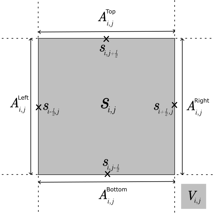
Figure S2: A visualization of a grid cell. The cell volume $V_{i,j}$ is shown in gray.

We apply FVM and integrate the temporally discretized Equation (S2) over a cell,

$$\int_{E_{i,j}}u^{n+1}(\bm{s})\mathrm{d}\bm{s}=\int_{E_{i,j}}u^{n}(\bm{s})\mathrm{d}\bm{s}$$

$$-\Delta t\left\{\int_{E_{i,j}}\kappa^{2}(\bm{s})u^{n+1}(\bm{s})\mathrm{d}\bm{s}-\int_{E_{i,j}}\nabla\cdot\mathbf{H}(\bm{s})\nabla u^{n+1}(\bm{s})\mathrm{d}\bm{s}+\int_{E_{i,j}}\nabla\cdot\bm{\omega}(\bm{s})u^{n+1}(\bm{s})\mathrm{d}\bm{s}\right\}$$

$$+\int_{E_{i,j}}\tau(B^{n+1}(\bm{s})-B^{n}(\bm{s}))\mathrm{d}\bm{s},$$

The integrals on the first line and the first term on the second line is approximated by assuming that the integrands are constant in the grid cells. I.e.,

$$\int_{E_{i,j}}u^{n+1}(\bm{s})\mathrm{d}\bm{s}\approx V_{i,j}u_{i,j}^{n+1},\quad\int_{E_{i,j}}u^{n}(\bm{s})\mathrm{d}\bm{s}\approx V_{i,j}u_{i,j}^{n}$$

$$\text{and}\quad\int_{E_{i,j}}\kappa^{2}(\bm{s})u^{n+1}(\bm{s})\mathrm{d}\bm{s}\approx V_{i,j}\kappa^{2}_{i,j}u_{i,j}^{n+1},$$

where $\kappa^{2}_{i,j}=\kappa(\bm{s}_{i,j})^{2}$ and $u_{i,j}^{n+1}=u^{n+1}(\bm{s}_{i,j})$. Similarily for the last term

$$\int_{E_{i,j}}\tau(B^{n+1}(\bm{s})-B^{n}(\bm{s}))\mathrm{d}\bm{s}\approx V_{i,j}\tau(B^{n+1}_{i,j}-B^{n}_{i,j})\approx V_{i,j}\tau\sqrt{\Delta t}\phi_{i,j}^{n},$$

where $B^{n}_{i,j}=B^{n}(\bm{s}_{i,j})$, and $\phi_{1,1}^{n},\ldots,\phi_{M,N}^{n}$ arises from FVM applied to the purely spatial problem $\text{WM}(\kappa_{\mathrm{F}}(\cdot),\mathbf{H}_{\mathrm{F}}(\cdot))$. We refer to Fuglstad et al., 2015a ; Fuglstad et al., 2015b for details on discretizing a spatial SPDE with FVM. However, the end result is that $\bm{\phi}^{n}=(\phi_{1,1}^{n},\ldots,\phi_{M,N}^{n})\sim\mathcal{N}(\bm{0},\mathbf{Q}_{\mathrm{F}}^{-1})$ for a sparse matrix $\mathbf{Q}_{\mathrm{F}}$ and $\bm{\phi}^{0},\ldots,\bm{\phi}^{T-2}$ are independent.

To handle the integrals of the advection and diffusion terms, we use the divergence theorem

$$\int_{E_{i,j}}\nabla\cdot\mathbf{F}(\bm{s})\enspace\mathrm{d}\bm{s}=\oint_{\partial E_{i,j}}\mathbf{F}(\bm{s})\cdot\bm{n}(\bm{s})\enspace\mathrm{d}A,$$

where $\mathbf{F}(\cdot)$ is a vector field, $\bm{n}(\cdot)$ is outward-facing normal vector to the respective faces, $\mathrm{d}A$ is the line element, and the line integral follows the positive orientation. This gives

$$\int_{E_{i,j}}\nabla\cdot\mathbf{H}(\bm{s})\nabla u^{n+1}(\bm{s})\mathrm{d}\bm{s} =\oint_{\partial E_{i,j}}\nabla u^{n+1}(\bm{s})\cdot(\mathbf{H}(\bm{s})\bm{n}(\bm{s}))\mathrm{d}A,$$

$$\int_{E_{i,j}}\nabla\cdot\bm{\omega}(\bm{s})u^{n+1}(\bm{s})\mathrm{d}\bm{s} =\oint_{\partial E_{i,j}}u^{n+1}(\bm{s})(\bm{\omega}(\bm{s})\cdot\bm{n}(\bm{s}))\mathrm{d}A.$$

Thus using the approximations and the divergence theorem,

$$V_{i,j}u_{i,j}^{n+1} =V_{i,j}u_{i,j}^{n}-\Delta tV_{i,j}\kappa^{2}_{i,j}u_{i,j}^{n+1}$$ (S3)

$$\phantom{=}-\Delta t\oint_{\partial E_{i,j}}\left[\nabla u^{n+1}(\bm{s})\cdot(\mathbf{H}(\bm{s}){\bm{n}}(\bm{s}))+u^{n+1}(\bm{s})(\bm{\omega}(\bm{s})\cdot{\bm{n}}(\bm{s})\right]\mathrm{d}A$$

$$\phantom{=}+V_{i,j}\tau\sqrt{\Delta t}\phi_{i,j}^{n+1}.$$

The second line is subtracting the net flow leaving the grid cell. For approximating the flow arising from diffusion we refer to Fuglstad et al., 2015a , and we detail the approximation of the flow arising from advection in the next subsection. Note that the zero flow boundary condition means that the line integral on the second line is 0 on faces that belong to the boundary, which is desired as there should be zero flow out of the boundary.

A.4 Approximating flow arising from advection

We consider a generic time step and drop superscripts to denote dependence on the time step, and decompose and approximate the net flow out of the domain from advection term in Equation (S3) as

$$\oint_{\partial E_{i,j}}u(\bm{s})(\bm{\omega}(\bm{s})\cdot{\bm{n}}(\bm{s}))\mathrm{d}A\approx\hat{W}_{i,j}^{\text{Right}}+\hat{W}_{i,j}^{\text{Left}}+\hat{W}_{i,j}^{\text{Top}}+\hat{W}_{i,j}^{\text{Bottom}},$$

where the integral is split into integrals over each face that are approximated as

$$\int_{A_{i,j}^{\text{Dir}}}u(\bm{s})\left(\bm{\omega}(\bm{s})\cdot{\bm{n}}(\bm{s})\right)\mathrm{d}A\approx u(\bm{s}_{i,j})^{\text{Dir}}\left(\bm{\omega}(\bm{s}_{i,j}^{\text{Dir}})\cdot{\bm{n}}(\bm{s}_{i,j}^{\text{Dir}})\right)\int_{A_{i,j}^{\text{Dir}}}\mathrm{d}A$$

$$= u(\bm{s}_{i,j}^{\text{Dir}})\left(\bm{\omega}(\bm{s}_{i,j}^{\text{Dir}})\cdot{\bm{n}}(\bm{s}_{i,j}^{\text{Dir}})\right)|A_{i,j}^{\text{Dir}}|$$

$$= \tilde{W}_{i,j}^{\text{Dir}}.$$

Here, $|A_{i,j}^{\text{Dir}}|$ is the length of the face $A_{i,j}^{\text{Dir}}$, and $\bm{s}_{i,j}^{\text{Dir}}$ is the center of the face $A_{i,j}^{\text{Dir}}$, i.e. if the right face is considered $|A_{i,j}^{\text{Right}}|=h_{y}$ and $\bm{s}_{i,j}^{\text{Right}}=\bm{s}_{i+1/2,j}$.

We use an upwind scheme, where we take the direction of the flow into account. When considering the flow over a given face, we only consider the upwind cell according to the advection vector field at the centre of the face. E.g., if we are considering the right face of a grid cell and the flow goes to the left, we use the value of the field in the grid cell to the right. This is known to help with numerical stability and is a common scheme in the finite volume method.

Let $\omega^{x}_{i\pm 1/2,j}$ denote the $x$-component of $\bm{\omega}(\bm{s}_{i\pm 1/2,j})$ and $\omega^{y}_{i,j\pm 1/2}$ denote the $y$-component of $\bm{\omega}(\bm{s}_{i,j\pm 1/2})$. First, we consider the right face, and the upwind scheme gives

$$\hat{W}_{i,j}^{\text{Right}}=h_{y}\left[\frac{|\omega_{i+1/2,j}^{x}|+\omega_{i+1/2,j}^{x}}{2}u_{i,j}-\frac{|\omega_{i+1/2,j}^{x}|-\omega_{i+1/2,j}^{x}}{2}u_{i+1,j}\right].$$

Similarly, we have for the left face

$$\hat{W}_{i,j}^{\text{Left}}=h_{y}\left[\frac{|\omega_{i-1/2,j}^{x}|-\omega_{i-1/2,j}^{x}}{2}u_{i,j}-\frac{|\omega_{i-1/2,j}^{x}|+\omega_{i-1/2,j}^{x}}{2}u_{i-1,j}\right],$$

and for the top and bottom faces,

$$\hat{W}_{i,j}^{\text{Top}}=h_{x}\left[\frac{|\omega_{i,j+1/2}^{y}|+\omega_{i,j+1/2}^{y}}{2}u_{i,j}-\frac{|\omega_{i,j+1/2}^{y}|-\omega_{i,j+1/2}^{y}}{2}u_{i,j+1}\right],$$

$$\hat{W}_{i,j}^{\text{Bottom}}=h_{x}\left[\frac{|\omega_{i,j-1/2}^{y}|-\omega_{i,j-1/2}^{y}}{2}u_{i,j}-\frac{|\omega_{i,j-1/2}^{y}|+\omega_{i,j-1/2}^{y}}{2}u_{i,j-1}\right].$$

We vectorize the above expressions and define the vector of all spatial locations for timestep $n+$ as

$${\bm{u}}^{n}=(u_{0,0}^{n},u_{1,0}^{n},\ldots,u_{M-1,0}^{n},u_{0,1}^{n},u_{1,1}^{n},\ldots,u_{M-1,N-1}^{n})^{\top},$$

for $n=0,\ldots,T-1$. We introduce the advection matrix $\mathbf{A}_{\bm{\omega}}$ such that $\mathbf{A}_{\bm{\omega}}{\bm{u}}^{n+1}$ gives the advection term in Equation (S3) using the above approximations. Thus $\mathbf{A}_{\bm{\omega}}$ is a $MN\times MN$ matrix, where the local solution of the advection term for location $(i,j)$ is collected in the $(jM+i)$th row of the matrix. In the following equations, we show the non-zero elemests. For the diagonal elements we have

$$\left(\mathbf{A}_{\bm{\omega}}\right)_{jM+i,jM+i}= \frac{h_{y}}{2}\left[|\omega_{i+1/2,j}^{x}|+\omega_{i+1/2,j}^{x}+|\omega_{i-1/2,j}^{x}|-\omega_{i-1/2,j}^{x}\right]+$$

$$+\frac{h_{x}}{2}\left[|\omega_{i,j+1/2}^{y}|+\omega_{i,j+1/2}^{y}+|\omega_{i,j-1/2}^{y}|-\omega_{i,j-1/2}^{y}\right].$$

Let $i_{p}=i+1$, $i_{n}=i-1$, $j_{p}=j+1$, and $j_{n}=j-1$, then the $(jM+i_{p})$th, $(jM+i_{n})$th, $(j_{p}M+i)$th, and $(j_{n}M+i)$th elements of the $(jM+i)$th row are

$$\left(\mathbf{A}_{\bm{\omega}}\right)_{jM+i,jM+i_{p}}=-\frac{h_{y}}{2}\left(|\omega_{i+1/2,j}^{x}|-\omega_{i+1/2,j}^{x}\right),$$

$$\left(\mathbf{A}_{\bm{\omega}}\right)_{jM+i,jM+i_{n}}=-\frac{h_{y}}{2}\left(|\omega_{i-1/2,j}^{x}|+\omega_{i-1/2,j}^{x}\right),$$

$$\left(\mathbf{A}_{\bm{\omega}}\right)_{jM+i,j_{p}M+i}=-\frac{h_{x}}{2}\left(|\omega_{i,j+1/2}^{y}|-\omega_{i,j+1/2}^{y}\right),$$

$$\left(\mathbf{A}_{\bm{\omega}}\right)_{jM+i,j_{n}M+i}=-\frac{h_{x}}{2}\left(|\omega_{i,j-1/2}^{y}|+\omega_{i,j-1/2}^{y}\right).$$

A.5 The fully descritized SPDE and the precision matrix

Combining all previous steps, the fully discretized problem can be written in vector form as

$$\left(\mathbf{D}_{\mathrm{V}}+\Delta t(\mathbf{D}_{\mathrm{V}}\mathbf{D}_{\kappa^{2}}-\mathbf{A}_{\mathbf{H}}+\mathbf{A}_{\bm{\omega}})\right){\bm{u}}^{n+1}=\mathbf{D}_{\mathrm{V}}{\bm{u}}^{n}+\tau\sqrt{\Delta t}\mathbf{D}_{\mathrm{V}}\bm{\phi}^{n},$$

where $\bm{\phi}^{n}=\mathbf{L}_{\mathrm{F}}^{-{\top}}\bm{\epsilon}^{n}$ is the spatially smoothed innovations arising from $\bm{\epsilon}^{0},\ldots,\bm{\epsilon}^{n+1}\overset{\text{iid}}{\sim}{\cal N}(0,\mathbf{I})$, where $\mathbf{L}_{\mathrm{F}}$ is the Cholesky factor so that $\mathbf{Q}_{\mathrm{F}}=\mathbf{L}_{\mathrm{F}}\mathbf{L}_{\mathrm{F}}^{\top}$. We simply the notation by introducing

$$\mathbf{A}= \mathbf{D}_{\mathrm{V}}+\Delta t\left(\mathbf{D}_{\mathrm{V}}\mathbf{D}_{\kappa^{2}}-\mathbf{A}_{\mathbf{H}}+\mathbf{A}_{\bm{\omega}}\right),$$

$$\mathbf{G}= \mathbf{A}^{-1}\mathbf{D}_{\mathrm{V}},$$

$$\mathbf{E}= \tau\sqrt{\Delta t}\mathbf{A}^{-1}\mathbf{D}_{\mathrm{V}}\mathbf{L}_{\mathrm{F}}^{-{\top}}.$$

Then the forward equations in time is

$${\bm{u}}^{n+1}=\mathbf{G}{\bm{u}}^{n}+\mathbf{E}\bm{\epsilon}^{n},\quad n=0,\ldots,T-2,$$

where ${\bm{u}}^{0}\sim\mathcal{N}(\bm{0},\mathbf{Q}_{0})$ arising from approximating $\text{WM}(\kappa_{\mathrm{I}}(\cdot),\mathbf{H}_{\mathrm{I}}(\cdot))$. However, note that computationally one would not compute the dense matrices $\mathbf{G}$ and $\mathbf{E}$ when using this equation for simulation.

Let us now collect all these timesteps into the vectors

$${\bm{u}}=\begin{bmatrix}{\bm{u}}^{0}\\ {\bm{u}}^{1}\\ \vdots\\ {\bm{u}}^{T-1}\end{bmatrix},\quad\text{and}\quad\bm{\epsilon}=\begin{bmatrix}\bm{\epsilon}^{0}\\ \vdots\\ \bm{\epsilon}^{T-2}\end{bmatrix}.$$

We then have

$${\bm{u}}=\mathbf{R}\begin{bmatrix}{\bm{u}}^{0}\\ \bm{\epsilon}\end{bmatrix},$$ (S4)

where $\mathbf{R}$ is a block matrix constructed from the matrices $\mathbf{G}$ and $\mathbf{E}$ as

$$\mathbf{R}=\begin{bmatrix}\mathbf{I}&0&0&0&\dots&0&0\\ \mathbf{G}&\mathbf{E}&0&0&\dots&0&0\\ \mathbf{G}^{2}&\mathbf{G}\mathbf{E}&\mathbf{E}&0&\dots&0&0\\ \mathbf{G}^{3}&\mathbf{G}^{2}\mathbf{E}&\mathbf{G}\mathbf{E}&\mathbf{E}&\dots&0&0\\ \vdots&\vdots&\vdots&\vdots&\ddots&\vdots&\vdots\\ \mathbf{G}^{T-1}&\mathbf{G}^{T-2}\mathbf{E}&\mathbf{G}^{T-3}\mathbf{E}&\mathbf{G}^{T-4}\mathbf{E}&\dots&\mathbf{G}\mathbf{E}&\mathbf{E}\end{bmatrix}.$$ (S5)

We have

$$\pi\left(\begin{bmatrix}{\bm{u}}^{0}\\ \bm{\epsilon}\end{bmatrix}\right)\propto\exp\left(-\frac{1}{2}\begin{bmatrix}({\bm{u}}^{0})^{\mathrm{T}}&\bm{\epsilon}^{\mathrm{T}}\end{bmatrix}\begin{bmatrix}\mathbf{Q}_{0}&0&\dots&0\\ 0&\mathbf{I}&\dots&0\\ \vdots&\vdots&\ddots&\vdots\\ 0&0&\dots&\mathbf{I}\\ \end{bmatrix}\begin{bmatrix}{\bm{u}}^{0}\\ \bm{\epsilon}\end{bmatrix}\right).$$

Equation (S4) is a linear transformation and we can write the distribution of ${\bm{u}}$ as

$$\pi({\bm{u}})\propto \exp\left(-\frac{1}{2}{\bm{u}}^{\top}\mathbf{Q}{\bm{u}}\right)$$

$$= \exp\left(-\frac{1}{2}{\bm{u}}^{\top}\mathbf{R}^{-{\top}}\begin{bmatrix}\mathbf{Q}_{0}&0&\dots&0\\ 0&\mathbf{I}&\dots&0\\ \vdots&\vdots&\ddots&\vdots\\ 0&0&\dots&\mathbf{I}\\ \end{bmatrix}\mathbf{R}^{-1}{\bm{u}}\right).$$

Because of the block structure of $\mathbf{R}$, we can find its inverse as

$$\mathbf{R}^{-1}=\begin{bmatrix}\mathbf{I}&0&0&0&\dots&0&0\\ -\mathbf{E}^{-1}\mathbf{G}&\mathbf{E}^{-1}&0&0&\dots&0&0\\ 0&-\mathbf{E}^{-1}\mathbf{G}&\mathbf{E}^{-1}&0&\dots&0&0\\ 0&0&-\mathbf{E}^{-1}\mathbf{G}&\mathbf{E}^{-1}&\dots&0&0\\ \vdots&\vdots&\vdots&\vdots&\ddots&\mathbf{E}^{-1}&\vdots\\ 0&0&0&0&\dots&-\mathbf{E}^{-1}\mathbf{G}&\mathbf{E}^{-1}\end{bmatrix},$$

where the inverse of $\mathbf{E}$ and the relationship $\mathbf{F}=\mathbf{E}\mathbf{E}^{\top}$ is given by

$$\mathbf{E}^{-1}= \frac{1}{\tau\sqrt{\Delta t}}\mathbf{L}_{\mathrm{F}}^{\mathrm{T}}\mathbf{D}_{V}^{-1}\mathbf{A}$$

$$\mathbf{F}^{-1}= \mathbf{E}^{-{\top}}\mathbf{E}^{-1}=\frac{1}{\tau^{2}\Delta t}\mathbf{A}^{\top}\mathbf{D}_{V}^{-1}\mathbf{Q}_{S}\mathbf{D}_{V}^{-1}\mathbf{A}.$$

Finally, we can express the global precision matrix as

$$\mathbf{Q}=\begin{bmatrix}\mathbf{Q}_{0}+\mathbf{G}^{\top}\mathbf{F}^{-1}\mathbf{G}&-\mathbf{G}^{\top}\mathbf{F}^{-1}&0&\dots&0\\ -\mathbf{F}^{-1}\mathbf{G}&\mathbf{F}^{-1}+\mathbf{G}^{\top}\mathbf{F}^{-1}\mathbf{G}&-\mathbf{G}^{\top}\mathbf{F}^{-1}&\ddots&0\\ \vdots&\ddots&\ddots&\ddots&\vdots\\ \vdots&\ddots&-\mathbf{F}^{-1}\mathbf{G}&\mathbf{F}^{-1}+\mathbf{G}^{\top}\mathbf{F}^{-1}\mathbf{G}&-\mathbf{G}^{\top}\mathbf{F}^{-1}\\ 0&\dots&0&-\mathbf{F}^{-1}\mathbf{G}&\mathbf{F}^{-1}\end{bmatrix}.$$

Appendix B. Code implementations

The models described in this work are implemented in the Python package currently named spdepy. The package is available at https://github.com/berild/spdepy and is under development. Currently, the package is not available on PyPI, but can be installed using poetry.

The package is built from scratch using mostly NumPy and Cython for C++ interaction. The construction of the precision matrix components is done in C++ in order to speed up the computations. The models are only available for 2D spatial fields with a time component, but an extension to 3D and time is possible.

Available models in the package are the advection-diffusion SPDE, the separable space-time model, and the Whittle-Matérn SPDE. The user is free to specify if the parameters are spatially varying or not, and many different combinations are allowed. For example, non-stationary anisotropic spatial fields or simply stationary isotropic fields, and spatially varying advection and diffusion with a simple stationary isotropic initial field or simple constant advection and spatially varying diffusion with a complex non-stationary anisotropic initial field. It is also possible to set the advection field as a covariate.

The user can choose which optimization algorithm to use; currently, the package supports gradient descent, Adadelta, Adagrad, Rmsprop, and Adam. All of which are stochastic as we use the Hutchinson estimator in the gradient calculations. Also implemented is the AdaHessian optimizer, but is unavailable in the current version.

Lastly, also included in the package is the ocean dataset generated from the numerical model SINMOD. It is split into three datasets, one for training, one for validation, and one for testing. The testing dataset consists of real measurements collected with an AUV that is not used in this work.

References

- Banerjee et al., (2003) Banerjee, S., Carlin, B. P., and Gelfand, A. E. (2003). Hierarchical Modeling and Analysis for Spatial Data. CRC Press.
- Banerjee et al., (2008) Banerjee, S., Gelfand, A. E., Finley, A. O., and Sang, H. (2008). Gaussian Predictive Process Models for Large Spatial Data Sets. Journal of the Royal Statistical Society. Series B (Statistical Methodology), 70(4):825–848.
- Berild and Fuglstad, (2023) Berild, M. O. and Fuglstad, G.-A. (2023). Spatially varying anisotropy for gaussian random fields in three-dimensional space. Spatial Statistics, 55:100750.
- Berild et al., (2024) Berild, M. O., Ge, Y., Eidsvik, J., Fuglstad, G.-A., and Ellingsen, I. (2024). Efficient 3D real-time adaptive AUV sampling of a river plume front. Frontiers in Marine Science, 10.
- Bolin and Kirchner, (2020) Bolin, D. and Kirchner, K. (2020). The Rational SPDE Approach for Gaussian Random Fields With General Smoothness. Journal of Computational and Graphical Statistics, 29(2):274–285.
- Cameletti et al., (2013) Cameletti, M., Lindgren, F., Simpson, D., and Rue, H. (2013). Spatio-temporal modeling of particulate matter concentration through the SPDE approach. AStA Advances in Statistical Analysis, 97(2):109–131.
- Carrizo Vergara et al., (2022) Carrizo Vergara, R., Allard, D., and Desassis, N. (2022). A general framework for SPDE-based stationary random fields. Bernoulli, 28.
- Clarotto et al., (2023) Clarotto, L., Allard, D., Romary, T., and Desassis, N. (2023). The SPDE approach for spatio-temporal datasets with advection and diffusion. arXiv:2208.14015 [math, stat].
- Cressie and Johannesson, (2008) Cressie, N. and Johannesson, G. (2008). Fixed rank kriging for very large spatial data sets. Journal of the Royal Statistical Society: Series B (Statistical Methodology), 70(1):209–226.
- Cressie and Wikle, (2011) Cressie, N. and Wikle, C. K. (2011). Statistics for spatio-temporal data. John Wiley & Sons.
- Da Prato and Zabczyk, (2014) Da Prato, G. and Zabczyk, J. (2014). Stochastic equations in infinite dimensions. Cambridge university press.
- Eidsvik et al., (2014) Eidsvik, J., Shaby, B. A., Reich, B. J., Wheeler, M., and Niemi, J. (2014). Estimation and Prediction in Spatial Models With Block Composite Likelihoods. Journal of Computational and Graphical Statistics, 23(2):295–315.
- Foss et al., (2022) Foss, K. H., Berget, G. E., and Eidsvik, J. (2022). Using an autonomous underwater vehicle with onboard stochastic advection-diffusion models to map excursion sets of environmental variables. Environmetrics, 33(1):e2702.
- Fossum et al., (2021) Fossum, T. O., Travelletti, C., Eidsvik, J., Ginsbourger, D., and Rajan, K. (2021). Learning excursion sets of vector-valued Gaussian random fields for autonomous ocean sampling. The Annals of Applied Statistics, 15(2):597 – 618.
- Fuglstad and Castruccio, (2020) Fuglstad, G.-A. and Castruccio, S. (2020). Compression of climate simulations with a nonstationary global spatiotemporal spde model. The Annals of Applied Statistics, 14(2):542–559.
- (16) Fuglstad, G.-A., Lindgren, F., Simpson, D., and Rue, H. (2015a). Exploring a new class of non-stationary spatial gaussian random fields with varying local anisotropy. Statistica Sinica, pages 115–133.
- (17) Fuglstad, G.-A., Simpson, D., Lindgren, F., and Rue, H. (2015b). Does non-stationary spatial data always require non-stationary random fields? Spatial Statistics, 14:505–531.
- Ge et al., (2023) Ge, Y., Eidsvik, J., and Mo-Bjørkelund, T. (2023). 3d adaptive auv sampling for classification of water masses. IEEE Journal of Ocean Engineering, 48:626–639.
- Gneiting and Raftery, (2007) Gneiting, T. and Raftery, A. E. (2007). Strictly Proper Scoring Rules, Prediction, and Estimation. Journal of the American Statistical Association, 102(477).
- Heaton et al., (2019) Heaton, M. J., Datta, A., Finley, A. O., Furrer, R., Guinness, J., Guhaniyogi, R., Gerber, F., Gramacy, R. B., Hammerling, D., Katzfuss, M., Lindgren, F., Nychka, D. W., Sun, F., and Zammit-Mangion, A. (2019). A case study competition among methods for analyzing large spatial data. Journal of Agricultural, Biological and Environmental Statistics, 24:398–425.
- Heine, (1955) Heine, V. (1955). Models for two-dimensional stationary stochastic processes. Biometrika, 42(1-2):170–178.
- Hildeman et al., (2021) Hildeman, A., Bolin, D., and Rychlik, I. (2021). Deformed spde models with an application to spatial modeling of significant wave height. Spatial Statistics, 42:100449.
- Hutchinson, (1990) Hutchinson, M. (1990). A stochastic estimator of the trace of the influence matrix for Laplacian smoothing splines. Communication in Statistics- Simulation and Computation, 19(2):433–450.
- Jones and Zhang, (1997) Jones, R. H. and Zhang, Y. (1997). Models for Continuous Stationary Space-Time Processes. In Gregoire, T. G., Brillinger, D. R., Diggle, P. J., Russek-Cohen, E., Warren, W. G., and Wolfinger, R. D., editors, Modelling Longitudinal and Spatially Correlated Data, pages 289–298, New York, NY. Springer.
- Katzfuss and Guinness, (2021) Katzfuss, M. and Guinness, J. (2021). A General Framework for Vecchia Approximations of Gaussian Processes. Statistical Science, 36(1):124–141.
- Kingma and Ba, (2017) Kingma, D. P. and Ba, J. (2017). Adam: A Method for Stochastic Optimization. arXiv:1412.6980 [cs.LG].
- LeVeque, (2002) LeVeque, R. J. (2002). Finite Volume Methods for Hyperbolic Problems. Cambridge Texts in Applied Mathematics. Cambridge University Press, Cambridge.
- Lindgren et al., (2023) Lindgren, F., Bakka, H., Bolin, D., Krainski, E., and Rue, H. (2023). A diffusion-based spatio-temporal extension of Gaussian Mat\’ern fields. arXiv:2006.04917 [stat].
- Lindgren et al., (2022) Lindgren, F., Bolin, D., and Rue, H. (2022). The SPDE approach for Gaussian and non-Gaussian fields: 10 years and still running. Spatial Statistics, 50:100599.
- Lindgren et al., (2011) Lindgren, F., Rue, H., and Lindström, J. (2011). An explicit link between Gaussian fields and Gaussian Markov random fields: the stochastic partial differential equation approach. Journal of the Royal Statistical Society: Series B (Statistical Methodology), 73(4):423–498.
- Liu et al., (2022) Liu, X., Yeo, K., and Lu, S. (2022). Statistical Modeling for Spatio-Temporal Data From Stochastic Convection-Diffusion Processes. Journal of the American Statistical Association, 117(539):1482–1499.
- Patrizi et al., (2020) Patrizi, F., Manni, C., Pelosi, F., and Speleers, H. (2020). Adaptive refinement with locally linearly independent LR B-splines: Theory and applications. Computer Methods in Applied Mechanics and Engineering, 369:113230.
- Porcu et al., (2021) Porcu, E., Furrer, R., and Nychka, D. (2021). 30 Years of space–time covariance functions. WIREs Computational Statistics, 13(2):e1512.
- Rodríguez-Iturbe and Mejía, (1974) Rodríguez-Iturbe, I. and Mejía, J. M. (1974). The design of rainfall networks in time and space. Water Resources Research, 10(4):713–728.
- Ruder, (2017) Ruder, S. (2017). An overview of gradient descent optimization algorithms. arXiv:1609.04747 [cs.LG].
- Rue and Held, (2005) Rue, H. and Held, L. (2005). Gaussian Markov random fields: theory and applications, volume 104 of Monographs on statistics and applied probability. Chapman & Hall/CRC, Boca Raton, Fla.
- Rue and Held, (2010) Rue, H. and Held, L. (2010). Markov random fields. In Gelfand, A., Diggle, P., Fuentes, M., and Guttorp, P., editors, Handbook of Spatial Statistics, pages 171–200. CRC/Chapman & Hall, Boca Raton, FL.
- Sigrist et al., (2014) Sigrist, F., Künsch, H., and Stahel, W. (2014). Stochastic Partial Differential Equation Based Modelling of Large Space–Time Data Sets. Journal of the Royal Statistical Society: Series B (Statistical Methodology), 77.
- Simpson et al., (2012) Simpson, D., Lindgren, F., and Rue, H. (2012). In order to make spatial statistics computationally feasible, we need to forget about the covariance function. Environmetrics, 23(1):65–74.
- Slagstad and McClimans, (2005) Slagstad, D. and McClimans, T. A. (2005). Modeling the ecosystem dynamics of the Barents sea including the marginal ice zone: I. Physical and chemical oceanography. Journal of Marine Systems, 58(1):1–18.
- Vecchia, (1988) Vecchia, A. V. (1988). Estimation and Model Identification for Continuous Spatial Processes. Journal of the Royal Statistical Society: Series B (Methodological), 50(2):297–312.
- Wikle, (2010) Wikle, C. K. (2010). Low-Rank Representations for Spatial Processes. In Gelfand, A. E., Diggle, P., Guttorp, P., and Fuentes, M., editors, Handbook of Spatial Statistics, chapter 8, pages 107–117. CRC Press.
- Yao et al., (2021) Yao, Z., Gholami, A., Shen, S., Mustafa, M., Keutzer, K., and Mahoney, M. W. (2021). ADAHESSIAN: An Adaptive Second Order Optimizer for Machine Learning. arXiv:2006.00719 [cs, math, stat].