On the Maximal Local Disparity of Fairness-Aware Classifiers
Abstract
Fairness has become a crucial aspect in the development of trustworthy machine learning algorithms. Current fairness metrics to measure the violation of demographic parity have the following drawbacks: (i) the average difference of model predictions on two groups cannot reflect their distribution disparity, and (ii) the overall calculation along all possible predictions conceals the extreme local disparity at or around certain predictions. In this work, we propose a novel fairness metric called Maximal Cumulative ratio Disparity along varying Predictions’ neighborhood (MCDP), for measuring the maximal local disparity of the fairness-aware classifiers. To accurately and efficiently calculate the MCDP, we develop a provably exact and an approximate calculation algorithm that greatly reduces the computational complexity with low estimation error. We further propose a bi-level optimization algorithm using a differentiable approximation of the MCDP for improving the algorithmic fairness. Extensive experiments on both tabular and image datasets validate that our fair training algorithm can achieve superior fairness-accuracy trade-offs.
1 Introduction
Nowadays, machine learning algorithms have been widely-used in high-stake applications such as loan management (Mukerjee et al., 2002), job-hiring (Faliagka et al., 2012), and recidivism prediction (Berk et al., 2021). Nonetheless, these algorithms are prone to exhibit discrimination against particular groups, leading to unfair decision-making results (Tolan et al., 2019; Raghavan et al., 2020; Mehrabi et al., 2021). To address this issue, growing attentions have been paid to developing comprehensive fairness criterions (Jacobs & Wallach, 2021; Han et al., 2023a) and effective fair learning algorithms (Wan et al., 2023; Han et al., 2024).
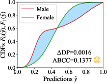
Existing group fairness notions require algorithms to treat different groups equally, and the degree of fairness violation is usually measured via the dissimilarity of model predictions. For example, Demographic Parity (DP) requires model predictions to be independent of sensitive attributes (Dwork et al., 2012; Kamishima et al., 2012; Jiang et al., 2020). To measure the violation of DP, most of existing works adopt metric, which calculates the difference in average predictions between the two demographic groups (Zemel et al., 2013; Chuang & Mroueh, 2021; Li et al., 2023b). However, since having the same values in average predictions between the two groups cannot ensure that the distributions are also the same, we argue that the widely used may fail to detect the violation of demographic parity. Figure 1(a) illustrates a toy example where the red and green curves represent the Cumulative Distribution Function (CDF) for the male and female groups, respectively. Despite the small , it is clear that the prediction distribution is not independent of gender as a sensitive attribute, with males more likely to be assigned extremely small and large predictive probabilities, while females are more concentrated in the middle-sized probabilities. To show the limitation of , we further calculate the Area Between CDF Curves () to measure the total variation between CDFs (Han et al., 2023a), which demonstrates significantly greater differences between groups.
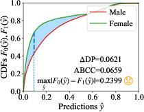
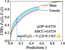
Moreover, as most of the existing metrics measure the overall disparity along all possible predictions, they fail to capture the local disparity at or around certain predictions. As a matter of fact, different metric values do not imply the relative magnitude of extreme local disparities. For example, although both and values of predictions in Figure 1(b) is better than those in Figure 1(c), its CDF disparity along predictions is less uniform, resulting in much more serious maximal disparity (). Generally, a pre-defined threshold is used to make a binary decision based on model predictions, where varying thresholds lead to changing proportions of positive decisions of different groups (Chen & Wu, 2020). If the decision threshold takes the value where the maximal CDF disparity is achieved, the group unfairness would be seriously exacerbated (e.g., the difference of group positive proportion in Figure 1(b) will be up to nearly 24%). Therefore, it’s important to capture and measure the extreme local disparity, which is yet prone to be “averaged” by overall variation of previous fairness metrics.
To address the limitations of previous fairness metrics, we propose a novel fairness metric called Maximal Cumulative ratio Disparity along varying Predictions’ -neighborhood, denoted as , whose core idea is calculating the maximal local disparity of the CDFs of two demographic groups. Considering that vast of predictions falling in a small prediction interval may result in sharp distribution changes, we firstly replace the exact CDF disparity at each prediction as the minimal disparity within its -neighborhood. In this way, the group disparity along varying predictions becomes smoother, thus the metric value becomes more robust to sharp distributions. We also theoretically prove several properties of the proposed metric, including but not limited to its monotonicity w.r.t. , and its relationship with previous fairness metrics.
Furthermore, given the model predictions for real instances in two demographic groups, we adopt empirical distribution function as the estimated CDF, and further propose two algorithms which exactly and approximately calculate the empirical metric value, respectively. Specifically, the approximation algorithm can greatly reduce the computational complexity with low value error. To train a fair classifier in view of maximal local disparity, we firstly adopt a differentiable approximation of CDF disparity based on temperature sigmoid function (Han & Moraga, 1995), and then minimize the maximal estimated CDF disparity using the bi-level optimization approach (Ji et al., 2021). In this way, the distribution disparity becomes more uniform (Figure 1(c)), further approaching demographic parity.
The contributions of this paper are summarized as follows:
We propose a novel fairness metric called to measure the maximal local disparity of a classifier, and derive several theoretical properties about the metric.
To empirically estimate with finite instances, we propose an exact and an approximate calculation algorithm, where the approximate algorithm greatly reduces computational complexity with low estimation error.
We further develop a bi-level optimization algorithm using differentiable approximation of to train a fair classifier which minimizes the maximal local disparity.
Experiments on tabular and image datasets (Adult, Bank and CelebA) demonstrate that our learning algorithm can effectively achieve better fairness-accuracy trade-offs.
2 Preliminaries
2.1 Demographic Parity and Measurements
Without loss of generality, we consider the binary classification task where each instance consists of an input , a class label and a group label , which is defined by sensitive attributes such as gender, age or race. We focus on demographic parity which requires the model’s predictive probabilities to be independent of the group label , where is a classifier with model parameter . To measure the model’s fairness violation, the following metric calculates the average prediction difference of two groups
where denotes the distributions of instances in two groups. In addition, given a finite dataset with samples and model predictions with , the empirical estimation of can be obtained as
where is the index set of instances in two groups. Apart from the widely-used () metric111To improve the notation briefness, we omit the arguments and , e.g., is short for . which measures unfairness in expectation-level, recent work (Han et al., 2023a) proposes a distribution-level metric called as follows
where and () are the CDFs of model predictions of instances from and
Similar to , the estimated value using can be computed as follows
where and are the empirical distribution functions of model predictions of instances in two groups
| (1) |
and denotes the indicator function.
2.2 Discussions about Previous Metrics
Drawbacks of . Although has become the de facto fairness criterion in previous literatures, it is insufficient to measure the violation of demographic parity. The reason is that does not indicate identical distributions of group prediction, thus the independency of predictions and group labels cannot be guaranteed. As shown in Figure 1(a), the distribution gap between the two groups is evident despite is very close to .
Drawbacks of . Unlike , is a necessary and sufficient condition for establishing demogarphic parity. However, as value cannot reflect the local distribution disparity, it fails to accurately measure the degree of unfairness in cases where extreme local disparity is emphasized. For example, although the maximal disparity in Figure 1(c) () is much smaller than that of Figure 1(b) (), its value is misleadingly larger (i.e., ).
Summary. Previous expectation-level and distribution-level metrics tend to average the extreme but important local disparity through overall calculation, thus their values cannot accurately measure the fairness violation in certain cases. This enlighten us to develop new fairness metrics to capture the maximal local disparity of classifiers.
3 The Proposed Metric
In this section, we propose a novel fairness metric called to measure the maximal local disparity of classifiers, and provide theoretical properties, estimation algorithms and an optimization framework about the metric. All the proofs of the theorems can be referred in Appendix A.
3.1 Metric
Denote the absolute difference of the two groups’ CDFs of model predictions as . To capture the worst case that a classifier violates demographic parity, an intuitive idea is to calculate the Maximal Cumulative ratio Disparity along varying Predictions using
| (2) |
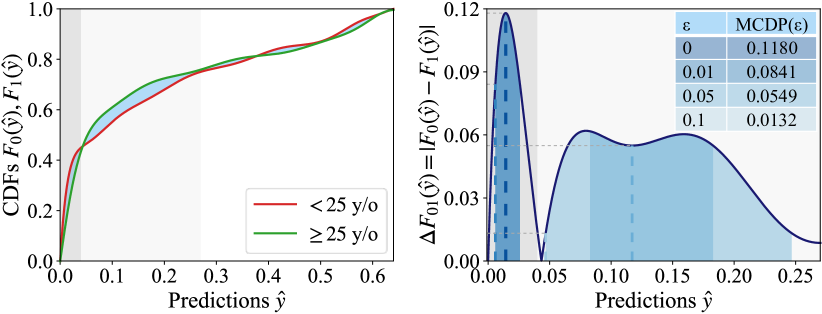
As only focuses on the maximal disparity, it serves as a more rigorous fairness measurement compared with previous metrics. However, it is susceptible to extremely sharp distributions within certain intervals. As an example shown in Figure 2, the value is large () due to a large number of instances with predictions around , which may misleadingly reflect the unfairness. To address this issue, we introduce a local measurement to smooth . For a specific prediction point , we take the minimal disparity within its -neighborhood as the maximal local disparity instead of the exact disparity . In this way, we slightly modify Eq. (2) to compute the Maximal Cumulative ratio Disparity along varying Predictions’ -neighborhood as
| (3) |
can also be interpreted as the maximum of the minimal CDF disparity of any prediction intervals with length (or if endpoints or is included). In particular, as the zero length interval degenerates to a point, degenerates to in Eq. (2).
3.2 Theoretical Analysis of
We derive several properties of metric as below:
Theorem 3.1 (Properties of ).
The proposed metric has the following desired properties: ① has a range of . ② holds if and only if demographic parity is established. ③ is invariant to any monotone and invertible transformation . ④ is a monotonically decreasing function w.r.t. . ⑤ Assume is continuous on with Lipschitz constant (Goldstein, 1977), then
Remarks. Properties ② and ③ show that satisfies the sufficiency and fidelity criteria for fairness measurement (Han et al., 2023a). A visualized interpretation of property ④ can be referred in Figure 2, where wider intervals (i.e., larger values) lead to smaller values. Property ⑤ provides an upper bound of the metric with given values, which also suggests that the distribution-level disparity can be controlled by minimizing the maximal local disparity.
3.3 Estimating the Metric
In real-world settings where algorithmic fairness is evaluated on finite data samples, we adopt the empirical distribution function as the estimated CDF. Formally, the empirical metric estimated over can be written as
| (4) |
where . By the Glivenko-Cantelli theorem (Tucker, 1959), the estimated metric value above converges to the true metric value in Eq. (3) almost surely with increasing sample size (see Appendix B for formal proofs), which demonstrates that serves as a preferable estimation of .
However, it is intractable to traverse all possible values in and values in ’s -neighborhood, which poses a challenge to compute the metric in Eq. (4). Nevertheless, thanks to the step-like pattern’s property of the empirical distribution function, we can traverse finite and values. Based on different traversing strategies, we develop two algorithms which calculates the exact and approximate value of , respectively. The exact algorithm only traverses predictions of instances in (lines 7-10 in Algorithm 1). In contrast, the approximate algorithm firstly samples prediction points that are equally spaced by on , where is a pre-defined hyper-parameter to control the sampling frequency. Afterwards, it traverses consecutive sampled points to estimate the maximal local disparity (lines 4-5 in Algorithm 2). Notably, the two algorithms have the following properties:
Theorem 3.2 (Exactness).
Theorem 3.3 (Over-estimation).
The value returned by Algorithm 2 never underestimates the true metric value, i.e., .
Theorem 3.4 (Monotonicity w.r.t. sampling frequency).
Denote as the value returned by Algorithm 2 with sampling frequency . For any , we have .
Computational Complexity. The calculation process of Algorithms 1 and 2 are mainly based on specific traverse strategies on and in Eq. (4). As the exact algorithm needs to traverse instances in twice (lines 7-9 in Algorithm 1), its computational complexity is . As to the approximate algorithm, the complexity of traversing sampled prediction points (line 4 in Algorithm 2) is , and the complexity of finding the minimal CDF disparity in each consecutive points is . Therefore, the overall computational complexity is . More detailed analysis can be referred in Appendix C. In practice, as can be set with very small values (i.e., ), the computational complexity of the approximate algorithm is greatly reduced compared to the exact algorithm.
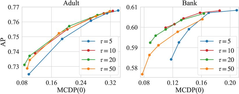
More Discussions about . As discussed before, increasing values would boost the computational complexity of Algorithm 2. On the flip side, according to Theorems 3.3 and 3.4, the estimation error would keep decreasing as increases, indicating a trade-off between efficiency and accuracy. In practice, both estimation accuracy and efficiency can achieve promising results with varying values.
3.4 DiffMCDP: Bi-Level Optimization Algorithm
Based on previous analysis, it is essential to train a fair classifier which minimizes the maximal local disparity to approach demographic parity. According to property ⑤ in Theorem 3.1, we can minimize as an upper bound of for any . A natural idea is to impose the metric as a regularization term on the classification loss. However, as the empirical distribution functions are not differentiable w.r.t. model parameter , directly regularizing is implausible. To address this issue, we firstly estimate in a differentiable way
where is a variant of sigmoid function with temperature as a hyper-parameter (Han & Moraga, 1995). Notably, when the temperature tends to infinity, we have converges to the as follows.
Theorem 3.5.
as .
With the differentiable estimation above, the fairness-regularized objective function can be written as
| (5) |
where denotes the classification loss for , and controls the trade-off between accuracy and fairness. To solve Eq. (5), we adopt the bi-level optimization approach – firstly find the prediction which achieves the maximal CDF disparity as , and then find the optimal model parameter by . We provide the detailed learning algorithm in Algorithm 3.
4 Experiments
Datasets and Backbone Models. In our experiments, we adopt two tabular datasets and one image dataset for evaluation: ① Adult (Kohavi, 1996) is a popular UCI dataset which contains personal information of over 40K individuals from US 1994 census data. The task is to predict whether a person’s annual income is over $50K or not, and we treat gender as the sensitive attribute. ② Bank (Moro et al., 2014) dataset is collected from a Portuguese banking institution’s marketing campaigns, and its goal is to predict whether a client will make a deposit subscription or not. We take age as the sensitive attribute (whether the age is over 25 or not). ③ CelebA (Liu et al., 2015) dataset contains over 20K face images of celebrities, where each image has 40 human-labeled binary face attributes. We use gender as the sensitive attribute, and choose attractive face and wavy hair as target attributes to create two meta-datasets, denoted as CelebA-A and CelebA-W respectively. For tabular datasets, we adopt a two-layer multi-layer perceptron as the backbone model. For CelebA-A and CelebA-W, we use ResNet-18 (He et al., 2016) initialized with pretrained weights.
Baselines and Evaluation Protocols. We compare our proposed method (denoted as DiffMCDP) with the following baselines: ① ERM trains the model with the vanilla classification loss without fairness objectives. ② AdvDebias (Zhang et al., 2018) minimizes the adversary’s ability of inferring sensitive attributes from model representations. ③ DiffDP imposes the metric as a regularization term on the empirical risk. ④ FairMixup (Chuang & Mroueh, 2021) regularizes models on interpolated distributions between two groups. ⑤ DRAlign (Li et al., 2023b) uses gradient-guided parity alignment to encourage gradient-weighted consistency of neurons across groups. ⑥ DiffABCC regularizes the metric on the empirical risk. We use average precision () to evaluate the classification accuracy, and use , , and to measure the algorithmic fairness. More implementation details can be referred in Appendix D.
4.1 Performance Comparison
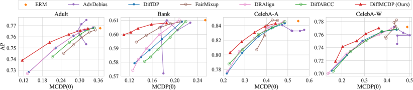
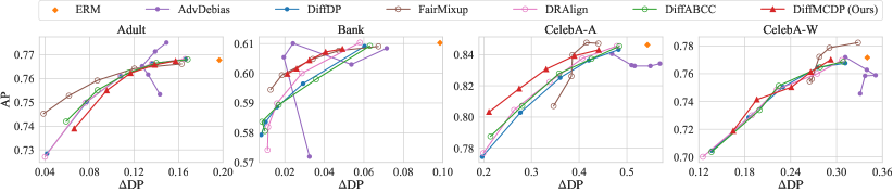
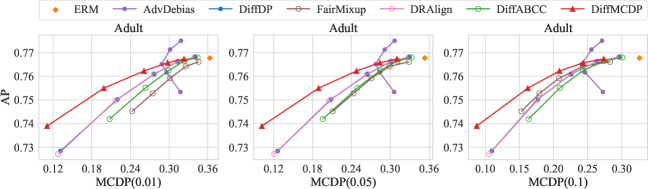
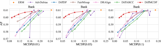
Figure 3 shows the trade-off relationships between and of baselines and our proposed method. We can observe that DiffMCDP consistently outperforms other baselines in terms of fairness-accuracy trade-offs across all datasets, which suggests that our proposed fair training algorithm can effectively reduce maximal local disparity to improve fairness. In addition, traditional fair training algorithms can achieve desired trade-offs between accuracy and our proposed fairness metric. For example, the values of both DiffDP and DiffABCC decrease with increasing regularization strengths, which demonstrates that solely optimizing expectation-level or distribution-level metrics do contribute to minimizing the maximal local disparity. Nevertheless, they obtain inferior performance compared to DiffMCDP which directly regularizes , indicating their limitation in approaching demographic parity.
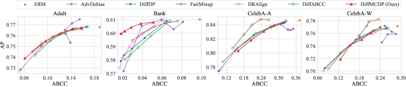
To explore the performance of our method under different fairness measurements, we report the values of , and metrics in Tables 1 and 2 (the trade-off curves can be referred in Appendix E.1). While DiffMCDP achieves the optimal results across various datasets, it also obtains comparable even superior or values compared to other baselines. For example, DiffMCDP achieves the lowest values in tabular datasets, and its values are optimal in two image datasets. These results illustrate that optimizing the maximal local disparity is also beneficial to improve both expectation-level and distribution-level fairness metrics.
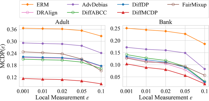
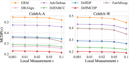
Lastly, we plot the changes of as varying local measurements in Figure 4 (the results of image datasets are deferred in Appendix E.2). From the figure, we can observe that DiffMCDP still consistently outperforms other baselines in terms of different variants of the metric. This validates the effectiveness of regularizing the upper bound of by in the training objective, demonstrating that our proposed framework is applicable to various scenarios with varying values. Additionally, it is noteworthy that the relative performance of other baselines changes with increasing values (e.g., there exists many intersection lines between 0.05 and 0.1 in Adult). This indicates that the relative fairness performance of various algorithms may change based on different manners of calculating local disparity, thus it’s essential to select varying values in for more comprehensive evaluation.
| Adult | Bank | |||||||
|---|---|---|---|---|---|---|---|---|
| ERM | 76.770.54 | 19.670.94 | 18.890.29 | 36.620.53 | 61.021.12 | 9.851.28 | 9.830.98 | 25.361.81 |
| AdvDebias | 76.520.62 | 12.731.81 | 12.951.35 | 29.282.26 | 60.541.02 | 1.952.76 | 3.950.97 | 17.524.12 |
| DiffDP | 75.020.28 | 7.771.20 | 8.970.73 | 22.371.11 | 58.361.67 | 1.030.23 | 2.130.20 | 14.011.34 |
| FairMixup | 74.520.40 | 3.871.20 | 7.340.62 | 24.871.53 | 59.451.94 | 1.280.44 | 2.950.91 | 13.222.91 |
| DRAlign | 74.980.28 | 7.641.22 | 8.860.75 | 22.081.19 | 58.191.54 | 1.150.41 | 1.980.23 | 13.581.26 |
| DiffABCC | 74.190.24 | 5.901.28 | 7.830.74 | 21.181.23 | 58.061.60 | 0.990.44 | 2.230.19 | 14.671.35 |
| DiffMCDP | 73.900.29 | 6.630.85 | 6.090.59 | 11.531.12 | 59.981.80 | 2.130.72 | 1.830.28 | 11.021.00 |
| CelebA-A | CelebA-W | |||||||
|---|---|---|---|---|---|---|---|---|
| ERM | 84.620.38 | 54.320.77 | 37.200.69 | 54.850.92 | 77.160.68 | 34.022.24 | 28.941.36 | 48.962.16 |
| AdvDebias | 84.040.51 | 46.901.89 | 30.722.05 | 47.451.83 | 77.190.47 | 31.141.44 | 25.272.48 | 43.115.20 |
| DiffDP | 82.520.42 | 36.031.77 | 21.331.40 | 36.401.61 | 75.041.60 | 23.010.95 | 16.991.29 | 29.173.00 |
| FairMixup | 80.701.03 | 34.643.23 | 14.151.63 | 35.522.67 | 75.450.72 | 26.494.48 | 17.961.04 | 39.613.01 |
| DRAlign | 80.451.05 | 26.362.48 | 15.251.71 | 27.382.46 | 74.861.49 | 22.201.54 | 16.951.11 | 29.162.76 |
| DiffABCC | 80.710.86 | 28.051.83 | 15.701.67 | 28.941.89 | 73.381.69 | 19.931.85 | 13.670.88 | 23.773.44 |
| DiffMCDP | 80.320.67 | 21.101.94 | 16.031.61 | 23.101.66 | 74.141.26 | 19.581.91 | 15.351.26 | 20.291.78 |
4.2 Exact and Approximate Calculation
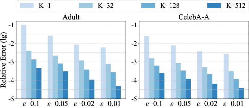
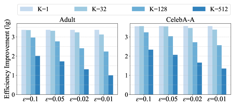
To explore the estimation accuracy and efficiency of the approximate algorithm on real-world data, we run both the exact and approximate algorithms with varying and values to compute of the testing results in Figure 3. Then we calculate the relative error by , where and are the estimated metric value returned by the exact and approximate algorithms, respectively. Moreover, we measure the efficiency improvement by , where and represents the time of a single run of the exact and approximate algorithms.
We plot the results across different settings in Figure 5 (results on more datasets are deferred in Appendix E.3), where we have the following observations. ① With increasing values, the relative error decreases as Theorems 3.3 and 3.4 suggests. Meanwhile, the calculation time also increases, which is consistent with the positive correlation between computational complexity and sampling frequency. It is noteworthy that selecting moderate values can achieve promising performance. For example, when , the average estimation error and efficiency improvement are and over times, respectively. ② As increases, the calculation efficiency improvement over the exact algorithm keeps increasing, which can be explained by the inverse correlation between computational complexity and . Meantime, the relative error also increases, and a potential reason is that estimating the minimal CDF value with sampled prediction points within a larger interval tends to be more inaccurate. ③ The efficiency improvements are more obvious in CelebA-A dataset compared with Adult dataset, which is attributed to that the number of instances in CelebA-A is larger than Adult, and the computational complexity of the exact algorithm is quadratically proportional to the sample size. This indicates that the efficiency superiority of approximation algorithm becomes more evident when adopted to predictions on more instances.
4.3 In-Depth Analysis
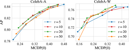
Effect of Temperature . The temperature in Algorithm 3 is crucial to approximate the true maximal CDF disparity. On the one hand, as shown in Theorem 3.5, the estimation error vanishes when the temperature grows. On the other hand, in practice, a large value may arise the gradient vanishing problem (Roodschild et al., 2020), which limits the learning capacity and optimization convergence. To verify this point, we tune in and plot the fairness-accuracy trade-off curves as shown in Figure 6 (the results of image datasets are deferred in Appendix E.4). We find that very small or large temperatures () may lead to dissatisfactory results, thus it’s better to adopt moderate temperatures () to effectively trade-off the estimation accuracy and the gradient magnitude.
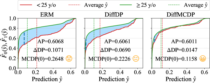
Visualizations of Model Predictions. Figure 7 visualizes the empirical distribution functions of model predictions for two age groups in Bank dataset, where the training methods include ERM, DiffDP and DiffMCDP. As ERM optimizes the vanilla classification loss without fairness objectives, its prediction distribution gap is the most evident. Taking a step further, DiffDP regularizes the metric on empirical risk, thus the average prediction gap is much smaller than ERM. Nevertheless, it leaves a lot to be desired in terms of reducing the maximal local disparity. By contrast, our proposed DiffMCDP method is much more effective in narrowing the maximal gap between prediction distributions, i.e., the value of DiffMCDP declined by compared to DiffDP, which is also beneficial for minimizing the difference of average predictions.
5 Related Work
Fairness Notions and Metrics. While machine learning algorithms are widely-used in high-stake applications with broad social impacts, algorithmic fairness has been a crucial requirement in accessing and regulating the models (Yeung, 2018; Chen et al., 2019). Generally, algorithmic fairness notions can be categorized into group fairness (Feldman et al., 2015; Shui et al., 2022; Sun et al., 2023; Jin et al., 2024), individual fairness (Dwork et al., 2012; Biega et al., 2018; Li et al., 2023a; Wicker et al., 2023) and counterfactual fairness (Kusner et al., 2017; Chiappa, 2019; Wu et al., 2019; Ma et al., 2022; Han et al., 2023b; Rosenblatt & Witter, 2023). Group fairness requires the model to treat different groups specified by certain sensitive attributes equally without discrimination. For example, demographic parity (Zemel et al., 2013; Jiang et al., 2020; Fukuchi & Sakuma, 2023) defines fairness as the independence of model predictions and sensitive attributes, while equalized odds (Hardt et al., 2016) requires the prediction and group membership to be independent conditioned on the target label.
To measure the degree of fairness violation, various fairness metrics have been adopted for model evaluation (Garg et al., 2020; Franklin et al., 2022; Han et al., 2024). Specifically, to measure the violation of demographic parity, (Zemel et al., 2013) calculates the difference of average model predictions of instances in two demographic groups; -Rule (Zafar et al., 2017b) computes the ratio between probabilities of two groups assigned the positive decision outcome; (Jiang et al., 2020) averages the binary group prediction’s disparity over 100 uniformly-spaced thresholds; and (Han et al., 2023a) measures the difference between the prediction distribution for different groups. In this work, we point out that these expectation-level or distribution-level metrics may fail to measure unfairness in certain cases, since the extreme but important local disparity is prone to be averaged by overall variation.
Fair Machine Learning Algorithms. To alleviate unfairness of machine learning systems, various fairness-aware algorithms have been proposed, which can be generally divided into three categories: pre-processing methods (Kamiran & Calders, 2012; Calmon et al., 2017; Zhang et al., 2018; Biswas & Rajan, 2021) attempt to adjust the training data distribution to remove the underlying data bias; in-processing methods (Kamishima et al., 2012; Zafar et al., 2017a, b; Chuang & Mroueh, 2021; Roh et al., 2021) aim to reduce model’s intrinsic discrimination during the training stage; and post-processing (Hardt et al., 2016; Pleiss et al., 2017; Noriega-Campero et al., 2019; Chen et al., 2024; Yin et al., 2024) methods perform calibration on model predictions after the training. Among these three categories, in-processing methods fundamentally improve the fairness of both model outputs and representations, which can also lead to the highest utility (Barocas et al., 2023; Wan et al., 2023). Recently, there is also a line of works focusing on how to achieve algorithmic fairness in special cases, for instance, fairness under distributional shift (Chai & Wang, 2022; Jiang et al., 2023; Roh et al., 2023) or with missing attribute values (Zhao et al., 2022; Feng et al., 2023; Zhu et al., 2023). Nevertheless, it is unknown that whether these algorithms can improve fairness in terms of reducing maximal local disparity or not, and this work re-evaluates some of the methods on benchmark datasets.
6 Conclusions and Future Work
In this work, we reveal that previous expectation-level fairness metrics () cannot accurately measure the violation of demographic parity. Meanwhile, the overall variation of distribution-level metrics () may conceal the extreme but important local disparity. Upon this understanding, we propose a novel metric called , which calculates the maximal local disparity (defined by the minimal CDF disparity of a prediction’s -neighborhood) of two demographic groups. Accordingly, we propose two algorithms to estimate with finite samples, where the approximate algorithm greatly reduces the computational complexity with high accuracy compared to the exact one. Furthermore, we develop a fair model learning framework which regularizes a differentiable estimation of . Extensive experiments are conducted on both tabular and image datasets demonstrate the effectiveness of our proposal.
In the future, we plan to extend the metric to measure the unfairness in terms of other fairness notions, such as equalized odds (Hardt et al., 2016) and demographic parity over multiple or continuous attributes (Jiang et al., 2022; Grari et al., 2024). Moreover, designing more effective fair learning algorithms to control the maximal local disparity is also a interesting and promising research direction.
Acknowledgement
This work was supported in part by National Natural Science Foundation of China (No. 623B2002 and 62272437) and the CCCD Key Lab of Ministry of Culture and Tourism.
Impact Statement
Fairness is a crucial issue when designing trustworthy machine learning systems. Recent years have witnessed many impressive works which aims at developing fair machine learning algorithms under various scenarios. In this paper, by noticing the gap between overall distribution disparity (which is the core of traditional fairness measurements) and local disparity, we propose a novel fairness metric called , which captures the maximal local disparity of model predictions on two demographic groups. Compared with previous metrics such as and , is more strict and conservative in measuring the violation of demographic parity, which is beneficial for reducing the risk of discrimination and improving algorithmic fairness when developing high-stake applications. We call on the research community to investigate more rigorous and theoretically-guaranteed fairness evaluation protocols, which can advance the field of trustworthy machine learning.
References
- Barocas et al. (2023) Barocas, S., Hardt, M., and Narayanan, A. Fairness and Machine Learning: Limitations and Opportunities. MIT Press, 2023.
- Berk et al. (2021) Berk, R., Heidari, H., Jabbari, S., Kearns, M., and Roth, A. Fairness in Criminal Justice Risk Assessments: The State of the Art. Sociological Methods & Research, 50(1):3–44, 2021.
- Biega et al. (2018) Biega, A. J., Gummadi, K. P., and Weikum, G. Equity of Attention: Amortizing Individual Fairness in Rankings. In The 41st International ACM SIGIR Conference on Research & Development in Information Retrieval, pp. 405–414, 2018.
- Bishop (1995) Bishop, C. M. Neural Networks for Pattern Recognition. Oxford University Press, 1995.
- Biswas & Rajan (2021) Biswas, S. and Rajan, H. Fair Preprocessing: Towards Understanding Compositional Fairness of Data Transformers in Machine Learning Pipeline. In Proceedings of the 29th ACM Joint Meeting on European Software Engineering Conference and Symposium on the Foundations of Software Engineering, pp. 981–993, 2021.
- Boyd & Vandenberghe (2004) Boyd, S. P. and Vandenberghe, L. Convex Optimization. Cambridge University Press, 2004.
- Calmon et al. (2017) Calmon, F., Wei, D., Vinzamuri, B., Natesan Ramamurthy, K., and Varshney, K. R. Optimized Pre-Processing for Discrimination Prevention. Advances in Neural Information Processing Systems, 30, 2017.
- Chai & Wang (2022) Chai, J. and Wang, X. Fairness with Adaptive Weights. In International Conference on Machine Learning, pp. 2853–2866. PMLR, 2022.
- Chen et al. (2019) Chen, J., Kallus, N., Mao, X., Svacha, G., and Udell, M. Fairness under Unawareness: Assessing Disparity When Protected Class Is Unobserved. In Proceedings of the Conference on Fairness, Accountability, and Transparency, pp. 339–348, 2019.
- Chen & Wu (2020) Chen, M. and Wu, M. Towards Threshold Invariant Fair Classification. In Conference on Uncertainty in Artificial Intelligence, pp. 560–569. PMLR, 2020.
- Chen et al. (2024) Chen, W., Klochkov, Y., and Liu, Y. Post-hoc Bias Scoring Is Optimal For Fair Classification. In International Conference on Learning Representations, 2024.
- Chiappa (2019) Chiappa, S. Path-Specific Counterfactual Fairness. Proceedings of the AAAI conference on artificial intelligence, 33(01):7801–7808, 2019.
- Chuang & Mroueh (2021) Chuang, C.-Y. and Mroueh, Y. Fair Mixup: Fairness via Interpolation. In International Conference on Learning Representations, 2021.
- Chung & Erdös (1952) Chung, K. L. and Erdös, P. On the Application of the Borel-Cantelli Lemma. Transactions of the American Mathematical Society, 72(1):179–186, 1952.
- Creager et al. (2019) Creager, E., Madras, D., Jacobsen, J.-H., Weis, M., Swersky, K., Pitassi, T., and Zemel, R. Flexibly Fair Representation Learning by Disentanglement. In International Conference on Machine Learning, pp. 1436–1445. PMLR, 2019.
- Dai & Wang (2021) Dai, E. and Wang, S. Say No to the Discrimination: Learning Fair Graph Neural Networks with Limited Sensitive Attribute Information. In Proceedings of the 14th ACM International Conference on Web Search and Data Mining, pp. 680–688, 2021.
- Dutta et al. (2020) Dutta, S., Wei, D., Yueksel, H., Chen, P.-Y., Liu, S., and Varshney, K. Is There a Trade-off between Fairness and Accuracy? A Perspective Using Mismatched Hypothesis Testing. In International Conference on Machine Learning, pp. 2803–2813. PMLR, 2020.
- Dwork et al. (2012) Dwork, C., Hardt, M., Pitassi, T., Reingold, O., and Zemel, R. Fairness through Awareness. In Proceedings of the 3rd Innovations in Theoretical Computer Science Conference, pp. 214–226, 2012.
- Faliagka et al. (2012) Faliagka, E., Ramantas, K., Tsakalidis, A., and Tzimas, G. Application of Machine Learning Algorithms to an Online Recruitment System. In International Conference on Internet and Web Applications and Services, pp. 215–220, 2012.
- Feldman et al. (2015) Feldman, M., Friedler, S. A., Moeller, J., Scheidegger, C., and Venkatasubramanian, S. Certifying and Removing Disparate Impact. In Proceedings of the 21th ACM SIGKDD International Conference on Knowledge Discovery and Data Mining, pp. 259–268, 2015.
- Feng et al. (2023) Feng, R., Calmon, F. P., and Wang, H. Adapting Fairness Interventions to Missing Values. Advances in Neural Information Processing Systems, 2023.
- Franklin et al. (2022) Franklin, J. S., Bhanot, K., Ghalwash, M., Bennett, K. P., McCusker, J., and McGuinness, D. L. An Ontology for Fairness Metrics. In Proceedings of the 2022 AAAI/ACM Conference on AI, Ethics, and Society, pp. 265–275, 2022.
- Fukuchi & Sakuma (2023) Fukuchi, K. and Sakuma, J. Demographic Parity Constrained Minimax Optimal Regression under Linear Model. Advances in Neural Information Processing Systems, 2023.
- Garg et al. (2020) Garg, P., Villasenor, J., and Foggo, V. Fairness Metrics: A Comparative Analysis. In 2020 IEEE International Conference on Big Data, pp. 3662–3666. IEEE, 2020.
- Goldstein (1977) Goldstein, A. Optimization of Lipschitz Continuous Functions. Mathematical Programming, 13:14–22, 1977.
- Graham et al. (1989) Graham, R. L., Knuth, D. E., Patashnik, O., and Liu, S. Concrete Mathematics: A Foundation for Computer Science. Computers in Physics, 3(5):106–107, 1989.
- Grari et al. (2024) Grari, V., Laugel, T., Hashimoto, T., Lamprier, S., and Detyniecki, M. On the Fairness ROAD: Robust Optimization for Adversarial Debiasing. In International Conference on Learning Representations, 2024.
- Han & Moraga (1995) Han, J. and Moraga, C. The Influence of the Sigmoid Function Parameters on the Speed of Backpropagation Learning. In International Workshop on Artificial Neural Networks, pp. 195–201. Springer, 1995.
- Han et al. (2023a) Han, X., Jiang, Z., Jin, H., Liu, Z., Zou, N., Wang, Q., and Hu, X. Retiring : New Distribution-Level Metrics for Demographic Parity. Transactions on Machine Learning Research, 2023a.
- Han et al. (2023b) Han, X., Zhang, L., Wu, Y., and Yuan, S. Achieving Counterfactual Fairness for Anomaly Detection. In Pacific-Asia Conference on Knowledge Discovery and Data Mining, pp. 55–66. Springer, 2023b.
- Han et al. (2024) Han, X., Chi, J., Chen, Y., Wang, Q., Zhao, H., Zou, N., and Hu, X. Ffb: A Fair Fairness Benchmark for In-Processing Group Fairness Methods. In International Conference on Learning Representations, 2024.
- Hardt et al. (2016) Hardt, M., Price, E., and Srebro, N. Equality of Opportunity in Supervised Learning. Advances in Neural Information Processing Systems, 29, 2016.
- He et al. (2016) He, K., Zhang, X., Ren, S., and Sun, J. Deep Residual Learning for Image Recognition. In Proceedings of the IEEE Conference on Computer Vision and Pattern Recognition, pp. 770–778, 2016.
- Jacobs & Wallach (2021) Jacobs, A. Z. and Wallach, H. Measurement and Fairness. In Proceedings of the 2021 ACM Conference on Fairness, Accountability, and Transparency, pp. 375–385, 2021.
- Ji et al. (2021) Ji, K., Yang, J., and Liang, Y. Bilevel Optimization: Convergence Analysis and Enhanced Design. In International Conference on Machine Learning, pp. 4882–4892. PMLR, 2021.
- Jiang et al. (2020) Jiang, R., Pacchiano, A., Stepleton, T., Jiang, H., and Chiappa, S. Wasserstein Fair Classification. In Uncertainty in Artificial Intelligence, pp. 862–872. PMLR, 2020.
- Jiang et al. (2022) Jiang, Z., Han, X., Fan, C., Yang, F., Mostafavi, A., and Hu, X. Generalized Demographic Parity for Group Fairness. In International Conference on Learning Representations, 2022.
- Jiang et al. (2023) Jiang, Z., Han, X., Jin, H., Wang, G., Chen, R., Zou, N., and Hu, X. Chasing Fairness under Distribution Shift: A Model Weight Perturbation Approach. Advances in Neural Information Processing Systems, 2023.
- Jin et al. (2024) Jin, J., Li, H., Feng, F., Ding, S., Wu, P., and He, X. Fairly Recommending with Social Attributes: A Flexible and Controllable Optimization Approach. Advances in Neural Information Processing Systems, 36, 2024.
- Jung et al. (2023) Jung, S., Park, T., Chun, S., and Moon, T. Re-Weighting Based Group Fairness Regularization via Classwise Robust Optimization. In International Conference on Learning Representations, 2023.
- Kamiran & Calders (2012) Kamiran, F. and Calders, T. Data Preprocessing Techniques for Classification without Discrimination. Knowledge and Information Systems, 33(1):1–33, 2012.
- Kamishima et al. (2012) Kamishima, T., Akaho, S., Asoh, H., and Sakuma, J. Fairness-Aware Classifier with Prejudice Remover Regularizer. In Machine Learning and Knowledge Discovery in Databases: European Conference, pp. 35–50. Springer, 2012.
- Kohavi (1996) Kohavi, R. Scaling up the Accuracy of Naive-Bayes Classifiers: A Decision-Tree Hybrid. In Proceedings of the 2nd International Conference on Knowledge Discovery and Data Mining, volume 96, pp. 202–207, 1996.
- Kusner et al. (2017) Kusner, M. J., Loftus, J., Russell, C., and Silva, R. Counterfactual Fairness. Advances in Neural Information Processing Systems, 30, 2017.
- Li et al. (2023a) Li, P., Xia, E., and Liu, H. Learning Antidote Data to Individual Unfairness. In International Conference on Machine Learning, pp. 20168–20181. PMLR, 2023a.
- Li et al. (2023b) Li, T., Guo, Q., Liu, A., Du, M., Li, Z., and Liu, Y. FAIRER: Fairness as Decision Rationale Alignment. In International Conference on Machine Learning, pp. 19471–19489. PMLR, 2023b.
- Liu et al. (2015) Liu, Z., Luo, P., Wang, X., and Tang, X. Deep Learning Face Attributes in the Wild. In Proceedings of the IEEE International Conference on Computer Vision, pp. 3730–3738, 2015.
- Ma et al. (2022) Ma, J., Guo, R., Wan, M., Yang, L., Zhang, A., and Li, J. Learning Fair Node Representations with Graph Counterfactual Fairness. In Proceedings of the 15th ACM International Conference on Web Search and Data Mining, pp. 695–703, 2022.
- Mehrabi et al. (2021) Mehrabi, N., Morstatter, F., Saxena, N., Lerman, K., and Galstyan, A. A Survey on Bias and Fairness in Machine Learning. ACM Computing Surveys (CSUR), 54(6):1–35, 2021.
- Moro et al. (2014) Moro, S., Cortez, P., and Rita, P. A Data-Driven Approach to Predict the Success of Bank Telemarketing. Decision Support Systems, 62:22–31, 2014.
- Mukerjee et al. (2002) Mukerjee, A., Biswas, R., Deb, K., and Mathur, A. P. Multi-Objective Evolutionary Algorithms for the Risk-Return Trade-off in Bank Loan Management. International Transactions in Operational Research, 9(5):583–597, 2002.
- Nair & Hinton (2010) Nair, V. and Hinton, G. E. Rectified Linear Units Improve Restricted Boltzmann Machines. In International Conference on Machine Learning, pp. 807–814. PMLR, 2010.
- Noriega-Campero et al. (2019) Noriega-Campero, A., Bakker, M. A., Garcia-Bulle, B., and Pentland, A. Active Fairness in Algorithmic Decision Making. Proceedings of the 2019 AAAI/ACM Conference on AI, Ethics, and Society, pp. 77–83, 2019.
- Paszke et al. (2019) Paszke, A., Gross, S., Massa, F., Lerer, A., Bradbury, J., Chanan, G., Killeen, T., Lin, Z., Gimelshein, N., Antiga, L., et al. Pytorch: An Imperative Style, High-Performance Deep Learning Library. Advances in Neural Information Processing Systems, 32, 2019.
- Pleiss et al. (2017) Pleiss, G., Raghavan, M., Wu, F., Kleinberg, J., and Weinberger, K. Q. On Fairness and Calibration. Advances in Neural Information Processing Systems, 30, 2017.
- Raghavan et al. (2020) Raghavan, M., Barocas, S., Kleinberg, J., and Levy, K. Mitigating Bias in Algorithmic Hiring: Evaluating Claims and Practices. In Proceedings of the 2020 Conference on Fairness, Accountability, and Transparency, pp. 469–481, 2020.
- Roh et al. (2021) Roh, Y., Lee, K., Whang, S. E., and Suh, C. FairBatch: Batch Selection for Model Fairness. In International Conference on Learning Representations, 2021.
- Roh et al. (2023) Roh, Y., Lee, K., Whang, S. E., and Suh, C. Improving Fair Training under Correlation Shifts. In International Conference on Machine Learning, pp. 29179–29209. PMLR, 2023.
- Roodschild et al. (2020) Roodschild, M., Gotay Sardiñas, J., and Will, A. A New Approach for the Vanishing Gradient Problem on Sigmoid Activation. Progress in Artificial Intelligence, 9(4):351–360, 2020.
- Rosen (2007) Rosen, K. H. Discrete Mathematics and Its Applications. The McGraw Hill Companies, 2007.
- Rosenblatt & Witter (2023) Rosenblatt, L. and Witter, R. T. Counterfactual Fairness Is Basically Demographic Parity. Proceedings of the AAAI Conference on Artificial Intelligence, 37(12):14461–14469, 2023.
- Seabold & Perktold (2010) Seabold, S. and Perktold, J. Statsmodels: Econometric and Statistical Modeling with Python. In Proceedings of the 9th Python in Science Conference, volume 57, pp. 10–25080. Austin, TX, 2010.
- Shui et al. (2022) Shui, C., Xu, G., Chen, Q., Li, J., Ling, C. X., Arbel, T., Wang, B., and Gagné, C. On Learning Fairness and Accuracy on Multiple Subgroups. Advances in Neural Information Processing Systems, 35:34121–34135, 2022.
- Sun et al. (2023) Sun, R., Zhou, F., Dong, Z., Xie, C., Hong, L., Li, J., Zhang, R., Li, Z., and Li, Z. Fair-CDA: Continuous and Directional Augmentation for Group Fairness. Proceedings of the AAAI Conference on Artificial Intelligence, 37(8):9918–9926, 2023.
- Tolan et al. (2019) Tolan, S., Miron, M., Gómez, E., and Castillo, C. Why Machine Learning May Lead to Unfairness: Evidence from Risk Assessment for Juvenile Justice in Catalonia. In Proceedings of the 17th International Conference on Artificial Intelligence and Law, pp. 83–92, 2019.
- Tucker (1959) Tucker, H. G. A Generalization of the Glivenko-Cantelli Theorem. The Annals of Mathematical Statistics, 30(3):828–830, 1959.
- Wan et al. (2023) Wan, M., Zha, D., Liu, N., and Zou, N. In-Processing Modeling Techniques for Machine Learning Fairness: A Survey. ACM Transactions on Knowledge Discovery from Data, 17(3):1–27, 2023.
- Wick et al. (2019) Wick, M., Tristan, J.-B., et al. Unlocking Fairness: A Trade-off Revisited. Advances in Neural Information Processing Systems, 32, 2019.
- Wicker et al. (2023) Wicker, M., Piratia, V., and Weller, A. Certification of Distributional Individual Fairness. Advances in Neural Information Processing Systems, 2023.
- Wu et al. (2019) Wu, Y., Zhang, L., and Wu, X. Counterfactual Fairness: Unidentification, Bound and Algorithm. In Proceedings of the 28th International Joint Conference on Artificial Intelligence, 2019.
- Yeung (2018) Yeung, K. Algorithmic Regulation: A Critical Interrogation. Regulation & Governance, 12(4):505–523, 2018.
- Yin et al. (2024) Yin, T., Ton, J.-F., Guo, R., Yao, Y., Liu, M., and Liu, Y. Fair Classifiers that Abstain without Harm. In International Conference on Learning Representations, 2024.
- Zafar et al. (2017a) Zafar, M. B., Valera, I., Gomez Rodriguez, M., and Gummadi, K. P. Fairness beyond Disparate Treatment & Disparate Impact: Learning Classification without Disparate Mistreatment. In Proceedings of the 26th International Conference on World Wide Web, pp. 1171–1180, 2017a.
- Zafar et al. (2017b) Zafar, M. B., Valera, I., Rogriguez, M. G., and Gummadi, K. P. Fairness Constraints: Mechanisms for Fair Classification. In Artificial Intelligence and Statistics, pp. 962–970. PMLR, 2017b.
- Zemel et al. (2013) Zemel, R., Wu, Y., Swersky, K., Pitassi, T., and Dwork, C. Learning Fair Representations. In International Conference on Machine Learning, pp. 325–333. PMLR, 2013.
- Zhang et al. (2018) Zhang, B. H., Lemoine, B., and Mitchell, M. Mitigating Unwanted Biases with Adversarial Learning. In Proceedings of the 2018 AAAI/ACM Conference on AI, Ethics, and Society, pp. 335–340, 2018.
- Zhao et al. (2022) Zhao, T., Dai, E., Shu, K., and Wang, S. Towards Fair Classifiers without Sensitive Attributes: Exploring Biases in Related Features. In Proceedings of the Fifteenth ACM International Conference on Web Search and Data Mining, pp. 1433–1442, 2022.
- Zhu et al. (2023) Zhu, Z., Yao, Y., Sun, J., Li, H., and Liu, Y. Weak Proxies Are Sufficient and Preferable for Fairness with Missing Sensitive Attributes. In International Conference on Machine Learning, pp. 43258–43288. PMLR, 2023.
Appendix
Appendix A Proofs
A.1 Proofs of Theorem 3.1
Theorem 3.1 (Properties of ). The proposed metric has the following desired properties: ① has a range of . ② holds if and only if demographic parity is established. ③ is invariant to any monotone and invertible transformation on . ④ is a monotonically decreasing function w.r.t. . ⑤ Assume is continuous on with Lipschitz constant (Goldstein, 1977), then
Proof.
① If demographic parity is established, i.e., , then . In addition, let and , we have . This proves that .
② According to Eq. (3), can be written as
Thus the following holds
which indicates that and demographic parity are equivalent.
③ Denote the prediction which achieves the largest value as . Moreover, denote the CDFs for the transformed predictions in two groups as and . As is a monotone and invertible transformation on , for any , there exists , such that . Thus we have
and the equal sign holds if and only if . This indicates that is invariant to .
④ For any and , we have
which yields that . ∎
⑤ To complete the proof of Property ⑤, we firstly present and prove the following two lemmas:
Lemma A.1.
If is continuous on with Lipschitz constant , then .
Lemma A.2.
If is continuous on with Lipschitz constant , then .
To complete the proof of Lemma A.1, we first give some useful lemmas (which is based on ) below.
Lemma A.3.
Let , then and .
Proof.
Firstly, we note that the following holds
Thus Furthermore, for any , by Lipschitz continuity, we have
| (6) |
which yields that
∎
Lemma A.4.
For any such that , .
Proof.
Lemma A.5.
For any such that (where is defined as Lemma A.3 stated), there exists such that and .
Proof.
Assume to the contrary that there exists , such that and one of the following satisfies. (i) If , let and , we have and . Thus the value should satisfy that
| (7) |
(ii) If , let and . Similar to (i), we have
| (8) |
The fact that at least one of Eq. (7) and Eq. (8) holds derives that , which contradicts with . Therefore, the original assumption must be false, which completes the proof of Lemma A.5. ∎
Proof of Lemma A.1. According to Lemma A.5, we can construct a sequence of predictions , such that and for any , and . By Lemmas A.3, A.4 and A.5, the value of should satisfy that
| (9) | ||||
This completes the proof of Lemma A.1.
To complete the proof of Lemma A.2, we first give the following lemmas (which is based on and ).
Lemma A.6 (Monotonicity of CDFs).
For any , and .
Lemma A.7.
Let , then the following holds: (i) , and (ii) .
Proof.
Lemma A.8.
For any such that , the following holds: (i) , and (ii) .
Proof.
Proof of Lemma A.2. According to Lemma A.5, for any , we can construct a sequence of predictions , such that (i) , and (ii) for any , and . Denote and () as and , respectively. By Lemmas A.7 and A.8, the following holds
| (11) | ||||
Combining (i) , (ii) , (iii) , (iv) , and Eq. (11), for a given , we can construct the following optimization problem
| (12) | ||||
| s.t. | ||||
As discussed before, for any , we can construct a feasible solution of the optimization problem in Eq. (12); moreover, the value should less than or equal to the corresponding objective value. Therefore, the optimal objective value of Eq. (12) should be an upper bound of . To solve the problem, we firstly consider the following problem
| (13) | ||||
| s.t. |
Note that the problem in Eq. (13) is a convex relaxation of the original problem in Eq. (12), thus the (negative of) optimal value of Eq. (13) is upper bound on the optimal value of Eq. (12) and (Boyd & Vandenberghe, 2004). The Lagrange function of the above optimization problem is
where are the Lagrange multipliers. By requiring the derivatives of w.r.t. to be zero, we have
| (14) |
It’s easy to validate that Eq. (14) also satisfies all constraints in Eq. (12) (as ), indicating that Eq. (14) is the optimal solution of the problem in Eq. (12). Note that holds, thus . Therefore, we can compute an upper bound of as below
This completes the proof of Lemma A.2. Note that the whole proof process does not require , i.e., Lemmas A.3-A.8 applies to all values (including ).
At last, we restate Property ⑤ as the following theorem, and complete its proof accordingly.
Theorem A.9 (An upper bound of ).
Assume is continuous on with Lipschitz constant , then
Proof.
For any such that , construct as follows
| (15) |
and denote . We show that , and have the following properties.
Lemma A.10.
The value of satisfies that (i) , (ii) , (iii) for any , , and (iv) .
Proof.
Lemma A.11.
The value of can be computed by .
Proof.
Lemma A.12.
and exhibit the same monotonic behavior.
Proof.
One the one hand, for any such that , by Lemma A.11, we have
| (16) | ||||
which yields that . On the other hand, for any such that , can be proved in a similar manner. This yields that and have the identical monotonic trend. ∎
Lemma A.13.
For any , .
Proof.
Next we continue the proof of Theorem A.9. By (i),(ii) and (iii) in Lemma A.10, and in Eq. (15) are valid CDFs. Moreover, by Lemma A.13 and Lipschitz continuity of , the following holds
which demonstrates that is also continuous on with Lipschitz constant . Furthermore, as Lemma A.12 illustrates that the monotonicity of and is consistent, the following holds
where satisfies that , and equality (*) holds due to Lemma A.11. To conclude, and in Eq. (15) satisfies all conditions of Lemmas A.1 and A.2. Denote and as the values based on and , respectively. By (iv) in Lemma A.10 and , we have
By Lemmas A.1 and A.2, we have
This completes the proof of Theorem A.9.
∎
A.2 Proofs of Theorems 3.2, 3.3 and 3.4
To complete the proofs of theorems about Algorithms 1 and 2, we start with giving some important lemmas and corollaries.
Lemma A.14 (Subset min-max property (Rosen, 2007)).
For any two finite ordered sets , if , then and .
Lemma A.15.
The range of over the interval is a finite set
where .
Proof.
In the following, for the simplicity of exposition, the default value domain of subscript indices in model predictions is , unless we point out different value domains in equations.
According to Eq. (1), for any , there exists an instance’s prediction such that , which implies that . As holds, should be a subset of . According to Lemma A.14, we have . Similarly, we can prove that . Therefore,
| (17) |
Meanwhile, for any , we have and , where . Thus the following holds
| (18) |
Combining Eq. (17) and Eq. (18) completes the proof of Lemma A.15. ∎
Corollary A.16 (An over-estimation of the minimal value of ).
The minimal value of over the interval can be over-estimated by the minimal value of
where is the step-size hyper-parameter.
Theorem 3.2 (Exactness). The value returned by Algorithm 1 equals to the value in Eq. (4), i.e., Algorithm 1 calculates exactly without error.
Proof.
According to Lemma A.15, when , we have
| (19) | ||||
When , for any , as , by Lemma A.14 and A.15, we have
| (20) |
where equals to the initial value in line 6 of Algorithm 1. For any , let and . By Lemmas A.15 and A.14, we have
| (21) | ||||
where the last step uses the fact that .
On the other hand, for any such that , by Lemma A.15, there exists (thus ) such that
| (22) | ||||
Note that for any such that , the following also holds
| (23) |
By Lemma A.14, Eq. (22) and Eq. (23), we have
| (24) |
At last, according to Eq. (20) and Eq. (25), we can derive the relationship between (Eq. (4)) and (Algorithm 1) as follows
| (26) | ||||
Combining Eq. (19) and Eq. (26) completes the proof of Theorem 3.2.
∎
Theorem 3.3 (Over-estimation). The value returned by the approximate algorithm satisfies that , i.e., Algorithm 2 never underestimates .
Proof.
For any , according to Eq. (20) and Corollary A.16, we have
| (27) |
where is the initial value of in Algorithm 2 (line 3).
For any , by Corollary A.16 and Corollary A.14, we have
| (28) | ||||
| where |
Note that . Taking a step further, Eq. (28) derives that
| (29) |
For any , holds, which yields that
| (30) |
Combining Eq. (27), Eq. (29) and Eq. (30), the value returned by Algorithm 2 satisfies that
This completes the proof of Theorem 3.3.
∎
Theorem 3.4 (Monotonicity w.r.t. sampling frequency ). Denote as the value returned by Algorithm 2 with sampling frequency . For any , we have .
Proof.
Let , and
Before giving the proof, we first introduce two lemmas which will be used later.
Lemma A.17.
(Graham et al., 1989) If , then the equation below can be used to convert ceilings to floors
Lemma A.18.
For any , there exists , such that .
Proof.
Proof of Theorem 3.4. Rewrite as the following form:
| (31) | ||||
To prove the theorem, we show that for any , and holds.
① Proof of : For any , there exists , such that . By Lemma A.14, we have
| (32) |
② Proof of : According to Lemma A.18, for any , there exists , such that . By Lemma A.14, we have
Note that . Using Lemma A.14 again, we have
| (33) | ||||
∎
A.3 Proofs of Theorem 3.5
Theorem 3.5. as , and in particular, .
Proof.
Note that for any , we have
Thus for any , the following holds
| (34) |
Then we have
| (35) |
Note that has measure zero, which further yields that . ∎
Appendix B Estimation Error Analysis of Metric
To conduct analysis of estimation error of the metric, we start with giving two lemmas that will be used in proofs.
Lemma B.1.
For real numbers , holds.
Lemma B.2.
For where and , holds.
Proof.
If , then we have . Likewise, derives that . Thus the Lemma B.2 gets proved. ∎
Next we provide the statement of the Glivenko–Cantelli theorem as below:
Theorem B.3 (Glivenko-Cantelli).
By Theorem B.3, we have the following corollaries in the binary classification task’s setting of this work:
Corollary B.4.
Suppose the instances in are i.i.d., then
where denotes the number of instances with group label in (i.e., ), and is the empirical distribution function of predictions of group when estimated by samples.
Corollary B.5.
Denote , then we have
| (37) |
Proof.
For notation clarity, let and . We have the following theorem about the estimation error convergence rate of the empirical and true metrics:
Theorem B.6 (Convergence of ).
As the sample size and of two demographic groups increase, the value of metric converges with probability one to the true metric value , i.e.,
| (40) |
Additionally, the estimation error satisfies
| (41) |
Proof.
Let and , then both ① and ② hold. By Lemma B.2 and Eq. (39), given , for any , we have
| (42) | ||||
As to the cases when , we denote as follows
Thus we have and . Moreover, for any , there exists , such that and . By Lemma B.2 and Eq. (39), given and , for any , we have
| (43) | ||||
Equality (c) holds by taking . Combining Eq. (42) and Eq. (43) yields that converges to almost surely (i.e., Eq. (40) holds). Furthermore, let Eq. (36) equal to , we have . Combining Eq. (42), Eq. (43) and Eq. (39), for any , the estimation error should satisfy that
Thus Eq. (41) gets proved. This completes the proof of Theorem B.6. ∎
Appendix C Detailed Analysis about the Computational Complexity
In Section 3.3, we conduct a rough computational complexity analysis of the exact and approximate calculation algorithms, where we only focus on the traverse strategies of and in Eq. (4). Here we provide a more thorough computational complexity analysis of both algorithms.
Exact Calculation Analysis. In Algorithm 1, the calculation process can be divided into the following steps.
-
(1)
Calculating (line 1). As , this step is equivalent to calculating the empirical distribution function using the predictions in two groups (). Due to its step-like pattern’s property, the empirical distribution function is implemented by constructing a sorted array of sample values with the corresponding cumulative ratio in practice (e.g., the Statsmodels library (Seabold & Perktold, 2010) in Python), and then perform binary-search on the array given a specific value. In line 1, the complexity of initializing the sorted array structure is .
-
(2)
Initializing the (lines 2-6). When , the algorithm returns the maximal value on predictions of data samples, and its computational complexity is . In cases where , the value is initialized with the minimal prediction smaller than or equal to , whose complexity is also .
-
(3)
Traversing and when (lines 7-12). For each prediction , the algorithm finds the minimal value of predictions in the interval with left endpoint , and finally keeps the maximum of the selected minimums. As the above process involves a double traversal of predictions in , its complexity is .
In summary, the overall computational complexity when is . When , the total complexity is , most of which is made up by the traverse process.
Approximate Calculation Analysis. Similar to the exact calculation, Algorithm 2 firstly calculates using the predictions of data samples in two groups (line 1), whose computational complexity is . Next, the algorithm samples equally-spaced prediction points by step-size on , where the total number of samples is . Afterwards, it firstly initializes with the minimal value of the first sampled points (line 3), and then updates it with the maximum of the minimal value of all consecutive sampled points (lines 4-7). The computational complexity of initialization and traverse update are and , respectively. To conclude, the total complexity of Algorithm 2 is . Specifically, when the sampling frequency is set with small values such that , the calculation of will make up more complexity than traversing sampled predictions, and its total complexity will be much smaller than that of exact algorithm.
Appendix D Additional Experimental Settings
Implementation Details. To make our work standardized and extensible, the implementations are based on a latest open-sourced fairness benchmark, FFB (Han et al., 2024). We conduct experiments with a 96-core Intel CPU (Intel(R) Xeon(R) Platinum 8268 @ 2.90GHz * 2) and a Nvidia-2080Ti GPU (11 GB memory). For tabular datasets Adult (Kohavi, 1996) and Bank (Moro et al., 2014), we use a two-layer MLP (Bishop, 1995) with 256 hidden neurons and ReLU activation function (Nair & Hinton, 2010) as the classifier; for the image dataset CelebA (Liu et al., 2015) (which derives two meta-datasets CelebA-A and CelebA-W), we adopt Resnet-18 (He et al., 2016) with as the backbone model, and initialize it with pretrained weights. The batch size for tabular and image datasets are set as and , respectively, and the total training step is set as . We use the Adam optimizer with initial learning rate , which is decayed by the piecewise strategy (i.e., StepLR scheduler in Pytorch (Paszke et al., 2019)) during training. We use average precision () to evaluate classification accuracy, and adopt different metrics () to measure algorithmic fairness. For , we follow Creager et al. (2019); Dai & Wang (2021); Chen et al. (2024) to compute the difference of positive prediction proportion of two groups. The code implementation of this paper is available at https://github.com/mitao-cat/icml24_mcdp.
| Method | Other HP | Selected 5 Trade-off HP Values on Each Dataset |
| AdvDebias | N/A | Adult: ; Bank: ; |
| CelebA-A, CelebA-W: | ||
| DiffDP | N/A | All datasets: |
| FairMixup | N/A | Adult: ; Bank: |
| CelebA-A: ; CelebA-W: | ||
| DRAlign | Alignment strength | All datasets: |
| DiffABCC | Temperature | All datasets: |
| DiffMCDP | Temperature | All datasets: |
Hyper-Parameters of Baselines. As fairness-accuracy trade-off is a widely-exist phenomenon in various applications (Wick et al., 2019; Dutta et al., 2020), the hyper-parameters of different fairness algorithms should be carefully selected to ensure reliable comparisons. Generally, all hyper-parameters can be divided into two categories based on whether they directly control the fairness and accuracy (trade-off HPs) or not (other HPs). For each compared method, we firstly perform grid search on a wide value range for both trade-off HPs and other HPs, and then select the optimal other HP value that achieves the best trade-off performance on each dataset. Afterwards, we select 5 trade-off HP values that can well reflect the fairness-accuracy trade-off trend for each algorithm on the validation set. We additionally require that (i) both fairness and accuracy metrics of different algorithms are within a similar value range, and (ii) the classification accuracy should not drop too sharply. When using a single value for model evaluation, following previous work (Jung et al., 2023), we select the optimal trade-off HP value which achieves at least 95% of the vanilla model’s accuracy (i.e., of ERM) on validation set. We summarize the detailed hyper-parameters in Table 3.
Appendix E Supplementary Experimental Results
E.1 Fairness-Accuracy Trade-offs
In Section 4.1, we show the trade-offs between and metrics of baselines and our proposed method. To further investigate their performances, we also plot the fairness-accuracy trade-off curves when adopting and as fairness metrics in Figures 8 and 9, respectively. We can observe that DiffMCDP can achieve comparable or even better trade-off performances compared with other baselines, and in particular, DiffDP achieves the optimal results in terms of both and fairness metrics on Bank dataset. This indicates that optimizing the maximal disparity is also beneficial to minimize the overall disparity, which is consistent with the results in Table 1.
E.2 Varying Local Measurements
In Figure 4 of Section 4.1, we report the different results of each algorithm, in which the relative performance of some baselines changes with increasing values. To further explore the effect of varying neighborhood hyper-parameter, we plot the fairness-accuracy trade-off curves with in . Figures 10 and 11 show the results of Adult and Bank datasets, respectively, from which we observe that DiffMCDP always outperforms other baselines in terms of different metrics. Moreover, the trade-off patterns of some baselines may change with values, which brings about changing relative performances evaluated by . This further reminds practitioners to select varying values for more comprehensive evaluation of different fair algorithms.
Additionally, we plot the results with varying values on CelebA dataset in Figure 12, which shows that our proposed DiffMCDP algorithm can consistently achieve lower maximal local disparity than other baselines. Additionally, compared to the results of the tabular data in Figure 4, the differences in the magnitude of values under varying are much lower in Figure 12, and the relative performance of all methods does not change. We postulate that the CDFs of predictions of two groups on tabular datasets are sharper than those of image datasets, thus the value of neighborhood hyper-parameter is more prone to affect the value of maximal local disparity.
E.3 Calculation Algorithms
Continuing from Section 4.2, we show the effect of sampling frequency and local measurement on the estimation accuracy and calculation efficiency of calculation algorithms. The performance comparison on Bank and CelebA-W datasets are reported in Figures 13 and 14, respectively. As the exact values of a small fraction of cases in Bank are very close to zero (), which results in extreme relative errors, we report the absolute error in Figure 13 instead. Similar to the observations from Figure 5, the approximate algorithm can greatly improve the calculation efficiency with low error.


To further illustrate the importance of improving computational efficiency, we report the running time of Algorithm 1 in Table 4. We can observe that the exact calculation algorithm exhibits prolonged execution time in a single run. In research and industry scenarios which involves frequent model evaluations, the total evaluation time for multiple experiments would be unaffordable if the exact algorithm is employed. Nevertheless, the runtime can be shortened to hundreds or thousands of times using the approximate calculation algorithm (i.e., ), which successfully resolves the efficiency issue.
| Dataset | Adult | Bank | CelebA-A | CelebA-W |
|---|---|---|---|---|
| Time (s) | 3.5290.122 | 2.9000.006 | 7.7480.248 | 7.7450.169 |
E.4 Varying Temperature
Continuing from Section 4.3, we show the effect of varying temperature on the performance of DiffMCDP algorithm on CelebA dataset in Figure 15. Similarly, very large or small temperatures () causes sub-optimal results, whereas moderate temperatures () more effectively trade-off the accuracy and fairness.
Appendix F Implementation of Calculation Algorithms
In this section, we provide the implementations of the exact and approximate calculation of metric in Algorithms 4 and 5, respectively, which shows that our proposed metric can be employed in fairness evaluation of various scenarios.