Continuous-time modeling and bootstrap for chain ladder reserving

Nicolas Baradel111Inria, CMAP, CNRS, École polytechnique, Institut Polytechnique de Paris, 91200 Palaiseau, nicolas.baradel@polytechnique.edu.
Abstract

We revisit the famous Mack’s model [4] which gives an estimate for the mean square error of prediction of the chain ladder claims reserves. We introduce a stochastic differential equation driven by a Brownian motion to model accumulated total claims amount for the chain ladder method. Within this continuous-time framework, we propose a bootstrap technique for estimating the distribution of claims reserves. It turns out that our approach leads to inherently capturing asymmetry and non-negativity, eliminating the necessity for additional assumptions. We conclude with a case study and comparative analysis against alternative methodologies based on Mack’s model.

1 Introduction

Mack’s model [4] offers an approach to retrieve estimators and claims reserves akin to the well-known chain ladder method, under minimal assumptions. His framework introduces a stochastic model that also facilitates the estimation of the Mean Squared Error of Prediction (in short MSEP).

Mack’s framework is distribution-free, with assumptions kept to a minimum. Several works have been conducted, some with stronger assumptions that align with those of Mack. For instance, in [1], a time series for claims development was introduced, featuring independent and identically distributed noise that satisfies Mack’s assumptions.

In this paper, we introduce a continuous model for claims development based on a well chosen stochastic differential equation driven by Brownian motion. We demonstrate that our continuous model adheres to Mack’s assumptions, and in a specific scenario, we can leverage all of Mack’s estimators. The primary advantage lies in our ability to simulate total claims reserves using a parametric bootstrap method, which inherently incorporates asymmetry and non-negativity without the need for residual computation or additional assumptions.

The paper is organized as follows. Section 2 presents Mack’s general model, with a review of key estimators. Section 3 introduces a continuous model for the accumulated total claims amount, for which we derive several properties and establishing its connection to Mack’s model. Section 4 describes a bootstrap procedure tailored to the continuous model, addressing uncertainty in parameter estimation. Finally, Section 5 provides a case study that assesses the impact of the continuous framework and compares it with alternative approaches based on Mack’s model.

2 The Mack’s model

The Mack’s model provides a probabilistic framework that aligns with the chain ladder method. It calculates the MSEP for reserves without making any distribution assumptions.

The model introduces the process $(C_{i,j})_{1\leq i,j\leq n}$ which represents the accumulated total claims amount for both occurrence year $i$ and development year $j$ across $n$ years of observations. For each $1\leq k\leq n$, we define:

$$\mathcal{F}^{i}_{k}:=\sigma\left(C_{i,j},j\leq k\right),\ \ 1\leq i\leq n.$$

We make the following assumption:

Assumption 2.1.
  • H1

    The random variables $(C_{i_{1},j})_{1\leq j\leq n}$ and $(C_{i_{2},j})_{1\leq j\leq n}$ are independent for $i_{1}\not=i_{2}$.

  • H2

    For $1\leq j\leq n-1$, there exists $F_{j}>0$ such that

    $$\mathbb{E}(C_{i,j+1}\mid\mathcal{F}_{j}^{i})=F_{j}C_{i,j},\ \ \ 1\leq i\leq n.$$
  • H3

    For $1\leq j\leq n-1$, there exists $\Sigma_{j}\geq 0$ such that

    $$Var(C_{i,j+1}\mid\mathcal{F}_{j}^{i})=\Sigma_{j}^{2}C_{i,j},\ \ \ 1\leq i\leq n.$$

From the above assumption, we can derive the general expressions for the first two moments across all dates:

Lemma 2.2.

For all $1\leq i\leq n$ and $s\leq j\leq n$,

$\displaystyle\mathbb{E}(C_{i,j}\mid\mathcal{F}_{s}^{i})$ $\displaystyle=\left(\prod_{k=s}^{j-1}F_{k}\right)C_{i,s},$
$\displaystyle Var(C_{i,j}\mid\mathcal{F}_{s}^{i})$ $\displaystyle=\left(\sum_{k=s}^{j-1}\left[\left(\prod_{\ell=k+1}^{j-1}F_{\ell}^{2}\right)\Sigma_{k}^{2}\left(\prod_{\ell=s}^{k-1}F_{\ell}\right)\right]\right)C_{i,s}.$

Mack provides accurate estimators for both the $F$’s and the $\Sigma^{2}$’s:

$\displaystyle\widehat{F}_{j}$ $\displaystyle:=\frac{\sum_{i=1}^{n-j}C_{i,j+1}}{\sum_{i=1}^{n-j}C_{i,j}},$ (1)
$\displaystyle\widehat{\Sigma}_{j}^{2}$ $\displaystyle:=\frac{1}{n-j-1}\sum_{i=1}^{n-j}C_{i,j}\left(\frac{C_{i,j+1}}{C_{i,j}}-\widehat{F}_{j}\right)^{2}.$

Mack also provides an unbiased estimator for the ultimate value:

$$\widehat{C}_{i,n}:=C_{i,n-i+1}\left(\prod_{k=n-i+1}^{n-1}\widehat{F}_{j}\right),\quad 2\leq i\leq n,$$

which consequently leads to the reserve estimator:

$$\widehat{R}:=\sum_{i=2}^{n}\widehat{C}_{i,n}-C_{i,n-i+1}.$$

Moreover, he presents an estimator for the MSEP of the reserve, accounting for uncertainty arising from parameter estimation. An alternative method to assess MSEP involves employing a bootstrap approach. For a comprehensive introduction to this technique in the realm of insurance reserving, refer to [2]. Unlike solely estimating the MSEP of the reserve, bootstrap analysis offers insight into the entire distribution.

The aim of this paper is to establish a continuous framework using stochastic differential equations that fulfill Assumption 2.1.

In [1], a time series methodology was employed, yielding the following model:

$$C_{i,j+1}=F_{j}C_{i,j}+\Sigma_{j}\sqrt{C_{i,j}}\varepsilon_{i,j},$$ (2)

where the $\varepsilon$’s represent independent variables with a mean of zero and a variance of one. Our framework, which is elaborated on in the following section, offers a continuous extension of the yearly-based model outlined in (2).

3 A continuous model

Let $\Omega_{W}:=C([1,2n],\mathbb{R}^{n})$ denote the space of continuous functions mapping $[1,2n]$ to $\mathbb{R}^{n}$, where functions start with value 0 at 1. We denote by $W(\omega)=\omega$ the canonical process and let $\mathbb{P}_{W}$ be the Wiener measure defined on the Borelian sets of $\Omega$. Consequently, $W=(W^{i})_{1\leq i\leq n}$ comprises $n$ independent Brownian motions. Let $\Omega_{1}$ be a Polish space and $\mathbb{P}_{1}$ a Borelian measure on $\Omega_{1}$. Finally, we define $\Omega:=\Omega_{1}\times\Omega_{W}$ and the product measure $\mathbb{P}:=\mathbb{P}_{1}\otimes\mathbb{P}_{W}$ on the Borelian sets of $\Omega$.

We introduce the following filtrations, which represent the knowledge at development time $t$ for an occurrence year $i$:

$$\mathcal{F}_{t}^{i}:=\sigma(C_{1}^{i};\ W_{s}^{i},\ s\leq t),\quad 1\leq i\leq n,\ 1\leq t\leq n,$$

in which the $(C_{1}^{i})_{1\leq i\leq n}$ are random variables defined on $\Omega_{1}$ and valued in $\mathbb{R}_{+}$. We define the filtration of the entire knowledge at time $t\in[1,n]$.

$$\mathcal{F}_{t}:=\sigma(C_{1}^{i},i\leq t;\ W_{s}^{i},\ i+s\leq t+1,s\leq n),\quad 1\leq t\leq 2n.$$

Hereafter, all random variables are considered within the probability space $(\Omega,\mathcal{F}_{2n})$. Let $(C^{i}_{t})_{t\in[1,n]}^{i\in\{1,\ldots,n\}}$ represent the processes of accumulated total claims amount for occurrence year $i$ at development date $t$.

Assumption 3.1.
  • H1’

    The random variable $(C_{1}^{i})_{1\leq i\leq n}$ are square integrable and independent.

  • H2’

    There exist two measurable and bounded functions $f:[1,n]\rightarrow\mathbb{R}$ and $\sigma:[1,n]\rightarrow\mathbb{R}_{+}$ such that, for all $1\leq i\leq n$, $(C_{t}^{i})_{1\leq t\leq n}$ is the unique strong solution of the stochastic differential equation:

    $$C_{t}^{i}=C_{s}^{i}+\int_{s}^{t}f_{u}C_{u}^{i}du+\int_{s}^{t}\sigma_{u}\sqrt{C_{u}^{i}}dW_{u}^{i},\quad 1\leq s\leq t\leq n.$$ (3)

The processes $C^{i}$ are well-defined by (3) since these stochastic differential equations possess a unique (non-negative) strong solution, as established in, for instance, [6] or [5, Theorem 4.6.11]. Furthermore, they satisfy:

$$\mathbb{E}\left[\sup_{1\leq t\leq n}(C_{t}^{i})^{2}\right]<+\infty,\quad 1\leq i\leq n.$$ (4)
Remark 3.2.

In the specific case where the coefficients $f$ and $\sigma$ are constant, this process is referred to as the Feller process, originally introduced in [3].

The above process bears resemblance to the Cox-Ingersoll-Ross process commonly employed in finance, yet it distinguishes itself by lacking mean reversion. Notably, it is well-known in population dynamics studies, as it can be interpreted as the limit of the Galton-Watson branching process. Its primary characteristic is the branching property. This property is also satisfied in the classical Mack Chain Ladder model and we find it again in the continuous time model in a general form.

Lemma 3.3.

The processes $(C_{t}^{i})_{1\leq t\leq n}$ satisfy the branching property: if for $1\leq i\leq n$, $(C_{t}^{\prime i})_{1\leq t\leq n}$ is another independent process satisfying (3) with a different Brownian motion, then $(C_{t}^{i}+C_{t}^{\prime i})_{1\leq t\leq n}$ also satisfies (3) with yet another Brownian motion.

Proof.

This property is standard when considering constant coefficients. For instance, refer to [5, Proposition 4.7.1]. With bounded time-dependent coefficients, the proof remains straightforward, without any significant differences. ∎

Remark 3.4.

The branching property of Lemma 3.3 above implies the following consequence: if we consider a portfolio consisting of $d$ independent components, each governed by the dynamics defined in (3) with identical parameters $f$ and $\sigma$, then the aggregation of these $d$ components will also exhibit the dynamics described by (3). Consequently, it will yield the same aggregated reserve distribution. Similarly, dividing a portfolio into two homogeneous independent sub-portfolios maintains the same dynamics and, consequently, the same aggregated reserve distribution. Implicit in this assertion is the assumption that all constituents of a portfolio are independent.

Remark 3.5.

We began defining the process at $t=1$, with the initial condition $(C_{1}^{i})_{1\leq i\leq n}$ as random variable. This approach aligns with the Mack’s general framework, as we make no assumptions about $(C_{1}^{i})$ other than its implicit squared integrability. Additionally, extending the process $(C_{t}^{i})_{1\leq t\leq n}$ defined in (3) back to $t=0$ would require $C_{0}^{i}>0$, which is not relevant. Implicitly, the randomness of $(C_{1}^{i})_{1\leq i\leq n}$, corresponding to the year of occurrence, follows a different process. This process does not need to be defined for the chain ladder technique to derive the reserves and their MSEP or distribution, conditional on the current information. However, it should be defined in order to simulate $C_{n}^{n+1}$.

We now derive the first two conditional moments of the $C$’s to verify Assumption 2.1.

Proposition 3.6.

The first two conditional moments of the processes $(C_{t}^{i})_{1\leq t\leq n}$ are, for all $1\leq s\leq t\leq n$ and $1\leq i\leq n$,

$\displaystyle\mathbb{E}\left(C_{t}^{i}\mid\mathcal{F}_{s}^{i}\right)$ $\displaystyle=C_{s}^{i}e^{\int_{s}^{t}f_{u}du},$
$\displaystyle Var\left(C_{t}^{i}\mid\mathcal{F}_{s}^{i}\right)$ $\displaystyle=C_{s}^{i}\int_{s}^{t}\sigma_{u}^{2}e^{\int_{s}^{u}f_{z}dz+\int_{u}^{t}2f_{z}dz}du.$
Proof.

Fix $i\in\{1,\ldots,n\}$. For convenience, denote $C^{i}$ as $C$, $\mathcal{F}^{i}$ for $\mathcal{F}$, and $W^{i}$ as $W$ throughout this proof.
1. Applying the expected value operator $\mathbb{E}$ to (3) and utilizing (4) for the local martingale yields:

$$\mathbb{E}\left(C_{t}\mid\mathcal{F}_{s}\right)=C_{s}+\int_{s}^{t}f_{u}\mathbb{E}\left(C_{u}\mid\mathcal{F}_{s}\right)du.$$

This forms a simple linear homogeneous ordinary differential equation with the unique solution:

$$\mathbb{E}\left(C_{t}\mid\mathcal{F}_{s}\right)=C_{s}e^{\int_{s}^{t}f_{u}du}.$$ (5)

2. The Itô’s formula gives:

$\displaystyle C_{t}^{2}$ $\displaystyle=C_{s}^{2}+2\int_{s}^{t}f_{u}C_{u}^{2}du+2\int_{s}^{t}\sigma_{u}C_{u}\sqrt{C_{u}}dW_{u}+\int_{s}^{t}\sigma_{u}^{2}C_{u}du$

Introducing the stopping times $T_{m}:=\inf\{t\geq s:C_{t}=m\}$, which tends to infinity a.s. as $m\rightarrow+\infty$, and considering the process $C$ on $\mathbb{R}_{+}$, we apply the expected value operator:

$$\mathbb{E}\left(C_{t\wedge T_{m}}^{2}\mid\mathcal{F}_{s}\right)=C_{s}^{2}+2\mathbb{E}\left(\int_{s}^{t\wedge T_{m}}f_{u}C_{u}^{2}du\mid\mathcal{F}_{s}\right)+\mathbb{E}\left(\int_{s}^{t\wedge T_{m}}\sigma_{u}^{2}C_{u}du\mid\mathcal{F}_{s}\right).$$ (6)

Taking the limit as $m\rightarrow+\infty$, and using (4) along with the dominated convergence theorem, we obtain:

$$\mathbb{E}\left(C_{t}^{2}\mid\mathcal{F}_{s}\right)=C_{s}^{2}+2\int_{s}^{t}f_{u}\mathbb{E}\left(C_{u}^{2}\mid\mathcal{F}_{s}\right)du+\int_{s}^{t}\sigma_{u}^{2}\mathbb{E}\left(C_{u}\mid\mathcal{F}_{s}\right)du.$$ (7)

From (5), we have

$$\mathbb{E}\left(C_{t}\mid\mathcal{F}_{s}\right)^{2}=C_{s}^{2}e^{2\int_{s}^{t}f_{u}du}$$

thus, $t\mapsto\mathbb{E}\left(C_{t}\mid\mathcal{F}_{s}\right)^{2}$ satisfies the following ordinary differential equation:

$$\mathbb{E}\left(C_{t}\mid\mathcal{F}_{s}\right)^{2}=C_{s}^{2}+2\int_{s}^{t}f_{u}\mathbb{E}\left(C_{u}\mid\mathcal{F}_{s}\right)^{2}du$$

Combining it with (7) and (5) gives:

$$Var\left(C_{t}\mid\mathcal{F}_{s}\right)=2\int_{s}^{t}f_{u}Var(C_{u}\mid\mathcal{F}_{s})du+C_{s}\int_{s}^{t}\sigma_{u}^{2}e^{\int_{s}^{u}f_{z}dz}du$$

It is a linear non-homogeneous ordinary differential equation whose unique solution is:

$$Var\left(C_{t}\mid\mathcal{F}_{s}\right)=C_{s}\int_{s}^{t}\sigma_{u}^{2}e^{\int_{s}^{u}f_{z}dz+\int_{u}^{t}2f_{z}dz}du.$$

Corollary 3.7.

The processes $(C_{t}^{i})_{1\leq t\leq n}$ for $1\leq i\leq n$ satisfy assumptions H1, H2 and H3 of Assumption 2.1 by setting, for $1\leq j\leq n$:

$\displaystyle F_{j}$ $\displaystyle:=e^{\int_{j}^{j+1}f_{u}du},$
$\displaystyle\Sigma_{j}^{2}$ $\displaystyle:=\int_{j}^{j+1}\sigma_{u}^{2}e^{\int_{j}^{u}f_{z}dz+\int_{u}^{j+1}2f_{z}dz}du.$
Remark 3.8.

We directly obtain the expected values of the continuous process $C_{t}^{i}$ conditionally to $\mathcal{F}_{s}^{i}$, which correspond to the discrete ones stated in Lemma 2.2.

There might be seasonal effects within a year of development, and there is no need to precisely track the $(f,\sigma):t\rightarrow(f_{t},\sigma_{t})$ function continuously. To simplify matters, we introduce an additional assumption: that the function remains constant over each one-year interval. Consequently, we establish a connection between the estimators derived from the classic framework and our continuous framework.

Assumption 3.9.

The functions $f$ and $\sigma$ are constant on each $[t,t+1)$, i.e., for $1\leq t<n$:

$\displaystyle f_{t}$ $\displaystyle:=\sum_{j=1}^{n}f_{j}\mathbf{1}_{[j,j+1)}(t),$
$\displaystyle\sigma_{t}$ $\displaystyle:=\sum_{j=1}^{n}\sigma_{j}\mathbf{1}_{[j,j+1)}(t).$
Lemma 3.10.

Under the additionnal Assumption 3.9, the relation in Corollary 3.7 simplifies to

$$\begin{aligned} F_{j}&=e^{f_{j}}\\ \Sigma^{2}_{j}&=\frac{\sigma_{j}^{2}}{f_{j}}\left(e^{2f_{j}}-e^{f_{j}}\right)\end{aligned}\ \ \Longleftrightarrow\begin{aligned} f_{j}&=\log(F_{j})\\ \sigma^{2}_{j}&=\frac{\Sigma_{j}^{2}\log(F_{j})}{F_{j}(F_{j}-1)}\end{aligned}$$
Proof.

The proof follows straightforwardly from computing the simple integrals. ∎

Note that in (3), as $C_{t}^{i}$ approaches zero, both the term preceding $dt$ and the one preceding $dW_{t}^{i}$ vanish. We will now discuss the conditional distribution of $C_{t}^{i}$, particularly emphasizing that while it is possible for $C_{t}^{i}$ to reach zero, this occurrence is practically negligible.

Remark 3.11.

For $j\leq t\leq j+1$, under Assumption 3.9, we have

$$\mathbb{P}(C_{t}^{i}=0\mid\mathcal{F}_{j}^{i})=\exp\left(-\frac{2f_{j}e^{f_{j}(t-j)}C_{j}^{i}}{\sigma_{j}^{2}\left(e^{f_{j}(t-j)}-1\right)}\right),$$

as shown in the corollary following [5, Proposition 4.7.1]. This implies that the processes $(C_{t}^{i})_{t\geq 1}$ can reach 0 (and remain there). However, in practice, as we will observe, this probability is numerically close to 0, signifying the scenario where all claims ultimately cost 0. Moreover, the distribution of $C_{t}^{i}$, conditioned to be positive, is continuous.

In a Cox-Ingersoll-Ross framework, the conditional marginal distributions of the process follow a continuous distribution, specifically a non-central chi-squared distribution. However, within our framework, achieving a straightforward distribution is not feasible. Despite the explicit Laplace transform (referenced in [5]), it fails to yield a simple distribution. Hence, resorting to the Euler scheme with sufficiently small discretization steps becomes a viable option for simulations.

Since Mack’s assumptions are satisfied, we obtain the same estimators for the reserves and can compute the same MSEP. Our goal is to propose a bootstrap methodology, tailored for our continuous framework, which will enable the estimation of the distribution of the reserves.

4 The bootstrap methodology

There are the two classical steps:

  1. 1.

    Bootstrapping the parameters: the $F$’s and the $\Sigma$’s, to account for the estimation error;

  2. 2.

    Simulating the lower part of the triangle using the bootstrapped coefficients to incorporate the process error.

We adapt the bootstrap approach described in [2] to our framework.

1. For bootstrapping the coefficients,

$$C_{j+1}^{i,m}=C_{j}^{i}+\int_{j}^{j+1}\widehat{f}_{j}C_{u}^{i,m}du+\int_{j}^{j+1}\widehat{\sigma}_{j}\sqrt{C_{u}^{i,m}}dW_{u}^{i,m},\quad i+j\leq n,\ 1\leq m\leq M.$$

Note that the above stochastic differential equation uses $C_{j}^{i}$ as its initial condition, not $C_{j}^{i,m}$. The simulation can be approximated using the Euler scheme. For $K\geq 1$, let $\Delta t:=1/K$ be the sufficiently small time step. And for $t\in\{j+k\Delta t,0\leq k\leq K-1\}$:

$$C_{t+\Delta t}^{i,m}=C_{t}^{i,m}+\widehat{f}_{j}C_{t}^{i,m}\Delta t+\widehat{\sigma}_{j}\sqrt{C_{t}^{i,m}}(W_{t+\Delta t}^{i,m}-W_{t}^{i,m}),\quad i+j\leq n,\ 1\leq m\leq M,$$

starting from $C_{j}^{i,m}:=C_{j}^{i}$ and with $W_{t+\Delta t}^{i,m}-W_{t}^{i,m}\overset{i.i.d.}{\sim}\mathcal{N}(0,\Delta t)$. We obtain the new estimators $(\widehat{F}_{j}^{m})$ and $(\widehat{\Sigma}_{j}^{m})$ defined as, for all $1\leq m\leq M$:

$\displaystyle\widehat{F}_{j}^{m}$ $\displaystyle:=\frac{\sum_{i=1}^{n-j}C_{j+1}^{i,m}}{\sum_{i=1}^{n-j}C_{j}^{i}},$ (8)
$\displaystyle\widehat{\Sigma}_{j}^{m,2}$ $\displaystyle:=\frac{1}{n-j-1}\sum_{i=1}^{n-j}C_{j}^{i}\left(\frac{C_{j+1}^{i,m}}{C_{j}^{i}}-\widehat{F}_{j}^{m}\right)^{2}.$

We then derive $(\widehat{f}_{j}^{m})$ and $(\widehat{\sigma}_{j}^{m})$ using Lemma 3.10.

2. For bootstrapping the process error:

$$C_{n}^{i,m}=C_{n-i+1}^{i}+\int_{n-i+1}^{n}\widehat{f}_{u}^{m}C_{u}^{i,m}du+\int_{n-i+1}^{n}\widehat{\sigma}_{u}^{m}\sqrt{C_{u}^{i,m}}dW_{u}^{i,m},\quad 2\leq i\leq n,\ 1\leq m\leq M.$$

To approximate this process, we use again an Euler scheme. For $K\geq 1$, let $\Delta t:=1/K$ be the sufficiently small time step. And for $t\in\{n-i+1+k\Delta t,0\leq k\leq(i-1)K-1\}$:

$$C_{t+\Delta t}^{i,m}=C_{t}^{i,m}+\widehat{f}_{[t]}^{m}C_{t}^{i,m}\Delta t+\widehat{\sigma}_{[t]}^{m}\sqrt{C_{t}^{i,m}}(W_{t+\Delta t}^{i,m}-W_{t}^{i,m}),\quad 2\leq i\leq n,\ 1\leq m\leq M,$$

where $[t]$ is the integer part of $t$, $C_{n-i+1}^{i,m}:=C_{n-i+1}^{i}$, and $W_{t+\Delta t}^{i,m}-W_{t}^{i,m}\overset{i.i.d.}{\sim}\mathcal{N}(0,\Delta t)$.

3. It yields to the simulation of the reseves:

$$R^{m}:=\sum_{i=2}^{n}C_{n}^{i,m}-C_{n-i+1}^{i},\quad 1\leq m\leq M.$$ (9)

The vector $(R^{m})_{1\leq m\leq M}$ approximates the distribution of the reserves, conditional on our observations.

Remark 4.1.

We described a bootstrap procedure to simulate the reserves. This method can be adapted to simulate $C_{n}^{n+1}$. Given that the only assumption on $C_{1}^{n+1}$ is its square integrability, an additional assumption is needed to simulate it. One approach is to use the exposure and a corresponding parametric distribution, such as $\mathcal{G}\left(\alpha E_{n+1},\beta\right)$, where $\mathcal{G}$ denotes the Gamma distribution, $E_{n+1}>0$ represents the exposure at year $n+1$, and $\alpha>0$ and $\beta>0$ are parameters to be fitted using the observations $(C_{1}^{i})_{1\leq i\leq n}$, assuming the exposure information is available. Once this is done, we can combine the simulations of $C_{1}^{n+1}$ with the $(\widehat{f}_{j}^{m})$ and $(\widehat{\sigma}_{j}^{m})$, and then apply the Euler scheme to obtain the simulations of $C_{n}^{n+1}$.

5 Example

We use the example provided by [4], applying our bootstrap method within our continuous framework. We then compare our results to those obtained by Mack, as well as to the distribution generated by the classical bootstrap procedures.

$i$ $C_{i,1}$ $C_{i,2}$ $C_{i,3}$ $C_{i,4}$ $C_{i,5}$ $C_{i,6}$ $C_{i,7}$ $C_{i,8}$ $C_{i,9}$ $C_{i,10}$
1 357848 1124788 1735330 2218270 2745596 3319994 3466336 3606286 3833515 3901463
2 352118 1236139 2170033 3353322 3799067 4120063 4647867 4914039 5339085
3 290507 1292306 2218525 3235179 3985995 4132918 4628910 4909315
4 310608 1418858 2195047 3757447 4029929 4381982 4588268
5 443160 1136350 2128333 2897821 3402672 3873311
6 396132 1333217 2180715 2985752 3691712
7 440832 1288463 2419861 3483130
8 359480 1421128 2864494
9 376686 1363294
10 344014
Table 1: The numerical data provided in this example by [4].

We now compare the MSEP and the bootstrap distribution across the following models:

  • The Mack’s model [4], using the MSEP formula and assuming a Normal parameterized distribution for the reserves’ distribution;

  • Mack’s model with the bootstrap method;

  • The time series model [1] with the bootstrap technique;

  • Our continuous model with bootstrap.

Let’s briefly review the first three models. Our continuous model with bootstrap was described in the previous section.

5.1 Mack’s model with a parameterized Normal distribution

We employ the classic estimator $\widehat{C}_{i,n}:=C_{i,n-i+1}\prod_{k=n-i+1}^{n-1}\widehat{f}_{k}$, which leads to the estimation of the expected value for the total reserve:

$$\widehat{\mu}_{R}:=\widehat{R}.$$

We denote by $\widehat{\sigma}^{2}_{R}$ the MSEP of [4]. Finally, we approximate the distribution of the reserve with a Normal distribution:

$$\mathcal{N}\left(\widehat{\mu}_{R},\widehat{\sigma}^{2}_{R}\right).$$

5.2 Mack’s model with Bootstrap

For comparison purposes, we calculate both the MSEP and its distribution using a bootstrap method, where the MSEP is the variance of the bootstrap distribution.

We employ the procedure outlined in [2], which we briefly summarize here. First, we compute the Pearson residuals $(r_{i,j})$.

1. We simulate:

$$C_{i,j+1}^{m}:=\widehat{F}_{j}C_{i,j}+\widehat{\Sigma}_{j}\sqrt{C_{i,j}}r_{i,j}^{m},\ \ 1\leq m\leq M,$$

where each $r_{i,j}^{m}$ is chosen uniformly from $(r_{i,j})$ and independently. Using (1), we compute $(\widehat{F}_{j}^{m},\widehat{\Sigma}_{j}^{m})_{1\leq j\leq n-1}$ for $1\leq m\leq M$.

2. We initiate the simulation with $C_{i,n-i+1}^{m}:=C_{i,n-i+1}$, and then iteratively simulate the lower triangle for $2\leq i\leq n$ as follows:

$$C_{i,j+1}^{m}\sim\mathcal{N}\left(\widehat{F}_{j}^{m}C_{i,j}^{m},(\widehat{\Sigma}_{j}^{m})^{2}C_{i,j}^{m}\right),$$

and we deduce the bootstrap distribution of the total reserve with the formula (9).

5.3 Time series with Bootstrap

The model developped in [1] is based on the relation defined in (2), which is:

$$C_{i,j+1}=F_{j}C_{i,j}+\Sigma_{j}\sqrt{C_{i,j}}\varepsilon_{i,j},$$

where the $\varepsilon$’s are independent and centered with unit variance. We introduce the following hypothesis:

$$(\varepsilon_{i,j})_{1\leq i,j\leq n}\overset{i.i.d.}{\sim}\mathcal{N}(0,1).$$

Now, we describe the bootstrap method for this model.

1. We simulate:

$$C_{i,j+1}^{m}\sim\mathcal{N}\left(\widehat{F}_{j}C_{i,j},\widehat{\Sigma}_{j}^{2}C_{i,j}^{m}\right),\ \ 1\leq m\leq M.$$

Using (1), we derive $(\widehat{F}_{j}^{m},\widehat{\Sigma}_{j}^{m})_{1\leq j\leq n-1}$ for $1\leq m\leq M$. Additionally, it is noteworthy that when $C_{i,j}$ is fixed,

$\displaystyle\widehat{F}_{j}^{m}$ $\displaystyle\sim\mathcal{N}\left(\widehat{F}_{j},\frac{\widehat{\Sigma}^{2}_{j}}{\sum_{i=1}^{n-j}C_{i,j}}\right),$ (10)
$\displaystyle(\widehat{\Sigma}_{j}^{m})^{2}$ $\displaystyle\sim\widehat{\Sigma}_{j}^{2}\frac{\chi^{2}_{n-j-1}}{n-j-1}.$

We can simulate the $(\widehat{F}_{j}^{m},\widehat{\Sigma}_{j}^{m})_{1\leq j\leq n-1}$ directly.

2. As in Section 5.2, we begin $C_{i,n-i+1}^{m}:=C_{i,n-i+1}$, we simulate iteratively, for $2\leq i\leq n$ the lower triangle:

$$C_{i,j+1}^{m}\sim\mathcal{N}\left(\widehat{F}_{j}^{m}C_{i,j}^{m},(\widehat{\Sigma}_{j}^{m})^{2}C_{i,j}^{m}\right),$$

and we deduce the bootstrap distribution of the total reserve with the formula (9).

5.4 Comparison and conclusion

We begin by computing the MSEP of the different methods, as well as the $99.5\%$ quantile, all in terms of the common reserve estimator $\widehat{R}$.

Method $\sqrt{\widehat{MSEP}}$ (in % of $\widehat{R}$) $Q(R;99.5\%)-\widehat{R}$ (in % of $\widehat{R}$)
Mack Normal 13.0995 33.7420
Mack Bootstrap 11.7585 33.0675
Time series Bootstrap 13.1030 36.2963
Continuous Bootstrap 13.0241 36.5266
Table 2: The MSEP of the three other methods introduced and our continuous Bootstrap from Section 4.

We obtain results closely resembling Mack’s original formula for the MSEP, as seen in the Time Series Bootstrap approach. The Mack Bootstrap yields a lower MSEP, differing from the Time Series Bootstrap only in the simulations of $(\widehat{F}_{j}^{m},\widehat{\Sigma}_{j}^{m})_{1\leq j\leq n-1}$. This discrepancy primarily arises from the Pearson’s residuals being more regular, indicating smaller values. Regarding quantiles, we observe an approximate 3% increase compared to Mack’s Normal (or Bootstrap). In terms of SCR, it is approximately 10% higher.

In our simulations, both the Mack Bootstrap and Time Series Bootstrap methods occasionally yield $C_{i,j}<0$. Although rare in this example due to the data’s regularity, occurring roughly once every $10^{5}$ simulations, such occurrences have been removed, with the introduced bias being negligible. The processes $(C_{t}^{i})_{1\leq t\leq n}$ remain non-negative. Nevertheless, in Remark 3.11, we noted that $\mathbb{P}(C_{j}^{i}=0)>0$ and asserted it to be numerically negligible. The highest probabilities arise for $j=2$, and we have:

$$\mathbb{P}(C_{2}^{n}=0)=\exp(-52.3031)\approx 1.9277\times 10^{-23}.$$

Nonetheless, with the discretization, we can also observe $C_{j}^{i}<0$ when the process is close to zero, but this eventuality is practically nonexistent given the aforementioned probability.

With less regularly structured data, the Mack or Times series Bootstrap methods might more frequently yield $C_{i,j}<0$, potentially introducing bias if the corresponding simulations are removed. However, such occurrences should never arise within our continuous framework.

In Figure 1, we present the complete distributions associated with the various models and our framework.

Refer to caption
Figure 1: Estimated distributions of the total reserve; with $M=10^{6}$ simulations and $K=250$ discretization steps for our Continuous Bootstrap, and $M=10^{7}$ simulations for the other bootstraps.

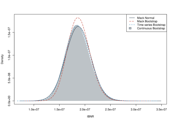
As observed in Table 2, the distribution within our framework closely resembles that of Mack with the Normal parameterized distribution and the Time Series Bootstrap. The latter offers a significant advantage: we simulate quasi-continuously (utilizing the Euler scheme), thereby eliminating negative values and resulting in a non-normal distribution.

Finally, in Figure 2, we plot the distribution of $C_{2}^{n}$ compared to the Gaussian version, using the estimated $\widehat{F}_{1}$ and $\Sigma^{2}_{1}$, as well as a Gamma distribution with the same moments.

Refer to caption
Figure 2: Estimated distributions of $C_{2}^{n}$; with $M=10^{7}$ simulations and 250 discretization steps for our Continuous model, and with parameterized Normal and Gamma distribution with the first two moments. In our continuous model, $\mathbb{P}(C_{2}^{n}=0)$ is neglected.

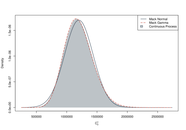
We observe that our continuous model provides a slight asymmetry which is close, in this particular case, to the one provided by a Gamma distribution.

Acknowledgments

The author acknowledges the financial support provided by the Fondation Natixis.

References

  • [1] Markus Buchwalder, Hans Bühlmann, Michael Merz, and Mario V Wüthrich. The mean square error of prediction in the chain ladder reserving method (mack and murphy revisited). ASTIN Bulletin: The Journal of the IAA, 36(2):521–542, 2006.
  • [2] Peter D England and Richard J Verrall. Predictive distributions of outstanding liabilities in general insurance. Annals of Actuarial Science, 1(2):221–270, 2006.
  • [3] William Feller et al. An introduction to probability theory and its applications. John Wiley, 2, 1971.
  • [4] Thomas Mack. Distribution-free calculation of the standard error of chain ladder reserve estimates. ASTIN Bulletin: The Journal of the IAA, 23(2):213–225, 1993.
  • [5] Sylvie Méléard. Modèles aléatoires en Ecologie et Evolution. Springer, 2016.
  • [6] Toshio Yamada and Shinzo Watanabe. On the uniqueness of solutions of stochastic differential equations. Journal of Mathematics of Kyoto University, 11(1):155–167, 1971.