Holographic drag force with translational symmetry breaking
Sara Tahery, ∗ ††∗ saratahery@htu.edu.cn Kazem Bitaghsir Fadafan † ††† bitaghsir@shahroodut.ac.ir and Sahar Mojarrad Lamanjouei ‡ ††‡ s.mojarad.sm@gmail.com
∗Institute of Particle and Nuclear physics, Henan Normal University, Xinxiang 453007, China
†,‡Faculty of Physics, Shahrood University of Technology, P.O.Box 3619995161 Shahrood, Iran
Abstract
In order to investigate how the drag force is affected by translational symmetry breaking (TSB), we utilize a holographic model in which the background metric remains translational symmetric while a graviton mass or other fields in the theory break this symmetry. We calculate analytically the drag force, considering an asymptotic AdS5 in which parameter arises from TSB. This parameter can be intuitively understood as a measure of TSB strength and we anticipate that non-zero values of it will affect the drag force. In this asymptotic AdS5 background, we will demonstrate that a decrease in results in a reduction of the drag force. Moreover, we study the diffusion constant, which falls with increasing . It will eventually be shown that at lower values of or (chemical potential), the transverse diffusion coefficient is larger than the longitudinal one, and the speed of the heavy quark has minimal impact on the ratio.
1 Introduction
AdS/CFT conjecture originally relates the type IIB string theory on space-time to the four-dimensional SYM gauge theory [1]. In a holographic description of AdS/CFT, a strongly coupled field theory at the boundary of the AdS space is mapped to the weakly coupled gravitational theory in the bulk of AdS [2]. In this conjecture the classical dynamics of a probe string in the AdS space is taken into consideration on the gravitational side.
The holographic drag force formalism is explained in [3, 4, 5] as the momentum rate flowing down to the probe string is interpreted as the drag force exerted. In the gravitational side, the presence of probe branes in the AdS bulk breaks conformal symmetry and sets the energy scales so leads to corrections in . Drag force was studied using Gubser’s proposal in the context of non-conformal models in [6, 7, 8, 9, 10].
In the context of the AdS/CFT, holographic lattices have been crafted using spatially dependent sources. These lattices demonstrate a finite DC conductivity that aligns with the results from ionic lattice calculations [11, 12]. It’s important to note that the construction isn’t limited to just explicit lattice structures. The phenomenon of momentum relaxation has been probed within the holographic domain as well. This is achieved by introducing neutral matter, serving as a vast sink where momentum from charge carriers can be transferred [13]. These charge carriers are analyzed under the probe approximation [14]. In an alternative approach, the study of momentum relaxation has been approached by adopting a theory that overtly disrupts diffeomorphism invariance within the bulk. This line of inquiry specifically involves the application of the non-linear massive gravity theory mentioned in [15] which was introduced to the holographic framework by Vegh in [16].
One may consider the Drude model in the condensed matter systems to study the motion of a probe heavy particle. It loses momentum and energy to the medium which leads to a drag phenomena. Two main mechanisms in a weakly coupled system are responsible for the drag force which are production of massless particles by bremsstrahlung and two body collisions. Study of the drag phenomena in the system helps to see which one is dominant in the system. For example radiation by a rotating heavy quark has been studied in [17] and different channels have been discussed, the extensions have been done in [18, 19]. From the condensed matter point of view, the translational symmetry in the medium breaks either by introducing impurities or periodic potentials. As a result, one expects additional new mechanisms for the energy loss in the system.
In this study, we investigate calculation of the drag force in systems where translational symmetry is not preserved. We employ holographic models that address this symmetry breaking. Although these models maintain a symmetric background metric, the symmetry is interrupted by introducing either a mass for the graviton or other fields. For example, Vegh’s model introduces mass terms for gravitons that interfere with the bulk diffeomorphisms, which correspond to translational symmetry in holography [20, 16]. Similarly, Andrade and Withers’ approach uses massless scalar fields that exhibit a linear relationship with a spatial coordinate in the field theory [21]. A model with a massless two-form field that aligns linearly with a spatial coordinate in a conformal field theory (CFT) was introduced in [22]. A comprehensive framework for translational symmetry breaking has been examined in [23], utilizing holography. This framework considers models of holographic massive gravity and manipulates translational symmetry, either explicitly or spontaneously, through a variable parameter. The dynamics of the drag force in a context of massive gravity have been previously explored in [24].
This paper is organized as follows, to use the TSB model in the drag force calculation, we briefly address it in section 2, after computation of the drag force in such system in section 3 and studying the special case of in section 4 briefly, we discuss the diffusion coefficient in section 5 and Langevin coefficients in the TSB system in section 6. Summary will be covered in section 7.
2 Translational symmetry breaking model
A general representation of the translational symmetry breaking (TSB) model we would like to work with is as follows [21],
| (1) |
where is Ricci scalar, , with AdS radius , is the field strength for a gauge field , and the massless scalar fields, . The model is written in the unit where and we will set also is the induced metric on the boundary and is the trace of the extrinsic curvature, given by where is the outward pointing unit normal to the boundary. The AdSd+1 solutions are given by,
| (2) |
where are orthogonal spatial boundary coordinates, labels the spatial directions, is an internal index that labels the scalar fields and are real arbitrary constants. The ansatz (2) leads to the solution,
| (3) |
| (4) |
where,
| (5) |
in which,
| (6) |
is proportional to the energy density of the brane and can be acquired by solving so that gives the horizon location,
| (7) |
The temperature of the black hole is given by,
| (8) |
As our current work aims to work on an asymptomatic , let’s assume in the model (1) which is written as,
| (9) |
for . Also (3), (7) and (8) are written as,
| (10) |
| (11) |
and,
| (12) |
respectively. Plugging (11) into (10) provides,
| (13) |
Demanding that gives us the constraint,
| (14) |
and imposing the null energy condition on the Ricci tensor of the metric function in (2) gives,
| (15) |
Therefore, in order to perform the calculations in the following sections, conditions (14) and (15) must be met.
In the case of the temperature vanishes. At the black hole becomes a finite entropy domain wall which interpolates between unit-radius AdSd+1 in the UV and a near horizon AdS, where the AdS2 radius, , is given by [21],
| (16) |
Note that this near horizon geometry can be obtained even when , supported by .
3 Drag force in a TSB system
We present the holographic calculation of the drag force in the presence of translational symmetry breaking using the model we previously introduced. In order to compute the drag force, consider the Nambu-Goto action as,
| (17) |
where are coordinates of the string worldsheet and is the five-dimensional Einstein metric. To describe the late-time behavior of a string attached to a quark moving in the direction in the thermal plasma with speed , we write an ansatz that ought to meet the assumption that the steady state behavior is obtained at late time. Therefore,
| (18) |
where are all terms that vanish at late time, from this point forward we ignore them. From (9) and (3) we find the Lagrangy as,
| (19) |
and from (19) the energy-momentum current is written as,
| (20) |
where ′ denotes the derivation with respect to in this case. From (20) one can obtain,
| (21) |
The right side of (21) needs to be real in order to prevent an imaginary string ansatz. Thus there should be a common root between the nominator and denominator. To apply this condition first we find the root of nominator as,
| (22) |
where is the root of (22). Following this, we arrive at,
| (23) |
By solving the equation mentioned above, we can determine that,
As previously stated, the denominator of (21) must be satisfied by the above (3) as,
| (25) |
which implies,
| (26) |
One can write from (13),
| (27) |
The current density, however, is indicated as follows,
| (28) |
As a result, the drag force is represented as,
| (29) |
where is written as (3) and is found from (27). Note that the drag force’s negative sign originates from the force vector’s direction, so in order to study we ignore the , also take the . We continue by examining the drag force’s behavior in plots. Keep in mind that we must verify constraints (14) and (15) before selecting different parameter values. Since (15) is obviously satisfied for all values, we only concentrate on (14).
(a)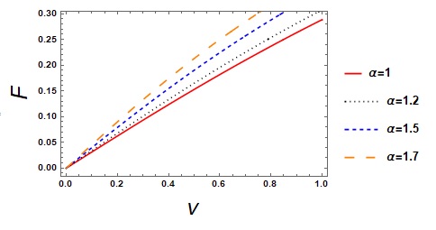 (b)
(b)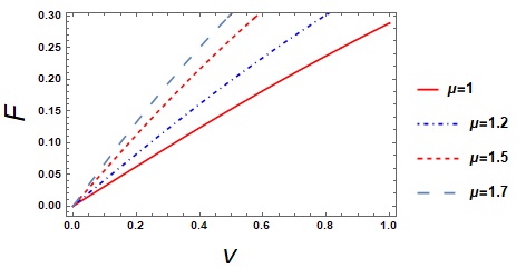
With set, figure 1 displays the drag force versus speed. Plot a) shows the effect of , with fixed. The plot demonstrates that the drag force increases in magnitude as the TSB parameter increases. Likewise with fixed plot b) illustrates the effect of , which increases the drag force. Figure 2 illustrates the drag force with respect to a) chemical potential and b) parameter for various speeds. According to both plots , the drag force is greater for larger values of .
(a)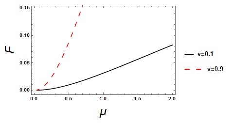 (b)
(b)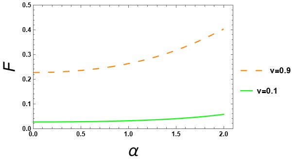
4 Drag force at zero temperature in a TSB system
That would be interesting to study motion of the heavy particle at zero temperature. One expects no energy loss in this case, however, we show that the particle experiences loosing momentum because of TSB. The drag force in extremal black holes at finite density has been studied in [25].
Examine constraint (14) at precisely , we may therefore discuss in (29) by determining different values of at some fixed .
(a)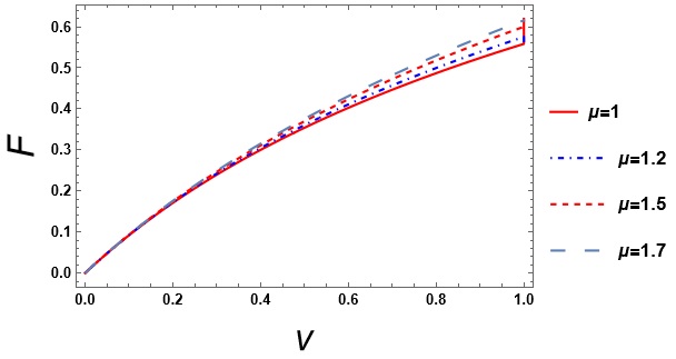 (b)
(b)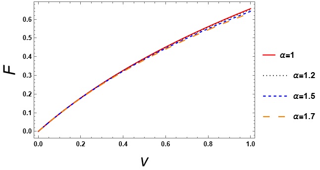
The drag force on a semi-classical string object moving at zero temperature is depicted in Figure 3. Plot (a) indicates that increasing chemical potential at zero temperature increases drag force, whereas plot (b) demonstrates that increasing has the opposite effect. We find the different effects of in a zero temperature system and a thermal medium by comparing with figure 1.
Upon holding the system’s parameters constant and varying the temperature, it is observed that the heavy particle is subjected to an increased drag force when the temperature is zero. In field theory, the observation that entropy density remains non-zero even at zero temperature indicates the existence of states to which a point particle can dissipate energy and momentum. This suggests that despite the absence of thermal energy, there are other mechanisms or degrees of freedom within the system that allow for the transfer of energy and momentum from the particle.
5 Diffusion Coefficient
The diffusion coefficient, a fundamental parameter of plasma at RHIC and LHC for heavy quarks, which is related to the temperature, the heavy quark mass and the relaxation time is defined by [3, 4],
| (30) |
where is the temperature, is the particle mass and is the damping time. It can be derived from the drag force as,
| (31) |
Therefore from (30) the diffusion coefficient is written as,
| (32) |
Like we did for the drag force in the previous section, we examine how coefficient behaves in relation to various variables in the plots that follow.
(a)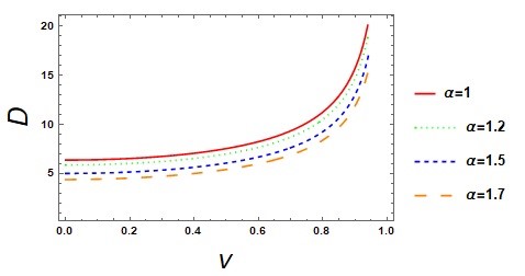 (b)
(b)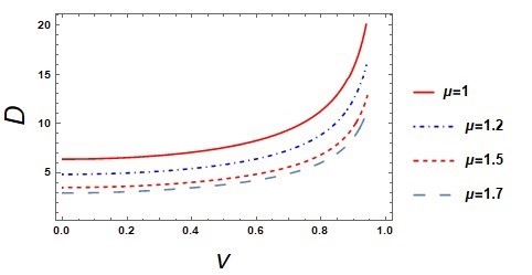
Diffusion coefficient versus speed is plotted in figure 4 for two scenarios: a) fixed and different values of , and b) fixed and different values of . In both scenarios, the diffusion coefficient decreases as the TSB parameter or chemical potential increases.
We represent the diffusion coefficient with respect to and in figure 5 for both low and high speeds, in order to examine how the diffusion coefficient varies with speed.
The diffusion coefficient rises for high speed in both scenarios, but it changes noticeably when is versus .
(a)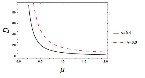 (b)
(b)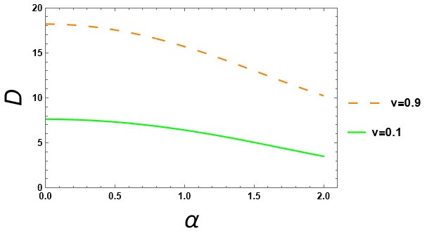
6 Fluctuations on the string in translational breaking background
Heavy quarks out of equilibrium exhibit Brownian-like motion under the influence of a stochastic force, denoted as . These dynamics produce observables that are essential to comprehending the behavior of the quark gluon plasma. One can find a thorough synopsis of the physical principles in [26]. In [27, 28, 29] an extensive research has been done on Langevin coefficients within the gauge/gravity duality. Also a universal methodology applicable to a broad spectrum of gravity theories, utilizing the membrane paradigm, was introduced in [30].
In this section, we study the relativistic Langevin coefficients in the translational symmetry background (2) using holography. Our main goal is to study these coefficients. It was argued in [31] that there is a universal inequality between transverse and longitudinal Langevin coefficients, and it only violates in an anisotropic background. We investigate its violation in the background (2). Here, we analyze the stochastic forces exerted on a quark that is in motion at a uniform speed. These forces arise due to the existence of a horizon on the string world-sheet, . The Browniaan’s motion of the quark can be modeled by the generalized Langevin equations. These equations incorporate Langevin coefficients that are proportional to the temperature of the string world-sheet, reflecting the thermal context of the motion [31]. One finds the ratio of longitudinal to transverse Langevin coefficients as,
| (33) |
(a)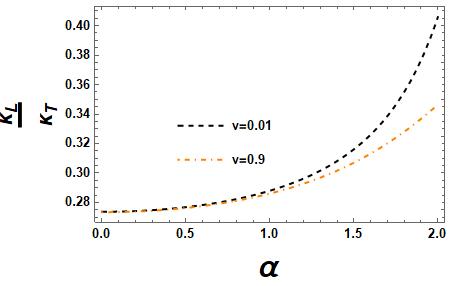 (b)
(b)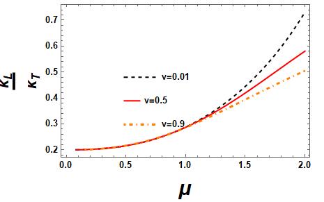
In Figure 6, we present a detailed plot illustrating the ratio as a function of the parameters and . The left-hand side of the figure is dedicated to the variation of the ratio with , while the right-hand side correlates the ratio with . It is evident from the graph that when the ratio falls below one, the longitudinal diffusion coefficient is smaller than its transverse counterpart. This observation aligns with the arguments presented in reference [30], where it was anticipated due to the violation of translational symmetry, which in turn affects the proposed bound on the ratio. The parameters and are chosen within a valid range that ensures the positivity of the temperature, a critical condition for the physical relevance of our model. The plots distinctly show that at lower values of or , the speed of the heavy quark has a negligible impact on the ratio. However, as or increase, the influence of the quark’s speed becomes significantly more pronounced. This trend suggests that the speed of the heavy quark is a crucial factor in determining the behavior of the diffusion coefficients, especially in regimes of high or . The enhanced effect at larger values points to a non-linear dependency, which could be indicative of underlying complex dynamics that merit further investigation. Such dynamics may involve intricate interactions between the quark and the medium it traverses, potentially leading to novel insights into the nature of quark-gluon plasma and the fundamental principles governing it.
7 Summary
This paper investigated the effects of translational symmetry breaking on the drag force of a system. To do so, we used a holographic model in which the parameter introduces the symmetry breaking. The effects of particle speed, chemical potential , and non-zero values of in such a system are investigated. Plots revealed that as or increase, the drag force likewise increases in magnitude, demonstrating that the strength of the TSB causes the drag force to increase. Furthermore, when plotted against or , we found that in both cases, the drag force increases with increasing particle speed, the increase becomes statistically significant when plotted against . At zero temperature, increasing chemical potential results in an increase in drag force; however, increasing has the opposite effect. Consequently, we discover that has different effects in a system running at zero temperature than it does in a thermal medium. The examination also included analysis of the diffusion coefficient. It turns out that when the TSB parameter or chemical potential increases, decreases. Furthermore, in both scenarios, the diffusion coefficient increases for high velocities; however, it manifestly varies when is versus . Finally, we discussed how the heavy quark’s speed has very little effect on the ratio at lower values of or , and how the longitudinal diffusion coefficient is smaller than the transverse one. Having said that, as or rise, the influence of the quark’s speed increases noticeably. In future works, it would be interesting to discuss the effect of TSB at high enough speed, where one can find the spatial string tension at non-zero chemical potential and the quark string configurations.
References
- [1] J. M. Maldacena, “The Large N limit of superconformal field theories and supergravity”, Adv. Theor. Math. Phys. 2, 231 (1998) [arXiv: hep-th/9711200].
- [2] E. Witten, “Anti-de Sitter space and holography”, Adv. Theor. Math. Phys. 2, 253 (1998) [arXiv: hep-th/9802150].
- [3] S. S. Gubser, “Drag force in AdS/CFT”, Phys. Rev. D 74, 126005 (2006) [arXiv: hep-th/0605182].
- [4] C. P. Herzog, A. Karch, P. Kovtun, C. Kozcaz and L. G. Yaffe, “Energy loss of a heavy quark moving through supersymmetric Yang-Mills plasma”, JHEP 07, 013 (2006) [arXiv: hep-th/0605158].
- [5] S. S. Gubser, “Comparing the drag force on heavy quarks in super-Yang-Mills theory and QCD”, Phys. Rev. D 76, 126003 (2007) [arXiv: hep-th/0611272].
- [6] E. Nakano, S. Teraguchi and W. Y. Wen, “Drag force, jet quenching, and AdS/QCD”, Phys. Rev. D 75, 085016 (2007) [arXiv: hep-ph/0608274].
- [7] P. Talavera, “Drag force in a string model dual to large-N QCD”, JHEP 01, 086 (2007) [arXiv: hep-th/0610179].
- [8] Z. q. Zhang, Z. j. Luo and D. f. Hou, “Drag force in a D-instanton background”, Nucl. Phys. A 974, 1 (2018) [arXiv: 1804.05517 [hep-th]].
- [9] Y. Xiong, X. Tang and Z. Luo, “Drag force on heavy quarks from holographic QCD”, Chin. Phys. C 43, 11, 113103 (2019) [arXiv: 1909.00928 [hep-ph]].
- [10] S. Tahery and X. Chen, “Drag force on a moving heavy quark with deformed string configuration”, Commun. Theor. Phys 74, 045201 (2022) [arXiv: 2004.12056 [hep-th]].
- [11] P. Chesler, A. Lucas, S. Sachdev, “Conformal field theories in a periodic potential: results from holography and field theory”, Phys. Rev. D 89, 026005 (2014) [arXiv: 1308.0329 [hep-th]].
- [12] S. A. Hartnoll, D. M. Hofman, “Locally critical umklapp scattering and holography”, Phys. Rev. Lett 108, 241601 (2012) [arXiv: 1201.3917 [hep-th]].
- [13] A. Karch, A. O’Bannon, “Metallic AdS/CFT ”, JHEP 09, 024 (2007) [arXiv: 0705.3870 [hep-th]].
- [14] S. A. Hartnoll, J. Polchinski, E. Silverstein, D. Tong, “Towards strange metallic holography”, JHEP 04, 120 (2010) [arXiv: 0912.1061 [hep-th]].
- [15] C. de Rham, G. Gabadadze, A. J. Tolley, “Resummation of Massive Gravity ”, Phys. Rev. Lett 106, 231101 (2011) [arXiv: 1011.1232 [hep-th]].
- [16] D. Vegh, “Holography without translational symmetry”, CERN-PH-TH/2013-357 (2013) [arXiv: 1301.0537 [hep-th]].
- [17] K. Bitaghsir Fadafan, H. Liu, K. Rajagopal, U. A. Wiedemann, “Stirring Strongly Coupled Plasma”, Eur. Phys. J. C 61, 553 (2009) [arXiv: 0809.2869 [hep-ph]].
- [18] M. Atashi, K. Bitaghsir Fadafan, “Spiraling String in Gauss-Bonnet Geometry”, Phys. Lett. B 800, 135090 (2020) [arXiv: 1906.11621 [hep-th]].
- [19] D. Hou, M. Atashi, K. Bitaghsir Fadafan and Z. q. Zhang, “Holographic energy loss of a rotating heavy quark at finite chemical potential”, Phys. Lett. B 817, 136279 (2021)
- [20] R. A. Davison, “Momentum relaxation in holographic massive gravity”, Phys. Rev. D 88, 086003 (2013) [arXiv: 1306.5792 [hep-th]].
- [21] T. Andrade, B. Withers, “A simple holographic model of momentum relaxation”, JHEP 05, 101 (2014) [arXiv: 1311.5157 [hep-th]]
- [22] S. Grozdanov and N. Poovuttikul, “Generalized global symmetries in states with dynamical defects: The case of the transverse sound in field theory and holography”, Phys. Rev. D 97, 106005 (2018) [arXiv: 1801.03199 [hep-th]].
- [23] M. Ammon, M. Baggioli, A. Jiménez-Alba, “A Unified Description of Translational Symmetry Breaking in Holography”, JHEP 09, 124 (2019) [arXiv: 1904.05785 [hep-th]].
- [24] M. Baggioli, D. K. Brattan, “Drag phenomena from holographic massive gravity”, Class. Quantum Grav 34, 1, 015008 (2017) [arXiv: 1504.07635 [hep-th]].
- [25] M. Ahmadvand, K.Bitaghsir Fadafan, “Energy loss at zero temperature from extremal black holes”, Eur. Phys. J. C 78, 10, 819 (2018) [arXiv: 1512.05290 [hep-th]].
- [26] R. Rapp and H. van Hees, “Heavy Quarks in the Quark-Gluon Plasma”, [arXiv: 0903.1096 [hep-ph]].
- [27] J. Casalderrey-Solana, D. Teaney, “Heavy Quark Diffusion in Strongly Coupled Yang Mills”, Phys. Rev. D 74, 085012 (2006) [arXiv: hep-ph/0605199].
- [28] J. de Boer, V. E. Hubeny, M. Rangamani, M. Shigemori, “Brownian motion in AdS/CFT”, JHEP 07, 094 (2009) [arXiv: 0812.5112 [hep-th]].
- [29] G. C. Giecold, E. Iancu, A.H. Mueller, “Stochastic trailing string and Langevin dynamics from AdS/CFT”, JHEP 07, 033 (2009) [arXiv: 0903.1840 [hep-th]].
- [30] D. Giataganas, H. Soltanpanahi, “Universal Properties of the Langevin Diffusion Coefficients”, Phys. Rev. D 89, 026011 (2014) [arXiv: 1310.6725 [hep-th]].
- [31] D. Giataganas and H. Soltanpanahi, “Heavy Quark Diffusion in Strongly Coupled Anisotropic Plasmas,” JHEP 06, 047 (2014) [arXiv: 1312.7474 [hep-th]].