Matter coupled to 3d Quantum Gravity: One-loop Unitarity
Abstract
We expect quantum field theories for matter to acquire intricate corrections due to their coupling to quantum fluctuations of the gravitational field. This can be precisely worked out in 3d quantum gravity: after integrating out quantum gravity, matter fields are effectively described as noncommutative quantum field theories, with quantum-deformed Lorentz symmetries. An open question remains: Are such theories unitary or not? On the one hand, since these are effective field theories obtained after integrating out high energy degrees of freedom, we may expect the loss of unitarity. On the other hand, as rigorously defined field theories built with Lorentz symmetries and standing on their own, we naturally expect the conservation of unitarity. In an effort to settle this issue, we explicitly check unitarity for a scalar field at one-loop level in both Euclidean and Lorentzian space-time signatures. We find that unitarity requires adding an extra-term to the propagator of the noncommutative theory, corresponding to a massless mode and given by a representation with vanishing Plancherel measure, thus usually ignored in spinfoam path integrals for quantum gravity. This indicates that the inclusion of matter in spinfoam models, and more generally in quantum gravity, might be more subtle than previously thought.
Introduction
Three-dimensional gravity has the crucial property to be an integral system, making it exactly soluble Witten:1988hc . More precisely, it is a topological theory, with no local degree of freedom (i.e. no graviton or gravitational waves) but only global freedom degrees coming from the manifold’s boundaries and topology. The direct consequence is that the theory can be explicitly and exactly quantized. There are several paths to this 3d quantum gravity, which together form a consistent picture of a topological quantum field theory. Nevertheless, despite being simpler than gravity in four dimensions or higher, 3d quantum gravity is clearly non-trivial and many aspects of the theory still remain to be explored. A specially relevant corner is the coupling of quantum matter to quantum gravity. Being exactly quantizable makes 3d quantum gravity the perfect toy model to gain insight on this key question of quantum gravity.
One path to 3d quantum gravity is the spinfoam quantization of 3d gravity (see Perez_2003 ; doná2010introductory ; livine2024spinfoam for introductional reviews of the spinfoam formalism) written as a gauge theory in its first order formulation à la Cartan, in terms of vierbein and Lorentz connection. It realizes a direct quantization of the theory as a topological path integral over discrete 3d geometries, leading to the Ponzano-Regge state-sum ponzano1968semiclassical , when the cosmological constant vanishes, and to the Turaev-Viro invariant Turaev:1992hq ; Turaev:2010pp , which extends it to a non-vanishing cosmological constant. It provides a regular discrete picture of the quantum space-time at the Planck scale, defining covariant transition amplitudes for the spin network states of 3d loop quantum gravity Rovelli:1993kc . It is explicitly related to the Chern-Simons quantization, both at the path integral level Freidel:2004nb or at the Hamiltonian level Noui:2004iy ; Bonzom:2014bua ; Dupuis:2019yds , and ’t Hooft polygonal quantization Kadar:2004im . Moreover its semi-classical regime is understood as quantum Regge calculus Regge:2000wu .
Of particular interest is the coupling of matter field to spinfoam path integrals. Indeed, it was shown that starting with the coupled system of matter fields and 3d quantum gravity, then integrating over the gravitational degrees of freedom leads to an effective noncommutative quantum field theory (NCQFT) for matter Freidel:2005me .The noncommutativity is controlled by the deformation parameter , identified as the 3d Planck mass (or inverse Planck length) in standard quantum field theory (QFT) conventions with and . The noncommutativity effectively deforms the Lorentz group and Poincaré symmetry, so that becomes a universal scale invariant under change of observers. Deformation of the symmetries, braiding and noncommutative star-products Dupuis_2012 ; Galluccio_2008 are well-understood mathematically. However, several questions still need to be explored and addressed, such as the fate of renormalizability, implementation of Yang-Mills gauge symmetries, causality and unitarity.
Indeed, unitarity is an essential property of QFTs, reflecting the probability flow and the conservation of information. A consistent quantum field theory should a priori be unitary. A non-unitary QFT does not seem fundamental or physically-relevant. Unfortunately, the investigation of unitarity in noncommutative geometry has been rather limited up to now. We point out two studies, Gomis:2000zz and Imai:2000kq ; Sasai:2009jm , performing a one-loop analysis using Cutksoky cutting rules. The first work studies the Moyal space, and shows that unitarity is maintained only if noncommutativity does not affect time. The second line of work studies a scalar field living in the same 3d noncommutative geometry as arising from 3d spinfoam models, that is a three-dimensional noncommutative Lie algebraic spacetime whose coordinate satisfy commutator relations, . Using group momentum space based on the group , the authors of Imai:2000kq find that the Cutkosky rule is satisfied if and only if the physical mass is less than (corresponding to a bare mass . Here, we wish to push this analysis further and investigate in more details the fate of unitarity for this noncommutative space-time , especially using the group instead of , with the goal of establishing (or disproving) the unitarity of effective NCQFTs for matter fields coupled to 3d quantum gravity as derived from the path integral formalism of Freidel:2005me .
More precisely, the Ponzano-Regge state-sum realizes a well-defined path integral of 3d gravity with vanishing cosmological constant, formulated in terms of a triad 1-form and a Lorentz connection . The action is:
| (1) |
Without particles, space-time remains flat, , and torsion-free, . Mass and momentum create curvature, while spin is a source of torsion, so that particles arise as topological defects, creating conical singularities Deser:1983tn ; tHooft:1993jwb ; tHooft:1996ziz . At the quantum level, the original model first developed in 1968 by Ponzano and Regge ponzano1968semiclassical , was revisited in the 2000’s the context of spinfoams. It was provided with a suitable gauge fixing procedure to make it finite and well-defined Freidel:2004vi ; Barrett:2008wh ; Bonzom:2012mb , leading to the proof of its equivalence with the Ray-Singer analytical torsion and Reidemeister torsion Barrett:2008wh ; Bonzom:2010zh ; Bonzom:2011br . Observables and matter insertion were consistently included as would-be gauge degrees of freedom Freidel:2004vi ; Freidel:2005bb ; Barrett:2011qe .
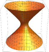
In a nutshell, the Ponzano-Regge model defines 3d quantum gravity amplitudes associated to dressed triangulations. In Euclidean signature (+,+,+), considering a finite 3d triangulation (of arbitrary topology), made of tetrahedra glued together through their triangles, we dress its edges with half-integers , which gives their quantized lengths in Planck length unit, . Each half-integer is thought as a spin, i.e. the label of the irreducible representation of the Lie group of dimension . The dressing of the triangulation with algebraic data from the representation theory of allows to dress each tetrahedron with the 6j recoupling symbol involving the spins attached to its six edges, as illustrated on fig.1. This leads to the Ponzano-Regge state-sum, or partition function, for a triangulation:
| (2) |
involving products of local amplitudes associated to each edge, each triangle and each tetrrahedron. Due to the Biedenharn-Elliott identity satisfied by the 6j-symbols, this sum does not depend on the details of the triangulation, but only on its overall topology, making it a topological invariant. The state-sum can be restricted to integer spins, i.e. representations of , with affecting its topological invariance. This restriction drops all the odd sign factors from the formula above. The extension of non-vanishing cosmological constat is achieved by considering the -deformed quantum group , as realized by the Turaev-Viro model Turaev:1992hq (see also the recent works Dupuis:2013haa ; Dupuis:2014fya ; Bonzom:2022bpv ). The extension of the model to Lorentzian signature (-++) was later developed in Barrett_1994 ; Freidel:2000uq ; Davids_2000 ; davids2001state , by dressing 3d triangulations with representations instead of . This leads to a discrete spectrum of time-like intervals and a continuous spectrum of space-like distances Freidel:2002hx .
The insertion of matter as topological defects in the Ponzano-Regge model was realized in Freidel:2005bb ; Freidel:2005me , by drawing the Feynman diagrams directly on the triangulation. First, in 3d gravity, mass is a source of curvature, while spin is a source of torsion. Putting spin aside, a point-like particle with mass creates a conical curvature. The mass is given by the angle deficit of the defect, while the particle momentum is measured by the holonomy around the defact. Second, one must distinguish the bare mass from the physical -or renormalized- mass, which fully takes into account gravitational effects. The bare mass is directly given by the defect angle in Planck mass unit, while the physical mass is given by the sine of the angle:
| (3) |
which automatically satisfies the Planck mass bound .
For scalar fields, we draw Feynman diagrams on the triangulated space-time by inserting off-shell particles along the triangulation edges. So, drawing a Feynmann diagram on a subgraph in the triangulation, with masse angles on the graph edges gives the following Ponzano-Regge amplitude,
| (4) |
where corresponds the insertion of Feynman propagator. Fields with spins can also be taken into account Freidel:2004vi ; Freidel:2005bb . Actually, this formula was previously only written for representations, in Freidel:2005me ; Livine:2008sw . So we will work out the general case, of representations, in the present work, and notice ambiguities in the definition of the deformed Feynman propagator, which were missed by earlier works.
These quantum gravity amplitudes with (off-shell) matter insertions can be summed exactly and yield Feynman diagrams of a braided NCQFT, where the 3d Poincaré symmetry is upgraded to the Drinfeld double of . The effective action of the noncommutative scalar field is defined on the non-commutative space-time , which is the space equipped with a non-trivial -product rendering the coordinates non-commutative with commutation relations (or in the Lorentzian case). The momentum space is then the Lie group (or in Lorentzian signature). This makes possible to write the NCQFT action as a group field theory (see Oriti:2009wn for a review of the GFT framework) and actually derive it directly from Boulatov’s group field theory for the Ponzano-Regge model Fairbairn_2007 (see Boulatov:1992vp for Boulatov’s group field theory paper).
The question of unitarity of this NCQFT was mentioned in Freidel:2005me 18 years ago and briefly investigated in Sasai:2009jm , and, despite its importance, has been shelved until now. In fact, it is a fundamental question for noncommutative quantum field theory and quantum gravity. Indeed, we expect two different results, depending on how we look at the theory. On the one hand, if we consider this model as an effective field theory, derived from a more fundamental theory after integrating out degrees of freedom, unitarity should naturally fail as soon as we reach high enough energy to excite the integrated-out modes. On the other hand, if we view those NCQFTs as legitimate well-defined and mathematically rigorous field theories directly built from scratch on the non-commutative space-time , is is natural to expect unitarity, the existence of a probability current and conservation of information.
In the present work, we check the unitary at the one-loop level using the Cutkosky rule in both Euclidean and Lorentzian cases. We find that Lorentzian and Euclidean versions of the Cutkosky rule are valid for and only for small mass. Furthermore, they are valid for and for all masses, if we add an extra term to the Feynman propagator. This extra term is a 0-mode, actually corresponding to a infinite-dimensional representation of in the Euclidean theory and corresponding to a representation of on the light cone, with vanishing Plancherel measure, and usually refered to as the limit of discrete series knapp2001representation . The paper is organized as follows. The first section presents the noncommutative theory for matter coupled to 3d quantum gravity. The second section reviews the Cutkosky rule for standard QFT in commutative space-time. We take special care to clearly derive the counterpart in Euclidean space-time signature of the optical theorem at one-loop. We then move on to the investigation of the Euclidean noncommutative theory based on and . We describe the different propagators and then compute explicitly the on-shell and off-shell one-loop amplitudes to check the validity of the Cutkosky rule. We underline the key differences between and its double cover. We then tackle the heart of our work and analyze the Lorentzian theory, for which we also derive propagators and explicitly compute the one-loop amplitudes for the and momentum spaces. Finally, we discuss the implication of our results for the unitarity of the NCQFTs and underline interesting lines of future investigation.
I Noncommutative scalar field theory on
We are interesting in a class of noncommutative field theory built from curved momentum spaces. Assuming that the momentum space has the structure of a semi-simple Lie group , we consider the following scalar field actions:
| (5) |
where we integrate using the Haar measure over the Lie group. The kernel defines the kinetic term, while enforces the conservation of momentum in the -valent interaction term. A non-abelian group product translates into a noncommutative addition of momenta. The noncommutativity of spacetime coordinates can then be derived by taking the group Fourier transform of this action (see e.g. Freidel:2005ec ; majid2000foundations ; Girelli:2022foc ).
Here, in the context of 3d quantum gravity, we are interested in the case that the Lie group is or for an Euclideanspace-time signature and or for the Lorentzian theory. Then the kinetic kernel is taken of the form . We will restrict to the cubic self-interaction for the sake of simplicity, in which case the action reads
| (6) |
The momentum is defined as the projection on the group element on the Euclidean or Lorentzian Pauli matrices depending on the chosen space-time signature. More precisely,
-
•
In the Euclidean theory:
We project on the Pauli matrices , satisfying for all . In the fundamental two-dimensional representation, a group element decomposes onto the Pauli matrices and the identity as , with the half-angle of rotation and the rotation axis. Obviously this is a redundant parametrization, with the identification of the group elements and (,), so we can safely restrict to angles . The projection is simply defined as:(7) This is a well-defined momentum map, since it is invariant under the exchange . It is crucial to notice that the map is onto but not bijective. Indeed changing the sign of the cosine, i.e. mapping the angle , does not change the momentum:
(8) This two-fold degeneracy can be lifted by using the group instead of . Indeed, a group element is defined by the equivalence relation , which corresponds to in the angle-axis parametrization. We can therefore choose group elements as corresponding to angles , thus with positive sine and cosine. Then a 3-vector , norm-bounded by , corresponds to a unique group element with (thus pointing in the same direction) and .
-
•
In the Lorentzian theory:
We work with space-time signature and we use the Pauli matrices , . Group elements of are of three types. Elliptic or time-like group elements read , with and the class angle . Similarly to the Euclidean case, this parametrization is redundant and . If we want to keep a definite direction for the rotation axis , we should lift this degeneracy and restrict to angles . This allows to identify elements with as positive time-like, and those with as negative time-like. Hyperbolic or space-like group elements are , with . Note that the sign can not be absorbed by a modification of or . We have the same degeneracy as for elliptic group elements with , which is simply lifted by restricting to positive boost parameters . Finally, null group elements are , with .Momentum is defined, as in the Euclidean case, by projecting group elements on the Pauli matrices,
(9) where only elliptic group elements have bounded momenta.
The map is once again onto but not bijective. This can be lifted by using the subgroup , defined by the equivalence relation . This amounts to restricting the class angle of elliptic elements , dropping the sign in front of hyperbolic and null elements. This makes the momentum map bijective.
At this stage, in both Euclidean and Lorenztian signatures, we clearly see the difference between the bare mass and the renormalized mass . The bare mass keeps increasing as the defect angle grows from 0 to , while the renormalized mass is not in one-to-one correspondance with the angle: it increases in the range , reaches its maximum at then decreases. We therefore expect the large mass sector to exhibit large (quantum) gravitational effects. We will indeed see that the field theories based on or momentum space will fail to be unitary due to this large mass sector. In order to correct this bad feature, one has to move to the double-covers or , and introduce a Feynman propagator that distinguishes the angles and . So instead of merely using , we will also simply use to define the kinematics of the NCQFT. At the end of the day, this will fix the unitarity (at least, at the one-loop level).
Using this momentum , one can perform a change of variables, from group elements to usual vectors , and write our field theory (6) in term of standard momenta variables Freidel:2005me :
where the non-commutative addition of momenta is inherited from the non-abelian group multiplication,
| (11) |
The measure factor is inherited from the Haar measure. It reads explicitly for or :
| (12) |
Remember that momenta are always bounded, , for , while this bound also holds for time-like vectors in (i.e. elliptic group elements) for . For the or groups, the change of variables is not bijective, so we need to sum over an extra sign when writing the theory in terms of vector momentum. Details on the resulting measures can be found in the appendix A.
In the limit of an infinite Planck mass, when the deformation parameter is sent to infinity, , we recover the standard commutative momentum space equipped with the trivial addition of momenta,
| (13) |
One can then compute the quantum gravity corrections to standard quantum field theory order by order in , as shown in Freidel:2005bb . This formalism clarifies how the Planck mass encodes the quantum gravity fluctuations and contributions to the effective field theory.
It is possible to define a group Fourier transform to go from the action (6) in terms of group variables, or the action (I) in terms of noncommutative momenta, to an action written in coordinate space Freidel:2005me ; Freidel:2005ec . The key is that the group product, or equivalently the noncommutative addition of momenta, equips functions over the 3d coordinates a non-trivial -product, which is simply defined in terms of plane-wave multiplication on :
| (14) |
This -product leads to a non-commutativity of the space-time coordinates,
| (15) |
This allows to write the field action in coordinate space Freidel:2005bb :
| (16) |
For more details on this -product, the interested reader can check Freidel:2005ec ; Livine:2008sw ; Livine:2008hz ; Dupuis_2012 . The aim of the present work is to study the unitarity of these noncommutative field theories in both Euclidean and Lorentzian signatures.
II One-loop integrals and cut rule
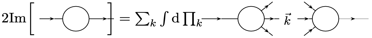
In this section, we compute the leading one-loop correction to the field propagator for the standard undeformed Euclidean and Lorentzian 3d theories. Unlike the 4d theory, where one-loop amplitudes have logarithmic divergences, we have finite expressions in 3d. We can thus check unitarity with the Cutkosky rule at one loop without any regularization. In a Lorentzian space-time, for time-like external momentum, this rule states that the imaginary part of the off-shell one-loop amplitude is equal to its on-shell counterpart, as illustrated on figure 2. If we denote the amplitude for Lorentzian off-shell one loop, with external momentum , and the Lorentzian on-shell one loop, they satisfy the following relation:
| (17) |
We review the computation these amplitudes below and check this relation.
We also derive a Euclidean version of this cut rule, relating the Euclidean off-shell and on-shell one-loop amplitudes. We will then be ready to check if the same Euclidean and Lorentzian rules are also satisfied by the non-commutative quantum field theory at one-loop.
II.1 Field theory in Euclidean signature
The Feynman propagator for mass in Euclidean signature is the solution of the Klein-Gordon equation with Dirac- source . It is given by the Fourier transform of , where a regulator,
| (18) |
which is straightforward to integrate,
| (19) |
The one-loop diagram with two momentum insertions gives the leading order correction to the field propagator. Its amplitude is an integral over the momentum running around the loop:
| (20) |
which can be computed exactly, yielding:
| (21) |
One notices the apparition of a non-vanishing imaginary part above the two-particle threshold . Let us compare this exact one-loop diagram to the corresponding on-shell integral:
| (22) |
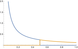
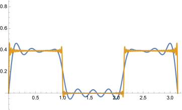
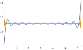
We find that the imaginary part of the one-loop diagram is equal to its on-shell counterpart up to an awkward inversion of the mass-momentum threshold condition . This means that, eventhough this Euclidean theory is clearly not unitary, we nevertheless have the following relation between the imaginary part of the off-shell and on-shell one-loop integrals, as plotted on fig.3:
| (23) |
with either functions vanishing when the other does not: vanishes for , while vanishes for . In some sense, one could say that these two functions complete each other. This is our Euclidean counterpart of the Lorentzian optical theorem. We will seek to check whether a similar relation holds for the Euclidean noncommutative field theory.
II.2 Field theory in Lorentzian signature
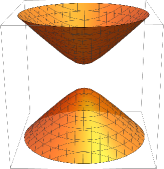
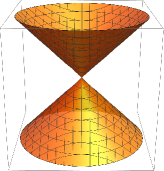
Let us now check how the one-loop calculation works in the more standard Lorentzian field theory, with metric signature . There are three types of momenta, as illustrated on fig.4. There are time-like vectors characterized by a positive norm, . They live in one of the two sheet hyperboloids of the Lorentzian space. We distinguished positive time-like vectors, with positive time component , living in the upper hyperboloid from negative time-like vectors, with , living in the lower hyperboloid . The second one is space-like vectors, which have a negative norm, i.e., , and they live in the one-sheet hyperboloid.
The Feynman propagator for mass is the solution of the Klein-Gordon equation with Dirac- source. It is given in momentum space by , where the momentum norm is . We write the off-shell one-loop using Feynman’s parametrization:
| (24) |
It is possible to compute exactly those integrals, taking special care of properly distinguishing time-like and space-like momenta. The integral in can be computed by a Wick rotation and gives:
| (25) |
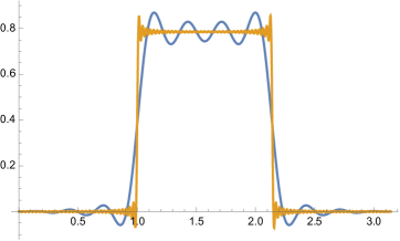
Let us first consider an external time-like momentum, with . For , the interior of the square root is always positive, and we recognize the primitive of . For , we have a branch cut, producing an extra imaginary contribution. Overall, one gets:
| (26) |
On the other hand, the computation of the on-shell one-loop amplitude amounts to integrating -functions:
| (27) |
As expected, we recover the optical theorem at the one-loop level for time-like elements,
| (28) |
Interestingly, the off-shell one-loop integrals are the same in Euclidean and Lorentzian theories, whereas the on-shell one-loop integrals have inverse conditions on . We expect to find a similar behavior for the noncommutative theories.
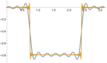
For space-like external momentum, , the off-shell integrals do not have any imaginary part,
| (29) |
while the on-shell integral gives:
| (30) |
The Cutkosky rule unsurprisingly fails in this case. This is to be expected, since space-like momentum us not a physical state, so that one can not expect the optical theorem to hold. Moreover, there is no obvious counterpart of the cut rule for this configuration.
III NCQFT Unitarity and Feynman Propagators: Euclidean case
In this section, we detail the structure of the one-loop integral for the noncommutative quantum field theory on the Euclidean . In particular, we compute both Hadamard and Feynman propagators. We first tackle the momentum space, then derive work out the case of the momentum space. As pointed out earlier, the field theory allows for a one-to-one map between group elements and momenta. However, since the Lie group is obtained by a identification, we do expect an impact of quotienting by this discrete group. We will explain how it affects unitarity and actually ruins it at high momenta. On the other hand, the field theory has a degenerate two-to-one map between group elements and momenta, so one needs to investigate and understand the physical impact of this degeneracy.
Let us make an important remark. In noncommutative quantum field theory, at the one-loop level, one should consider a supplementary non-planar Feynman diagram (i.e. with lines crossing over each other), on top of the standard one-loop diagram, as illustrated on the second diagram on fig.5).
Such diagrams are actually at the origin of UV/IR mixing in NCQFTs and do not have any classical equivalent Hersent:2020lsr It has nevertheless been shown that the case of the non-commutative space-time has some simplifying propreties. Indeed, due to the braiding of the NCQFT as shown in Freidel:2005bb ; Sasai:2007me , such non-planar diagrams are equivalent to the standard planar one-loop diagram Sasai:2009jm . It is therefore enough to study the cutting rule for this planar one-loop Feynman diagram.
III.1 Feynman and Hadamard propagators on
Let us start with the noncommutative field theory based on the momentum space. The case will be dealt with afterwards, and can be found at the end of this section.
Massive particles are encoded in 3D gravity as topological defects parameterized by an angle , leading a renormalized mass Deser:1983tn ; Matschull:1997du . This is this renormalized mass that enters the effective noncommutative field theory action (6). The Feynman propagator can be read directly from the kinetic term of this action. In momentum space, it is given by Freidel:2005bb :
| (31) |
Its Fourier transform gives the Feynman propagator in coordinate space,
| (32) |
This propagator actually satisfies the Klein-Gordon equation with mass M and a -distribution source, which is the noncommutative counterpart of the standard -distribution. It is the most localized distribution in coordinate space in the noncommutative ,
| (33) |
normalized to , where is the standard Bessel function of the first kind. Using this insight, it is possible to write the Feynman propagator as a convolution product in the radial coordinate ,
The integral on the right vanishes as goes to infinity, and the leading order of the deformed Feynman propagator at large distances is given by the standard Feynman propagator, up to a numerical factor:
| (35) |
The integral term in the expression of the NCQFT propagator thus describes the noncommutative correction to the standard QFT propagator. Note that it only affects its real part.
On the other hand, at a short distances, when , the behavior of the propagator is strongly affected by the space-time noncommutativity, which fully regularizes it. Indeed, the deformed Feynman propagator is finite at unlike its standard counterpart:
| (36) |
Another insightful expression of the Feynman propagator is given by its character expansion. Indeed, in momentum space, it is actually a (central) function over and can thus be expanded over the characters of its irreducible representation, that is, in short, as a series over spins. More precisely, an orthonormal basis of square-integrable functions on the Lie group , invariant under conjugation, is given by the characters for integer spins . The character is the trace of the group elements in the spin- representation,
| (37) |
where is the dimension of the representation of spin . We expand the Feynman propagator in this basis:
| (38) |
where the coefficient can be computed as a contour integral111 We start from the explicit expressions of the Feynman propagator and characters as central functions on , and . Then, since the Haar measure on for central functions can be simplified to for running from 0 to , we write the coefficients of the spin expansion of the Feynman propagator as contour integrals in the complex plane, where and is the unit cercle in . The denominator can be expanded and we find poles around : We can then evaluate the integral using the residue formula. Since , only the poles in contribute and we obtain the announced decomposition. ,
| (39) |
These coefficients are the quantized equivalent of the coordinate expression of the Feynman propagator. Indeed, as explained for example in Freidel:2005ec , the spin is best interpreted as the quantized radial coordinate in the context of 3d quantum gravity and noncommutative coordinate operators. Comparing to the previous expression (III.1) for , we indeed see that the expression for is simpler and does not involve any extra term. So, in some sense, one has traded the integral correction in for a discrete length spectrum in , both reflecting the effect of noncommutativity.
Following the usual treatment of propagators in QFT, we define the Hadamard propagator from the imaginary part of the Feynman propagator:
| (40) |
where we recognize the Dirac distribution on fixing the class angle of the group element to the mass angle ,
| (41) |
where the distribution is the Dirac distribution fixing the class angle in :
| (42) |
As expected, the Hadamard propagator encodes the mass-shell condition on , which is the noncommutative equivalent of in standard QFT. Let us underline the appropriate identification between the class angles and , reflecting the identification of group elements . This identification restrict the sum from half-integers to integers, as expected. More details on distributions on versus can be found in appendix B.
We are now ready to tackle the case of a momentum space and the corresponding Feynman propagator. The main obstacle of working on is that the momentum map is not bijective but two-to-one, and thus there is no proper Fourier transform between and . Working on actually allows to bypass this issue, by identifying the group elements . From this point of view, working on instead of means to be able to distinguish from . Some solutions to define an appropriate group Fourier transform have been proposed, e.g. lifting the 3d integrals to 4d in Freidel:2005ec , or introducing an extra measure factor in Livine:2008sw , or using the Schwinger parametrization in terms of spinorial variables Dupuis_2012 . As we are interested here in the QFT propagators, the most straightforward method to lift all decomposition over integer spins to series over all half-integer spins.
Then, simply extending the previous series to half-integers, one can guess an appropriate Feynamn propagator on the momentum space:
| (43) |
Taking its imaginary part gives the corresponding Hadamard propagator:
| (44) |
where we recover the expected mass-shell condition, fixing the class angle of the group element in . As wanted, we have lifted the identification the identification , or equivalently . The new Feynman propagator amounts to modifying the kinetic term of our original NCQFT,
| (45) |
from the original theory written in Freidel:2005bb ; Freidel:2005me ,
| (46) |
to a new version based on the character of spin instead,
| (47) |
This propagator version was actually derived in previous work from 3d quantum gravity in the group field theory formalism Fairbairn_2007 and interpreted as filling the discrete Ponzano-Regge path integral with spin- defects Livine:2011yb ; BenGeloun:2018eoe .
However we will go further than this propagator ansatz and add a extra term. We will see later in section III.3 that this new term is necessary to ensure unitarity at one-loop. Explicitly, we introduce an enhanced Feynman propagator:
| (48) |
where we have added a term interpretable as the -representation with vanishing . Actually, it is an infinite-dimensional representation with Casimir , thus corresponding to a negative spin . Its character would be and diverges at the identity , . Nevertheless, this divergence goes away with the Haar measure and only leads to a constant offset of of the Feynman propagator after a Fourier transform. This new 0-mode term does not affect the relation between the Feynman and Hadamard propagators,
| (49) |
so it is a legimitate ansatz for a Feynman propagator. Finally, in the commutative limit where the deformation parameter is sent to infinity, , this extra term vanishes, and we recover as wanted the standard Feynman propagator of the undeformed QFT. Nevertheless, the physical interpretation of this extra 0-mode is not quite clear, it translates, after inversion, into a more complicated kinetic term in the field theory action, and we will discuss its role more in section Conclusion and Outlook.
III.2 One-loop unitary: Feyman propagator
Now that the propagators are well-defined for this Euclidean field theory, let us move on to the computation of the one-loop integrals as illustrated on figure 6 with on-shell and off-shell propagators. This will allow us to check the validity (or not) of the Cutkosky’s cut rules for the non-commutative field theory with momenta.
Let us fix the mass angle . Indeed masses and are equivalent so we can safely restrict from the interval to . Let us then start by analyzing the one-loop integral with on-shell propagators. Its expansion on characters reads:
| (50) |
This expression can be explicitly computed either from the sum over spins or the integral over the group. Details are given in appendix B. We must distinguish different cases according to the value of the mass angle , as shown on the plots in figure 7.

For a mass angle , we get:
| (51) |
while, for a mass angle , we get a extra contribution:
| (52) |
Let us keep in mind that these expressions are invariant under . Comparing with standard undeformed field theory, the sector corresponds to the sector , while there is no classical counterpart to the “IR-UV” identification due to working with momenta.
We now compute the off-shell one-loop with incoming momentum , internal momentum and mass angle , as illustrated on fig.6.
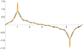
Using the character expansion of the Feynman propagator, this one-loop integral with off-shell propagators read:
| (53) | |||||
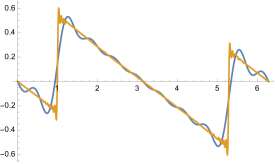
We notice the same pre-factor in as for the on-shell integral. We plot the real and imaginary parts of the series in figures 8 and 9, in order to visualize the various cases. The series can be summed exactly and yields for :
| (54) |
For a mass angle in the upper half-range , we get:
| (55) |
where the only notable change is the switch of sign in the imaginary part for higher values of the incoming momentum . This is simply due to a sign switch of the expression in the logarithm.
At the end of the day, comparing the off-shell and on-shell integrals, we see that the Euclidean version of the Cutkosky cut rule is valid in the noncommutative field theory at small masses, with (corresponding to where is the Planck mass)
| (56) |
with the imaginary part of the off-shell integral vanishing for momenta and , while the on-shell integral vanishes for all other values of the momentum . On the other hand, once the mass is large enough, for , this cut rule is violated and unitarity fails, due to the new non-vanishing term in the on-shell amplitudes for momentum . In the following section, we will see how one can fix this problem by properly working with a momentum space instead of .
III.3 One-loop unitary: Feyman propagator
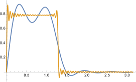
Let us now look into the one-loop amplitudes based on the momentum space. The on-shell diagram uses the Hadamard propagator, given by the distribution fixing the class angle in ,
| (57) |
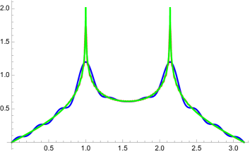
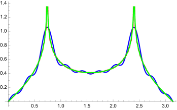
where we underline that the main difference with the case is that we now sum over all half-integer spins . This series can be summed exactly. This gives us for and :
| (58) |
where we see the expected threshold at , as shown on figure.10, with a step drop from the constant value down to 0.
We can compute this series for higher angles . This gives an inverted behavior with a second threshold at , as illustrated on figure 10. Let us nevertheless point out that we can restrict ourselves to to avoid redundacy in our angle-axis parametrization of group elements, and thus discard higher values of the angle as physically irrelevant.
Finally, for higher mass angle , the profile stays the same but the two thresholds at and now plays inverse roles, as shown on figure 11.

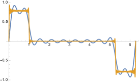
The computation of the off-shell Feynman diagram is more subtle due to the possible ambiguity in the definition of the Feynman propagator, as discussed earlier in section III.1. Indeed, it is possible to change the real part of the Feynman propagator while respecting the constraint that its imaginary part reamins the Hadamard propagator giving the mass-shell condition. Let us first try the “naïve” ansatz (43), given explicitly by
then the one-loop integral yields,
| (59) |
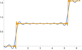
This series can be summed exactly222 can be computed by integrating over . This gives a term in which can be re-written as: . We plot its real and imagniary parts in figure 12. However one find that it violates the Euclidean version of the optical theorem:
| (60) |
with the expected term on the right hand side, corresponding to the term in our Euclidean version of the cut rule in standard commutative QFT, but now with an extra anomalous term , as illustrated by the plots in figure 13.
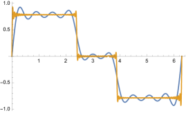
Making this theory unitary thus require to kill this anomaly. As we announced in the previous section, we have identified an appropriate modification of the Feynman propagator that compensate this anomalous term, by introducing an extra 0-mode term as given in (48), which we remind here:
This new term has a pole at , i.e. on the vanishing momentum . This creates a resonance at zero mass, thus we identify as an extra “0-mode”. This modification of the the Feynman propagator compensates exactly the anomaly in the one-loop integral,
| (61) |
The real part of this one-loop Feynman amplitude is given by a log, while the imaginary part satisfies the Euclidean version of the optical theorem; that is, explicitly for all :
| (62) |
Thus, with this corrected Feynman propagator, the NCQFT verifies the Euclidean version of the Cutkosky cut rule at one-loop. And, unlike the case, there is no surprise when the mass angle goes above .We have thus cured the awkward feature at high mass of the propagator, by avoiding the somewhat unphysical identification between momenta and . This gives hope to get a truly unitary theory in Lorentzian signature, at least at the one-loop level, by similarly correcting the Feynman propagator . We show in the next section that it is indeed the case.
IV NCQFT Unitarity and Feynman Propagators: Lorentzian theory
In this part, we move to the Lorentzian quantum field theory, based on momenta living in the groups or its double cover . This NCQFT is meant to drive the propagation of quantum fields coupled to 3d quantum gravity in Lorentzian signature, described by the Lorentzian version of the Ponzano Regge state-sum Freidel:2000uq ; Davids:2000kz . We define the Hadamard and Feynman propagators encoding the mass-shell conditions and off-shell correlations of the quantum field in non-commutative space-time. We then compute the one-loop integrals and show that the NCQFT based on with a suitably 0-mode corrected Feynman propagator is indeed unitary (at the one-loop level).
IV.1 Lorentzian Feynman and Hadamard propagators
In order to generalize our approach from the Euclidean case to the Lorentzian theory, we face four potential issues:
-
•
properly deal with the non-compactness of the Lorentz groups, and , with infinite-dimensional unitary representations;
-
•
carefully deal with the difference between time-like and space-like momenta, corresponding to elliptic and hyperboloic group elements having compact or non-compact conjugation orbits;
-
•
keep in mind the difference between and , which ended up playing a crucial role in the Euclidean field theory;
-
•
understand the possible admissible corrections to the Feynman propagator, and use this ambiguity to identify the one(s) compatible with one-loop unitarity.
Indeed, the foremost difference between the Euclidean and Lorenztian cases, is that the Lorentz groupes and are non-compact compared to their Euclidean counterparts, and . The direct consequence is that their unitary representations are automatically infinite-dimensional. This algebraic fact has a direct analytical consequence since, following the Plancherel formula, central functions and distributions are to be expanded on the characters of these unitary representations.
The unitary representations of involved in the Plancherel decomposition are called the principal series Bargmann:1946me . There are of two types (see e.g. Davids:2000kz ; Kitaev:2017hnr for more details):
-
•
The principal continuous series are parametrized by a real number and a parity . Their Hilbert space is spanned by states with if or if . The eigenvalue of the Casimir is while the number diagonalizes . The character of the representation does not depend on the parity , its vanishes on elliptic group elements whiile it oscillates on hyperbolic group elements:
(63) where one should remember that hyperbolic group elements are conjugate either to or to , without any possibility of switch sign by conjugation, even if a group element with boost parameter is obviously conjugated to with boost parameter (but without changing the overall sign in front of the group element).
Representations of are only the ones with positive parity, .
-
•
The positive and negative discrete are parametrized by a half-integer and a sign . Their Hilbert space is spanned by states with if or if . The Casimir is given by . The character of the representation oscillates on elliptic group elements , it does not vanish on the hyperbolic group elements but admits an exponential tail:
(64) Representations of are only the ones with integer spin , which satisfy .
The Plancherel measures for and was found by Harish-Chandra Harish and give the decomposition of the -distribution in terms of the characters of the principal series of unitary representations. Let us start with . The Plancherel formula is:
| (65) |
where we write . Notice the sign switch with respect to the Euclidean case:
| (66) |
To impose the mass-shell condition, we need a distribution enforcing that the group element is elliptic and fixing its class angle to a given . This is given by:
| (67) |
The coefficients are determined by the condition that vanishes on hyperbolic group elements. In fact, one can compute the sum over spins for a group element as a geometric series:
| (68) |
Then the condition that imposes that the coefficients be the Fourier transform of this function in :
| (69) |
which, by a straightforward residue computation,333To apply residue formula, we chose a rectangle un the upper plane of length and height , along vertical segements we can easily show that the integral of vanish. It remains the two horizontal segements which give a non zero contribution to the function: (70) . In the rectangle there are two poles, and , using the residue theorem: (71) Finally thanks to L’Hôpital’s rule one gets 72 finally yields for arbitrary :
| (72) |
Then evaluating the same expression on elliptic group elements gives:
| (73) |
We can adapt all these formulas to the case. One should remember that we need to identify and , or equivalently identify the angles and . Then the Plancherel formula becomes
| (74) |
Then fixing the mass-shell amounts to fixing the angle to either or ,
| (75) |
where the coefficients are derived from the ’s:
| (76) |
This distribution vanishes on hyperbolic group elements by construction and yields the expected -distribution on :
| (77) |
The interested reader will find more details on distributions on and in appendix C.
Let us now turn to the Feynman propagator. We read it off directly from our field theory action (6) Freidel:2005bb ,
| (78) |
This propagator is the same as in Imai:2000kq ; Sasai:2009jm but with a different sign convention due to a difference of signature . A straightforward calculation gives the character decomposition of :
| (79) |
We recognize in the first term the the character expansion of the Euclidean Feynman propagator. In contrast, the second term gives the exponentially decreasing tail of the Feynman propagator for space-like intervals. This second term was missed in Freidel:2005bb .
We deduce the Hadamard propagator from the imaginary part of this Feynman propagator:
| (80) |
which gives the mass-shell condition. We thus refer to as the Hadamard propagator. The reason why this leads to and not to the mass-shell is the same as the Euclidean case. Indeed, the Feynman propagator does not distinguish the four group elements . The symmetry of the propagators under the exchange is natural and corresponds to the standard symmetry. What’s more subtle is the confusion , which does not have any counterpart in the standard commutative field theory. Similarly to what we achieved in Euclidean signature, we can lift this confusion by introducing an appropriate propagator.
Indeed, let us now define the Feynman propagator, by including odd parity representations (i.e. from the continuous series with and from the discrete series with half-integer spins), as well as including an extra 0-mode:
| (81) |
where we included an extra-mode, similarly to what we did in the Euclidean case:
| (82) |
This is an eigenvector of the Casimir with eigenvalue , thereby formally corresponding to a spin , thus the notation. It should correspond to the character of the exceptional (or mock) discrete representation, which is the limit of the principal discrete series of unitary representations of and has vanishing Plancherel measure.
The integral over the continuous series labeled by was already computed above, while the series in the spin can be resummed exactly as a geometric series for . The convergence is numerically very fast, except close to , and gives:
| (83) |
This Feynman propagator leads a Hadamard propagator which properly reflects the mass-shell condition , where the sum over both signs is due future and past orientation for the time-like momentum:
| (84) |
We show below that this propagator defines a unitary quantum theory at the one-loop level.
IV.2 Lorentzian one-loops integrals and unitarity
Now that the propagators of the Lorentzian field theory have well-defined as distributions on the Lie groups and , we can analyze the one-loop diagrams of the quantum field theory and check whether they satisfy the optical theorem or violates unitarity. We consider the one-loop diagram with incoming group element . To distinguish past and future orientations, one must restrict the angle to lay in the interval .
First, let us analyze the theory with its Feynman propagator . Due to the identification between the group elements and in the case of , we further restrict the range of the angle to . The off-shell and on-shell one-loop integrals read:
| (85) |
To compute the off-shell one-loop in the non-commutative Lorentzian theory, we look at the non-deformed field theory and notice that the Euclidean and Lorentzian off-shell one-loop amplitudes are similar and involve the same integrals. This feature is carried to the deformed theory, and we actually show that Lorentzian off-shell computation is equal to Euclidean off-shell one-loop.
Indeed, in the Euclidean case, we consider group elements, the external momentum and the momentum along the loop , and call the class angle of . The off-shell one loop then explicitly reads (see Appendix A for details):
| (86) |
where is the angle between the rotation axis of and . In the Lorentzian case, we consider group elements, the past-oriented external momentum and the loop momentum . We call the angle of the composed momentum . After making the suitable change of variables from the boost parameter between and to the rapidity of the composed momentum, the off-shell one loop reads (see appendix A for details):
| (87) | |||||
This shows that the Lorentzian expression is equal to its Euclidean counterpart, which has already been computed before. This is consistent with the standard undeformed QFT where Euclidean and Lorentzian off-shell one-loops were also equal. This yields:
| (88) |
As for the on-shell amplitude, one can integrate exactly the -distribution entering the on-shell loop diagram (see appendix C for details). For and , we get:
| (89) |
Thus for a mass angle lying in the interval , the cutting rule is satisfied. However, when the mass increases and lays in range , the on-shell one-loop integral always vanishes.
| (90) |
The cutting rule is no longer satisfied. This is the same issue that we encountered in the Euclidean theory at large mass. Thus, we can conclude that the optical theorem only applies to angles , corresponding to small masses (or bare mass ): increasing the mass fully puts in light the un-classical behavior of the on-shell one-loop amplitude. We recover exactly the result previously found Sasai:2009jm , which showed the non-unitarity of the 3d Lorentzian noncommutative scalar field theory based on the momentum space. Here, we go further that this previous work and show how to fix the unitarity of the NCQFT by using a Feynman propagator fully reflecting the structure of the momentum space.
Let us then turn to the -based theory and its Feynman propagator , involving all even and odd representations of as well as the extra 0-mode coming from the exceptional discrete representation of spin . Working with the full group, the angles can be restricted to the range in order to avoid redundancies. However, we drop the identification between and defining the subgroup, so the interval can not be reduced to , we need to take . Following what we obtained for the Eculidean theory, we expect to find a cutting rule verified for all masses .
Off-shell and on-shell loop expressions are given by:
| (91) |
The off-shell amplitude has a similar expression to its Euclidean counterpart, the off-shell one loop. Details of the computation of both on-shell and off-shell integrals can be found in appendix C. The final result, for and , reads:
| (92) |
| (93) |
Thus, using the modified Feynman propagator, we recover the Cutkosky rule for an arbitrary mass . The noncommutative field theory is therefore unitary at the one-loop level, and can be considered as a legitimate physical field theory.
Conclusion and Outlook
In this paper, we have looked into the unitarity of non-commutative quantum field theory (NCQFT) based on the space-time in both Euclidean and Lorentzian signature. The non-commutativity of the space-time geometry comes from using a curved momentum space, the Lie groups or its double-cover in Euclidean signature, and or its double-cover in Lorentzian signature. These NCQFTs are understood to describe the effective dynamics of a scalar matter field coupled to 3d quantum gravity after integration over the geometrical degrees of freedom Freidel:2005me . The unitarity of those effective field theories is therefore crucial, for two main points. First, as an effective theory, we would like to ensure that we have properly integrated over the gravitational sector. Second, as non-commutative field theory, we would like to make sure that these non-commutative models, which can legitimately stand on their own without mentioning quantum gravity, are well-defined mathematically and physically as quantum field theories.
Here, we analyzed the unitarity of these NCQFTs at the one-loop level, by checking the validity of the Cutkosky cut rules relating the off-shell one-loop amplitudes defined using the Feynman propagator to the on-shell one-loop integrals defined using the Hadamard propagator. Unitarity is a well-defined concept only in Lorentzian signature, but one can write the equivalent cut rule identity that mimics its standard Lorentzian counterpart. Previous work focussed on the -based theory Imai:2000kq ; Sasai:2009jm and found that the theory failed to be unitary when the scalar field mass was too high, the threshold being times the Planck mass . Here we extended this previous analysis and found that, indeed, the Euclidean NCQFT and the Lorentzian NCQFT break the cut rule. On the other hand, we show that the NCQFTs based on the and momentum spaces satisfy the cut rule and are therefore unitary at the one-loop level. This remedies the issues raised in Imai:2000kq ; Sasai:2009jm and sets the NCQFT as a legitimate well-defined physical model.
It is important to stress the difference between a momentum space and a momentum space in Euclidean signature, and between a momentum space and a momentum space in Lorentzian signature. Focussing on the Lorentzian signature, since the signature does not affect the discussion, the mass-shell condition does not change and, thus, the Hadamard propagator are exactly the same whether we use or . On the other hand, the Feynman propagator does change. And we identify the correct Feynman propagator for to ensure one-loop unitarity. As one remembers that the Feynman propagator is directly the inverse of the kinematical differential operator in the quadratic term of the Lagrangian, this means that we are in fact modifying the field theory action. More precisely, instead of using a spin-1 character to define the mass-shell condition, i.e. the equivalent of , we use a spin- character, which would be the equivalent of an awkward with the Planck mass . While this might look artificial when formulated in terms of classical momentum , it is actually very natural from the Lie group perspective. Such a kinematical operator was actually anticipated from the point of view of the group field theory approach to quantum gravity Fairbairn_2007 .
On top of this natural modification, which boils down to using half-integers spins instead of merely the integer spin representations, we further have to add an extra 0-mode to the Feynman propagator. This is a surprising feature. A similar term was discussed in early work on effective matter theories arising from the Ponzano-Regge model for 3d quantum gravity Oriti:2006wq . In the purpose of imposing causality by enforcing a strict light-cone despite the non-commutativity of space-time coordinates, that work found some extra higher power resonance for vanishing momentum. Our extra term is also a massless resonance, thus a 0-mode, but is mathematically different from that previous proposal. It amounts to adding a spin term to the Feynman propagator, corresponding to “null” representation of , i.e. the limit representation from the discrete series of representation, with vanishing Plancherel measure.
Not only this new feature requires to revisit the non-commutative field equation and understand the physics behind it, and how it is reflected in the quantum field correlations, but it also underlines the potential need to revisit the role of vanishing Plancherel measure representation in spinfoam path integrals. Indeed such representations were naturally cast aside, since there were not involved in the Fourier modes over the gauge groups in the standard construction of spinfoams (see e.g. livine2024spinfoam for a recent overview). Moreover, since the necessary representation represents the quantum equivalent of null vectors, this hints towards the potentially important role that null structures could play in spinfoam models (see e.g. Speziale:2013ifa ), echoing the recent works on null and Carrollian structures in general relavity e.g. Ciambelli:2023mir ; Odak:2023pga .
Finally, we point out that our study of unitarity was performed only at the one-loop level. To our knowledge, no study has investigated, up to now, unitarity at higher order in noncommutative geometry. Renormalizability was more studied, with great results on the renormalization at all orders of the scalar field with Moyal non-commutativity in two dimensions Grosse_2003 and four dimensions Grosse_2005 . We hope that, similarly, our one-loop analysis will extend to all orders and that the NCQFT on will indeed be fully unitarity. This would confirm that non-commutative field theories, based on curved momentum spaces, as good viable candidates for effectively describing matter fields coupled to quantum gravity.
Acknowledgements
EL is grateful to Laurent Freidel for suggesting to study the unitarity of non-commutative field theories back in 2005.
Appendix A Measures on Lie groups
We parameterize SU(2) using its spinorial representation. A group element is defined by its angle and a unit vector . The normalized Haar measure is:
| (94) |
where and are the Euler angle for . Note that the group element and are identified. Therefore, we can restrict the range of -integration to and add a factor to keep the measure normalized.
To link with the deformed measure on momentum, we start with the momentum . Computing the Jacobian du to variables change , we can show that:
| (95) |
In Lorentzian space, the situation is slightly more complicated due to the noncompactness of the Lie group SU(1,1) (or SO(2,1)). A suitable measure has been derived in Freidel:2002xb ; the idea is to separate integration on elliptic and hyperbolic elements. A function can be described by its action on both Cartan subgroups (the subgroup of rotations and the subgroup of boosts) of SU(1,1), , where (resp. ) as support on elliptic (resp. hyperbolic) elements and which can be conjugated to rotation (resp. boosts). Formulas for the measure read:
| (96) |
where are the two sheets hyperbola, the one sheet hyperboloid, units vectors of elliptic and hyperbolic elements, . We can find an explicit parametrization of those elements and integration over the two and one-sheet hyperbola, , with depending of in lower or upper hyperboloid and . With those expressions, measures on hyperbola are given by:
| (97) |
Finally, as in the Euclidean case, we can make a variable change, with or , and get:
| (98) |
Appendix B Distributions on SU(2) and SO(3)
In this appendix, we describe some properties of the distribution and , which play the role of Hadamard propagator. We also detailed on-shell one-loop computation. Expression of those distributions is given by
| (99) |
Those distributions verify the identity below:
| (100) |
Using this distribution, it is straightforward to compute the one-loop on-shell integral for elliptic group elements , with angles , and :
| (101) |
To prove this, we write the product for groups elements and :
| (102) |
We compute the rotation angle of in terms of the angle between the rotation axis of the two group elements, :
This allows to compute the change of variables between and :
Then the distribution fixes the angle of the group element to , so we get the condition:
Since , this expression is only valid when . Putting all results together, this proves 101 and (58).
Computation of the character convolution works the same way:
Those two integrals can now be computed and the result reads:
| (103) |
This expression for characters convolution is useful for tone-loop computations.
Appendix C Distributions on SU(1,1) and SO(2,1)
In the Lorentzian theory in order to build the Hadamard propagator we first consider the Wightman propagators.We will give their expression for ellitique elements, :
| (104) |
In the following part we note with and .The positive (resp. negative) Wightman distribution (resp. ) has the properties to fix in the upper (resp. lower) hyperboloid and to fix the angle (resp. ). we have the following result Freidel:2005bb :
| (105) |
where is an element of the Cartan subgroup of rotation. Explicitly, we have the formula:
| (106) |
C.1 Computation of the on-shell one-loop integral
For the on-shell one loop computation, let us take with , with . We arbitrary chose but calculations are similar for . In a first time take such that . With properties of Wightman distribution, we can simplify the one-loop expression and cut it out into four parts:
| (107) |
An interesting property of unitary timelike vectors in Lorentzian space is . If and are in the same hyperboloid, , else .
-
•
computation: This integral is non-zero if the product is elliptic. Thus we can parametrize with angle and unit vector . Furthermore and are in different hyperboloids and we can express and with the angle , thus:
(108) For , and is fix with the dirac distribution to or , therefore we get:
This condition on the angle and must be fulfilled to have no zero. Keeping this in mind, we now compute explicitely the integral:
Explicit computation of the integral require a variable change between and . First, we need to know more about the hg product of hyperbolic elements. Let us recall that we parametrize this elements by, , and . Relation between those elements reads:
(109) Here and belong to two different hyperbola, thus and we can take parametrize them with and get :
In the limit , we have . On the other hand, for large , we get . Doing the variable change between and , one gets :
(110) -
•
computation: Now is fixed to and the scalar product between and read:
(111) However for this scalar product between and is positive, while should be negative for , in different hyperboloid. This means the angle for the product does not exist, and is null.
-
•
and computation: Those two integrals can be computed in the same way than the other one, with and if .
The final result reads, for and :
| (112) |
When the mass increase and lie inside the interval , we have still , but the integral become also zero, because the condition is no more longer valid for . Therefore:
| (113) |
Those results on agree with the one found in Sasai:2009jm .
C.2 Computation of the on-shell one-loop integral
Finally we compute the SU(1,1) on-shell one-loop. Let us take , we parametrize the integration elements . We note the angle of the product , with and . We set . With those notations, the SU(1,1) on-shell one-loop reads:
As for the SO(2,1) on-shell one-loop we will do variable change in this expression between and .
-
•
For relation between angles are given by:
(114) For , one gets and
For , one gets and
-
•
For relation between angle are given by:
(115) For , one gets and
For , one gets and
Doing variable change gives us the following expression for the off-shell one loop:
| (116) |
A similar result can be derived with , leading the expected result (93) for the on-shell one-loop integral on .
References
- (1) E. Witten, “(2+1)-Dimensional Gravity as an Exactly Soluble System,” Nucl. Phys. B 311 (1988) 46.
- (2) A. Perez, “Spin foam models for quantum gravity,” Classical and Quantum Gravity 20 (Feb., 2003) R43–R104.
- (3) P. Doná and S. Speziale, “Introductory lectures to loop quantum gravity,” arXiv:1007.0402.
- (4) E. R. Livine, “Spinfoam Models for Quantum Gravity: Overview,” arXiv:2403.09364.
- (5) G. Ponzano and T. Regge, “Semiclassical Limit of Racah Coefficients,” pp 1-58 of Spectroscopic and Group Theoretical Methods in Physics. Block, F. (ed.). New York, John Wiley and Sons, Inc., 1968. (10, 1969).
- (6) V. G. Turaev and O. Y. Viro, “State sum invariants of 3 manifolds and quantum 6j symbols,” Topology 31 (1992) 865–902.
- (7) V. Turaev and A. Virelizier, “On two approaches to 3-dimensional TQFTs,” arXiv:1006.3501.
- (8) C. Rovelli, “The Basis of the Ponzano-Regge-Turaev-Viro-Ooguri quantum gravity model in the loop representation basis,” Phys. Rev. D 48 (1993) 2702–2707, arXiv:hep-th/9304164.
- (9) L. Freidel and D. Louapre, “Ponzano-Regge model revisited II: Equivalence with Chern-Simons,” arXiv:gr-qc/0410141.
- (10) K. Noui and A. Perez, “Three-dimensional loop quantum gravity: Physical scalar product and spin foam models,” Class. Quant. Grav. 22 (2005) 1739–1762, arXiv:gr-qc/0402110.
- (11) V. Bonzom, M. Dupuis, and F. Girelli, “Towards the Turaev-Viro amplitudes from a Hamiltonian constraint,” Phys. Rev. D 90 (2014), no. 10, 104038, arXiv:1403.7121.
- (12) M. Dupuis, E. R. Livine, and Q. Pan, “-deformed 3D Loop Gravity on the Torus,” Class. Quant. Grav. 37 (2020), no. 2, 025017, arXiv:1907.11074.
- (13) Z. Kadar, “Polygon model from first order gravity,” Class. Quant. Grav. 22 (2005) 809–824, arXiv:gr-qc/0410012.
- (14) T. Regge and R. M. Williams, “Discrete structures in gravity,” J. Math. Phys. 41 (2000) 3964–3984, arXiv:gr-qc/0012035.
- (15) L. Freidel and E. R. Livine, “3D Quantum Gravity and Effective Noncommutative Quantum Field Theory,” Phys. Rev. Lett. 96 (2006) 221301, arXiv:hep-th/0512113.
- (16) M. Dupuis, F. Girelli, and E. R. Livine, “Spinors group field theory and Voros star product: First contact,” Physical Review D 86 (Nov., 2012).
- (17) S. Galluccio, F. Lizzi, and P. Vitale, “Twisted noncommutative field theory with the Wick-Voros and Moyal products,” Physical Review D 78 (Oct., 2008).
- (18) J. Gomis and T. Mehen, “Space-time noncommutative field theories and unitarity,” Nucl. Phys. B 591 (2000) 265–276, arXiv:hep-th/0005129.
- (19) S. Imai and N. Sasakura, “Scalar field theories in a Lorentz invariant three-dimensional noncommutative space-time,” JHEP 09 (2000) 032, arXiv:hep-th/0005178.
- (20) Y. Sasai and N. Sasakura, “The Cutkosky rule of three dimensional noncommutative field theory in Lie algebraic noncommutative spacetime,” JHEP 06 (2009) 013, arXiv:0902.3050.
- (21) S. Deser, R. Jackiw, and G. ’t Hooft, “Three-Dimensional Einstein Gravity: Dynamics of Flat Space,” Annals Phys. 152 (1984) 220.
- (22) G. ’t Hooft, “Canonical quantization of gravitating point particles in (2+1)-dimensions,” Class. Quant. Grav. 10 (1993) 1653–1664, arXiv:gr-qc/9305008.
- (23) G. ’t Hooft, “Quantization of point particles in (2+1)-dimensional gravity and space-time discreteness,” Class. Quant. Grav. 13 (1996) 1023–1040, arXiv:gr-qc/9601014.
- (24) L. Freidel and D. Louapre, “Ponzano-Regge model revisited I: Gauge fixing, observables and interacting spinning particles,” Class. Quant. Grav. 21 (2004) 5685–5726, arXiv:hep-th/0401076.
- (25) J. W. Barrett and I. Naish-Guzman, “The Ponzano-Regge model,” Class. Quant. Grav. 26 (2009) 155014, arXiv:0803.3319.
- (26) V. Bonzom and M. Smerlak, “Gauge symmetries in spinfoam gravity: the case for ’cellular quantization’,” Phys. Rev. Lett. 108 (2012) 241303, arXiv:1201.4996.
- (27) V. Bonzom and M. Smerlak, “Bubble divergences from twisted cohomology,” Commun. Math. Phys. 312 (2012) 399–426, arXiv:1008.1476.
- (28) V. Bonzom and M. Smerlak, “Bubble divergences: sorting out topology from cell structure,” Annales Henri Poincare 13 (2012) 185–208, arXiv:1103.3961.
- (29) L. Freidel and E. R. Livine, “Ponzano-Regge model revisited III: Feynman diagrams and effective field theory,” Class. Quant. Grav. 23 (2006) 2021–2062, arXiv:hep-th/0502106.
- (30) J. W. Barrett and F. Hellmann, “Holonomy observables in Ponzano-Regge type state sum models,” Class. Quant. Grav. 29 (2012) 045006, arXiv:1106.6016.
- (31) M. Dupuis and F. Girelli, “Quantum hyperbolic geometry in loop quantum gravity with cosmological constant,” Phys. Rev. D 87 (2013), no. 12, 121502, arXiv:1307.5461.
- (32) M. Dupuis, F. Girelli, and E. R. Livine, “Deformed Spinor Networks for Loop Gravity: Towards Hyperbolic Twisted Geometries,” Gen. Rel. Grav. 46 (2014), no. 11, 1802, arXiv:1403.7482.
- (33) V. Bonzom, M. Dupuis, F. Girelli, and Q. Pan, “Local observables in lattice gauge theory,” Phys. Rev. D 107 (2023), no. 2, 026014, arXiv:2205.13352.
- (34) J. W. Barrett and T. J. Foxon, “Semiclassical limits of simplicial quantum gravity,” Classical and Quantum Gravity 11 (Mar., 1994) 543–556.
- (35) L. Freidel, “A Ponzano-Regge model of Lorentzian 3-dimensional gravity,” Nucl. Phys. B Proc. Suppl. 88 (2000) 237–240, arXiv:gr-qc/0102098.
- (36) S. Davids, “Semiclassical limits of extended Racah coefficients,” Journal of Mathematical Physics 41 (Feb., 2000) 924–943.
- (37) S. Davids, “A State Sum Model for (2+1) Lorentzian Quantum Gravity,” arXiv:gr-qc/0110114.
- (38) L. Freidel, E. R. Livine, and C. Rovelli, “Spectra of length and area in (2+1) Lorentzian loop quantum gravity,” Class. Quant. Grav. 20 (2003) 1463–1478, arXiv:gr-qc/0212077.
- (39) E. R. Livine and J. P. Ryan, “A Note on B-observables in Ponzano-Regge 3d Quantum Gravity,” Class. Quant. Grav. 26 (2009) 035013, arXiv:0808.0025.
- (40) D. Oriti, “The Group field theory approach to quantum gravity: Some recent results,” AIP Conf. Proc. 1196 (2009), no. 1, 209–218, arXiv:0912.2441.
- (41) W. J. Fairbairn and E. R. Livine, “3D spinfoam quantum gravity: matter as a phase of the group field theory,” Classical and Quantum Gravity 24 (Oct., 2007) 5277–5297.
- (42) D. V. Boulatov, “A Model of three-dimensional lattice gravity,” Mod. Phys. Lett. A 7 (1992) 1629–1646, arXiv:hep-th/9202074.
- (43) A. W. KNAPP, Representation Theory of Semisimple Groups: An Overview Based on Examples. Princeton University Press, rev - revised ed., 1986.
- (44) L. Freidel and S. Majid, “Noncommutative harmonic analysis, sampling theory and the Duflo map in 2+1 quantum gravity,” Class. Quant. Grav. 25 (2008) 045006, arXiv:hep-th/0601004.
- (45) S. Majid, Foundations of quantum group theory. Cambridge university press, 2000.
- (46) F. Girelli and M. Laudonio, “Group field theory on quantum groups,” arXiv:2205.13312.
- (47) E. R. Livine, “Matrix models as non-commutative field theories on R**3,” Class. Quant. Grav. 26 (2009) 195014, arXiv:0811.1462.
- (48) K. Hersent, “On the UV/IR mixing of Lie algebra-type noncommutatitive 4-theories,” JHEP 24 (2020) 023, arXiv:2309.08917.
- (49) Y. Sasai and N. Sasakura, “Braided quantum field theories and their symmetries,” Prog. Theor. Phys. 118 (2007) 785–814, arXiv:0704.0822.
- (50) H.-J. Matschull and M. Welling, “Quantum mechanics of a point particle in (2+1)-dimensional gravity,” Class. Quant. Grav. 15 (1998) 2981–3030, arXiv:gr-qc/9708054.
- (51) E. R. Livine, D. Oriti, and J. P. Ryan, “Effective Hamiltonian Constraint from Group Field Theory,” Class. Quant. Grav. 28 (2011) 245010, arXiv:1104.5509.
- (52) J. Ben Geloun, A. Kegeles, and A. G. A. Pithis, “Minimizers of the dynamical Boulatov model,” Eur. Phys. J. C 78 (2018), no. 12, 996, arXiv:1806.09961.
- (53) S. Davids, A State sum model for (2+1) Lorentzian quantum gravity. PhD thesis, Nottingham University (UK), 10, 2000. arXiv:gr-qc/0110114.
- (54) V. Bargmann, “Irreducible unitary representations of the Lorentz group,” Annals Math. 48 (1947) 568–640.
- (55) A. Kitaev, “Notes on representations,” (11, 2017) arXiv:1711.08169.
- (56) Harish-Chandra, “Plancherel Formula for the 2 × 2 Real Unimodular Group,” Proceedings of the National Academy of Sciences of the United States of America 38 (1952), no. 4, 337–342.
- (57) D. Oriti and T. Tlas, “Causality and matter propagation in 3-D spin foam quantum gravity,” Phys. Rev. D 74 (2006) 104021, arXiv:gr-qc/0608116.
- (58) S. Speziale and M. Zhang, “Null twisted geometries,” Phys. Rev. D 89 (2014), no. 8, 084070, arXiv:1311.3279.
- (59) L. Ciambelli, L. Freidel, and R. G. Leigh, “Null Raychaudhuri: canonical structure and the dressing time,” JHEP 01 (2024) 166, arXiv:2309.03932.
- (60) G. Odak, A. Rignon-Bret, and S. Speziale, “General gravitational charges on null hypersurfaces,” JHEP 12 (2023) 038, arXiv:2309.03854.
- (61) H. Grosse and R. Wulkenhaar, “Renormalization of phi**4 theory on noncommutative R**2 in the matrix base,” JHEP 12 (2003) 019, arXiv:hep-th/0307017.
- (62) H. Grosse and R. Wulkenhaar, “Renormalization of phi**4 theory on noncommutative R**4 in the matrix base,” Commun. Math. Phys. 256 (2005) 305–374, arXiv:hep-th/0401128.
- (63) L. Freidel and E. R. Livine, “Spin networks for noncompact groups,” J. Math. Phys. 44 (2003) 1322–1356, arXiv:hep-th/0205268.