Sub-diffraction estimation, discrimination and learning of quantum states of light

Abstract

The resolution of optical imaging is classically limited by the width of the point-spread function, which in turn is determined by the Rayleigh length. Recently, spatial-mode demultiplexing (SPADE) has been proposed as a method to achieve sub-Rayleigh estimation and discrimination of natural, incoherent sources. Here we show that SPADE is optimal in the broader context of machine learning. To this goal, we introduce a hybrid quantum-classical image classifier that achieves sub-Rayleigh resolution. The algorithm includes a quantum and a classical part. In the quantum part, a physical device (demultiplexer) is used to sort the transverse field, followed by mode-wise photon detection. This part of the algorithm implements a physical pre-processing of the quantum field that cannot be classically simulated without essentially reducing the signal-to-noise ratio. In the classical part of the algorithm, the collected data are fed into an artificial neural network for training and classification. As a case study, we classify images from the MNIST dataset after severe blurring due to diffraction. Our numerical experiments demonstrate the ability to learn highly blurred images that would be otherwise indistinguishable by direct imaging without the physical pre-processing of the quantum field.

I Introduction

Improving the resolution of optical imaging is a long-standing goal with a broad impact on science and technology, from astronomical observations to biomedical applications. New schemes and methodologies are most commonly benchmarked against the well-known Rayleigh resolution criterion, which heuristically states that it is hard to resolve any detail smaller than the width of the point-spread function (PSF). The latter is of the order or the Rayleigh length $\mathrm{x_{R}}=\lambda D/R$, where $\lambda$ is the wavelength, $R$ the radius of the pupil of the optical system, and $D$ the distance to the object Rayleigh (1879). A number of approaches have been developed to circumvent the Rayleigh resolution limit. Among the most important examples we recall super-resolution fluorescence microscopy Hell and Wichmann (1994), which exploits non-linear optics to deactivate neighboring emitters, and the use of $N$-photon states, which have an effective wavelength that is $N$-times smaller Boto et al. (2000); Kok et al. (2001); Giovannetti et al. (2009).

Contrary to common belief, the Rayleigh criterion does not represent by any means the fundamental limit to optical resolution. In fact, this criterion only applies to direct imaging (DI), i.e. pixel-by-pixel measurements of the field intensity. In general, information is also carried by the phase of the quantum electromagnetic field, and can be extracted by an optical quantum computer, suitably programmed for the task of performing imaging with maximum resolution. While a universal optical computer may require high-order nonlinear interaction, it has been proven that linear interferometry is optimal for such a task Tsang et al. (2016); Nair and Tsang (2016); Lupo and Pirandola (2016); Lupo et al. (2020). Relevant applications include the estimation and discrimination of natural, incoherent sources, in the regime of ultra-weak signals where the mean photon number per detected pulse is much below one and multiphoton events are suppressed.

To make our presentation more concrete, here we focus on a particular interferometric scheme, dubbed Hermite-Gaussain (HG) spatial-mode demultiplexing (SPADE) Tsang et al. (2016), where the optical field is sorted in its transverse components along the HG modes. A schematic representation is shown in Fig. 1. This can be achieved, e.g., by exploiting spatial light modulators Paúr et al. (2016, 2018); Zhou et al. (2019); Pushkina et al. (2021); Zhou et al. (2023); Frank et al. (2023), image inversion Tham et al. (2017), a photonic lantern Salit et al. (2020), or multi-plane light conversion Boucher et al. (2020); Santamaria et al. (2023); Rouvière et al. (2024); Santamaria et al. (2024). HG SPADE is well suited for optical systems characterised by a Gaussian PSF, or in the limit where the object is much smaller than the Rayleigh length. In the regime of ultra-weak signals, HG SPADE is the optimal measurement strategy that achieves the ultimate quantum limit for problems like parameter estimation Tsang et al. (2016); Lupo and Pirandola (2016); Lupo et al. (2020); Krovi (2021) and binary hypothesis testing Lu et al. (2018); Zhou and Jiang (2019); Huang and Lupo (2021); Grace and Guha (2022); Schlichtholz et al. (2024). Furthermore, SPADE may boost optical resolution even in the regime of bright sources Pushkina et al. (2021); Boucher et al. (2020); Santamaria et al. (2023); Frank et al. (2023) due to improved signal-to-noise ratio.

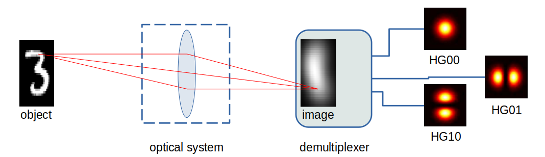
Figure 1: The left part of the figure shows a schematic representation of image formation through an optical imaging system in the far field, paraxial approximation, and in the Sub-Rayleigh regime. The right part of the figure schematically represents measurement of the field by HG SPADE. HG SPADE is a measurement strategy where the focused is processed by a spatial demultiplexer that sorts the transverse field in its Hermite-Gaussian component. Finally, each component is independently measured by photon counting. The figure shows only the lower modes $\text{HG}_{00}$, $\text{HG}_{01}$, $\text{HG}_{10}$. This is in contrast with direct imaging, where the focused image is directly measured with a camera by pixel-by-pixel photon detection.

I.1 Summary of results and relation with previous work

In this work we achieve two main goals. First, we shed light on why HG SPADE is an optimal measurement to solve estimation and discrimination problems for ultra-weak sources in the sub-Rayleigh regime. Second, we address the more general problem of learning quantum state of light, i.e., we consider a setting where minimal information is given about the source objects. We show the advantage of HG SPADE persists even in this more general setting.

The optimality of HG SPADE for parameter estimation has been shown by direct calculations and comparison with the ultimate quantum limit Tsang et al. (2016). The main theoretical tools are the Fisher information and quantum Fisher information, which bound the statistical error through the (quantum) Cramér-Rao bound Paris (2009); Sidhu and Kok (2020). Other works have shown that the optimal measurement can be constructed by taking derivative of the PSF Paúr et al. (2016), and that HG SPADE is optimal for estimating the moments of the intensity distribution of incoherent sources Zhou and Jiang (2019).

For hypothesis testing, the main theoretical tools are the Helstrom bound, the Chernoff bound, and the relative entropy. These quantities yield the optimal guessing probability and have been directly computed in recent works Grace and Guha (2022); Lu et al. (2018); Huang and Lupo (2021); Huang et al. (2023). In particular, Grace and Guha showed that the Chernoff bound can be expressed in terms of the second moments of the intensity distribution of the source objects, also showing by direct calculation the optimality of SPADE Grace and Guha (2022).

The above-mentioned works rigorously and comprehensively proved the optimality of HG SPADE and advantages with respect to DI, but somewhat lacked a simple and direct physical explanation for these results. In this work we fill this gap with a simple theory that gives a direct physical intuition of the optimality of HG SPADE. Our approach is based on expanding the state of a single photon in the sub-Rayleigh regime. This expansion shows the special role played by HG modes, from which optimality for hypothesis testing and estimation follows in a straightforward way.

Moving to the second objective of this work, we note that the problems of hypothesis testing and parameter estimation, which are those most commonly discussed in literature, refer to a somewhat contrived setting where abundant prior information is available about the scene that is observed, with one or at most a few unknown parameters. This is in contrast with most common use cases of imaging, where one has little or no prior information about the objects in the scene. For example, for the problem of parameter estimation, a commonly discussed setup is the one when one knows that there are two point-like emitters, and the goal is to estimate their spatial separation Tsang et al. (2016) (or variants of this problem Lupo et al. (2020); Krovi (2021)). In statistical hypothesis testing, two known sources are given with different geometry Grace and Guha (2022): for example a single emitter vs a pair of emitters, or two different QR codes. In summary, in all these examples the physical situation is well modeled and there is only one unknown parameter, which has continuous values in parameter estimation and discrete values in hypothesis testing (with extensions to a few parameters in multi-parameter estimation Řehaček et al. (2017); Yu and Prasad (2018); Napoli et al. (2019) and $M$-ary hypothesis test Grace and Guha (2022), respectively).

In this work we move a step forward in the direction of real-world applications of imaging, where one has only little prior information about the scene that is observed. Here we show that SPADE still outperforms DI in this more general setting. Our application can be viewed as a hybrid quantum-classical machine learning algorithm for image classification. The goal is to learn highly blurred images, generated by unknown objects sampled from a large dataset, using the data collected from a limited number of photon detection events. As a case study we use MNIST (Modified National Institute of Standards and Technology) database of handwritten digits. The physical part of our scheme is the application of HG SPADE, which implements a pre-processing of the quantum information encoded in the unknown state of a single photon. The classical part is a machine learning algorithm, which takes the measurement outputs of HG SPADE as input for training and classification

Here we simulate the physical part of the scheme, including the source emission, light propagation, and detection by HG SPADE or DI, assuming imaging through a diffraction-limited optical system (e.g., a microscope or telescope) in the regime of ultra-weak signals. The simulated data are then fed into a machine learning algorithm. Our numerical experiments show that HG SPADE combined with machine learning allows us to classify images with accuracy much above what can be achieved by DI.

I.2 Structure of the paper

In Section II we introduce the physical model and the relevant assumptions of our work. In Section III we present a theory that elucidates the special role played by the HG modes, hence explaining why HG SPADE is the optimal measurement strategy for estimation and discrimination problems. In Section IV we illustrate our numerical experiments, the results obtained and the methodology employed, with the goal of assessing the accuracy achieved by HG SPADE in learning sub-Rayleigh objects in comparison to DI. Finally, in Section V we present our conclusions and outline potential future directions of research.

II The physical model

Consider an extended source of incoherent, quasi-monochromatic light at wavelength $\lambda$. Such an object is characterised by its source intensity distribution. For example, later in our numerical experiments we choose objects from the MNIST dataset: grey-scale masks of $28\times 28$ pixels, with intensity $I_{xy}$, where $x,y$ is the pixel location in the object plane. Our physical model is schematically shown in Fig. 1.

We are interested in highly attenuated sources, emitting much less than one photon per pulse in average. In this regime, the light emitted by the object can be expressed as an incoherent sum of the vacuum and single-photon states, with density matrix

$$\rho_{0}=(1-\varepsilon)|0\rangle\langle 0|+\varepsilon\sum_{xy}I_{xy}|1_{xy}\rangle\langle 1_{xy}|\,,$$ (1)

where $\varepsilon\ll 1$ is the probability that a photon is emitted, $I_{xy}$ is the normalised intensity distribution, $|0\rangle$ is the vacuum state, and $|1_{xy}\rangle=a_{xy}^{\dagger}|0\rangle$ is the state of a single photon emitted from the pixel in $x,y$, with $a_{xy}^{\dagger}$ being the corresponding bosonic creation operator. Terms with two or more photons are negligible in the limit of ultra-weak signals. For simplicity we consider a scalar field as polarisation-related effects are out of the scope of this work.

The object is observed using an optical imaging system, which in the far field and within the paraxial approximation is characterised by its PSF, denoted $T$ Goodman (2008). The PSF is the image of a point-like source. In particular, $T(x^{\prime}-Mx,y^{\prime}-My)$ is the amplitude of the field at position $x^{\prime},y^{\prime}$ in the image plane given that it was emitted at position $x,y$ in the object plane, where $M$ is the magnification factor (to simplify the notation, from now on we put $M=1$). The particular form of the PSF depends on the details of the optical system. As a concrete example, here we consider a Gaussian PSF,

$$T(x^{\prime}-x,y^{\prime}-y)=\mathcal{N}^{1/2}e^{-\frac{(x^{\prime}-x)^{2}+(y^{\prime}-y)^{2}}{4\sigma^{2}}}\,,$$ (2)

where $\mathcal{N}^{1/2}$ is the normalisation factor.

The width of the PSF quantifies the amount of diffraction in the optical system, and is of the order of the Rayleigh length, $\sigma\simeq\mathrm{x_{R}}$. The Gaussian PSF can be used to approximate the PSF arising from a circular pupil, especially if $\sigma$ is much larger than the size of the source Santamaria et al. (2023).

The optical imaging system maps the single-photon state $|1_{xy}\rangle$ into

$$|T_{xy}\rangle:=\sum_{x^{\prime},y^{\prime}}T(x-x^{\prime},y-y^{\prime})|1_{x^{\prime}y^{\prime}}\rangle\,.$$ (3)

Therefore, the source state in Eq. (1) is mapped into the following state of the field in the image plane:

$$\rho=(1-\varepsilon)|0\rangle\langle 0|+\varepsilon\sum_{xy}I_{xy}|T_{xy}\rangle\langle T_{xy}|\,.$$ (4)

We remark that, given two point-sources at position $(x,y)$ and $(u,v)$ in the object plane, we have $\langle T_{xy}|T_{uv}\rangle\neq 0$ unless the transverse separation between the point-sources is much larger than the width of the PSF. This means that the two sources cannot be perfectly resolved.

II.1 Direct imaging

Equation (4) represents the state of the field in the image plane. This is the state that is measured to extract information about the object. DI consists of pixel-by-pixel photon detection in the image plane, which yields measurement outcomes sampled from the probability distribution

$$p_{xy}^{\text{DI}} =\varepsilon\sum_{x^{\prime}y^{\prime}}I_{x^{\prime}y^{\prime}}|\langle 1_{xy}|T_{x^{\prime}y^{\prime}}\rangle|^{2}$$ (5)

$$=\varepsilon\sum_{x^{\prime}y^{\prime}}I_{x^{\prime}y^{\prime}}|T(x-x^{\prime},y-y^{\prime})|^{2}\,,$$ (6)

whereas no photon is detected with the complementary probability $1-\varepsilon$. This probability density is the convolution of the object intensity distribution with the squared PSF. For Gaussian PSF, this is a Gaussian convolution:

$$p_{xy}^{\text{DI}}=\varepsilon\mathcal{N}\sum_{x^{\prime}y^{\prime}}I_{x^{\prime}y^{\prime}}\,e^{-\frac{(x-x^{\prime})^{2}+(y-y^{\prime})^{2}}{2\sigma^{2}}}\,.$$ (7)

Finally, we consider a finite number $N$ of photons detected. Therefore, the quantity of interest for us is the relative frequency, denoted $f_{xy}^{\text{DI}}(N)$, which is obtained by sampling (with replacement) from the probability distribution in (7).

As an example, Fig. 2 shows the original MNIST object and the relative frequencies $f_{xy}^{\text{DI}}(N)$ obtained from the simulation of $N=10^{3}$ photon detection events, in correspondence of PSF width $\sigma=4$ and $\sigma=8$ (in units of number of pixels).

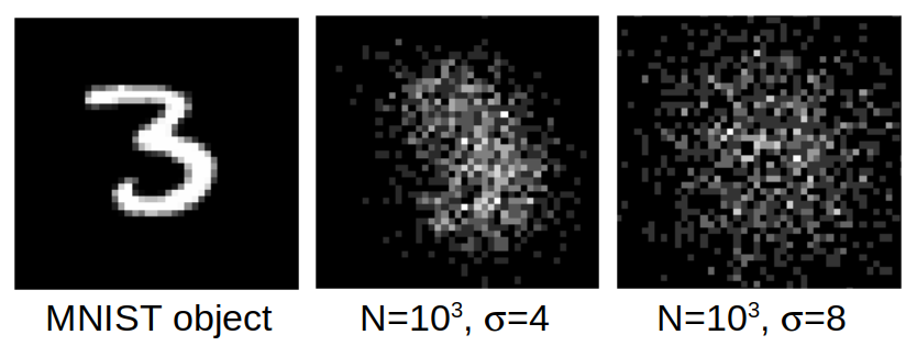
Figure 2: An example of MNIST object and the relative frequency from DI simulated for $N=10^{3}$ photon detection events. The PSF width $\sigma$ is given in number of pixels.

II.2 Spatial-mode demultiplexing

Optics offers to the experimenter much more than DI. The optical field at the image plane can in fact be measured in other ways. Among all possible detection strategies, a special role is played by SPADE, which is implemented through a linear, passive interferometer. This implies that the single-photon state in Eq. (4) is processed without increasing the average photon number. In presence of loss, there is a non-zero probability that the photon is lost and the interferometer outputs the vacuum.

Consider a basis $\{\Psi_{uv}\}_{u,v=0,1,\dots}$ of orthogonal functions in the image plane. They define a set of normal modes for the transverse field. In particular, consider the corresponding single-photon states, denoted as $|\Psi_{uv}\rangle$, that is,

$$|\Psi_{uv}\rangle:=\sum_{x,y}\Psi_{uv}(x,y)|1_{xy}\rangle\,.$$ (8)

The field can be decomposed along the $n^{2}$ lower modes by means of an interferometer with $n\times n$ output ports. A notable example is provided by HG modes, where

$$\Psi_{uv}(x,y)\equiv\text{HG}_{uv}(x,y)=\phi_{u}(x)\phi_{v}(y)\,,$$ (9)

with

$$\phi_{u}(x)=\frac{\mathcal{N}^{1/2}}{\sqrt{2^{u}u!}}\,e^{-\frac{x^{2}}{4\sigma^{2}}}H_{u}\left(\frac{x}{\sqrt{2}\sigma}\right)\,,$$ (10)

and $H_{u}$ denotes the Hermite polynomials. Note that the width $\sigma$ matches that of the Gaussian PSF, which yields the optimal choice of measurement.

Let us denote as $b_{uv}^{\dagger}$ the operator that creates a photon in the output port $(u,v)$ of the interferometer, for $u,v=1,\dots,n$. Such an interferometer, when applied to single-photon states, is represented by the operator

$$W=\sum_{uv}|1_{uv}\rangle\langle\Psi_{uv}|\,,$$ (11)

where $|1_{uv}\rangle=b_{uv}^{\dagger}|0\rangle$ is the state of a single photon in the $u,v$ output port. By mode-wise photon detection on the output ports, we obtain the probability that the photon is measured in mode $\Psi_{uv}$:

$$p_{uv}^{\text{SPADE}} =\varepsilon\sum_{xy}I_{xy}|\langle 1_{uv}|W|T_{xy}\rangle|^{2}$$ (12)

$$=\langle\Psi_{uv}|\rho|\Psi_{uv}\rangle\,,$$ (13)

with $\rho$ as in Eq. (4). A device that demultiplexes the optical field in the lower-order HG modes is schematically represented in Fig. 1.

Finally, for $N$ independent photon detection events, we need to consider the relative frequency $f_{uv}^{\text{SPADE}}(N)$, obtained by sampling with replacement from the probability distribution $p_{uv}^{\text{SPADE}}$.

III The special role played by the HG basis

To elucidate the special role played by the HG, we expand the state in the HG basis in the limit where the object size is much smaller than the Rayleigh length. This expansion will show that all relevant information is encoded in the lower HG modes.

First consider the field generated by a point-like source. This is expressed by the displaced PSF,

$$|T_{x,y}\rangle =\sum_{x^{\prime},y^{\prime}}T(x-x^{\prime},y-y^{\prime})|1_{x^{\prime},y^{\prime}}\rangle$$ (14)

$$=\mathcal{N}^{1/2}\sum_{x^{\prime},y^{\prime}}e^{-\frac{(x-x^{\prime})^{2}+(y-y^{\prime})^{2}}{4\sigma^{2}}}|1_{x^{\prime},y^{\prime}}\rangle\,,$$ (15)

where again we are assuming a Gaussian PSF. Expanding this vector in the HG basis we obtain

$$|T_{x,y}\rangle =e^{-\frac{|x|^{2}+|y|^{2}}{8\sigma^{2}}}\sum_{m,n}\frac{1}{\sqrt{m!n!}}\frac{x^{m}y^{n}}{(2\sigma)^{m+n}}|\text{HG}_{mn}\rangle\,.$$ (16)

From this we obtain the density matrix in Eq. (4), conditioned on having at least one photon (i.e., we are neglecting the vacuum contribution),

$$\rho =\sum_{x,y}I_{x,y}|T_{x,y}\rangle\langle T_{x,y}|$$ (17)

$$=\sum_{x,y}I_{x,y}e^{-\frac{|x|^{2}+|y|^{2}}{4\sigma^{2}}}\sum_{m,n}\frac{1}{\sqrt{m!n!}}\frac{x^{m}y^{n}}{(2\sigma)^{m+n}}|\text{HG}_{mn}\rangle$$ (18)

$$\phantom{=}~{}\times\sum_{m^{\prime},n^{\prime}}\frac{1}{\sqrt{m^{\prime}!n^{\prime}!}}\frac{x^{m^{\prime}}y^{n^{\prime}}}{(2\sigma)^{m^{\prime}+n^{\prime}}}\langle\text{HG}_{m^{\prime}n^{\prime}}|$$ (19)

$$=\sum_{x,y}I_{x,y}e^{-\frac{|x|^{2}+|y|^{2}}{4\sigma^{2}}}$$

$$\phantom{=}~{}\times\sum_{mm^{\prime}nn^{\prime}}\frac{x^{m+m^{\prime}}y^{n+n^{\prime}}}{(2\sigma)^{m+m^{\prime}+n+n^{\prime}}}\frac{|\text{HG}_{mn}\rangle\langle\text{HG}_{m^{\prime}n^{\prime}}|}{\sqrt{m!m^{\prime}!n!n^{\prime}!}}\,.$$ (20)

Consider now the sub-Rayleigh regime. In this limit we can truncate the expansion up to the second order in $x/\sigma$ and $y/\sigma$. This yields

$$\rho \simeq\left(1-\frac{\langle x^{2}\rangle+\langle y^{2}\rangle}{4\sigma^{2}}\right)|\text{HG}_{00}\rangle\langle\text{HG}_{00}|$$

$$\phantom{=}~{}+\frac{\langle x\rangle}{2\sigma}\left(|\text{HG}_{00}\rangle\langle\text{HG}_{10}|+|\text{HG}_{10}\rangle\langle\text{HG}_{00}|\right)$$

$$\phantom{=}~{}+\frac{\langle y\rangle}{2\sigma}\left(|\text{HG}_{00}\rangle\langle\text{HG}_{01}|+|\text{HG}_{01}\rangle\langle\text{HG}_{00}|\right)$$

$$\phantom{=}~{}+\frac{\langle x^{2}\rangle}{4\sigma^{2}}|\text{HG}_{10}\rangle\langle\text{HG}_{10}|+\frac{\langle y^{2}\rangle}{4\sigma^{2}}|\text{HG}_{01}\rangle\langle\text{HG}_{01}|$$

$$\phantom{=}~{}+\frac{\langle xy\rangle}{4\sigma^{2}}\left(|\text{HG}_{10}\rangle\langle\text{HG}_{01}|+|\text{HG}_{01}\rangle\langle\text{HG}_{10}|\right)\,,$$ (21)

where $\langle x^{2}\rangle:=\sum_{x,y}I_{x,y}x^{2}$, $\langle xy\rangle:=\sum_{x,y}I_{x,y}xy$, etc.

This expansion shows that in the sub-Rayleigh regime the state is completely determined by the first and second moments of the intensity distribution.

A further simplification is obtained if we assume that the optical system is aligned towards the “center of mass” (defined using the intensity as weights) of the source object. This means that the first moments vanish,

$$\langle x\rangle=\langle y\rangle=0\,,$$ (22)

and the state in Eq. (21) becomes block-diagonal, that is, the cross-terms $|\text{HG}_{00}\rangle\langle\text{HG}_{10}|$, $|\text{HG}_{00}\rangle\langle\text{HG}_{01}|$ are suppressed.

In conclusion, the state of a single photon emitted by the source, in the sub-Rayleigh regime and if the optical system is aligned to the “center of mass”, is completely determined by the covariance matrix of the intensity distribution,

$$\gamma=\sum_{x,y}I_{x,y}\left(\begin{array}[]{cc}x^{2}&xy\\ xy&y^{2}\end{array}\right)\,.$$ (25)

Note that photon detection in the modes $\text{HG}_{01}$ and $\text{HG}_{10}$ directly estimates the second order moments. To estimate the off-diagonal terms we need to rotate the HG modes. A rotation of the optical system of an angle $\varphi$ defines the rotated HG modes

$$|\text{HG}_{01}(\varphi)\rangle =\cos{\varphi}|\text{HG}_{01}\rangle-\sin{\varphi}|\text{HG}_{10}\rangle$$ (26)

$$|\text{HG}_{10}(\varphi)\rangle =\sin{\varphi}|\text{HG}_{01}\rangle+\cos{\varphi}|\text{HG}_{10}\rangle\,.$$ (27)

For a particular choice of $\varphi$ the covariance matrix becomes diagonal. Therefore, photon detection in the lower HG modes, rotated by a suitable angle, completely determines the source in the sub-Rayleigh regime.

III.1 Symmetric binary discrimination

In binary classification, two source objects are given, which determine two corresponding states of light, $\rho_{0}$ and $\rho_{1}$. As we have seen above, in the sub-Rayleigh regime these states are equivalently represented by the intensity covariance matrices $\gamma_{0}$ and $\gamma_{1}$.

In the framework of symmetric discrimination, one considers the average probability of obtaining a false positive or a false negative. The fundamental limit on such a probability is given by the Helstrom bound Helstrom (1976), which expresses the minimum average error probability in terms of the trace distance between the states $\rho_{0}$ and $\rho_{1}$, or equivalently between the covariance matrices $\gamma_{0}$ and $\gamma_{1}$,

$$P_{\text{err}}=\frac{1-\Delta}{2}\,,$$ (28)

where

$$\Delta=\frac{1}{2}\|\rho_{0}-\rho_{1}\|_{1}=\frac{\varepsilon}{8\sigma^{2}}\left(\delta+\|\gamma_{0}-\gamma_{1}\|_{1}\right)\,,$$ (29)

and $\|\,\cdot\,\|_{1}=\mathrm{Tr}|\,\cdot\,|$ denotes the $1$-norm, and

$$\delta=\left|\mathrm{Tr}\gamma_{0}-\mathrm{Tr}\gamma_{1}\right|\,.$$ (30)

It is known that the optimal measurement that saturates the Helstrom bounds corresponds to projections into the positive and negative parts of the difference $\rho_{0}-\rho_{1}$, which in our setting is equivalent to the projectors onto the positive and negative parts of $\gamma_{0}-\gamma_{1}$. Since $\gamma_{0}-\gamma_{1}$ is a $2\times 2$ matrix, each of these projector is a one-dimensional projector corresponding to the eigenvectors of $\gamma_{0}-\gamma_{1}$. We can then distinguish two cases:

1. If the matrices $\gamma_{0}$ and $\gamma_{1}$ commute, then they share a common pair of eigenvectors, which are obtained for a particular choice of the rotation angle $\varphi$ in Eqs. (26)-(27). Such value of the angle is determined by the common axes of symmetry of the objects. In turn, the projectors into the positive and negative part of $\gamma_{0}-\gamma_{1}$ corresponds to rotated HG states and the optimal measurement is HG detection along the angle $\varphi$.

2. If the matrices do not commute, we need to consider the eigenvectors of $\gamma_{0}-\gamma_{1}$. Without loss of generality, the eigenvectors are once again of the form in Eqs. (26)-(27) for some specific value of $\varphi$. Therefore also in this case detection in rotated HG modes is optimal.

In conclusion, we have obtained the following result concerning sub-Rayleigh image discrimination:

Proposition 1

Photon detection in the rotated HG modes saturates the Helstrom bound for ultra-weak signals in the sub-Rayleigh regime.

III.2 Estimation of the moments

Consider a quantum state $\rho(\vartheta)$ depending on an unknown parameter $\vartheta$. The goal of parameter estimation is to estimate $\vartheta$ by measuring $N$ instances of the state.

In the context of imaging, Tsang and collaborators showed in Ref. Tsang et al. (2016) that DI is not suitable for parameter estimation when the size of the object is much smaller than the Rayleigh length. They showed that the statistical error in the estimation becomes unbounded in the sub-Rayleigh limit. This phenomenon, dubbed the Rayleigh curse, is the manifestation of the Rayleigh resolution criterion in the context of parameter estimation.

In the same work, Tsang and collaborators also showed that HG SPADE lifts the Rayleigh curse, allowing parameter estimation with a statistical error that does not depend on the size of the object. HG SPADE also saturates the ultimate quantum limit as expressed by the quantum Cramér-Rao bound. The problem considered in Ref. Tsang et al. (2016) was the estimation of the transverse separation $s$ between two point-like sources. Similar conclusions were also drawn by Zhou and Jiang Zhou and Jiang (2019) for the estimating of the second moments of the intensity distribution of a two-dimensional incoherent source laying in the object plane.

Consider the moments of order $k$:

$$M_{i,j}=\sum_{x,y}I_{x,y}x^{i}y^{j}\,,$$ (31)

with $i+j=k$, and define the parameters

$$\vartheta_{i,j}:=\sqrt{M_{i,j}}$$ (32)

as the square root of the moments. Note that for the case of two point-sources of equal intensity, with transverse separation $s$ along the $x$-axis, and if the optical system is aligned to the mid-point, we obtain $s^{2}=4M_{2,0}$ and $s=2\vartheta_{2,0}$. Therefore, the estimation of the parameters $\vartheta_{i,j}$ includes the original problem of Tsang and collaborators as a special case.

We now show why HG SPADE allows us to lift the Rayleigh curse for the estimation of the separation $s$, and more generally for the estimation of the parameters $\vartheta_{i,j}$. Consider first the estimation of $\vartheta_{2,0}=\sqrt{\langle x^{2}\rangle}$. According to the decomposition in HG basis in Eq. (21), the moments of order two are proportional to the probability of detecting a photon in the lower HG modes. For example, photon detection in $\text{HG}_{10}$ has probability

$$p_{10}=\frac{\varepsilon}{4\sigma^{2}}\langle x^{2}\rangle\,.$$ (33)

It follows from the properties of the binomial distribution that, given $N$ photon detection events, the statistical error in the estimation of $p_{10}$ is

$$\Delta p_{10}=\sqrt{\frac{p_{10}(1-p_{10})}{N}}\,,$$ (34)

which also saturates the Cramér-Rao bound. In the sub-Rayleigh limit, we have $p_{10}\ll 1$, therefore

$$\Delta p_{10}\simeq\sqrt{\frac{p_{10}}{N}}\,.$$ (35)

By error propagation, from this we obtain the statistical error in the estimation of $\sqrt{p_{10}}$:

$$\Delta\sqrt{p_{10}}\simeq\frac{1}{2}\sqrt{\frac{1}{N}}\,,$$ (36)

and finally the error in the estimation of the parameter $\vartheta_{2,0}=2\sigma\sqrt{p_{10}/\varepsilon}$:

$$\Delta\vartheta_{2,0}\simeq\sigma\sqrt{\frac{1}{\varepsilon N}}\,.$$ (37)

(Note that $\varepsilon N$ is the average number of photons detected.)

We can actually generalise this result. From the HG expansion in Eq. (20) we see that photon detection in modes $\text{HG}_{mn}$ is related to the even moments $\langle x^{2m}y^{2n}\rangle$. Reasoning as above we conclude that the Rayleigh curse is lifted for the estimation of the parameters $\vartheta_{2m,2n}=\sqrt{\langle x^{2m}y^{2n}\rangle}$.

In conclusion, we have obtained the following result:

Proposition 2

Photon detection in HG modes lifts the Rayleigh curse for the estimation of the square root of all even moments, $\vartheta_{2m,2n}=\sqrt{\langle x^{2m}y^{2n}\rangle}$. Furthermore, the parameters $\vartheta_{2m,2n}$ can be jointly estimated with a single HG SPADE measurement.

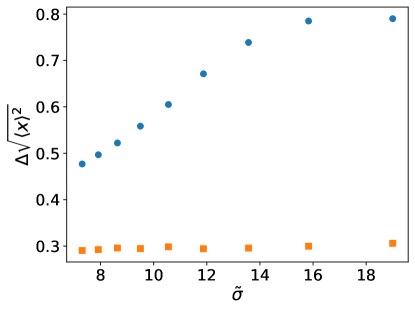
Figure 3: Statistical error $\Delta\sqrt{\langle x^{2}\rangle}$ obtained from simulated $N=10^{3}$ photon detection events, plotted versus the noise parameter $\tilde{\sigma}=\sigma/f$, where $\sigma=9.5$ pixels and $f$ is a scaling factor. The blue dots are for DI, where the square root of the second moment $\vartheta_{2,0}=\sqrt{\langle x^{2}\rangle}$ is computed using Eq. (38). The orange squares are for SPADE, where the estimated quantity is $\sqrt{p_{10}}$. We note that the error from DI increases with increasing $\tilde{\sigma}$, whereas the error from SPADE remains constant.

Since it allows for a direct estimation of (the square root of) the even moments, it is natural to expect HG SPADE to outperform DI for this task. In fact, to obtain the moments from DI we first need photon detection in each pixel to estimate the quantities $p_{xy}^{\text{DI}}$ in Eq. (7). For example, to estimate the quantity $\langle x^{2}\rangle$, we need to combine them in the formula:

$$\langle x^{2}\rangle=\sum_{x,y}x^{2}p_{xy}^{\text{DI}}-\sigma^{2}\,,$$ (38)

where the terms $\sigma^{2}$ account for de-convolution of the Gaussian blurring. As errors propagate and accumulate, we expect a lower signal-to-noise ratio when estimating $\vartheta_{2,0}$ using data collected by DI.

We have numerically verified this by considering an object from the MNIST data set (the one in Fig. 2), re-scaling it by a factor $1/f$, and then applying a Gaussian noise with width $\sigma$. The effects of diffraction are quantified by quantity $\tilde{\sigma}=\sigma/f$. Since the original MNIST image is pixelated, aliasing errors occur when the image is re-scaled. We have selected a range of values of $f$ such that the aliasing error has only a limited impact. A comparison between the statistical error $\Delta\sqrt{\langle x^{2}\rangle}$ in the estimation of $\vartheta_{2,0}=\sqrt{\langle x^{2}\rangle}$ with DI and SPADE is shown in Fig. 3.

IV Numerical experiments

In this Section we present a number of numerical experiments where HG SPADE is combined with machine learning algorithms into a hybrid quantum-classical approach to classify faint sources in the sub-Rayleigh regime. The dataset used for the experiments is the MNIST, handwritten digits, which is extracted from the torchvision Python library. This is a widesrpread benchmark dataset in computer vision and machine learning.

First we simulate the action of the optical imaging system, which focuses the field emitted from the object sources. For experiments of binary classification, we consider restricted datasets of either $0$’s and $1$’s (in Section IV.1) or $6$’s and $9$’s (in Section IV.1). All classes of MNIST objects, i.e. the digits from zero to nine, are considered in Section IV.2. Diffraction through the pupil of the optical system induces blurring. In our simulation we fix the value of the width of the PSF to $\sigma=9.5$ (measured in number of pixels), and scale the source object by a factor $f$: this induces a relative width of $\tilde{\sigma}=\sigma/f$. From the focused optical field we can compute the probability of photon detection for both DI and HG SPADE, respectively using Eq. (7) and Eq. (12). The statistics for given number of detected photon $N$ is generated by Monte Carlo simulation.

Finally, the datasets obtained in this way are directly ingested into a machine learning model trained for classification. The models used in the following for performing the classification are standard ones in the machine learning literature: Random Forest Breiman (2001) and Fully Connected Neural Network (FCNN) Goodfellow et al. (2016). RF is an ensemble learning methods that proves to be quite effective both in regression and in classification. Furthermore, it is relativity light, hence, given the size of the HG SPADE vector, it is expected to capture the fundamental features useful for the classification. FCNN on the contrary is a deep learning method, particularly used for classification, that extracts features from the input sample via a series of connected hidden layers with non-linear activation functions. It is one of the standard models for automated classification, particularly useful in computer vision.

IV.1 Binary classification

The first problem we consider is the binary classification of MNIST objects from the classes of $0$’s and $1$’s. Elements belonging to these two classes are well separated in terms of the second moments of their intensity. Figure 4 shows the distribution of second moments for a sample of $300$ objects from the database. the figure shows the moments in both the Cartesian basis,

$$\langle x^{2}\rangle =\sum_{x,y}I_{x,y}x^{2}\,,$$ (39)

$$\langle y^{2}\rangle =\sum_{x,y}I_{x,y}y^{2}\,,$$ (40)

and in the diagonal basis (obtained by rotation of $45^{\circ}$ degrees),

$$\frac{1}{2}\langle(x+y)^{2}\rangle =\frac{1}{2}\sum_{x,y}I_{x,y}(x+y)^{2}\,,$$ (41)

$$\frac{1}{2}\langle(x-y)^{2}\rangle =\frac{1}{2}\sum_{x,y}I_{x,y}(x-y)^{2}\,.$$ (42)

Note that the MNIST objects are already centered in such a way that $\langle x\rangle=\langle y\rangle=0$.

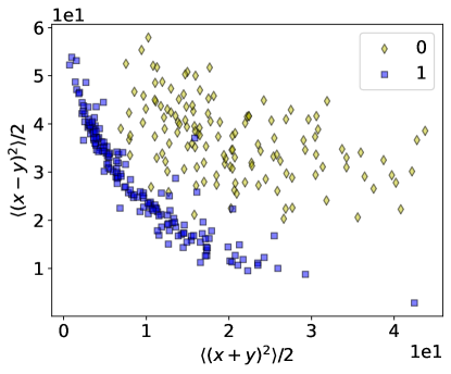
Figure 4: Scatter plot of the second moments of a sample of $300$ objects from the MNIST classes $0$ and $1$. Top: the moments are computed in the Cartesian basis, according to Eqs. (39)-(40). Bottom: moments in the diagonal basis, computed as in Eqs. (41)-(42).

IV.1.1 SPADE

We have seen that SPADE allows us to optimally estimate the second moments. Therefore, we expect SPADE to be a good measurement choice for this particular classification problem.

We focus on SPADE in the diagonal basis, since moments in this basis appear to be more effective in separating the two classes, as shown in Fig. 4. The probability of detecting a photon in the lower diagonal modes $\text{HG}_{10}$, $\text{HG}_{01}$ can be computed directly (up to normalisation) from Eq. (20). Without taking the limit of $x/\sigma,y/\sigma\ll 1$ we obtain

$$p_{00}^{\text{SPADE}} =\sum_{x,y}I_{x,y}e^{-\frac{|x|^{2}+|y|^{2}}{4\sigma^{2}}}\,,$$ (43)

$$p_{10}^{\text{SPADE}} =\frac{1}{8\sigma^{2}}\sum_{x,y}I_{x,y}(x+y)^{2}e^{-\frac{|x|^{2}+|y|^{2}}{4\sigma^{2}}}\,,$$ (44)

$$p_{01}^{\text{SPADE}} =\frac{1}{8\sigma^{2}}\sum_{x,y}I_{x,y}(x-y)^{2}e^{-\frac{|x|^{2}+|y|^{2}}{4\sigma^{2}}}\,.$$ (45)

For any given integer value for the photon number $N$, we have implemented a MonteCarlo simulation to generate the relative frequencies $f_{uv}^{\text{SPADE}}(N)$ (see Section II.2) by sampling (with replacement) from the above distribution $p_{uv}^{\text{SPADE}}$. We have tested a RF using these relative frequencies as feature vectors. With a sample of $11867$ images from the database, and using $70\%$ of them for training and $30\%$ for validation. The results are displayed in Fig. 5, which shows the accuracy vs the PSF width $\tilde{\sigma}$, for different values of the photon number $N$.

Figure 5 shows the qualitative behaviours of the accuracy: (1) the accuracy decreases with increasing $\tilde{\sigma}$, as the Gaussian noise induced by diffraction makes more difficult to discriminate the objects; (2) the accuracy increases with increasing $N$, due to smaller statistical fluctuations.

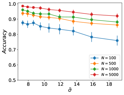
Figure 5: Accuracy for binary classification of $0$’s and $1$’s using RF, performed on the HG SPADE vectors, evaluated in a rotated basis. The results are evaluated for different effective blurring factors $\tilde{\sigma}=9.5/f$ and considering various values of the number of photon detection events, $N$ (from bottom to topo, $N=100,500,1000,5000$). The error bars are calculated via stratified $k$-fold Ojala and Garriga (2010), using $m=10$ splits of the test dataset.

Figure 6: Accuracy for the binary classification of $0$’s and $1$’s, performed on the simulated DI (a) with RF, (b) with FCNN, (c) with RF on second moments computed from DI data. The results are evaluated for different effective blurring factors $\tilde{\sigma}=9.5/f$ and considering various photon detection events, $N$ (from bottom to top, $N=100,500,1000,5000$). The error bars are calculated via stratified $k$-fold Ojala and Garriga (2010), using $m=10$ splits of the test dataset.

IV.1.2 DI

To compare with SPADE, we have performed a similar analysis for DI. For any number $N$ of photon detection events, we have generated the relative frequencies $f_{xy}^{\text{DI}}(N)$ (see Section II.1) by sampling (without replacement) from the DI probability distribution in Eq. (7). We have tested the machine learning approaches, with results displayed in Fig. 6. The top panel shows the results obtained for RF using the relative frequencies as feature vectors. The middles panel is for a FCNN, also using the relative frequencies as feature vectors. A direct comparison suggests that the FCNN performs much better than RF for this problem, as the hidden neurons are able to extract relevant features out of the original sample. We argue that, in particular, the FCNN is able to obtain the information most likely related to the moments of order two, which is crucial to classify correctly in the sub-Rayleigh regime.

Finally, also for a fair comparison with SPADE, we helped the algorithm by performing a pre-computation of the second moments. Starting from the relative frequencies $f_{xy}^{\text{DI}}(N)$, the second moments can be estimated as follows:

$$\langle x^{2}\rangle \leftarrow\sum_{x,y}f_{xy}^{\text{DI}}(N)x^{2}\,,$$ (46)

$$\langle y^{2}\rangle \leftarrow\sum_{x,y}f_{xy}^{\text{DI}}(N)y^{2}\,,$$ (47)

for the Cartesian basis, and

$$\frac{1}{2}\langle(x+y)^{2}\rangle \leftarrow\frac{1}{2}\sum_{x,y}f_{xy}^{\text{DI}}(N)(x+y)^{2}\,,$$ (48)

$$\frac{1}{2}\langle(x-y)^{2}\rangle \leftarrow\frac{1}{2}\sum_{x,y}f_{xy}^{\text{DI}}(N)(x-y)^{2}\,,$$ (49)

for the diagonal one. In particular, we have used the estimates of the second moments in diagonal basis and used them as feature vectors in a RF. The results are displayed in the bottom panel of Fig. 6, showing an increase in the accuracy compared to the FCNN fed with the relative frequencies. Moreover, it can be noticed that the fluctuations for each $\tilde{\sigma}$ are more contained compared to the previous cases: this is due to the fact that the second moments, which now are structured within the feature vector, are independent of $\tilde{\sigma}$ and hence they stabilise the computation.

In conclusion, DI supported by either RF and FCNN yields poor performances when compared against SPADE supported by RF. The accuracy of DI increases when the second moments are pre-computed from the DI relative frequencies and fed into a RF. This latter approach mimics the pre-processing implemented by SPADE, though in a physical rather than computational way. However, also this latter approach performs poorly in comparison with SPADE, especially for low photon number. This is due to the fact that computing the moments from the data obtained by DI yields a signal-to-noise ratio smaller than a direct measurement of SPADE Santamaria et al. (2023).

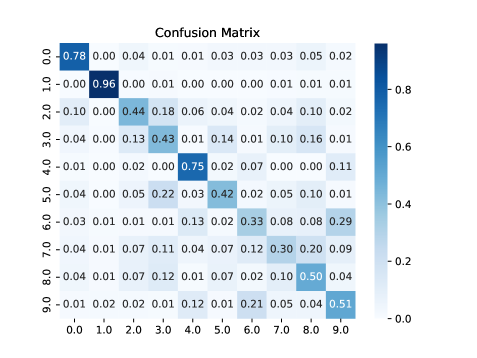
Figure 7: Confusion matrix of the output of the RF for multi-class classification, performed on the HG SPADE vectors. In particular the figure refers to the case with an effective blurring factor $\tilde{\sigma}=10$ and with number of photon detection events $N=5000$.

IV.2 Multiple classes

In this Section we present results beyond binary classification. We consider MNIST objects from all classes of digits from $0$ to $9$. To test the accuracy of SPADE for this multi-class problem we considered as features the moments of order two in both the Cartesian [see Eqs. (39)-(40)] and diagonal bases [Eqs. (41)-(42)]. In our Monte Carlo simulations, we assume that upon $N$ photon detected, half are measured in the Cartesian basis and half in the diagonal basis.

The obtained confusion matrix is shown in Fig. 7 for $N=5000$ and $\tilde{\sigma}=10$, where each row is associated with the ground truth and the columns represent the guessed class. The matrix shows mixed results. As expected, SPADE is able to discriminate very well between $0$’s and $1$’s. However, a lower accuracy is obtained for other digits. An example is given by the classes of $6$’s and $9$’s which are essentially indistinguishable from their second moments. This result is easily explained by noticing that, whereas the $0$’s and $1$’s are well separated by the second moments, this is not in general the case for the other digits. This suggests that we may need to go beyond the second moments, i.e., include in our simulation and detection HG modes of higher degrees above $\text{HG}_{01}$ and $\text{HG}_{10}$.

IV.3 Higher moments

To extend the use of SPADE beyond binary classification, we come back to the expansion of the quantum states in the HG basis in Eq. (20):

$$\rho =\sum_{x,y}I_{x,y}e^{-\frac{|x|^{2}+|y|^{2}}{4\sigma^{2}}}$$

$$\phantom{=}~{}\times\sum_{mm^{\prime}nn^{\prime}}\frac{x^{m+m^{\prime}}y^{n+n^{\prime}}}{(2\sigma)^{m+m^{\prime}+n+n^{\prime}}}\frac{|\text{HG}_{mn}\rangle\langle\text{HG}_{m^{\prime}n^{\prime}}|}{\sqrt{m!m^{\prime}!n!n^{\prime}!}}\,,$$ (50)

and keep the terms up to the fourth order in $x/\sigma$ and $y/\sigma$.

The expansion includes basis vectors $|\text{HG}_{20}\rangle$, $|\text{HG}_{11}\rangle$, $|\text{HG}_{02}\rangle$. We obtain

$$\rho \simeq\left(1-\frac{\langle x^{2}\rangle+\langle y^{2}\rangle}{(2\sigma)^{2}}-\frac{\langle x^{4}\rangle+\langle x^{2}y^{2}\rangle+\langle y^{4}\rangle}{(2\sigma)^{4}}\right)|\text{HG}_{00}\rangle\langle\text{HG}_{00}|$$ (51)

$$+\frac{\langle x^{2}\rangle}{(2\sigma)^{2}}\left(|\text{HG}_{10}\rangle\langle\text{HG}_{10}|+\frac{|\text{HG}_{00}\rangle\langle\text{HG}_{20}|+\text{h.c.}}{\sqrt{2}}\right)+\frac{\langle y^{2}\rangle}{(2\sigma)^{2}}\left(|\text{HG}_{01}\rangle\langle\text{HG}_{01}|+\frac{|\text{HG}_{00}\rangle\langle\text{HG}_{02}|+\text{h.c.}}{\sqrt{2}}\right)$$ (52)

$$+\frac{\langle xy\rangle}{(2\sigma)^{2}}\left(|\text{HG}_{00}\rangle\langle\text{HG}_{11}|+|\text{HG}_{01}\rangle\langle\text{HG}_{10}|+\text{h.c.}\right)$$ (53)

$$+\frac{\langle x^{3}\rangle}{(2\sigma)^{3}}\left(\frac{|\text{HG}_{10}\rangle\langle\text{HG}_{20}|}{\sqrt{2}}+\text{h.c.}\right)+\frac{\langle x^{2}y\rangle}{(2\sigma)^{3}}\left(|\text{HG}_{10}\rangle\langle\text{HG}_{11}|+\frac{|\text{HG}_{01}\rangle\langle\text{HG}_{20}|}{\sqrt{2}}+\text{h.c.}\right)$$ (54)

$$+\frac{\langle xy^{2}\rangle}{(2\sigma)^{3}}\left(|\text{HG}_{01}\rangle\langle\text{HG}_{11}|+\frac{|\text{HG}_{10}\rangle\langle\text{HG}_{02}|}{\sqrt{2}}+\text{h.c.}\right)+\frac{\langle y^{3}\rangle}{(2\sigma)^{3}}\left(\frac{|\text{HG}_{01}\rangle\langle\text{HG}_{02}|}{\sqrt{2}}+\text{h.c.}\right)$$ (55)

$$+\frac{\langle x^{4}\rangle}{(2\sigma)^{4}}\frac{|\text{HG}_{20}\rangle\langle\text{HG}_{20}|}{2}+\frac{\langle x^{3}y\rangle}{(2\sigma)^{4}}\frac{|\text{HG}_{11}\rangle\langle\text{HG}_{20}|+\text{h.c.}}{\sqrt{2}}$$ (56)

$$+\frac{\langle x^{2}y^{2}\rangle}{(2\sigma)^{4}}\left(|\text{HG}_{11}\rangle\langle\text{HG}_{11}|+\frac{|\text{HG}_{20}\rangle\langle\text{HG}_{02}|+\text{h.c.}}{2}\right)$$ (57)

$$+\frac{\langle xy^{3}\rangle}{(2\sigma)^{4}}\frac{|\text{HG}_{11}\rangle\langle\text{HG}_{02}|+\text{h.c.}}{\sqrt{2}}+\frac{\langle y^{4}\rangle}{(2\sigma)^{4}}\frac{|\text{HG}_{02}\rangle\langle\text{HG}_{02}|}{2}\,.$$ (58)

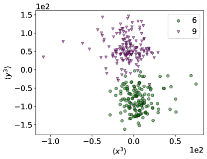
Figure 8: Scatter plot of the third moments of a sample of $300$ objects from the MNIST classes $6$ and $9$.

By applying suitable measurements to the above state, one can obtain information about all the moments of the source intensity distribution up to the fourth order. As a concrete example, we focus on the problem of classifying MNIST objects belonging to the classes of $6$’s and $9$’s. Objects from these classes have essentially the same distribution of the second moments. Therefore, SPADE in the lower-order HG modes cannot classify them, as shown by the confusion matrix in Fig. 7. However, they are well separated by the third moments, as seen from Fig. 8. This suggests to extract information about the third moments $\langle x^{3}\rangle$ and $\langle y^{3}\rangle$ from the HG measurements. However, photon detection in the HG SPADE modes does not allow us to access the moments of the third order. We need to consider linear combinations of the HG basis elements. We consider the six vectors (this choice is not necessarily optimal, but provides a way to extract information about the third moments):

$$\left\{|\text{HG}_{00}\rangle,\frac{|\text{HG}_{01}\rangle\pm|\text{HG}_{02}\rangle}{\sqrt{2}},\frac{|\text{HG}_{10}\rangle\pm|\text{HG}_{20}\rangle}{\sqrt{2}},|\text{HG}_{11}\rangle\right\}\,.$$ (59)

Photon detection in these states is associated to the probabilities

$$|\text{HG}_{00}\rangle\to 1-\frac{\langle x^{2}\rangle+\langle y^{2}\rangle}{(2\sigma)^{2}}-\frac{\langle x^{4}\rangle+\langle x^{2}y^{2}\rangle+\langle y^{4}\rangle}{(2\sigma)^{4}}\,,$$ (60)

$$\frac{|\text{HG}_{01}\rangle\pm|\text{HG}_{02}\rangle}{\sqrt{2}}\to\frac{1}{2}\left(\frac{\langle y^{2}\rangle}{(2\sigma)^{2}}+\frac{\langle y^{4}\rangle}{2(2\sigma)^{4}}\pm\frac{\sqrt{2}\langle y^{3}\rangle}{(2\sigma)^{3}}\right)\,,$$ (61)

$$\frac{|\text{HG}_{10}\rangle\pm|\text{HG}_{20}\rangle}{\sqrt{2}}\to\frac{1}{2}\left(\frac{\langle x^{2}\rangle}{(2\sigma)^{2}}+\frac{\langle x^{4}\rangle}{2(2\sigma)^{4}}\pm\frac{\sqrt{2}\langle x^{3}\rangle}{(2\sigma)^{3}}\right)\,,$$ (62)

$$|\text{HG}_{11}\rangle\to\frac{\langle x^{2}y^{2}\rangle}{(2\sigma)^{4}}\,.$$ (63)

A partial optimisation could be obtained by introducing an angle of rotation:

$$\sin{\varphi}|\text{HG}_{01}\rangle+\cos{\varphi}|\text{HG}_{02}\rangle\to$$

$$(\sin{\varphi})^{2}\frac{\langle y^{2}\rangle}{(2\sigma)^{2}}+(\cos{\varphi})^{2}\frac{\langle y^{4}\rangle}{2(2\sigma)^{4}}+\sqrt{2}\sin{\varphi}\cos{\varphi}\frac{\langle y^{3}\rangle}{(2\sigma)^{3}}\,,$$ (64)

$$\cos{\varphi}|\text{HG}_{01}\rangle-\sin{\varphi}|\text{HG}_{02}\rangle\to$$

$$(\cos{\varphi})^{2}\frac{\langle y^{2}\rangle}{(2\sigma)^{2}}+(\sin{\varphi})^{2}\frac{\langle y^{4}\rangle}{2(2\sigma)^{4}}-\sqrt{2}\sin{\varphi}\cos{\varphi}\frac{\langle y^{3}\rangle}{(2\sigma)^{3}}\,.$$ (65)

The angle $\varphi$ can be optimised to maximise the signal-to-noise ratio, where the signal is represented by the moment of order three and the noise by the moments of order two and four. By putting

$$\sin{\varphi} =\frac{2\sigma}{\sqrt{(2\sigma)^{2}+2(2\sigma)^{4}}}\,,$$ (66)

$$\cos{\varphi} =\frac{\sqrt{2}(2\sigma)^{2}}{\sqrt{(2\sigma)^{2}+2(2\sigma)^{4}}}\,,$$ (67)

we obtain

$$\sin{\varphi}|\text{HG}_{01}\rangle+\cos{\varphi}|\text{HG}_{02}\rangle\to\frac{y^{2}+y^{4}+2y^{3}}{(2\sigma)^{2}+2(2\sigma)^{4}}\,,$$ (68)

$$\cos{\varphi}|\text{HG}_{01}\rangle-\sin{\varphi}|\text{HG}_{02}\rangle\to\frac{2(2\sigma)^{2}y^{2}+\frac{y^{4}}{2(2\sigma)^{2}}-2y^{3}}{(2\sigma)^{2}+2(2\sigma)^{4}}\,.$$ (69)

In our simulation, we use the above states, but we do not enforce the limit of small $x/\sigma$ and $y/\sigma$. This implies that exponential terms $e^{-\frac{-|x|^{2}-|y|^{2}}{4\sigma^{2}}}$ in (IV.3) are not replaced by $1$. Finally, to ensure a proper normalisation, we also include in the simulation the probabilities of detecting a photon in the higher-order terms

$$\text{HG}_{03} \to\frac{\langle y^{6}\rangle}{(2\sigma)^{6}}\frac{1}{6}\,,$$ (70)

$$\text{HG}_{12} \to\frac{\langle x^{2}y^{4}\rangle}{(2\sigma)^{6}}\frac{1}{2}\,,$$ (71)

$$\text{HG}_{21} \to\frac{\langle y^{2}x^{4}\rangle}{(2\sigma)^{6}}\frac{1}{2}\,,$$ (72)

$$\text{HG}_{30} \to\frac{\langle x^{6}\rangle}{(2\sigma)^{6}}\frac{1}{6}\,.$$ (73)

The results of our numerical experiments are shown in Fig. 9. First we have applied this modified SPADE using the above six features (with the optimised angle $\varphi$), with $N$ photon detection events, in a RF model. The accuracy is lower than in the case of $0$’s vs $1$’s, and it requires many more detection events (higher values of $N$). This is because the third-order moments are suppressed by a factor proportional to $\tilde{\sigma}^{-3}$. With increasing $\tilde{\sigma}$, it is much less likely that is detected in an HG mode of higher degree, as most of them end up in the lower HG modes.

We then compare with DI, powered by FCNN. For small values of $\tilde{\sigma}$, DI works better than SPADE, but for larger values of $\tilde{\sigma}$ SPADE has better performance in terms of both accuracy and stability. Overall, this modified SPADE remains superior in the deep sub-Rayleigh regime (large values of $\tilde{\sigma}$), but more photon detection events are needed to acquire a decent signal-to-noise ratio.

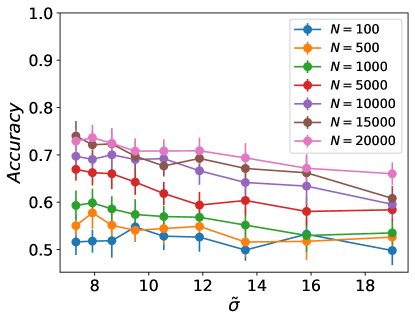
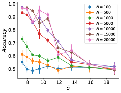
Figure 9: Accuracy vs blurring parameter $\tilde{\sigma}$ for the classification of $6$’s and $9$’s. This is shown for several values of the number of detected photon, from bottom to top $N=100,500,1000,5000,10000,15000,20000$. Top panel: data collected using the modified SPADE defined in Section IV.3, and processed using a RF. Bottom panel: data collected using DI, and processed using FCNN.

IV.4 Methodology

IV.4.1 MNIST Dataset

The full MNIST dataset, provided by the open access library torchvision, consists of a collection of handwritten digits, with $70k$ samples. Each sample is a grayscale image of size $28\times 28$ pixels, representing a single digit, with nominal pixel values ranging from $0$ to $255$. The dataset is widely considered a benchnmark for testing various machine learning and artificial intelligence algorithms, particularly those dedicated to image classification tasks. Even though it serves as a baseline, the MNIST dataset entails a diverse range of digit variations, including different writing styles, sizes and orientation. Hence it poses several challenges, such as variability in writing quality, noise and digit overlapping, making it an interesting test-bed for evaluating the effectiveness of the proposed methodologies. In this work, we make use of RF algorithm and FCNN, for evaluating the information content, and thus the performances in the classification, for the HG SPADE vectors and for the DI approach, as a function of various finite photon detection events and within a range of physical parameters.

For each model used in the experimental phase, the accuracy of the predictions is calculated by comparing them with the true labels in the test set:

$$\text{Accuracy}=\frac{N_{c}}{N_{T}}\,,$$ (74)

where $N_{c}$ is the number of correct prediction, while $N_{T}$ is the total number of predictions. The effectiveness of the SPADE technique is assessed based on the improvement in classification accuracy, in case of extreme blurring, compared to the results when the direct intensity features are used.

IV.4.2 Data Preprocessing and Models Architecture

For binary classification, starting from the full MNIST dataset we consider the reduced problem of binary classification: out of the $10$ classes, corresponding to the first ten integer numbers, we select only two classes. For the direct intensity case, the images are padded on an expanded grid of size $80\times 80$ pixels: this operation is necessary for preventing the combination of high scaling factor and blurring to cut out of the original grid useful information, which might lead to biased results. For the sake of computational time, which is greatly enhanced by the padded grid, we take a sub-set of the original dataset, reducing the size to $2000$ entries, balancing each of the two classes considered. Although this fact might, in principle, hinder the learning capabilities of the algorithm, both the trend of the loss function, and of the accuracy, are not effected, as they depend strongly upon the representation power of the feature vectors. For both DI and HG SPADE protocols we evaluate the performances for several manifolds of independent photon detection, ranging from low photo-detection frequency, i.e. $N=100$, to higher values of $N$. The upper values of $N$ selected, depend on whether or not using third order moments is necessary: in fact the probability of populating third order moments is low hence a greater collection of photons is necessary in order for these features to be meaningful for the classification. For SPADE, the feature vector is five-dimensional when moments up to the second order are considered, with entries extracted from the modes HG01, HG10, HG11, HG02, HG20. When third order moments are necessary, as in case of $6$ vs. $9$ classifcation, the SPADE feature vector is ten-dimensional, with the additional entries extracted from the modes, HG21, HG12, HG30, HG03, HG02, HG20, HG11.

The RF algorithm, both in the DI and SPADE case, is directly available from $Scikit-learn$, and has been trained with various hyperparameters, performing a standard grid-search, for optimising the performances. In particular, the number of estimators used in the computation of the RF is $200$. The FCNN instead has been constructed in Pytorch, and consists of one layer of $256$ neurons, one layer of $128$ hidden neurons and a layer of $32$ hidden neurons. After each layer a ReLu activation function is in place to insert a non-linearity in the model. The final layer entails a Sigmoid function to estimate the probability of the sample of being in one of the two classes.

IV.4.3 Training Procedure

The reduced MNIST dataset is divided into a training set and a validation set with an $70:30$ split. The training set is used to find the most suitable parameters for the model considered, while the validation set is employed to monitor the models performances. For FCNN, early stopping and dropout are in place, to prevent over-fitting. Finally, for the training procedure, the Adam optimiser has been used. The RF model minimises the loss function according to the Gini criterion Daniya et al. (2020), which measures the probability of extracting a sample out of the two classes. The FCNN instead is trained to minimise the binary cross entropy between the target and the output of the model:

$$L=\sum_{i=1}^{N}y_{n}\log(x_{n})+(1-y_{n})\log(1-x_{n})\,,$$ (75)

where $x_{n}$ is the target class and $y_{n}$ is the output class generated by the models. The hyperparamters selected for each model are listed in the result section.

V Conclusions

The Rayleigh resolution criterion heuristically states that, through imaging, it is hard to resolve details below the Rayleigh length, which is determined by the wavelength and by the size of the pupil of the optical imaging system. However, this criterion only applies to imaging systems based on direct imaging (DI), where one measures the intensity of the focused field on the image plane. By contrast, interferometric measurements can be used to obtain information not only about the intensity but also about the phase of the field. Measurement techniques based on spatial-mode demultiplexing (SPADE) have been recently investigated and demonstrated to achieve sub-Rayleigh resolution in the context of image discrimination and parameter estimation Tsang et al. (2016); Pushkina et al. (2021); Řehaček et al. (2017); Zhou and Jiang (2019); Yu and Prasad (2018); Paúr et al. (2018); Tham et al. (2017); Santamaria et al. (2024); Paúr et al. (2016); Rouvière et al. (2024).

In this work, we have explored the use of SPADE as a physical pre-processing of the quantum field, where first the field is measurement using SPADE, and then the collected data are fed into a machine learning algorithm. Our approach can be interpreted as a hybrid quantum-classical machine learning algorithm, where the physical part consists in hardware pre-processing of the optical field, followed by classical post-processing through algorithms such as Random Forest (RF) or Fully Connected Neural Network (FCNN). We have applied this approach to classify objects from the MNIST database of handwritten digits from $0$ to $9$. Our simulations and numerical experiments show that SPADE can classify objects that are otherwise indistinguishable using classical approaches based on DI.

Our theoretical analysis elucidates the special role played by the Hermite-Gaussian (HG) modes of the transverse field. Source objects that are well-separated by the second moments of their intensity distribution are classified with high accuracy by photon detection in the lower HG modes. The same applies to all moments of even orders. However, the probability of detecting a photon in higher-order HG modes is exponentially suppressed in the sub-Rayleigh regime. For moments of odd order, we need to consider a modified SPADE obtained by linear superposition of the HG modes. As an example, we have considered the case of $6$ vs $9$ classification, as these two classes are well-separated by their third moments.

To further improve the accuracy of our hybrid image classifier, one should optimise the choice of the demultiplexer that is used to implement SPADE. Formally, this means optimise the choice of the unitary matrix that mathematically represents such a transformation. That is, during the training phase, not only the parameters of the neural network are optimised, but also those of the unitary matrix that represents the multiplexer.

Effects of experimental imperfections on the efficacy of SPADE, in particular cross-talk, have been assessed by a number of previous works, e.g. Gessner et al. (2020); Boucher et al. (2020); Santamaria et al. (2023); Len et al. (2020); Lupo (2020); Oh et al. (2021). In general noise and cross-talk decrease the efficacy of SPADE, but the advantage with respect to DI remains for mild imperfections. We expect the same to happen in our machine learning framework, but a detailed analysis is left for future works. Finally, we have focused on supervised learning but our approach could be also extended to un-supervised learning, as well as to classes of objects of higher complexity than the MNIST digits.