Topological Neural Networks go Persistent, Equivariant, and Continuous
Abstract
Topological Neural Networks (TNNs) incorporate higher-order relational information beyond pairwise interactions, enabling richer representations than Graph Neural Networks (GNNs). Concurrently, topological descriptors based on persistent homology (PH) are being increasingly employed to augment the GNNs. We investigate the benefits of integrating these two paradigms. Specifically, we introduce TopNets as a broad framework that subsumes and unifies various methods in the intersection of GNNs/TNNs and PH such as (generalizations of) RePHINE and TOGL. TopNets can also be readily adapted to handle (symmetries in) geometric complexes, extending the scope of TNNs and PH to spatial settings. Theoretically, we show that PH descriptors can provably enhance the expressivity of simplicial message-passing networks. Empirically, (continuous and -equivariant extensions of) TopNets achieve strong performance across diverse tasks, including antibody design, molecular dynamics simulation, and drug property prediction.
1 Introduction
Relational data in diverse settings such as social networks (Freeman, 2004), and proteins (Jha et al., 2022) can be effectively abstracted via graphs. GNNs have enabled considerable success in representing such data (Bronstein et al., 2021). However, their limitations such as inability to distinguish non-isomorphic graphs and compute graph properties (Xu et al., 2019; Weisfeiler and Leman, 1968; Garg et al., 2020) have spurred research efforts toward designing more powerful models that can leverage higher-order interactions, e.g., hierarchical part-whole relations.
Topological deep learning (TDL) (Papillon et al., 2023) views graphs as 1-dimensional simplicial complexes, and employs general abstractions to process data with higher-order relational structures. TNNs, a broad class of topological neural architectures, have yielded state-of-the-art performance on various machine learning tasks (Dong et al., 2020; Chen et al., 2019; Barbarossa and Sardellitti, 2020), showcasing high potential for numerous applications.
Simultaneously, descriptors based on PH (Horn et al., 2021; Carrière et al., 2020; Immonen et al., 2023), a workhorse from topological data analysis (TDA), capture important topological information such as the number of components and independent loops. Augmenting GNNs with persistent features affords powerful representations. However, the merits of integrating persistence in TNNs remain unexplored. In particular, numerous real-world tasks involving topological objects exhibit symmetries under the Euclidean group , such as translations, rotations, and reflections. Examples range from predicting molecular properties (Ramakrishnan et al., 2014), 3D atomic systems (Duval et al., 2023), to generative design and beyond. While various approaches use these symmetries effectively, including Tensor Field Networks (Thomas et al., 2018), Transformers (Fuchs et al., 2020), EGNNs (Satorras et al., 2021), and EMPSNs (Eijkelboom et al., 2023), their expressivity remains limited as they fail to capture certain topological structures (Joshi et al., 2023) in geometrical simplicial complexes.
We strive to bridge this gap with a general recipe to leverage the best of both worlds. Specifically, we propose TopNets (Topological Persistent Neural Networks) as a comprehensive framework unifying TNNs and PH. Our approach allows us to seamlessly accommodate additional contextual cues; e.g., TopNets can process spatial information via geometric color filtrations. We analyze TopNets from both theoretical and practical perspectives, illuminating their promise across diverse tasks.
We reinforce the versatility of TopNets by designing their continuous counterparts, defining associated Neural ODEs over simplicial complexes and elucidating error bounds between the discrete and continuous systems. We thus build on the remarkable success of Neural ODEs (Chen et al., 2018; Kim et al., 2023; Marion, 2023) across various domains, including spatiotemporal forecasting (Yildiz et al., 2019; Li et al., 2021; Lu et al., 2021; Kochkov et al., 2021; Brandstetter et al., 2023; Verma et al., 2024), generative modeling (Grathwohl et al., 2018; Lipman et al., 2023; Verma et al., 2022, 2023), and graph representation learning (Poli et al., 2019; Iakovlev et al., 2020; Chamberlain et al., 2021; Thorpe et al., 2022; Choi et al., 2022).
We summarize our main contributions below:
-
1.
(Methodology) we propose TopNets, a general unifying framework that combines TNN with PH and leverages persistent homology to boost the expressivity of (equivariant) message-passing simplicial networks;
-
2.
(Theory) we derive a set of associated Neural-ODEs for various TNNs and PH over simplicial complexes and compute the associated discretization error bound between discrete and continuous systems;
-
3.
(Empirical) TopNets achieve strong performance across diverse real-world tasks such as graph classification, drug property prediction, and generative design.111Code is available here: https://github.com/Aalto-QuML/TopNets
We compare TopNets with several other recent methods for modeling relational data in Table 1.
2 Background
We begin with notions from topological ML, persistent homology, equivariance, and Graph ODEs that we use.
Simplicial complexes. An abstract simplicial complex (ASC) over a vertex set is a set of subsets of (called simplices) such that, for every and every non-empty , we have that . Let be a simplex, then its non-empty subsets are called faces, and is a coface of . The dimension of a simplex is equal to its cardinality minus , and the dimension of a simplicial complex is the maximal dimension of its simplices. We denote by the subset of -dim simplices of . Here, we represent simplices using square brackets. For instance, denotes a -dim simplicial complex over , and the -dim simplices and are the faces of the simplex .
We also consider simplicial complexes with features. In particular, a geometric simplicial complex is a tuple (, , ) where and are functions that assign to a simplex an attribute (or color) and a geometric feature , respectively. For convenience, hereafter, we denote the feature vectors of by and .
Graph neural networks (GNNs).
Let be an undirected graph with vertex set and edge set — note that graphs are 1-dim ASCs. To obtain meaningful graph representations, message-passing GNNs (Gilmer et al., 2017; Xu et al., 2019; Velicković et al., 2017) employ a sequence of message-passing steps, where each node aggregates messages from its neighbors and use the resulting vector to update its own embedding. In particular, starting from , GNNs recursively apply the update rule
where denotes a multiset, is an order-invariant function and is an arbitrary update function.
Topological neural networks
(TNNs, e.g., Bodnar et al., 2021a; Hensel et al., 2021; Hofer et al., 2017) consist of neural models for processing data with high-order relational structure. Papillon et al. (2023) provide a unified framework to describe message-passing TNNs — here we focus on models for simplicial complexes. After specifying neighborhood structures, which define how simplices (possibly of different dimensions) can locally interact, TNNs recursively update the simplices’ embeddings via message passing. This general message-passing procedure comprises: ) message computation, ) within-neighborhood aggregation, ) between-neighborhood aggregation, and ) update. More specifically, let define a neighborhood structure. For each simplex at layer , we compute the messages from all , where is an arbitrary function. Then, the messages to simplex are aggregated, that is,
| (1) | ||||
| (2) |
where is a set of neighborhoods comprising, e.g., co-boundary, boundary, lower-, and upper- adjacencies (Bodnar et al., 2021b). Finally, we apply a function to obtain the refined feature vector at layer as
| (3) |
Notably, TNNs subsume a large class of models, including message-passing GNNs.
Persistent homology.
A filtration of a simplicial complex is a finite nested sequence of subcomplexes of , i.e., . To obtain a valid filtration, it suffices to ensure that all the faces of a simplex do not appear later than in the filtration. To achieve that, a typical choice consists of defining a filtering (or filtration) function on the vertices of the simplicial complex, and use it to rank each simplex as . Let be an increasing sequence of vertex filtered values, i.e., ; then, we index the filtration steps using real numbers and define the filtration of induced by as for . Another common strategy adopts filtering functions on vertex features and redefine . Filtrations induced by functions on vertex features (or colors) are called vertex-color filtrations.
The idea of persistent homology (PH) is to keep track of the appearance and disappearance of topological features (e.g., connected components, loops, voids) in a filtration. If a topological feature first appears in and disappears in , then we encode its persistence as a pair ; if a feature does not disappear, then its persistence is . The collection of all pairs forms a multiset that we call persistence diagram. We use to denote the persistence diagram for -dim topological features. We provide more details in Appendix A.
Persistence diagrams are usually vectorized before being combined with ML models. In this regard, Carrière et al. (2020) proposed a general framework, called PersLay, that computes a vector representation for a given diagram as
where is a permutation invariant operation (e.g., mean, maximum, sum), is an arbitrary function that assigns a weight to each persistence pair, and maps each pair to a higher dimensional space. Notably, PersLay introduces choices for that generalize many vectorization methods in the literature (e.g., Zaheer et al., 2017; Bubenik, 2015; Adams et al., 2016; Kusano et al., 2016).
Combining PH and GNNs.
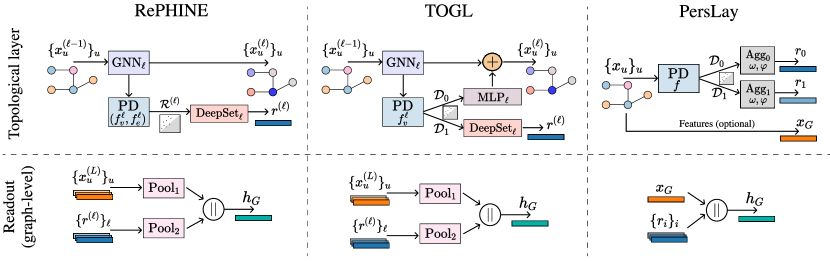
Recently, PH has been used to boost the expressive power of GNNs. Horn et al. (2021) introduce TOGL — a general approach for incorporating topological features from PH into GNN layers. In particular, TOGL leverages node embeddings at each layer of a GNN to obtain vertex-color filtrations. The 0-dim individual persistence tuples are vectorized using MLPs and added to the corresponding node features at each layer. For 1-dim tuples, TOGL applies DeepSets to get a graph-level vector that runs through the final fully-connected layers of the GNN.
Immonen et al. (2023) use independent vertex-color and edge-color filtering functions to obtain more expressive persistent diagrams called RePHINE. More specifically, RePHINE first computes persistence diagrams from a filtration induced by edge colors. Each tuple of the diagram is then augmented based on the vertex colors and the local edge-color information around each vertex. RePHINE diagrams are vectorized using DeepSets and combined with graph-level GNN embeddings in the final classifier. Figure 1 depicts the architectures of RePHINE, TOGL, and PersLay.
-Equivariant networks.
Let be a group acting on two sets and . We say a function is -equivariant if it commutes with the group actions, i.e., for all and , we have that . Here, we are interested in models on geometric simplicial complexes that are equivariant to the Euclidean group , which comprises all translations, rotations, and reflections of the -dim Euclidean space. Eijkelboom et al. (2023) introduce Equivariant Message-Passing Simplicial Networks (EMPSNs), which extends the -equivariant GNNs (Satorras et al., 2021) to geometric simplicial complexes. For each simplex at layer , EMPSNs compute the messages from all , where denotes invariant features (e.g., volumes, angles, distances) computed using coordinates from . Then, the messages to simplex are aggregated using and the same way as in TNNs to obtain an aggregated message . Finally, we recursively update the features and coordinates as
| (4) | ||||
| (5) |
where denotes the upper-adjancency, is a normalization constant, and is an arbitrary function.
Graph ODEs.
Neural Ordinary Differential Equations (ODEs) represent a class of implicit deep learning models characterized by an ODE, where the vector field is parameterized by a neural network (Weinan, 2017; Dupont et al., 2019; Chen et al., 2018; Lu et al., 2018). Graph ODEs (Poli et al., 2019) generalize Neural ODEs to garphs. For instance, we can track the evolution of signals defined over the vertices of a graph as a differential equation
| (6) |
Here, the vector field is parameterized by a neural network. A notable feature is that, under a mild assumption on , employing an Euler scheme for time-steps converges to an -layer Graph ResNet (Sander et al., 2022). This convergence implies that Graph ODEs inherently inherit the capability to incorporate relational inductive biases seen in GNNs while maintaining the dynamic system perspective of continuous-depth models. The versatility of Graph ODEs has paved the way for the design of novel graph neural networks, such as GRAND (Chamberlain et al., 2021), GREAD (Choi et al., 2022), and AbODE (Verma et al., 2023).
3 A unified framework: Topological persistent neural networks (TopNets)
We now introduce a general framework that combines TNNs and PH for expressive learning on topological objects. We call this framework topological persistent neural networks or TopNets, in short. Notably, we show that TopNets subsume several methods at the intersection of PH and GNNs.
To motivate our framework, we show that persistent homology features bring in additional expressive power to TNNs. Bodnar et al. (2021b) introduce a Simplicial Weisfeiler-Leman (SWL) test to characterize the expressivity of simplicial message-passing networks (SMPNs) — a general TNN for simplicial complexes. They show that SWL (with clique complex lifting) is strictly more powerful than 1-WL. Our next result (Proposition 1) implies that the combination of SWL and PH is strictly more expressive than the SWL test.
Proposition 1 (SWL + PH SWL).
There are pairs of non-isomorphic clique complexes that SWL cannot distinguish but persistence diagrams from color-based filtrations can.
Prior works (Horn et al., 2021; Rieck, 2023; Immonen et al., 2023) have demonstrated that PH can be used to increase the power of GNNs. Proposition 1 shows that this also applies to TNNs on simplicial complexes.
Given an input simplicial complex, each layer in a TopNet first applies a general message-passing (MP) procedure to obtain a refined attributed complex, as in TNNs. Then, we compute persistence diagrams followed by a vectorization scheme that assigns each simplex a topological embedding. Next, TopNets obtain two complex-level representations: the first consists of a joint MP-PH vector derived from a combination of the features of the complex and the topological embeddings; and the second one is obtained by merging the PH-based descriptor associated with each simplex via an order-invariant function. Finally, we combine the representation of the simplices at each layer and dimension, and apply two readout layers. The first aims to combine information from different layers (but same dimension) while the second readout function further processes the resulting representations across dimensions. In the following, we formalize these steps.
The final representation in Equation 13 is typically fed through multi-layer perceptrons (MLP) to obtain a complex-level prediction. Importantly, the formalism of TopNets includes PH-based (graph) neural networks such as TOGL (Horn et al., 2021), PersLay (Carrière et al., 2020), and RePHINE (Immonen et al., 2023) as particular cases:
a) TOGL: Here, the functions correspond to GNN layers, while the computation of persistence diagrams () involves vertex-color filtrations, with vectorization achieved via MLPs . The topological aggregation (defined in Appendix C) is specifically applied to persistence tuples of dimension , whose vector representations are added to the initial node features. Tuples of dimension are pooled and then concatenated with the final GNN embedding for use in the subsequent readout phase.
b) PersLay: The serves as an identity transformation, and the computation of the persistence diagram () involves (0-dim and 1-dim) ordinary and extended persistence pairs. Moreover, (defined in Appendix C) simply concatenates node features with graph-level topological vectors.
c) RePHINE: Again, GNN is the choice of TNN. However, the computation of persistence diagrams () involves vertex and edge filtrations specific to RePHINE. The results are aggregated using a DeepSet function to yield a topological embedding for each layer and dimension . The topological aggregation function (defined in Appendix C)outputs the simplex features . Finally, in conjunction with the simplex features from the final layer, the topological embeddings are concatenated and pooled for subsequent use in the downstream readout phase.
More details about deductions can be found in Appendix C.
4 Equivariant TopNets
In this section, we extend TopNets to deal with topological objects that are symmetric to rotation, reflections and translations — i.e., to actions of the Euclidean group . In particular, we consider geometric SCs, and build upon EMPSNs (Eijkelboom et al., 2023) and invariant filtering functions to propose Equivariant TopNets (E-TopNets). Compared to regular TopNets, E-TopNets employ modified general message passing and PH vectorization steps (Eqs. 7 and 8) — the other steps remain untouched.
Starting from an input geometric (attributed) SC ; at each layer , E-TopNets recursively obtain a refined SC via an EMPSN layer as
To achieve an equivariant variant of TopNets, one could disregard the vertex coordinates when computing persistence diagrams. For instance, this can be obtained from an -simplex-color filtration (Definition 1). This generalizes the notion of vertex-color filtrations to higher dimensions. Thus, -simplex-color filtrations are vertex-color ones, -simplex-color filtrations correspond to edge-color filtrations, and so on.
Definition 1 (-simplex-color filtrations).
Let be an attributed simplicial complex and a filtering function. Also, let with . An -simplex-color filtration induced by is a sequence of complexes for , where
Obtaining persistence diagrams from -simplex-color filtrations incurs losing (possibly) relevant geometric information. Thus, here, we are interested in filtering functions that leverage both attributes and coordinates, as in geometric color-based filtrations (Definition 2).
Definition 2 (Geometric -simplex-color filtrations).
Let be a geometric simplicial complex and a filtering function. Also, let with . A geometric -simplex-color filtration induced by is a sequence for , where
and is any - and -invariant function.
For many tasks, e.g., in graph learning, colors are only given to 0-dim simplices. In such cases, we can obtain colors to higher-order simplices via a learnable permutation invariant function on the colors of the vertices in . Thus, we can rewrite the filtering functions in Definition 2 as . As usual, we parameterize using multilayer perceptrons and using DeepSets.
As a remark, persistence diagrams extracted from geometric -simplex-color filtrations are not more expressive than their non-geometric counterparts — i.e., vertex-color (VC) filtrations. The reason is that the only -invariant function of a single element is a constant function, i.e., the condition for all implies that is a constant function. Thus, we refer to their non-geometric variant whenever we mention VC filtrations.
We also note that, to achieve a geometric extension of RePHINE diagrams, we can simply replace its edge-color filtration with a geometric -simplex-color filtration and then use an independent vertex-color function as in the original formulation. This highlights that the vertex coordinates are only used to define filtrations, and any persistence descriptor and vectorization procedure can be applied — having no impact on the equivariance of E-TopNets. Our next result (Proposition 2) establishes the invariance of persistence diagrams from geometric -simplex-color filtrations.
Proposition 2 (Invariant persistence diagrams).
For any , persistence diagrams for any dimension obtained from geometric -simplex-color filtrations are -invariant.
We can rewrite the PH vectorization step of E-TopNets as
where denotes one or more -invariant filtering functions used to induce a geometric -simplex-color filtration for some in .
5 Continuous (Equivariant) TopNets
In this section, we expand the general framework of (Equivariant) TopNets to encompass continuous systems. Unlike conventional E-TopNets, Continuous E-TopNets use a continuous message-passing scheme based on EMPSNs. For each simplex at time-step , we compute the messages from all . Then, the messages to simplex are aggregated using and the same way as in TNNs to obtain an aggregated message . Finally, we apply the following functions to obtain the refined feature vectors as
| (14) | ||||
| (15) |
where is a constant and is an arbitrary non-linear mapping. The forward solution of can be accurately approximated with numerical solvers such as RK4 (Runge, 1895) with low computational cost. The geometrical filtrations and topological embeddings are computed in the same way as described in the previous section.
Interestingly, one can define a set of associated Neural ODEs for a given PH-based (graph) neural network such as TOGL and RePHINE. We derive the set of neural ODEs and utilize it to derive discretization error bounds between discrete and continuous trajectories.
| TNN | Topological Agg | Diagram | Method | NCI109 | IMDB-B | NCI1 | MOLHIV | PROTEINS |
| GCN | VC | Discrete | 77.92 1.03 | 64.80 1.30 | 79.08 1.06 | 73.64 1.29 | 69.46 1.83 | |
| Continuous | 80.37 2.21 | 73.40 3.40 | 81.75 2.93 | 72.41 3.29 | 72.892.10 | |||
| RePHINE | Discrete | 79.18 1.97 | 69.40 3.78 | 80.44 0.94 | 75.98 1.80 | 71.25 1.60 | ||
| Continuous | 80.63 1.56 | 76.00 2.10 | 82.15 1.75 | 74.90 2.78 | 73.79 1.30 | |||
| GIN | VC | Discrete | 78.35 0.68 | 69.80 0.84 | 79.12 1.23 | 73.37 4.36 | 69.46 2.48 | |
| Continuous | 80.391.13 | 74.00 3.25 | 82.18 1.56 | 71.90 5.20 | 72.89 2.15 | |||
| RePHINE | Discrete | 79.23 1.67 | 72.80 2.95 | 80.92 1.92 | 73.71 0.91 | 72.32 1.89 | ||
| Continuous | 81.60 0.95 | 76.00 1.60 | 84.16 1.89 | 72.10 4.27 | 73.79 1.45 | |||
| MPSN | VC | Discrete | 79.40 2.74 | 66.50 3.65 | 77.10 1.37 | 72.40 3.90 | 70.50 1.75 | |
| Continuous | 80.10 3.45 | 73.00 1.80 | 81.10 4.64 | 72.70 4.65 | 71.20 3.20 | |||
| RePHINE | Discrete | 79.43 1.65 | 67.20 2.85 | 81.22 1.48 | 71.20 4.78 | 71.70 2.56 | ||
| Continuous | 80.40 3.55 | 74.00 2.65 | 83.20 3.24 | 71.50 4.54 | 72.10 2.35 |
5.1 Discretization Error Bound
We compute discretization error bounds between the trajectories for discrete and continuous versions of RePHINE and TOGL. All the proofs can be found in Appendix E.
Proposition 3 (Discretization error for TOGL).
The discretization error for node at layer between the node features of -layer (with time-step size ) continuous and discrete TOGL networks is bounded as
| (16) |
where and are Lipshitz constants, and is a remainder term associated with the Taylor expansion of continuous TOGL.
Proposition 4 (Discretization error for RePHINE).
Let and be the node and topological embeddings of an -time-step continuous RePHINE model at time-step , respectively. Similarly, let and be the node and topological embeddings of a discrete -layer RePHINE at layer . Then, we can bound the discretization errors and as follows:
| (17) | ||||
| (18) | ||||
where are Lipshitz constants, and are the remainder terms associated with the Taylor expansion of continuous RePHINE.
| Model | Diagram | Enzymes | DD | Proteins |
| GCN | - | 65.8 4.6 | 72.8 4.1 | 76.1 2.4 |
| TOGL | VC | 53.0 9.2 | 73.2 4.7 | 76.0 3.9 |
| Cont. TopNets | 69.7 3.2 | 73.1 1.9 | 78.7 2.7 | |
| GIN | - | 50.0 12.3 | 70.8 3.8 | 72.3 3.3 |
| TOGL | VC | 43.8 7.9 | 75.2 4.2 | 73.6 4.8 |
| Cont. TopNets | 58.3 8.2 | 77.3 4.5 | 79.5 3.9 |
Implication. The bound indicates that the proximity to the ODE solution cannot be assured since it is uncertain whether . This suggests the necessity of incorporating additional regulatory assumptions over the network to obtain the Neural ODE in the large depth limit. This observation resonates closely with the analysis conducted by Sander et al. (2022) in characterizing Neural ODEs with ResNets.
6 Experiments
| Architecture | Diagram | Method | ZPVE | |||||||
| meV | meV | meV | D | cal/mol K | meV | |||||
| DimeNet | - | - | 0.044 | 33 | 25 | 20 | 0.030 | 0.023 | 0.331 | 1.21 |
| SphereNet△ | - | - | 0.046 | 32 | 23 | 18 | 0.026 | 0.021 | 0.292 | 1.21 |
| NMP | - | - | 0.092 | 69 | 43 | 38 | 0.030 | 0.040 | 0.180 | 1.50 |
| -Tr | - | - | 0.142 | 53 | 35 | 33 | 0.051 | 0.054 | - | - |
| TFN | - | - | 0.223 | 58 | 40 | 38 | 0.064 | 0.101 | - | - |
| MPSN | - | - | 0.266 | 153 | 89 | 77 | 0.101 | 0.122 | 0.887 | 3.02 |
| EGNN | - | - | 0.071 | 48 | 29 | 25 | 0.028 | 0.031 | 0.106 | 1.55 |
| IMPSN∗∗ | - | - | 0.066 | 51 | 32 | 25 | 0.031 | 0.027 | 0.114 | 1.44 |
| IMPSN | VC | Disc. E-TopNets | 0.083 | 47 | 37 | 24 | 0.035 | 0.032 | 0.125 | 1.45 |
| Cont. E-TopNets | 0.075 | 49 | 36 | 27 | 0.030 | 0.035 | 0.129 | 1.43 | ||
| RePHINE | Disc. E-TopNets | 0.072 | 57 | 33 | 28 | 0.029 | 0.028 | 0.132 | 1.39 | |
| Cont. E-TopNets | 0.070 | 50 | 35 | 25 | 0.032 | 0.030 | 0.118 | 1.37 |
Tasks. We assess the performance of TopNets on diverse tasks: (i) we evaluate our method performance on real-world graph classification data while considering discrete and continuous versions of various GNNs and TNNs in Section 6.1, (ii) we benchmark TopNets efficacy in property prediction using QM9 molecular data, highlighting the effectiveness of its equivariant variant in Section 6.2, (iii) we demonstrate TopNets utility in co-designing antibody sequence and structure using the SAbDab database in Section 6.3, and (iv) we evaluate our method on 3BPA MD17 trajectories (Kovács et al., 2021) in Section 6.4.
Baselines. On graph classification tasks, we use standard vertex-color (VC) and RePHINE (Immonen et al., 2023) to compute persistence diagrams. We adopt different GNN/TNN architectures like GCN (Kipf and Welling, 2016), GIN (Xu et al., 2019), TOGL (Horn et al., 2021), and MPSN (Bodnar et al., 2021a). We also compare the performance between each method’s continuous and discrete counterparts. On QM9 property prediction tasks, we compare TopNets to several equivariant methods like NMP (Gilmer et al., 2017), TFN (Thomas et al., 2018), -Tr (Fuchs et al., 2020), DimeNet++ (Gasteiger et al., 2020a), SphereNet (Liu et al., 2021), MPSN(Bodnar et al., 2021a), EGNN (Satorras et al., 2021) and IMPSN (Eijkelboom et al., 2023). On CDR-H3 Antibody design, we compare to recent SOTA like RefineGNN (Jin et al., 2022), MEAN (Kong et al., 2023) and AbODE (Verma et al., 2023). Lastly, for 3BPA MD17 trajectories, we compare our method to SOTA like NequIP (Batzner et al., 2022) and MACE (Batatia et al., 2022) which use higher-order message passing mechanisms.
Implementation details are given in Appendix B.
6.1 Graph Classification
The results presented in Table 2 and Table 3 demonstrate the performance of TopNets on graph classification. These results offer a detailed assessment of different GNN/TNN architectures, PH vectorization methods, and their continuous counterparts. The reported results include the mean and standard deviation of predictive metrics — AUROC for MOLHIV and accuracy for the remaining datasets. This comprehensive analysis provides valuable insights into TopNets performance. Notably, incorporating the continuous component consistently improves downstream performance across all datasets, TNNs, and schemes.
6.2 Molecular data - QM9
The QM9 dataset, introduced by Ramakrishnan et al. (2014), comprises small molecules with a maximum of 29 atoms in 3D space. Each atom is characterized by a 3D position and a five-dimensional one-hot node embedding representing the atom type, denoted as . The dataset’s primary objective is to predict various chemical properties of the molecules, which remain invariant to translations, rotations, and reflections on the atom positions. Following the data preparation strategy of Eijkelboom et al. (2023); Satorras et al. (2021), we partition the dataset into training, validation, and test sets. The mean absolute error between predictions and ground truth for test set is reported in Table 4, revealing the competitive performance of TopNets compared to baselines. Notably, on many targets, TopNets achieve results nearly on par with SOTA approaches, surpassing in predicting ZPVE, and . This achievement is intriguing as our architecture, not specifically tailored for molecular tasks, lacks many molecule-specific intricacies, like Bessel function embeddings (Gasteiger et al., 2020b).
6.3 CDR-H3 Antibody Design
We took the antigen-antibody complexes dataset from Structural Antibody Database (Dunbar et al., 2014) and removed invalid data points. We followed a strategy similar to Verma et al. (2023) for data preparation and splitting and employ Amino Acid Recovery (AAR) and RMSD for quantitative evaluation. AAR is defined as the overlapping rate between the predicted 1D sequences and the ground truth. RMSD is calculated via the Kabsch algorithm (Kabsch, 1976) based on spatial features of the CDR residues.
| Method | Diagram | AAR () | RMSD () |
| LSTM | - | 15.69 0.91 | (N/A) |
| C-LSTM | - | 15.48 1.17 | (N/A) |
| RefineGNN | - | 21.13 1.59 | 6.00 0.55 |
| C-RefineGNN | - | 18.88 1.37 | 6.22 0.59 |
| MEAN | - | 36.38 3.08 | 2.21 0.16 |
| AbODE | - | 39.8 1.17 | 1.73 0.11 |
| TopNets | VC | 43.00 1.34 | 1.73 0.21 |
| RePHINE | 44.80 1.57 | 1.75 0.17 |
Table 5 showcases the performance of TopNets compared to the baseline methods over CDR-H3 design. TopNets outperform other methods in terms of sequence prediction, thus improving over the SOTA and demonstrating the benefit of persistent homology in generative design.
6.4 Molecular Dynamics
We use the standard 3BPA MD17 (Kovács et al., 2021) dataset to evaluate the extrapolation capabilities. The training set consists of geometries sampled from K molecular dynamics simulation of the large and flexible drug-like molecule 3-(benzyloxy)pyridin-2-amine. The three test sets contain geometries sampled at 300 K, 600 K, and 1200 K to assess in- and out-of-domain accuracy. The task is to predict the (E, meV) and force (F, meV/) of the given conformations. In order to have a fair comparison, we followed the same data-preparation strategy and training setup as described in Batatia et al. (2022).
| Task | Variable | NequIP | MACE | TopNets |
| 300K | E | 3.30.1 | 3.00.2 | 2.50.2 |
| F | 10.80.2 | 8.80.3 | 8.9 0.2 | |
| 600K | E | 11.20.1 | 9.70.5 | 9.50.7 |
| F | 26.40.1 | 21.80.6 | 21.8 0.7 | |
| 1200K | E | 38.51.6 | 29.81.0 | 29.21.2 |
| F | 76.21.1 | 62.0 1.8 | 62.3 0.5 |
Table 6 showcases the performance of TopNets compared to the baseline methods over energy (E, meV) and force (F, meV/) on different sets of geometries sampled at 300 K, 600 K, and 1200 K. We used to aggregate and compute the PH embeddings. Notably, our results indicate that TopNets and MACE generally outperform NequIP in predicting energy as well as force of the molecular configurations.
7 Ablations
Runtime comparison. We conducted an ablation study to characterize the runtime complexity of our method, assessing the time taken per epoch to train different models on a single V100 GPU. The results are shown in Table 7, and as expected, continuous methods require additional time due to solving the ODE forward compared to their discrete counterparts. However, the ODE-based methods can be trained without storing intermediate quantities, leading to a constant memory requirement (Chen et al., 2018) as compared to the memory cost of training other methods which increases with the depth of the network.
Higher-order PH. We conducted an ablation study to evaluate the influence of higher-order persistent homology (PH) features on TNNs. We employed fixed filtering functions based on curvature filtrations (Southern et al., 2024) to extract level diagrams corresponding to -dim topological features. These features are then aggregated using deepsets (Zaheer et al., 2017) to combine with pooled node features extracted by the TNN for downstream tasks. We evaluate the method on two graph classification datasets: IMDB-Binary and Proteins — we apply uplifting to obtain clique complexes from which we extract persistence diagrams (Southern et al., 2024). The results shown in Table 8 demonstrate that incorporating higher-order PH features leads to improved performance across various TNNs on both datasets.
| TNN | Diagram | Method | Time (GPU time) |
| GCN | VC | Discrete | 62.9 11.5 |
| Continuous | 106.8 12.8 | ||
| RePHINE | Discrete | 62.7 13.4 | |
| Continuous | 112.7 16.7 | ||
| GIN | VC | Discrete | 60.7 8.7 |
| Continuous | 105.7 10.8 | ||
| RePHINE | Discrete | 65.9 10.5 | |
| Continuous | 120.7 15.7 |
| TNN | IMDB-B | Proteins |
| GCN | 73.0 1.30 | 71.4 1.10 |
| GIN | 76.0 1.70 | 74.2 2.10 |
| MPSN | 76.0 1.50 | 74.5 2.75 |
8 Conclusion and Limitations
We introduce TopNets to illustrate the theoretical and practical benefits of including persistent features in topological networks, and their geometric and continuous-time extensions. TopNets incur considerable computational expense due to costs involved in computing PH embeddings as well as higher-order message-passing. Additionally, our research is confined to simplicial complexes, and exploring combinatorial complexes is an interesting avenue for future work.
Acknowledgements
This work has been supported by the Research Council of Finland under the HEALED project (grant 13342077), Jane and Aatos Erkko Foundation project (grant 7001703) on “Biodesign: Use of artificial intelligence in enzyme design for synthetic biology”, and Finnish Center for Artificial Intelligence FCAI (Flagship programme). We acknowledge CSC – IT Center for Science, Finland, for providing generous computational resources.
Impact Statement
We proposed a framework for topological representation learning, leveraging persistent homology and topological neural networks. Our contributions advance current art by offering a unified framework for topological deep learning, and extending it to accommodate geometric features naturally appearing in many downstream real-world applications. Potential applications in drug property prediction, molecular simulation, and protein generative design have significant implications for drug development and precision medicine.
References
- Adams et al. (2016) Henry Adams, Tegan Emerson, Michael Kirby, Rachel Neville, Chris Peterson, Patrick Shipman, Sofya Chepushtanova, Eric Hanson, Francis Motta, and Lori Ziegelmeier. Persistence Images: A Stable Vector Representation of Persistent Homology. Journal of Machine Learning Research, 18(8):1–35, 2016.
- Barbarossa and Sardellitti (2020) Sergio Barbarossa and Stefania Sardellitti. Topological signal processing over simplicial complexes. IEEE Transactions on Signal Processing, 68:2992–3007, 2020.
- Batatia et al. (2022) Ilyes Batatia, David P Kovacs, Gregor Simm, Christoph Ortner, and Gábor Csányi. Mace: Higher order equivariant message passing neural networks for fast and accurate force fields. Advances in Neural Information Processing Systems, 35:11423–11436, 2022.
- Batzner et al. (2022) Simon Batzner, Albert Musaelian, Lixin Sun, Mario Geiger, Jonathan P. Mailoa, Mordechai Kornbluth, Nicola Molinari, Tess E. Smidt, and Boris Kozinsky. E(3)-equivariant graph neural networks for data-efficient and accurate interatomic potentials. Nature Communications, 13(1), May 2022. ISSN 2041-1723. doi: 10.1038/s41467-022-29939-5.
- Bodnar et al. (2021a) Cristian Bodnar, Fabrizio Frasca, Nina Otter, Yuguang Wang, Pietro Liò, Guido F Montufar, and Michael Bronstein. Weisfeiler and lehman go cellular: Cw networks. In Advances in Neural Information Processing Systems (NeurIPS), 2021a.
- Bodnar et al. (2021b) Cristian Bodnar, Fabrizio Frasca, Yuguang Wang, Nina Otter, Guido F Montufar, Pietro Lio, and Michael Bronstein. Weisfeiler and lehman go topological: Message passing simplicial networks. In International Conference on Machine Learning (ICML), 2021b.
- Brandstetter et al. (2023) Johannes Brandstetter, Rianne van den Berg, Max Welling, and Jayesh Gupta. Clifford neural layers for PDE modeling. In ICLR, 2023.
- Brehmer et al. (2023) Johann Brehmer, Pim De Haan, Sönke Behrends, and Taco Cohen. Geometric algebra transformers. arXiv preprint arXiv:2305.18415, 2023.
- Bronstein et al. (2021) Michael M. Bronstein, Joan Bruna, Taco Cohen, and Petar Velicković. Geometric deep learning: Grids, groups, graphs, geodesics, and gauges, 2021.
- Bubenik (2015) P. Bubenik. Statistical topological data analysis using persistence landscapes. Journal of Machine Learning Research, 16:77–102, 2015.
- Carrière et al. (2020) Mathieu Carrière, Frédéric Chazal, Yuichi Ike, Théo Lacombe, Martin Royer, and Yuhei Umeda. PersLay: A Neural Network Layer for Persistence Diagrams and New Graph Topological Signatures. In Artificial Intelligence and Statistics (AISTATS), 2020.
- Chamberlain et al. (2021) Ben Chamberlain, James Rowbottom, Maria I Gorinova, Michael Bronstein, Stefan Webb, and Emanuele Rossi. Grand: Graph neural diffusion. In International Conference on Machine Learning, pages 1407–1418. PMLR, 2021.
- Chen et al. (2019) Binghui Chen, Weihong Deng, and Jiani Hu. Mixed high-order attention network for person re-identification. In Proceedings of the IEEE/CVF international conference on computer vision, pages 371–381, 2019.
- Chen et al. (2018) Ricky T. Q. Chen, Yulia Rubanova, Jesse Bettencourt, and David K Duvenaud. Neural ordinary differential equations. In S. Bengio, H. Wallach, H. Larochelle, K. Grauman, N. Cesa-Bianchi, and R. Garnett, editors, Advances in Neural Information Processing Systems, volume 31. Curran Associates, Inc., 2018.
- Choi et al. (2022) Jeongwhan Choi, Seoyoung Hong, Noseong Park, and Sung-Bae Cho. Gread: Graph neural reaction-diffusion equations. arXiv preprint arXiv:2211.14208, 2022.
- Demailly (2006) Jean-Pierre Demailly. Analyse numérique et équations différentielles. EDP sciences Les Ulis, 2006.
- Dong et al. (2020) Yihe Dong, Will Sawin, and Yoshua Bengio. Hnhn: Hypergraph networks with hyperedge neurons. arXiv preprint arXiv:2006.12278, 2020.
- Dunbar et al. (2014) James Dunbar, Konrad Krawczyk, Jinwoo Leem, Terry Baker, Angelika Fuchs, Guy Georges, Jiye Shi, and Charlotte M Deane. Sabdab: the structural antibody database. Nucleic acids research, 42(D1):D1140–D1146, 2014.
- Dupont et al. (2019) Emilien Dupont, Arnaud Doucet, and Yee Whye Teh. Augmented neural odes. Advances in neural information processing systems, 32, 2019.
- Duval et al. (2023) Alexandre Duval, Simon V. Mathis, Chaitanya K. Joshi, Victor Schmidt, Santiago Miret, Fragkiskos D. Malliaros, Taco Cohen, Pietro Lio, Yoshua Bengio, and Michael Bronstein. A hitchhiker’s guide to geometric gnns for 3d atomic systems, 2023.
- Edelsbrunner and Harer (2010) H. Edelsbrunner and J. Harer. Computational Topology - an Introduction. American Mathematical Society, 2010.
- Eijkelboom et al. (2023) Floor Eijkelboom, Rob Hesselink, and Erik Bekkers. E(n) equivariant message passing simplicial networks. arXiv preprint arXiv:2305.07100, 2023.
- Freeman (2004) Linton Freeman. The development of social network analysis. A Study in the Sociology of Science, 1(687):159–167, 2004.
- Fuchs et al. (2020) Fabian Fuchs, Daniel Worrall, Volker Fischer, and Max Welling. Se (3)-transformers: 3d roto-translation equivariant attention networks. Advances in neural information processing systems, 33:1970–1981, 2020.
- Garg et al. (2020) Vikas K. Garg, Stefanie Jegelka, and Tommi Jaakkola. Generalization and representational limits of graph neural networks. In International Conference on Machine Learning, 2020.
- Gasteiger et al. (2020a) Johannes Gasteiger, Shankari Giri, Johannes T Margraf, and Stephan Günnemann. Fast and uncertainty-aware directional message passing for non-equilibrium molecules. arXiv preprint arXiv:2011.14115, 2020a.
- Gasteiger et al. (2020b) Johannes Gasteiger, Janek Groß, and Stephan Günnemann. Directional message passing for molecular graphs. arXiv preprint arXiv:2003.03123, 2020b.
- Geiger and Smidt (2022) Mario Geiger and Tess Smidt. e3nn: Euclidean neural networks. arXiv preprint arXiv:2207.09453, 2022.
- Gilmer et al. (2017) Justin Gilmer, Samuel S Schoenholz, Patrick F Riley, Oriol Vinyals, and George E Dahl. Neural message passing for quantum chemistry. In International conference on machine learning, pages 1263–1272. PMLR, 2017.
- Giusti et al. (2023) Lorenzo Giusti, Claudio Battiloro, Lucia Testa, Paolo Di Lorenzo, Stefania Sardellitti, and Sergio Barbarossa. Cell attention networks. In 2023 International Joint Conference on Neural Networks (IJCNN), pages 1–8. IEEE, 2023.
- Grathwohl et al. (2018) Will Grathwohl, Ricky TQ Chen, Jesse Bettencourt, Ilya Sutskever, and David Duvenaud. Ffjord: Free-form continuous dynamics for scalable reversible generative models. arXiv preprint arXiv:1810.01367, 2018.
- Hensel et al. (2021) Felix Hensel, Michael Moor, and Bastian Rieck. A survey of topological machine learning methods. Frontiers in Artificial Intelligence, 4, 2021.
- Hofer et al. (2017) C. Hofer, R. Kwitt, M. Niethammer, and A. Uhl. Deep learning with topological signatures. In Advances in Neural Information Processing Systems (NeurIPS), 2017.
- Horn et al. (2021) Max Horn, Edward De Brouwer, Michael Moor, Yves Moreau, Bastian Rieck, and Karsten Borgwardt. Topological graph neural networks. arXiv preprint arXiv:2102.07835, 2021.
- Iakovlev et al. (2020) Valerii Iakovlev, Markus Heinonen, and Harri Lähdesmäki. Learning continuous-time pdes from sparse data with graph neural networks. arXiv preprint arXiv:2006.08956, 2020.
- Immonen et al. (2023) Johanna Immonen, Amauri H. Souza, and Vikas Garg. Going beyond persistent homology using persistent homology. In Advances in Neural Information Processing Systems (NeurIPS), 2023.
- Jha et al. (2022) Kanchan Jha, Sriparna Saha, and Hiteshi Singh. Prediction of protein–protein interaction using graph neural networks. Scientific Reports, 12(1):8360, 2022.
- Jin et al. (2022) Wengong Jin, Jeremy Wohlwend, Regina Barzilay, and Tommi Jaakkola. Iterative refinement graph neural network for antibody sequence-structure co-design, 2022.
- Joshi et al. (2023) Chaitanya K. Joshi, Cristian Bodnar, Simon V. Mathis, Taco Cohen, and Pietro Liò. On the expressive power of geometric graph neural networks, 2023.
- Kabsch (1976) Wolfgang Kabsch. A solution for the best rotation to relate two sets of vectors. Acta Crystallographica Section A: Crystal Physics, Diffraction, Theoretical and General Crystallography, 32(5):922–923, 1976.
- Kim et al. (2023) Timothy Doyeon Kim, Tankut Can, and Kamesh Krishnamurthy. Trainability, expressivity and interpretability in gated neural odes. arXiv preprint arXiv:2307.06398, 2023.
- Kipf and Welling (2016) Thomas N Kipf and Max Welling. Semi-supervised classification with graph convolutional networks. arXiv preprint arXiv:1609.02907, 2016.
- Kochkov et al. (2021) Dmitrii Kochkov, Jamie Smith, Ayya Alieva, Qing Wang, Michael Brenner, and Stephan Hoyer. Machine learning–accelerated computational fluid dynamics. Proceedings of the National Academy of Sciences, 118(21), 2021.
- Kong et al. (2023) Xiangzhe Kong, Wenbing Huang, and Yang Liu. Conditional antibody design as 3d equivariant graph translation, 2023.
- Kovács et al. (2021) Dávid Péter Kovács, Cas van der Oord, Jiri Kucera, Alice EA Allen, Daniel J Cole, Christoph Ortner, and Gábor Csányi. Linear atomic cluster expansion force fields for organic molecules: beyond rmse. Journal of chemical theory and computation, 17(12):7696–7711, 2021.
- Kusano et al. (2016) Genki Kusano, Yasuaki Hiraoka, and Kenji Fukumizu. Persistence weighted Gaussian kernel for topological data analysis. In International Conference on Machine Learning (ICML), pages 2004–2013, 2016.
- Li et al. (2021) Zongyi Li, Nikola Kovachki, Kamyar Azizzadenesheli, Burigede Liu, Kaushik Bhattacharya, Andrew Stuart, and Anima Anandkumar. Fourier neural operator for parametric partial differential equations. In ICLR, 2021.
- Lipman et al. (2023) Yaron Lipman, Ricky T. Q. Chen, Heli Ben-Hamu, Maximilian Nickel, and Matt Le. Flow matching for generative modeling, 2023.
- Liu et al. (2021) Yi Liu, Limei Wang, Meng Liu, Xuan Zhang, Bora Oztekin, and Shuiwang Ji. Spherical message passing for 3d graph networks. arXiv preprint arXiv:2102.05013, 2021.
- Lu et al. (2021) Lu Lu, Pengzhan Jin, Guofei Pang, Zhongqiang Zhang, and George Em Karniadakis. Learning nonlinear operators via DeepONet based on the universal approximation theorem of operators. Nature machine intelligence, 3(3):218–229, 2021.
- Lu et al. (2018) Yiping Lu, Aoxiao Zhong, Quanzheng Li, and Bin Dong. Beyond finite layer neural networks: Bridging deep architectures and numerical differential equations. In International Conference on Machine Learning, pages 3276–3285. PMLR, 2018.
- Marion (2023) Pierre Marion. Generalization bounds for neural ordinary differential equations and deep residual networks. arXiv preprint arXiv:2305.06648, 2023.
- Papillon et al. (2023) Mathilde Papillon, Sophia Sanborn, Mustafa Hajij, and Nina Miolane. Architectures of topological deep learning: A survey on topological neural networks. ArXiv e-prints, 2023.
- Poli et al. (2019) Michael Poli, Stefano Massaroli, Junyoung Park, Atsushi Yamashita, Hajime Asama, and Jinkyoo Park. Graph neural ordinary differential equations. arXiv preprint arXiv:1911.07532, 2019.
- Ramakrishnan et al. (2014) Raghunathan Ramakrishnan, Pavlo O Dral, Matthias Rupp, and O Anatole Von Lilienfeld. Quantum chemistry structures and properties of 134 kilo molecules. Scientific data, 1(1):1–7, 2014.
- Rieck (2023) B. Rieck. On the expressivity of persistent homology in graph learning. arXiv: 2302.09826, 2023.
- Runge (1895) Carl Runge. Über die numerische auflösung von differentialgleichungen. Mathematische Annalen, 46(2):167–178, 1895.
- Sander et al. (2022) Michael Sander, Pierre Ablin, and Gabriel Peyré. Do residual neural networks discretize neural ordinary differential equations? Advances in Neural Information Processing Systems, 35:36520–36532, 2022.
- Satorras et al. (2021) Vıctor Garcia Satorras, Emiel Hoogeboom, and Max Welling. E (n) equivariant graph neural networks. In International conference on machine learning, pages 9323–9332. PMLR, 2021.
- Shi et al. (2020) Yunsheng Shi, Zhengjie Huang, Shikun Feng, Hui Zhong, Wenjin Wang, and Yu Sun. Masked label prediction: Unified message passing model for semi-supervised classification. arXiv preprint arXiv:2009.03509, 2020.
- Southern et al. (2024) Joshua Southern, Jeremy Wayland, Michael Bronstein, and Bastian Rieck. Curvature filtrations for graph generative model evaluation. Advances in Neural Information Processing Systems, 36, 2024.
- Thomas et al. (2018) Nathaniel Thomas, Tess Smidt, Steven Kearnes, Lusann Yang, Li Li, Kai Kohlhoff, and Patrick Riley. Tensor field networks: Rotation-and translation-equivariant neural networks for 3d point clouds. arXiv preprint arXiv:1802.08219, 2018.
- Thorpe et al. (2022) Matthew Thorpe, Tan Minh Nguyen, Heidi Xia, Thomas Strohmer, Andrea Bertozzi, Stanley Osher, and Bao Wang. Grand++: Graph neural diffusion with a source term. In International Conference on Learning Representation (ICLR), 2022.
- Velicković et al. (2017) Petar Velicković, Guillem Cucurull, Arantxa Casanova, Adriana Romero, Pietro Lio, and Yoshua Bengio. Graph attention networks. arXiv preprint arXiv:1710.10903, 2017.
- Verma et al. (2022) Yogesh Verma, Samuel Kaski, Markus Heinonen, and Vikas Garg. Modular flows: Differential molecular generation. arXiv preprint arXiv:2210.06032, 2022.
- Verma et al. (2023) Yogesh Verma, Markus Heinonen, and Vikas Garg. AbODE: Ab initio antibody design using conjoined ODEs. In Proceedings of the 40th International Conference on Machine Learning, pages 35037–35050. PMLR, 2023.
- Verma et al. (2024) Yogesh Verma, Markus Heinonen, and Vikas Garg. ClimODE: Climate and weather forecasting with physics-informed neural ODEs. In The Twelfth International Conference on Learning Representations, 2024.
- Weinan (2017) Ee Weinan. A proposal on machine learning via dynamical systems. Communications in Mathematics and Statistics, 1(5):1–11, 2017.
- Weisfeiler and Leman (1968) Boris Weisfeiler and Andrei Leman. The reduction of a graph to canonical form and the algebra which appears therein. nti, Series, 2(9):12–16, 1968.
- Xu et al. (2019) K. Xu, W. Hu, J. Leskovec, and S. Jegelka. How powerful are graph neural networks? In International Conference on Learning Representations (ICLR), 2019.
- Yildiz et al. (2019) Cagatay Yildiz, Markus Heinonen, and Harri Lahdesmaki. ODE2VAE: Deep generative second order ODEs with Bayesian neural networks. NeurIPS, 2019.
- Zaheer et al. (2017) Manzil Zaheer, Satwik Kottur, Siamak Ravanbakhsh, Barnabas Poczos, Russ R Salakhutdinov, and Alexander J Smola. Deep sets. In Advances in Neural Information Processing Systems (NeurIPS), volume 30, 2017.
Appendix A Persistent homology
Persistent homology (PH) stands as a cornerstone in topological data analysis (TDA). At its core, PH seeks to capture multiresolution topological features (e.g., connected components, loops, voids, etc.) from data. Here, we offer a short overview of PH and direct readers to [Hensel et al., 2021] and [Edelsbrunner and Harer, 2010] for an exhaustive treatment.
In the following, we consider topological spaces given by simplicial complexes. In particular, consider a simplicial complex denoted by . The -chains are formal sums , where and represent -dimensional simplices in . By equipping -chains with addition, we obtain the group . Another important notion is that of boundary of a simplex. Consider a -simplex . The boundary of corresponds to the sum of its -dimensional faces, i.e.,
Importantly, we can extend this definition to define the boundary homomorphism , where . Then, we can define a sequence of groups, also called a chain complex, as:
where groups are connected via boundary homomorphisms. The -th homology group comprises -chains with empty boundaries (i.e., ), whereby each of these specific -chains (cycles) represents a boundary of a distinct simplex in . Hence, we define the -th homology group as the quotient space:
The -th Betti number of , denoted by , is equal to the rank of .
In persistent homology, we keep track of the evolution of Betti numbers across a sequence of chain complexes. The sequence of complexes arise from a filtration — a nested sequence of simplicial subcomplexes , indexed by timestamps (with for all ). By computing the homology groups for each of these simplicial complexes, we obtain detailed topological information from . In practice, this is done by associating a pair of timestamps for every element of the homology groups (or topological features), indicating the filtration timestamp at which it emerged and disappeared. The persistence of a point denotes the duration for which the corresponding feature persisted. We set if the topological feature persists until the final filtration timestamp. Formally, let and be the standard -cycle and -boundary groups for the complex . Then, the th persistent homology groups are
for all . Again, the -th persistent Betti number corresponds to the rank of . Finally, a persistence diagram comprising the persistence pairs with corresponding multiplicities given by encodes the persistent homology groups.
Appendix B Implementation Details
Below are the implementation details.
B.1 Graph Classification
We followed the following hyperparameters and training setup in Table 9 to conduct our experiments on real-world graph classification.
| Hyperparameter | Meaning | Value |
| Solver | ODE-Solver | adaptive-heun,euler |
| GNN | GNN Architecture | {GCN,GIN,MPSN} |
| PH | Type of PH | {VC,TOGL,RePHINE} |
| Steps | Number of steps for ODE solver | {20,15,10,5} |
| Node Hidden Dim | Latent dimension of node features | 128 |
| PH embed dim | Latent dimension of PH features | 64 |
| Num Filt | Number of filtrations | 8 |
| Hiden Filtration | Hidden dimension of filtration functions | 16 |
| Batch Size | Size of batches | 64 |
| LR | Learning Rate | 0.001 |
| Scheduler | Learning Rate scheduler | Cosine-Annealing-LR |
| Epochs | Number of epochs | 300 |
B.2 Molecular Data QM9
For the discrete case, we followed the data-preparation strategies, training setup, and hyperparameters as outlined by Eijkelboom et al. [2023]. We enhanced each layer with an Equivariant RePHINE layer, inspired by the original RePHINE [Immonen et al., 2023], incorporating Euclidean distance as an invariant feature in the filtration function. The Vertex Cloud (VC) retained its absence of 3D positional information, consistent with [Immonen et al., 2023]. For the continuous case, we employed a single layer of EMPSN to parameterize the ODE dynamics, leveraging the odeint package to solve these dynamics. Additionally, an Equivariant RePHINE layer was applied per time step. Solver options included euler and adaptive-heun, with the number of time steps ranging from 5 to 20. Filtration parameters remained consistent with those described in Table 9, alongside identical training hyperparameters and setup as in the original EPMSN paper.
B.3 CDR-H3 Antibody Design
We followed the following hyperparameters to conduct our experiments on CDR-H3 Antibody Design.
| Hyperparameter | Meaning | Value |
| GNN | GNN Architecture | TransformerConv [Shi et al., 2020] |
| PH | Type of PH | {VC,RePHINE} |
| Layers | Number of layers | 4 |
| Node Hidden Dim | Latent dimension of node features | [128,256,128,64] |
| PH embed dim | Latent dimension of PH features | 64 |
| Num Filt | Number of filtrations | 8 |
| Hiden Filtration | Hidden dimension of filtration functions | 16 |
| Batch Size | Size of batches | 32 |
| LR | Learning Rate | 0.001 |
| Scheduler | Learning Rate scheduler | Cosine-Annealing-LR |
| Epochs | Number of epochs | 1000 |
Appendix C Deduction from TopNets
In our study we restrict ourselves to -dim simplicial complexes (otherwise mentioned) and here we showcases the deductions of various methods from TopNets.
The readout layers for TOGL concatenate the aggregated topological embeddings (-dim ) with the last layer pooled -dim simplex features and using it for downstream tasks such as classification.
In case of PersLay, they does not use any TNN layers over the node features, thus are N/A, and the other aggregation is performed as,
However PersLay, utilizes an additional option to use the pooled -dim simplex features via concatenating it with the aggregated topological embeddings (-dim and -dim) and using it for downstream tasks such as classification.
The readout layers for RePHINE concatenate the aggregated topological embeddings (-dim and -dim) with the last layer pooled -dim simplex features and using it for downstream tasks such as classification.
Note that wherever we utilise as the topological aggregation method we utilise their specific readout layers as well. The Table 11 summarizes the deduction further from TopNets for various methods.
| Module | Meaning | TOGL | PersLay | RePHINE |
| TNN/GNN Architecture | {GCN,GIN} | - | {GCN,GIN} | |
| Type of PH-diagrams used | VC | VC, Point transformations | RePHINE | |
| Filtration functions | ||||
| Diagram combining functions | DeepSets | DeepSets | DeepSets | |
| Topological Aggregation |
Appendix D Proofs
D.1 Proof of Proposition 1
Let us first introduce two important notions of neighborhood for simplicial complexes: the boundary-adjacency and the upper-adjacency neighborhoods. Let be a simplex. Then, the boundary neighborhood of is given by — the set of ’s faces of dimension . The upper-adjacency neighborhood of is — i.e., there exists a simplex that is co-face of both and with dimension equal to .
Consider simplices of a graph (-dim complex). If is a vertex, it has no boundary neighborhood and its upper-adjacency neighborhood are the vertices directly connected to . On the other hand, if is an edge, it has no upper-adjacency neighborhood and its boundary one is given by the vertices that is incident to.
The simplicial Weisfeiler-Leman test [Bodnar et al., 2021b] resembles the original 1-WL test but takes into account the colors of the simplices of both boundary adjacency and upper adjacency in the hash (aggregating) function. Every simplex has an associated color. For a proper definition, we refer to Bodnar et al. [2021b].
To prove Proposition 1, it suffices to i) show a pair of clique complexes that SWL cannot distinguish, ii) and derive a color-based filtration that produces different persistence diagrams. Consider the clique complexes and in Figure 2.
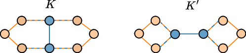
We know that the multisets of colors of 0-simplices (vertices) from and are identical at any iteration of the WL algorithm. This stems from the fact that these graphs are known to be indistiguashable by 1-WL and that the only valid neighborhood structure for vertices is the classic one (adjacent vertices) — upper-adjacency neighborhood. In other words, for each vertex in with computation tree , there is a corresponding vertex such that is isomorphic to for any depth. We also note that, in SWL, the color-refinement procedure for a vertex from upper-adjacency includes the color of the edge that is incident to. However, in our example, the color of each edge is fully defined by the history of colors of its incident vertices. Thus, we can disregard the colors of -simplices.
Similarly, if is an edge, its only neighbors are and (boundary adjacency). If we consider edges of the same colors in and , their neighbors have isomorphic computation trees. As a result, at every iteration of the test, the colors used to update these edges are exactly the same. Therefore, SWL cannot distinguish these complexes. As noted by Bodnar et al. [2021b], when SWL is applied to 1-simplicial complexes, i.e. graphs, it corresponds to the 1-WL test.
To prove that there exists a color-based filtration that distinguishes these graphs. We can directly leverage Theorem 2 in [Immonen et al., 2023] to show that there is a color-disconnecting set to these graphs . If we remove the blue edges from and , they end up with different numbers of connected components. This concludes the proof.
D.2 Proof of Proposition 2
Consider a geometric simplicial complex and geometric -simplex-color filtrations induced by a function . Let be a group element that acts on the -simplex positional features. Recall that geometric -simplex-color filtrations leverage a function , which is invariant to group actions. Thus, for any simplex , we have that . The diagrams of any dimension are fully determined by the filtrations, which in turn are obtained from the simplex rank function as
| (19) |
Note that group actions only affect geometric -simplex-color filtrations via the input of the function. Thus, we can write
| (20) |
Recalling that invariant features remain intact via the transformation, this would imply , which would lead to identical filtrations and, consequently, the same persistence diagrams (of any dimension) and topological embeddings. This holds for any .
Appendix E Approximation Error Bounds
Below are the bounds for the TOGL and RePHINE cases. Note that we assume a fixed simplicial complex for deriving the bound.
E.1 TOGL
E.1.1 Continuous Counterpart
The dynamics of the TOGL-GNN for a node can be described as,
| (21) |
For clarity of exposition, let , where is the aggregated message as described in Section 5. The continuous depth counterpart can be written as a graph ODE, parametrized by the following differential equation,
| (22) |
E.1.2 Error Bound
We consider N-layered TOGL GNN and assume an Euler discretization scheme for the ODE system consisting of steps to be consistent. We define , where is the step size and, represents a time at step. We utilize the Taylor expansion as,
| (23) |
We consider a simple modification of the discrete TOGL GNN network for -depth by letting the mapping explicitly depend on the depth of the network as,
| (24) |
We consider the error , where is the node embeddings after TOGL-GNN layers,
| (25) | ||||
| (26) | ||||
| (27) | ||||
| (28) |
We assume , to be -Lipschitz (, due to the composition of and ), giving us, (note that the parametrization of and is the same, and only differs in inputs.)
| (29) | ||||
| (30) |
Using the discrete Gronwall lemma [Sander et al., 2022, Demailly, 2006], we get the following relation, where ,
| (31) | ||||
| (32) |
But, , using that we get,
| (33) |
E.2 RePHINE
E.2.1 Continuous Counterpart
The dynamics of RePHINE-GNN for node can be expressed as,
| (34) | ||||
| (35) |
Let , where is the aggregate as described in Section 5 and . Moreover, collecting all node updates, the recursive update can be expressed as , where are the message updates for the all node embeddings. RePHINE parameterizes each layer filtration function and DeepSet function distinctively. The continuous depth counterpart can be written as a coupled latent graph ODE, parametrized by the following set of differential equations as,
| (36) | ||||
| (37) |
E.2.2 Error Bound
We consider N layered RePHINE GNN, and assume an Euler discretization scheme for the ODE system consisting of steps to be consistent. We define , where is the step size and, represents a time at step. We derive the error bounds both for the node features and topological embeddings as follows.
Node Embeddings
We utilize the Taylor expansion, as,
| (38) |
We consider a simple modification of the discrete RePHINE GNN network for -depth by letting the mapping explicitly depend on the depth of the network as,
| (39) |
We consider the node-embedding error, ,
| (40) | ||||
| (41) | ||||
| (42) |
Assuming to be -Lipschitz, gives us (note that the parametrization of and is the same, and only differs in inputs.)
| (43) | ||||
| (44) |
Using the discrete Gronwall lemma, we get the following relation, where ,
| (45) | ||||
| (46) |
But, , using that we get,
| (47) |
Topological Embeddings
We consider the bound on topological-embedding in this section. Let is the topological-embedding after RePHINE-GNN layers, the error bound can be computed as,
| (48) | ||||
| (49) |
Now, using the Taylor expansion to expand the second term, we can write ()
| (50) |
Putting into the original equation, we get,
| (51) | ||||
| (52) |
We simplify each term as follows,
First Term: The first term denotes the difference between the topological embeddings, and we assume that , as both functions are evaluated at the layer (step), and let it be -Lipschitz (, due to the composition of and ) at the time-step, giving us
| (53) | ||||
| (54) |
Second Term: We simplify the second term as follows, by adding and subtracting a term as,
| (55) | ||||
| (56) |
where the parts of the second term can be simplified as,
| (57) |
Similarly, the other term,
| (58) |
leading to . So, the equation will become,
| (59) | ||||
| (60) |
Collecting all the terms, it will account for,
| (61) |