Klingelbergstrasse 82, CH-4056 Basel, Switzerlandbbinstitutetext: Albert Einstein Center for Fundamental Physics, Institute for Theoretical Physics,
University of Bern, CH-3012 Bern, Switzerland
Flavor Hierarchies From SU(2) Flavor and Quark–Lepton Unification
Abstract
In our recent attempt to explain flavor hierarchies Greljo:2023bix , a gauged SU(2) flavor symmetry acting on left-handed fermions provides a ground to introduce three independent rank-one contributions to the Yukawa matrices: a renormalizable one for the third family, a mass-suppressed one for the second family, and an additional loop-suppressed factor for the first family. Here, we demonstrate how minimal quark-lepton unification à la Pati-Salam, relating down-quarks to charged leptons, can significantly improve this mechanism. We construct and thoroughly analyze a renormalizable model, performing a comprehensive one-loop matching calculation that reveals how all flavor hierarchies emerge from a single ratio of two scales. The first signatures may appear in the upcoming charged lepton flavor violation experiments.
1 Introduction
The peculiar pattern of fermion masses and their mixing under electroweak (EW) interactions stands as a riddle at the heart of the Standard Model (SM), known as the Flavor Puzzle. All the flavor of the SM stems from Yukawa couplings of the three generations of fermions with the single Higgs field. Contrary to naive expectations, there are large hierarchies between the size of the coupling parameters, although no power counting is suggested by the model. Observations indicate a consistent mass hierarchy of approximately two orders of magnitude between consecutive generations of all electrically charged fermions: up quarks, down quarks, and charged leptons. Also, the misalignment between the up- and down-quark Yukawa matrices, as captured by the Cabibbo–Kobayashi–Maskawa (CKM) matrix Cabibbo:1963yz ; Kobayashi:1973fv , is characterized by hierarchies between diagonal and off-diagonal elements spanning three orders of magnitude in total.
The assumption of an underlying Beyond the Standard Model (BSM) explanation for these hierarchies may provide a valuable hint as to the nature of new physics, and there has been no lack of effort in this direction; Refs. Froggatt:1978nt ; Weinberg:1972ws ; Barr:1990td ; Babu:1990hu ; Kaplan:1991dc ; Leurer:1992wg ; Leurer:1993gy ; Kaplan:1993ej ; Barbieri:1994cx ; Barbieri:1995uv ; Barbieri:1996ae ; Barbieri:1996ww ; Barbieri:1999pe ; Randall:1999ee ; Arkani-Hamed:1999ylh ; King:2003rf ; Grinstein:2010ve ; Feruglio:2015jfa ; Calibbi:2016hwq ; Ema:2016ops ; Panico:2016ull ; Bordone:2017bld ; Greljo:2018tuh ; Linster:2018avp ; Allanach:2018lvl ; Alonso:2018bcg ; Greljo:2019xan ; Smolkovic:2019jow ; Baur:2019kwi ; Fedele:2020fvh ; Nilles:2020nnc ; King:2020qaj ; Baker:2020vkh ; Babu:2020tnf ; Feruglio:2021dte ; Altmannshofer:2021qwx ; Davighi:2022fer ; Cornella:2023zme ; Asadi:2023ucx ; Davighi:2023evx ; Davighi:2023iks ; Barbieri:2023qpf ; Fuentes-Martin:2024fpx ; Altmannshofer:2022aml constitute a representative selection of early and recent examples. The goal of the flavor model building is to explain the many hierarchies observed in the fermion masses and mixings from a few (or no) ultraviolet (UV) hierarchies. We would judge the success of a mechanism based on how simple its UV realizations are and how well it produces the SM flavor pattern.
In physics, structures resulting from symmetries are widespread. Indeed, a compelling idea put forward very early on is that flavor hierarchies are a consequence of (accidental or gauged) flavor symmetries Froggatt:1978nt . Relatively simple breaking patterns may be obtained from a horizontal symmetry discriminating between the third and light generations Babu:1990hu ; Barbieri:1995uv . It was recently observed Greljo:2023bix ; Antusch:2023shi that imposing a single symmetry, which charges only one chirality of leptons and quarks respectively, still results in an accidental Feldmann:2008ja ; Kagan:2009bn ; Barbieri:2011ci ; Barbieri:2012uh ; Blankenburg:2012nx ; Fuentes-Martin:2019mun ; Faroughy:2020ina ; Greljo:2022cah of the SM Yukawa couplings in agreement with observations, allowing for a remarkably simple UV realization of the underlying mechanism. The key premise is to charge only the EW doublet on the quark side, which is involved in both the up and down Yukawa interactions. This minimal assignment generates the desired mass hierarchies and, at the same time, perturbative left-handed mixings entering the CKM matrix.
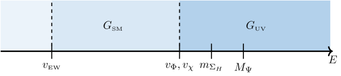
The model of Greljo:2023bix is based on an gauge symmetry under which the two light generations of left-handed quarks and leptons each form a doublet. This provides a basis to introduce three independent rank-one contributions to the Yukawa matrices, as shown in Fig. 1. To begin with, the Higgs field can directly couple (and give mass) only to the third-generation fermions at the renormalizable level. Suppressed Higgs couplings with light generations are generated through the introduction of a symmetry-breaking scalar doublet, whose vacuum expectation value (VEV) breaks . In particular, the inclusion of heavy vector-like quark and lepton fields generates at the tree level an effective dimension-5 operator between the flavor-breaking scalar, the Higgs, and light fermions; see Fig. 1 (center). When a single copy of vector-like fermions (VLFs) is present, the corresponding rank of the Yukawa matrices is only raised by one unit, generating small non-zero Yukawa couplings for the second generation only.

In the final step, the effective Yukawa couplings for the first generation are loop-generated, reusing the same vector-like fermions; see Fig. 1 (right). A clever construction that does not generate any additional unsuppressed dimension-5 operators (which might cause degeneracy between the light generation masses) is to complete the loops with new scalar leptoquark fields, such that a vector-like lepton (quark) enters that diagrams for the effective quark (lepton) Yukawa couplings. Technically, the dominant effect comes from the renormalization group mixing from a tree-level operator obtained after integrating out vector-like fermions solely. Remarkably, as long as the leptoquarks are lighter than the vector-like fermions, the hierarchy between the first two families is approximately a loop factor with a slight (logarithmic) dependence on the mass ratio.
The model proposed in Ref. Greljo:2023bix manages to explain the six mass hierarchies between consecutive generations of fermions in addition to the three hierarchies between the CKM matrix elements. All of this is in terms of two small input parameters and , the ratios of the flavor symmetry-breaking scale to the two vector-like fermion masses. The similarity of the down quark and charged lepton mass hierarchies imply , which, in this model, requires the two independent vector-like fermion masses to coincide. The model involves a single new gauge symmetry, SM, and six new matter fields. At first, this might seem unnecessarily convoluted compared to some mechanisms to explain the flavor puzzle, but when judging realizations in UV complete models, it compares very favorably. In fact, it admits further simplification and unification, as we have detailed in this paper.
The field content of the model Greljo:2023bix is very suggestive of a minimal quark–lepton unification in the manner of Pati–Salam Pati:1974yy embedding color, lepton number and baryon number into an gauge group, but without introducing Smirnov:1995jq ; FileviezPerez:2013zmv . The embedding of the gauge groups collects both vector-like fermions into a single vector-like fourplet, thereby explaining the coincidence of scales between the two, predicting . Additionally, the four scalar fields introduced in the original model are embedded into just two scalar multiplets. Quark–lepton unification thus provides a simple extension to the model, reducing the BSM matter content to four new fields and further unifying the SM chiral fermions.
The goal of the present paper is to embed the model of Ref. Greljo:2023bix into the gauge group, unifying quarks and leptons. We will demonstrate how the SM flavor structure emerges from a single hierarchy in the UV. A full-fledged renormalizable model is defined in Section 2, while the matching calculation of the effective SM Yukawa couplings is presented in Section 3. In Section 4, we show how the SM masses are recovered from a probability distribution by varying order-one parameters. Finally, in Section 5, we discuss and muon conversion on heavy nuclei as the main phenomenological constraints on the model, pointing to a symmetry-breaking scale above a few PeV. Future sensitivity in upgraded muon conversion experiments provides an opportunity for discovery if the flavor-breaking scale is low enough. Conclusions are left for Section 6 while the details of the scalar potential are relegated to the Appendix.
2 The model: Quark–lepton unification with gauged flavor
As a starting point for our model, we embed and into an gauge group in the manner of Pati and Salam Pati:1974yy , identifying leptons with a “fourth color”. The SM hypercharge emerges from the product of with a new Abelian group acting on the right-handed SM fermions. At low scales, we expect to find the SM symmetry embedded as . This construction corresponds to the minimal quark–lepton unification Smirnov:1995jq ; FileviezPerez:2013zmv ; FileviezPerez:2023rxn and can manifest at energies as low as the PeV-scale. The gauge group is further augmented with the of the SM in addition to the that acts on the two light generations of the left-handed SM fermions Babu:1990hu ; Greljo:2023bix . The latter group is the origin of the flavor structure of the model and is responsible for producing the SM mass hierarchies. Thus, the UV gauge group is given by
| (1) |
The full matter content of our theory is shown in Table 1. The SM fermions fit into the four irreducible representations under : for the two light generation left-handed fermions which form an doublet; for the third generation left-handed fermions; three copies of make up all generations for the down-type quarks and charged leptons; and three copies of , which contain the three right-handed up-type quarks. To complete , one must also include three right-handed neutrinos in the SM field content. We postpone the discussion of neutrino masses and mixings to Section 4.3. In order to generate the correct flavor structure, we additionally include a single vector-like fermion , which transforms as the third-generation left-handed fermions.
| [] Field | ||||
The flavor hierarchies of Greljo:2023bix were produced through the use of five scalar fields. These fields can be embedded into just two irreducible representations of : and . Two additional scalars are required, so our model comprises four scalar fields: , which is used to break to ; , which is used to break the EW symmetry and provide fermion masses; , which contains both the leptoquarks that run in the loops as well as an additional Higgs that can split the masses between the quark and lepton sectors; and, lastly, , which contains additional necessary leptoquarks and is used to break the flavor symmetry . The scalar field contains an SM singlet component , the VEV of which will break the flavor symmetry. At first glance, it seems like the inclusion of is not a minimal configuration since it is sufficient for and a doublet to develop VEVs to break into the SM gauge group. However, to provide masses to the first generation as shown in Greljo:2023bix , we need the leptoquark , which is a triplet under the color symmetry and a doublet under the flavor symmetry. contains both and and is, therefore, the smallest representation that simultaneously ensures the breaking of the flavor symmetry and the masses for the first family. For the decomposition of the fields under , see Table 2.
As per usual in non-supersymmetric BSM models with new scalar states, the scalar potential in our model is rather complicated and contains in excess of 60 free parameters; we refer the reader to Appendix A for the full potential. Of these there are only four parameters with the mass dimension, which control the scales on the model (see Fig. 2). The rest are marginal couplings and are assumed to be of , apart from complying with the vacuum stability and perturbative unitarity bounds. With the full potential in hand, we solved the tadpole equations and verified that our VEV configuration does indeed minimize the potential. Scanning through the parameter space, we easily find suitable points that produce condensates for , , and one of the Higgses while still ensuring all other scalar fields obtain positive masses.
| [] UV Field | Component | ||||
|---|---|---|---|---|---|
It is rather simple to organize the symmetry-breaking pattern: A non-zero VEV of is responsible for the breaking to . With an rotation, the VEV can always be arranged such that
| (2) |
In the broken phase, the adjoint scalar fields then decompose as in Table 2. In matrix form
| (3) |
where for any doublet we use the notation , and is the diagonal generator of in the fundamental representation,
| (4) |
In Greljo:2023bix , the masses for the first family are generated through the use of three leptoquarks: . These leptoquarks are embedded into the adjoint fields , with the only difference being that the latter contains two leptoquarks with the quantum numbers of . To break the flavor symmetry in the same way, develops a VEV according to
| (5) |
The placement of the VEV picks out light flavors.
The flavor hierarchies are controlled by , where is the VLF mass. There is freedom in choosing . However, simple naturalness considerations of the scalar potential suggest since the portal operators generically transmit VEVs into dimensionful couplings among the remaining scalars.444Scalar leptoquarks entering the loop diagrams for the first family masses (Fig. 1 right) must have a mass no larger than . Otherwise, the hierarchy between the first two families becomes excessively large. For scalar quartics, this condition implies . Thus, without tuning, the breaking can not be decoupled from the flavor breaking when assuming all dimensionless couplings are . Thus, for simplicity, we will assume that and develop VEVs at the same scale, as expected in the absence of tuning. As we will see in Section 5, current experimental data indicates that the symmetry-breaking should occur at the PeV scale or higher.
Indeed, it is an experimental necessity that the EW symmetry breaking occurs at a much lower scale than the breaking of to (see Section 5). Admittedly, a tuning of the scalar potential is required in order to get such a separation of scales of more than three orders of magnitude. This is an irreducible problem known to all BSM models with fundamental scalars in the absence of a protection mechanism such as supersymmetry, and we will not resolve this issue here. After the gauge symmetry breaks to , the two Higgs fields get an effective mass matrix
| (6) |
mixing the two components. The diagonal components receive contributions from various quartic interactions with and insertions, which, for our purposes, are simply absorbed into the mass terms. A realistic limit with an SM-like Higgs boson is obtained when . This ensures a small but non-zero mixing between the two states, where we consider a single tuning of to ensure that the state consisting mostly of gets a small, negative mass, thereby developing an EW symmetry-breaking VEV. In this scenario, the ratio between VEVs of and is given by
| (7) |
where . A modest order of magnitude difference in the scales and , easily gives without any additional tuning. A small is particularly interesting for phenomenology, as will be discussed in Section 4, suggesting . A rough sketch of a realistic benchmark for the various scales is shown in Fig. 2.
3 Matching to the SM Yukawas
The fermion masses are generated through a combination of renormalizable and dimension-5 effective operators produced at both tree and one-loop levels, starting from the UV Lagrangian and integrating out heavy fields. We will examine these contributions individually and establish their role in determining the rank of the mass matrices.
3.1 Rank 1
The symmetries of the model only allow the third generation to acquire masses at the renormalizable level. The relevant Yukawa interactions are
| (8) |
We denote the couplings to the singlet Higgs field with lowercase letters and the couplings to the adjoint Higgs field with uppercase letters. When the EW symmetry is broken by the Higgs fields developing VEVs, the resulting SM Yukawa matrices () will depend on a fixed linear combination of the vectors and . Importantly, these will contribute only to the third rows, resulting in the Yukawa matrices having rank 1.
3.2 Rank 2
To raise the rank of the Yukawa matrices and provide the second generation with masses, we make use of the renormalizable interactions between the VLF and the scalar fields. After integrating out , we will be left with dimension-5 operators that generate masses for the second generation. The relevant part of the Lagrangian for the matching calculation is
| (9) |
By redefining fields, we have chosen a basis with no mass mixing between and . In addition, note that and share quantum numbers. Thus, the kinetic term for exhibits an accidental symmetry. We exploit this symmetry by choosing a basis where , ensuring that the first generation of fermions remains massless at the tree level. Integrating out at the tree level, we are left with the dimension-5 operators
| (10) |
3.3 Rank 3
Already at the one-loop level, the rank of the mass matrices is increased to 3. As a result, the first family becomes massive, and the loop factor nicely explains the hierarchy between the two light families. Even though the same couplings from Eq. (9) are involved in the loop diagrams (see Fig. 1 right), the leptoquark contributions, together with the independent scalar quartics, provide enough freedom to raise the rank and correctly fit the first-family parameters. We use Matchete Fuentes-Martin:2022jrf to compute the effective dimension-5 Yukawa operators at the one loop. Due to their length and complexity, we only list one of the representative terms which increases the rank:
| (11) |
When the scalar fields develop VEVs, the leading expressions for the resulting mass matrices are rather simple and will be presented in full below.
3.4 The mass matrices
The fermion masses are generated after the Higgs doublets develop VEVs according to
| (12) |
will contribute equally to the quark and lepton sectors since it is a singlet under , while will split the down-quark and charged-lepton masses since it is embedded in the adjoint field .
Utilizing the remaining freedom to rotate the right-handed fields, , we choose a basis where the tree-level quark Yukawa matrices are upper-triangular,555The conditions are and where .
| (13) |
Including the one-loop results only for the first generation, where it makes the difference, we finally get
| (14) |
Here
| (15) |
are the suppression factors associated with the tree-level and one-loop operators, respectively, and
| (16) |
Note that the quark mass matrices are upper-triangular with the hierarchical rows, which ensures small left-handed rotation matrices in agreement with the CKM matrix.
In our chosen basis, the charged lepton mass matrix is not upper-triangular due to its dependence on the same Yukawa couplings as the down-type quark mass matrix, i.e., is already used up to set the latter into a desired form. Therefore,
| (17) |
where
| (18) |
4 Producing the flavor hierarchies
Starting from the mass matrices in Eqs. (14) and (17), in Section 4.1, we will derive quark and charged-lepton masses and the CKM elements in terms of the UV parameters. Subsequently, in Section 4.2, we will conduct a detailed numerical scan of the UV parameter space to predict the SM flavor hierarchies. Finally, we will discuss the neutrino sector in Section 4.3.
4.1 Perturbative diagonalization
Since the quark mass matrices are upper-triangular with hierarchical rows, we perturbatively diagonalize them to obtain the quark masses and the CKM matrix. The perturbative diagonalization is performed as described in the Appendix of Ref. Greljo:2023bix , and we report only the leading terms in expansion. The singular value decomposition gives us the rotation matrices through
| (19) |
where is diagonal. The upper-triangular structure of the quark mass matrices ensures that the off-diagonal elements of are negligible, while the hierarchy between the rows ensures that the off-diagonal elements of are small and hierarchical, satisfying
| (20) |
The CKM matrix is then determined by . From the diagonal , we get the quark masses
| (21) | ||||||
| (22) | ||||||
| (23) |
While using the full expression in the numerical scan, we omit writing it here due to its complexity and only note that it satisfies at the leading order.
The left-handed rotations in the lepton sector are also small and hierarchical due to the hierarchies between the rows in Eq. 17. By contrast, the right-handed rotations are can be sizeable depending on the region of parameter space. Consider now the limit , in which becomes upper-triangular, causing the right-handed rotations to be negligible. In this limit it follows from Eqs. 14 and 17 that the third rows of and become identical while the first two rows differ only by a multiplicative factor. In this limit, . Empirically, the bottom-tau unification is remarkably successful at high energies, which is the primary motivation for considering this limit. However, obtaining the correct size necessitates restricting . As we will demonstrate in the numerical scan below, this is the only dimensionless parameter that must be somewhat small compared to expectations. In fact, as long as , only a single parameter needs to be tuned. For , four parameters must be restricted to magnitudes of , see Eq. 17. Finally, the limit predicts a wrong mass ratio and is ruled out. In the numerical studies, we will focus on .
4.2 Numerical scan
We randomly generate one million parameter points from a flat distribution, applying the following constraints on the dimensionless couplings in the UV Lagrangian: , , and all other contributing Yukawa and scalar couplings are allowed to be complex, with their magnitudes constrained to . We take the symmetry breaking and the renormalization scales equal, , and fix the ratio between the VLF mass and the symmetry breaking scale to . Additionally, we set , but we have verified that the results remain qualitatively unchanged as long as .
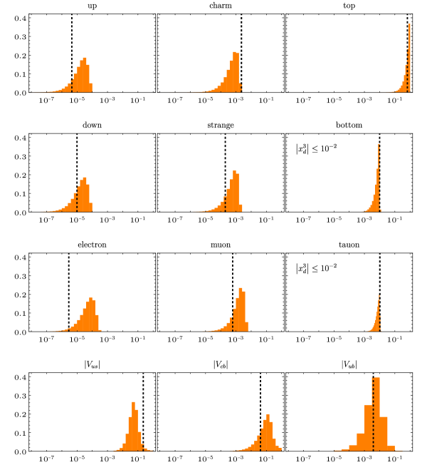
In Fig. 3, we plot the predicted histograms for the SM flavor parameters. The first three rows display the values of the Yukawa couplings, , while the fourth row shows the magnitudes of the CKM elements. The black solid lines represent the singular values of the running SM Yukawa couplings at the renormalization scale as given in Greljo:2023bix , and the CKM matrix elements, which do not run significantly, as provided by the PDG Workman:2022ynf . These distributions illustrate the overall satisfactory agreement between the predicted and observed parameters. Somewhat ad-hoc restriction of a single parameter is critical; otherwise, for , the bottom-quark and tau distributions would look like the top-quark distribution, shown in the first row, third column.
By repeating a similar exercise with other parameters, we confirmed that the structure is primarily controlled by , with only a mild dependence on other parameters. The varying broadness of the distributions between for different generations is due to the fact that the first, second, and third family Yukawas are proportional to a product of three, two, and to a single UV coupling, respectively (see Fig. 1). Remember that their magnitudes are drawn from a uniform distribution in the range.
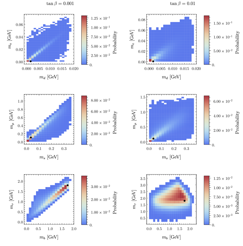
Another interesting aspect is revealed when studying the correlations between the observed parameters. To visualize the effect that has on the bottom-tau splitting, we generated one million parameter points for two different values of : and while other configurations of the scan remain unchanged. In Fig. 4, we present histograms showing the correlation between the masses of the down-type quarks and charged leptons. The black dot marks the running masses at the appropriate scale. In the limit, there is a strong correlation across all three generations, which is in remarkable agreement with observations! Increasing decreases the correlation, and this effect is most noticeable for the third generation.
4.3 Neutrino sector
Up to this point, we have focused on the flavor structure in the charged fermion sector, neglecting the neutrino masses and the Pontecorvo–Maki–Nakagawa–Sakata (PMNS) Maki:1962mu mixing matrix. Unlike the hierarchies observed in the charged sector, the neutrino flavor appears to be anarchic. Indeed, the PMNS matrix stands in stark contrast to the CKM matrix, exhibiting large mixing angles. Arguably, the only relevant hierarchy in the neutrino sector is related to the overall neutrino mass scale, which is many orders of magnitude below the electron mass. In this section, we will briefly discuss how to correctly reproduce neutrino parameters within this model.
At face value, the model predicts a Dirac mass matrix
| (24) |
for the neutrinos, where
| (25) |
This alone incorrectly implies that neutrino masses are similar in size to the up-quark masses, and the PMNS matrix is close to a unit matrix.
An elegant explanation of the smallness of neutrino masses in the context of minimal quark-lepton unification is provided by the inverse seesaw mechanism FileviezPerez:2013zmv . Our model is minimally expanded by introducing three left-handed gauge-singlet fermions (). As a result, the Lagrangian gets supplemented by the following gauge-invariant and renormalizable operators:
| (26) |
where . We define , where denotes charge conjugation. The neutral lepton mass matrix, which is , is given by
| (27) |
The global lepton number is an approximate symmetry softly broken by . For , the mass matrix for active neutrinos approximates to
| (28) |
Thus, the overall smallness of the neutrino masses is explained by the small breaking of the lepton number via . It is evident that the observed neutrino mass splittings and the PMNS mixing angles can be accurately fitted by introducing hierarchies into , given that is hierarchical. The origin of these hierarchies is beyond the present work.
5 Phenomenology
The symmetry-breaking scale of our model is constrained by rare processes mediated by the massive vector bosons resulting from this breaking. In Pati–Salam-type models, the vector leptoquarks are known to give contributions to the lepton flavor–violating decay , which is forbidden in the SM. This typically constrains the breaking scale to be of the order of a few PeV Valencia:1994cj ; Smirnov:2007hv , and we will see that this general picture is reproduced here. The vector bosons are also known to give unsuppressed contributions to these SM-forbidden decays through a mechanism known as flavor transfer Darme:2023nsy ; Greljo:2023bix , but the resulting bound on is weaker as we will show below. Typical rotations into the fermion mass basis will also result in contributions to muon conversion on heavy nuclei, a stringently constrained process with great potential for improvements in planned experiments.
Integrating out the vector leptoquark and the flavored at tree level results in effective operators
| (29) |
at the high scale, where is the generator of rotations in the fundamental representation. We assume here that the right-handed neutrinos are too heavy to play a role in low-energy flavor physics and have ignored their contributions accordingly. Next, we transition to the low-energy effective Lagrangian (LEFT) below the scale of EW symmetry breaking to get to the mass basis fermions at the scale relevant to the lepton flavor–violating processes discussed above. Only the semi-leptonic operators are relevant and shown here:666We have omitted a contribution to the left-handed vector operator proportional to , as lepton flavor–violating contributions from this term are severely suppressed on account of a GIM-like mechanism.
| (30) | ||||
where . The numerical factor of on the second line is a combination of a factor of from Fierzing the four-fermion operator and a factor of from running the operator down from to (as determined with DsixTools Celis:2017hod ; Fuentes-Martin:2020zaz ). By contrast, the vector current operators barely run at all (shifting only the operators by a few percent), and we disregard that effect.
5.1 Lepton flavor–violating kaon decay
The non-observation of the decay poses a strong constraint on the scale of symmetry breaking. The current experimental bound on the branching rate is @ 90% CL BNL:1998apv . We calculated the NP contribution to this decay rate from the LEFT Lagrangian in Section 5 using Ref. Marzocca:2021miv and obtained
| (31) | ||||
having normalized the VEVs by . The pseudo-scalar quark current interpolates better than the axial vector, resulting in a significant enhancement to the contributions stemming from mixed left–right currents due to the vector leptoquark, which are also enhanced by the RG running.777These are the contributions multiplying .
With no suppression of the NP contribution from the fermion rotation matrices, the branching ratio in Section 5.1 bounds . However, it may be possible to evade this constraint. In a simple approximation, where and are taken to be two-dimensional rotation matrices (dominated by the 1–2 rotation angle), the scalar contribution will vanish altogether if the rotation angles are orthogonal. While the left-handed rotations are perturbative and, therefore, close to the identity matrix, the right-handed rotation might be close to maximal, leading to a vanishing scalar contribution. In this case, the bound will come from the vector currents constraining . That being said, we consider the realizations with the symmetry-breaking scale of at least a PeV to be the more realistic scenario.
5.2 Muon conversion on heavy nuclei
Muon conversion on heavy nuclei is closely correlated to the lepton flavor–violating kaon decay, which is also caused by the Lagrangian in Section 5, but without any quark flavor violation. The SINDRUM-II experiment set the best present bound on this process, obtaining the limit for the conversion rate in muonic gold SINDRUMII:2006dvw . Scalar and vector four-fermion operators contribute to this process at roughly the same rate, and, using Ref. Kitano:2002mt , we determine the contribution from the heavy vector bosons:
| (32) | ||||
The numerical enhancement of the scalar operators is due to the RG-running already present in the Wilson coefficients in Section 5.
Muon conversion violates lepton flavor by one unit while quark flavor is conserved. Thus, in the interaction basis, the process would be forbidden, as no flavor transfer Darme:2023nsy is possible. We should, however, expect a mixing of at least the left-handed down-type in order to recover the sizable Cabbibo angle. In the limit, where the is the only non-trivial mixing, the NP contribution in Eq. 32 gives the bounds and . While specific realizations of the mixing matrices may either enhance or weaken the bounds, they are a good estimate for realistic benchmarks in the absence of tuning. Interestingly, the future Mu2e Bernstein:2019fyh and COMET Moritsu:2022lem experiments projects an improvement on the experimental sensitivity to the level of .888Both Mu2e and COMET will be using aluminum as the target nuclei, changing the numerical factors in Eq. (32). Hence, the experimental sensitivity to the symmetry-breaking scales is expected to improve by an order of magnitude. This provides an exciting avenue for experimentally detecting the imprints of the model behind the flavor structure posited in this paper.
6 Conclusion
The field of flavor physics has a bright future due to a comprehensive experimental program anticipated within this decade. The interest is driven by the potential to detect indirect effects of heavy BSM physics from scales well beyond the reach of direct searches. Indirect signs of new physics might manifest in phenomena such as rare flavor-changing neutral currents, violations of charged lepton flavor, and electric dipole moments, each of which is expected to see substantial experimental advancements LHCb:2018roe ; LHCb:2021glh ; Belle-II:2018jsg ; Forti:2022mti ; Belle-II:2022cgf ; NA62KLEVER:2022nea ; MEGII:2018kmf ; Bernstein:2019fyh ; Moritsu:2022lem ; n2EDM:2021yah ; Wu:2019jxj ; Blondel:2013ia ; ACME:2018yjb ; EuropeanStrategyforParticlePhysicsPreparatoryGroup:2019qin . Furthermore, flavor physics is closely tied to some of the most significant structural challenges of the SM. The origin of flavor remains an enduring enigma: one of the most puzzling aspects is the presence of hierarchies in the masses (and mixings) of charged fermions between successive generations, despite all of them arising from the Yukawa interactions with a single Higgs field. This longstanding puzzle has attracted a renewed interest in light of recent experimental activities.
Perhaps the resolution of the flavor puzzle may lie already at the next hidden layer of nature. It is worthwhile to explore novel possibilities for low-scale flavor models, which could lead to deviations detectable in forthcoming experiments. In this paper, we construct and thoroughly investigate one particularly elegant example. Building upon our recent work Greljo:2023bix , we combine a gauged flavor symmetry with a minimal quark-lepton unification paradigm based on the gauge group. The flavor symmetry acts on left-chiral fermions, distinguishing the light-family doublet from the third-family singlet. The model, detailed in Section 2, predicts hierarchically distinct contributions to the rank of the Yukawa matrices, which then translates into the hierarchies between families.
As illustrated in Fig. 1, the third row in the Yukawa matrices results from unsuppressed dimension-4 Yukawa interactions. The second row emerges from integrating out a single heavy vector-like fermion, yielding a tree-level dimension-5 operator. The first row is populated by loop diagrams involving the same fields and generating a loop-level dimension-5 operator. The matter field content required to realize this mechanism is remarkably minimal, as shown in Table 1. This is due to the elegant unification of multiple elements from Ref. Greljo:2023bix collected in Table 2.
The entire SM flavor structure is controlled by a single parameter , a ratio of the flavor-breaking scale to the VLF mass. After performing a detailed matching calculation to the SM Yukawas in Section 3, we conduct a comprehensive numerical scan in Section 4. The key result is presented in Fig. 3, showing a histogram of predictions for SM flavor parameters, for , obtained from randomly selecting dimensionless UV couplings from a flat distribution in the range . Remarkably, reasonable order-of-magnitude predictions emerge for all measured parameters, except for the Yukawa, which requires a single UV parameter to be somewhat smaller than expected, . Even more remarkable is the predicted correlation between down-quark and charged lepton masses shown in Fig. 4. For a small ratio of Higgs VEVs, , this correlation is very precise and shows an extraordinary agreement with the measured values. This exemplifies how quark-lepton unification, a well-motivated concept on its own, aids in explaining the flavor puzzle.
As demonstrated in Section 5, the leading signatures of the model are lepton flavor–violating kaon decays and muon conversion on heavy nuclei, where the experimental prospects are excellent. In fact, current limits already require the scale of the model to be at least of the order of PeV, which introduces another hierarchy problem related to the smallness of the electroweak scale. Additionally, generating small neutrino masses can be straightforwardly achieved using the inverse see-saw mechanism, as described in Section 4.3. However, predicting large PMNS mixing angles requires additional structure. These issues are not addressed in this work and are left for future research.
Acknowledgments
This work has received funding from the Swiss National Science Foundation (SNF) through the Eccellenza Professorial Fellowship “Flavor Physics at the High Energy Frontier,” project number 186866, and the Ambizione grant “Matching and Running: Improved Precision in the Hunt for New Physics,” project number 209042.
Appendix A Scalar potential
To find the full scalar potential and ensure that no superfluous terms were included or any possible terms omitted, we made use of the Mathematica package Sym2Int Fonseca:2017lem . We have used Roman letters for indices: , and Greek letters for indices: , and surpressed all other indices. The full scalar potential is given below:
| (33) |
References
- (1) A. Greljo and A.E. Thomsen, Rising through the ranks: flavor hierarchies from a gauged SU(2) symmetry, Eur. Phys. J. C 84 (2024) 213 [2309.11547].
- (2) N. Cabibbo, Unitary Symmetry and Leptonic Decays, Phys. Rev. Lett. 10 (1963) 531.
- (3) M. Kobayashi and T. Maskawa, CP Violation in the Renormalizable Theory of Weak Interaction, Prog. Theor. Phys. 49 (1973) 652.
- (4) C.D. Froggatt and H.B. Nielsen, Hierarchy of Quark Masses, Cabibbo Angles and CP Violation, Nucl. Phys. B 147 (1979) 277.
- (5) S. Weinberg, Electromagnetic and weak masses, Phys. Rev. Lett. 29 (1972) 388.
- (6) S.M. Barr, A Predictive hierarchical mode of quark and lepton masses, Phys. Rev. D 42 (1990) 3150.
- (7) K.S. Babu and R.N. Mohapatra, Radiative fermion masses and large neutrino magnetic moment: A Unified picture, Phys. Rev. D 43 (1991) 2278.
- (8) D.B. Kaplan, Flavor at SSC energies: A New mechanism for dynamically generated fermion masses, Nucl. Phys. B 365 (1991) 259.
- (9) M. Leurer, Y. Nir and N. Seiberg, Mass matrix models, Nucl. Phys. B 398 (1993) 319 [hep-ph/9212278].
- (10) M. Leurer, Y. Nir and N. Seiberg, Mass matrix models: The Sequel, Nucl. Phys. B 420 (1994) 468 [hep-ph/9310320].
- (11) D.B. Kaplan and M. Schmaltz, Flavor unification and discrete nonAbelian symmetries, Phys. Rev. D 49 (1994) 3741 [hep-ph/9311281].
- (12) R. Barbieri, G.R. Dvali and A. Strumia, Fermion masses and mixings in a flavor symmetric GUT, Nucl. Phys. B 435 (1995) 102 [hep-ph/9407239].
- (13) R. Barbieri, G.R. Dvali and L.J. Hall, Predictions from a U(2) flavor symmetry in supersymmetric theories, Phys. Lett. B 377 (1996) 76 [hep-ph/9512388].
- (14) R. Barbieri and L.J. Hall, A Grand unified supersymmetric theory of flavor, Nuovo Cim. A 110 (1997) 1 [hep-ph/9605224].
- (15) R. Barbieri, L.J. Hall, S. Raby and A. Romanino, Unified theories with U(2) flavor symmetry, Nucl. Phys. B 493 (1997) 3 [hep-ph/9610449].
- (16) R. Barbieri, P. Creminelli and A. Romanino, Neutrino mixings from a U(2) flavor symmetry, Nucl. Phys. B 559 (1999) 17 [hep-ph/9903460].
- (17) L. Randall and R. Sundrum, A Large mass hierarchy from a small extra dimension, Phys. Rev. Lett. 83 (1999) 3370 [hep-ph/9905221].
- (18) N. Arkani-Hamed and M. Schmaltz, Hierarchies without symmetries from extra dimensions, Phys. Rev. D 61 (2000) 033005 [hep-ph/9903417].
- (19) S.F. King and G.G. Ross, Fermion masses and mixing angles from SU (3) family symmetry and unification, Phys. Lett. B 574 (2003) 239 [hep-ph/0307190].
- (20) B. Grinstein, M. Redi and G. Villadoro, Low Scale Flavor Gauge Symmetries, JHEP 11 (2010) 067 [1009.2049].
- (21) F. Feruglio, Pieces of the Flavour Puzzle, Eur. Phys. J. C 75 (2015) 373 [1503.04071].
- (22) L. Calibbi, F. Goertz, D. Redigolo, R. Ziegler and J. Zupan, Minimal axion model from flavor, Phys. Rev. D 95 (2017) 095009 [1612.08040].
- (23) Y. Ema, K. Hamaguchi, T. Moroi and K. Nakayama, Flaxion: a minimal extension to solve puzzles in the standard model, JHEP 01 (2017) 096 [1612.05492].
- (24) G. Panico and A. Pomarol, Flavor hierarchies from dynamical scales, JHEP 07 (2016) 097 [1603.06609].
- (25) M. Bordone, C. Cornella, J. Fuentes-Martin and G. Isidori, A three-site gauge model for flavor hierarchies and flavor anomalies, Phys. Lett. B 779 (2018) 317 [1712.01368].
- (26) A. Greljo and B.A. Stefanek, Third family quark–lepton unification at the TeV scale, Phys. Lett. B 782 (2018) 131 [1802.04274].
- (27) M. Linster and R. Ziegler, A Realistic Model of Flavor, JHEP 08 (2018) 058 [1805.07341].
- (28) B.C. Allanach and J. Davighi, Third family hypercharge model for and aspects of the fermion mass problem, JHEP 12 (2018) 075 [1809.01158].
- (29) R. Alonso, A. Carmona, B.M. Dillon, J.F. Kamenik, J. Martin Camalich and J. Zupan, A clockwork solution to the flavor puzzle, JHEP 10 (2018) 099 [1807.09792].
- (30) A. Greljo, T. Opferkuch and B.A. Stefanek, Gravitational Imprints of Flavor Hierarchies, Phys. Rev. Lett. 124 (2020) 171802 [1910.02014].
- (31) A. Smolkovič, M. Tammaro and J. Zupan, Anomaly free Froggatt-Nielsen models of flavor, JHEP 10 (2019) 188 [1907.10063].
- (32) A. Baur, H.P. Nilles, A. Trautner and P.K.S. Vaudrevange, Unification of Flavor, CP, and Modular Symmetries, Phys. Lett. B 795 (2019) 7 [1901.03251].
- (33) M. Fedele, A. Mastroddi and M. Valli, Minimal Froggatt-Nielsen textures, JHEP 03 (2021) 135 [2009.05587].
- (34) H.P. Nilles, S. Ramos-Sánchez and P.K.S. Vaudrevange, Eclectic Flavor Groups, JHEP 02 (2020) 045 [2001.01736].
- (35) S.J.D. King and S.F. King, Fermion mass hierarchies from modular symmetry, JHEP 09 (2020) 043 [2002.00969].
- (36) M.J. Baker, P. Cox and R.R. Volkas, Has the Origin of the Third-Family Fermion Masses been Determined?, JHEP 04 (2021) 151 [2012.10458].
- (37) K.S. Babu and S. Saad, Flavor Hierarchies from Clockwork in SO(10) GUT, Phys. Rev. D 103 (2021) 015009 [2007.16085].
- (38) F. Feruglio, V. Gherardi, A. Romanino and A. Titov, Modular invariant dynamics and fermion mass hierarchies around , JHEP 05 (2021) 242 [2101.08718].
- (39) W. Altmannshofer and S.A. Gadam, Supersymmetric flavor clockwork model, Phys. Rev. D 104 (2021) 035030 [2106.09869].
- (40) J. Davighi and J. Tooby-Smith, Electroweak flavour unification, JHEP 09 (2022) 193 [2201.07245].
- (41) C. Cornella, D. Curtin, E.T. Neil and J.O. Thompson, Mapping and Probing Froggatt-Nielsen Solutions to the Quark Flavor Puzzle, 2306.08026.
- (42) P. Asadi, A. Bhattacharya, K. Fraser, S. Homiller and A. Parikh, Wrinkles in the Froggatt-Nielsen mechanism and flavorful new physics, JHEP 10 (2023) 069 [2308.01340].
- (43) J. Davighi and B.A. Stefanek, Deconstructed hypercharge: a natural model of flavour, JHEP 11 (2023) 100 [2305.16280].
- (44) J. Davighi and G. Isidori, Non-universal gauge interactions addressing the inescapable link between Higgs and flavour, JHEP 07 (2023) 147 [2303.01520].
- (45) R. Barbieri and G. Isidori, Minimal flavour deconstruction, JHEP 05 (2024) 033 [2312.14004].
- (46) J. Fuentes-Martín and J.M. Lizana, Deconstructing flavor anomalously, 2402.09507.
- (47) W. Altmannshofer and J. Zupan, Snowmass White Paper: Flavor Model Building, in Snowmass 2021, 3, 2022 [2203.07726].
- (48) S. Antusch, A. Greljo, B.A. Stefanek and A.E. Thomsen, U(2) Is Right for Leptons and Left for Quarks, Phys. Rev. Lett. 132 (2024) 151802 [2311.09288].
- (49) T. Feldmann and T. Mannel, Large Top Mass and Non-Linear Representation of Flavour Symmetry, Phys. Rev. Lett. 100 (2008) 171601 [0801.1802].
- (50) A.L. Kagan, G. Perez, T. Volansky and J. Zupan, General Minimal Flavor Violation, Phys. Rev. D 80 (2009) 076002 [0903.1794].
- (51) R. Barbieri, G. Isidori, J. Jones-Perez, P. Lodone and D.M. Straub, and Minimal Flavour Violation in Supersymmetry, Eur. Phys. J. C 71 (2011) 1725 [1105.2296].
- (52) R. Barbieri, D. Buttazzo, F. Sala and D.M. Straub, Flavour physics from an approximate symmetry, JHEP 07 (2012) 181 [1203.4218].
- (53) G. Blankenburg, G. Isidori and J. Jones-Perez, Neutrino Masses and LFV from Minimal Breaking of and flavor Symmetries, Eur. Phys. J. C 72 (2012) 2126 [1204.0688].
- (54) J. Fuentes-Martín, G. Isidori, J. Pagès and K. Yamamoto, With or without U(2)? Probing non-standard flavor and helicity structures in semileptonic B decays, Phys. Lett. B 800 (2020) 135080 [1909.02519].
- (55) D.A. Faroughy, G. Isidori, F. Wilsch and K. Yamamoto, Flavour symmetries in the SMEFT, JHEP 08 (2020) 166 [2005.05366].
- (56) A. Greljo, A. Palavrić and A.E. Thomsen, Adding Flavor to the SMEFT, JHEP 10 (2022) 010 [2203.09561].
- (57) J.C. Pati and A. Salam, Lepton Number as the Fourth Color, Phys. Rev. D 10 (1974) 275.
- (58) A.D. Smirnov, The Minimal quark - lepton symmetry model and the limit on Z-prime mass, Phys. Lett. B 346 (1995) 297 [hep-ph/9503239].
- (59) P. Fileviez Perez and M.B. Wise, Low Scale Quark-Lepton Unification, Phys. Rev. D 88 (2013) 057703 [1307.6213].
- (60) P. Fileviez Pérez, C. Murgui, S. Patrone, A. Testa and M.B. Wise, Finite naturalness and quark-lepton unification, Phys. Rev. D 109 (2024) 015011 [2308.07367].
- (61) J. Fuentes-Martín, M. König, J. Pagès, A.E. Thomsen and F. Wilsch, A proof of concept for matchete: an automated tool for matching effective theories, Eur. Phys. J. C 83 (2023) 662 [2212.04510].
- (62) Particle Data Group collaboration, Review of Particle Physics, PTEP 2022 (2022) 083C01.
- (63) Z. Maki, M. Nakagawa and S. Sakata, Remarks on the unified model of elementary particles, Prog. Theor. Phys. 28 (1962) 870.
- (64) G. Valencia and S. Willenbrock, Quark - lepton unification and rare meson decays, Phys. Rev. D 50 (1994) 6843 [hep-ph/9409201].
- (65) A.D. Smirnov, Mass limits for scalar and gauge leptoquarks from K(L)0 — e-+ mu+-, B0 — e-+ tau+- decays, Mod. Phys. Lett. A 22 (2007) 2353 [0705.0308].
- (66) L. Darmé, A. Deandrea and F. Mahmoudi, Gauge SU(2)f flavour transfers, JHEP 05 (2024) 313 [2307.09595].
- (67) A. Celis, J. Fuentes-Martin, A. Vicente and J. Virto, DsixTools: The Standard Model Effective Field Theory Toolkit, Eur. Phys. J. C 77 (2017) 405 [1704.04504].
- (68) J. Fuentes-Martin, P. Ruiz-Femenia, A. Vicente and J. Virto, DsixTools 2.0: The Effective Field Theory Toolkit, Eur. Phys. J. C 81 (2021) 167 [2010.16341].
- (69) BNL collaboration, New limit on muon and electron lepton number violation from K0(L) — mu+- e-+ decay, Phys. Rev. Lett. 81 (1998) 5734 [hep-ex/9811038].
- (70) D. Marzocca, S. Trifinopoulos and E. Venturini, From B-meson anomalies to Kaon physics with scalar leptoquarks, Eur. Phys. J. C 82 (2022) 320 [2106.15630].
- (71) SINDRUM II collaboration, A Search for muon to electron conversion in muonic gold, Eur. Phys. J. C 47 (2006) 337.
- (72) R. Kitano, M. Koike and Y. Okada, Detailed calculation of lepton flavor violating muon electron conversion rate for various nuclei, Phys. Rev. D 66 (2002) 096002 [hep-ph/0203110].
- (73) Mu2e collaboration, The Mu2e Experiment, Front. in Phys. 7 (2019) 1 [1901.11099].
- (74) COMET collaboration, Search for Muon-to-Electron Conversion with the COMET Experiment †, Universe 8 (2022) 196 [2203.06365].
- (75) LHCb collaboration, Physics case for an LHCb Upgrade II - Opportunities in flavour physics, and beyond, in the HL-LHC era, 1808.08865.
- (76) LHCb collaboration, Framework TDR for the LHCb Upgrade II: Opportunities in flavour physics, and beyond, in the HL-LHC era, .
- (77) Belle-II collaboration, The Belle II Physics Book, PTEP 2019 (2019) 123C01 [1808.10567].
- (78) Belle-II collaboration, Snowmass Whitepaper: The Belle II Detector Upgrade Program, in Snowmass 2021, 3, 2022 [2203.11349].
- (79) Belle-II collaboration, Snowmass White Paper: Belle II physics reach and plans for the next decade and beyond, 2207.06307.
- (80) NA62/KLEVER, US Kaon Interest Group, KOTO, LHCb collaboration, Searches for new physics with high-intensity kaon beams, in Snowmass 2021, 4, 2022 [2204.13394].
- (81) MEG II collaboration, The design of the MEG II experiment, Eur. Phys. J. C 78 (2018) 380 [1801.04688].
- (82) n2EDM collaboration, The design of the n2EDM experiment: nEDM Collaboration, Eur. Phys. J. C 81 (2021) 512 [2101.08730].
- (83) X. Wu, Z. Han, J. Chow, D.G. Ang, C. Meisenhelder, C.D. Panda et al., The metastable Q state of ThO: a new resource for the ACME electron EDM search, New J. Phys. 22 (2020) 023013 [1911.03015].
- (84) A. Blondel et al., Research Proposal for an Experiment to Search for the Decay , 1301.6113.
- (85) ACME collaboration, Improved limit on the electric dipole moment of the electron, Nature 562 (2018) 355.
- (86) R.K. Ellis et al., Physics Briefing Book: Input for the European Strategy for Particle Physics Update 2020, 1910.11775.
- (87) R.M. Fonseca, The Sym2Int program: going from symmetries to interactions, J. Phys. Conf. Ser. 873 (2017) 012045 [1703.05221].