Unconventional Scalings of Quantum Entropies in Long-Range Heisenberg Chains

Abstract

In this work, building on state-of-the-art quantum Monte Carlo simulations, we perform systematic finite-size scaling of both entanglement and participation entropies for long-range Heisenberg chain with unfrustrated power-law decaying interactions. We find distinctive scaling behaviors for both quantum entropies in the various regimes explored by tuning the decay exponent $\alpha$, thus capturing non-trivial features through logarithmic terms, beyond the case of linear Nambu-Goldstone modes. Our systematic analysis reveals that the quantum entanglement information, hidden in the scaling of the two studied entropies, can be obtained to the same level of order parameters and other usual finite-size observables of quantum many-body lattice models. The analysis and results obtained here can readily apply to more quantum criticalities in 1D and 2D systems.

Introduction.— Long-range interactions in quantum systems can give rise to unconventional quantum phases and transitions [1, 2, 3, 4, 5, 6, 7, 8, 9, 10, 11, 12, 13, 14, 15, 16, 17]. Particularly interesting is the case of low spatial dimensions $d=1,2$, where unusual behaviors can occur beyond the realm of Hohenberg-Mermin-Wagner theorem [18, 19, 20, 21, 22], such as long-range order that breaks the continuous symmetry in the ground state for $d=1$ [2], the modification of the excitation spectra [23, 13, 12, 16, 24], the breaking of the Lieb-Robinson bound of propagation of information [25, 26, 27, 28] and even the violation of area-law scaling of entanglement entropy (EE) [29, 30, 9].

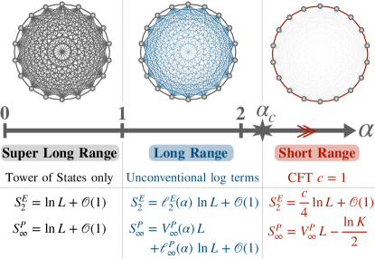
Figure 1: Schematic picture showing the succession of the three different regimes as function of the exponent $\alpha$ of the long-range couplings in Eq. (1). Left: for $\alpha\in[0,1]$, the system is over-extensive and falls in the fully connected Lieb-Mattis case [31]. Right: for $\alpha>\alpha_{c}\approx 2.23$, long-range couplings are irrelevant [2] (signaled by the red arrows) and the quasi-long-range-ordered Luttinger liquid physics is recovered with the CFT results for both EE and PE. Middle: for $1<\alpha<\alpha_{c}$, the ground-state has a true SU(2) symmetry broken long-range order, and displays finite unconventional logarithmic terms for both EE and PE. $\alpha_{c}$ is the unconventional QCP also with logarithmic corrections in the two entropies. See text for more details on the various scaling forms.

However, these exotic features in long-range systems have been discussed on a case-by-case basis, and there is a lack of systematic study of the quantum critical behavior and the scaling of the entanglement content as the interaction continuously changes from long-range to short-range. In such a case, one would like to draw a comprehensive picture which combines critical behavior with the scalings of both EE [32, 33] and the participation entropy (PE) [34, 35, 36].

Introduced in Refs. [23, 2], the unfrustrated long-range antiferromagnetic (AF) Heisenberg $S=1/2$ chain model

$${\cal{H}}_{\rm LR}(\alpha)=\sum_{i<j}J_{ij}\mathbf{S}_{i}\cdot\mathbf{S}_{j},\quad J_{ij}=\frac{(-1)^{j-i+1}}{|i-j|^{\alpha}},$$ (1)

provides an ideal test-bed to explore a very rich variety of non-trivial phenomena [2, 3, 4, 37]. Upon tuning the decay exponent $\alpha$, there is an unconventional quantum critical point (QCP) at $\alpha_{c}\sim 2.2-2.25$ [2, 3, 4] between a short-range (SR) regime described by conformal field theory (CFT) for $\alpha>\alpha_{c}$, and a long-range (LR) ordered phase for $1<\alpha<\alpha_{c}$ where the continuous SU(2) symmetry spontaneously breaks, even if we are in $d=1$. It is also worth mentioning the "over-extensive" case $\alpha\leq 1$ [38] (super-long-range), where quantum corrections to the classical AF order parameter vanish at large sizes [23], putting this regime in the same class as the fully connected Lieb-Mattis model [31], as will be discussed below.

In this work, building on both entanglement and participation entropies obtained from large-scale quantum Monte Carlo simulations [39, 40, 41], we explore how the critical properties, the entanglement content and the complexity of the many-body ground-state evolves upon changing the exponent $\alpha$ of the LR Heisenberg interaction in Eq. (1). As summarized in Fig. 1 three situations emerge, with characteristically different scalings for the two quantum entropies. While both short-range (SR) and super-long-range (super-LR) regimes can be well understood from current theoretical frameworks, the broad intermediate long-range (LR) ordered phase is much more intriguing. Indeed, in this long-range regime, and at the unconventional critical point $\alpha_{c}$, where Lorentz invariance is broken (i.e. the dynamical critical exponent $z<1$ [2, 4]), non-trivial logarithmic scalings are found for both quantum entropies EE and PE.

The rest of this Letter is organized as follows. We first revisit the critical point with standard finite-size scaling of the Binder cumulant, which allows us to locate the critical point with higher accuracy. We then discuss our QMC results for the two quantum entropies (first the EE and then the PE) over the whole regime. We clearly confirm the scaling forms for both SR and super-LR phases, and discuss in detail the extraction of the unconventional logarithmic scalings in the intermediate LR regime. Finally, we discuss the implications of our results and possible experimental consequences.

Model and Unconventional Critical Point.— The 1D LR Heisenberg model we study is defined in Eq. (1), where $J_{ij}$ represents the staggered long-range interaction which does not introduce frustrations. In practice, in order to alleviate finite-size effects, we consider the Ewald summation which modifies the couplings strength as $\tilde{J}_{ij}=\sum_{m=-\infty}^{+\infty}\frac{(-1)^{i-j+1}}{|i-j+mL|^{\alpha}}$, as has been successfully applied in long-range spin models [42, 43, 44, 45, 10, 11]. As discussed in Ref. [2], the model exhibits a true long-range order if $\alpha<\alpha_{c}$ and quasi-long-range order when $\alpha>\alpha_{c}$. In between, at $\alpha_{c}=2.225(25)$ there is a peculiar quantum critical point with a dynamical exponent $z<1$ [2, 4]. The Hamiltonian Eq. (1) is sign-problem-free, and we use the stochastic series expansion (SSE) quantum Monte Carlo (QMC) method [39, 40, 41] to simulate this model. We measure the Rényi entanglement entropy (EE) with the help of nonequilibrium increment method [46, 47, 48, 49], and also compute the participation entropy (PE) [34, 35, 36, 50, 51, 52, 53, 54] during the SSE simulations.

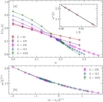
Figure 2: Determination of the critical point $\alpha_{c}$ with Binder cumulants and data collapse of order parameter. (a) Binder cumulants $U(\alpha,L)$ versus $\alpha$ for different system sizes. (Inset) The crossing point of $U(\alpha,L)$ with $U(\alpha,2L)$ versus $1/L$, from which the extrapolation $\alpha_{c}=2.2307(9)$ is determined. (b) Data collapse of the Néel order parameter close to $\alpha_{c}$, from which the optimised $\beta=0.57(2)$ and $\nu=2.16(1)$ are determined.

We first determine the critical point accurately by considering the Binder cumulants defined as $U=1-\frac{\langle m^{4}\rangle}{3\langle m^{2}\rangle^{2}}$, where $m=\frac{1}{N}\sum_{i=1}^{N}(-1)^{i}S_{i}^{z}$ is the Néel order parameter. The Binder cumulant is a dimensionless quantity, and according to the finite-size crossing point analysis [55], the crossing points ($\alpha^{*}(L)$) of $U(\alpha,L)$ and $U(\alpha,2L)$ is expected to converge to the phase transition point ($\alpha_{c}$) by $\alpha^{*}(L)=\alpha_{c}+L^{-b}$ [55, 56]. We thus measure the Binder cumulants for system sizes $L=64,128,256,512,1024$ and fix $\beta=L$ in the simulation. The crossing point is determined by fitting the data set with a cubic polynomial function and solving the intersection point of the fitted curves. This procedure is visible in Fig. 2 where panel (a) shows the Binder cumulant of the AF order for different system sizes as a function of $\alpha$. In the inset of Fig. 2 (a), from the extrapolation of power-law fitting of the crossing points to the thermodynamic limit, we obtain the critical point at $\alpha_{c}=2.2307(9)$, consistent and yet with higher accuracy compared with Refs. [2, 3, 4]. With such $\alpha_{c}$, we further collapse the AF order parameter $m^{2}$ to determine the critical exponents with the finite size scaling relation $m^{2}\cdot L^{2\beta/\nu}=f\left[(\alpha-\alpha_{c})\cdot L^{1/\nu}\right]$, where $\beta$ and $\nu$ are separately the critical exponents associated with order parameter and correlation length. As shown in Fig. 2 (b), we fix $\alpha_{c}=2.23$ and adjust the values of $\beta$ and $\nu$ to obtain the set of $(\beta,\nu)$ which collapse the data the best. Through this method, we obtain $\beta=0.57(2)$ and $\nu=2.16(1)$ are critical exponents at this transition point, which are consistent with Refs. [2, 3]. Together with the fact that the dynamic exponent $z<1$ [2, 4], this is a new quantum critical point distinct from conventional (1+1) dimensional QCPs, and we will study its nature through scaling of both EE and PE below.

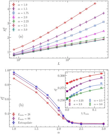
Figure 3: Unconventional scaling of the half-chain Rényi EE for ${\cal{H}}_{\rm LR}(\alpha)$ Eq. (1). (a) $S^{E}_{2}$ versus $L$ for different $\alpha$. (b) Extrapolation of fitted log-coefficient $\ell^{E}_{2}(\alpha)$ to the thermodynamic limit. In the analysis we gradually slide the fitting window which contains 6 data points for $\alpha>1$ and 5 data points for $\alpha=1$, and $L_{\text{min}}$ is the smallest system size in the fitting window. Inset exemplifies the finite-size and extrapolated $\ell^{E}_{2}(\alpha)$ for different $\alpha$ close to $\alpha_{c}$. For $\alpha>\alpha_{c}$, the system is described by a short-range (1+1)D CFT with $\ell^{E}_{2}(\alpha)=\frac{1}{4}$; for $\alpha\leq 1$, the system is in super LR regime with $\ell^{E}_{2}(\alpha)=1$. At $\alpha_{c}$, we find the $\ell^{E}_{2}(\alpha)=0.284(2)$ and it continuously increases in the long-range regime to $\ell^{E}_{2}(\alpha)=1$ in the super LR case.

Entanglement Entropy— The Rényi EE defined as $S_{n}^{E}=\frac{1}{1-n}\ln\operatorname{Tr}\rho_{A}^{n}$ ($\rho_{A}$ is the reduced density matrix of subsystem $A$), can be equivalently written as $S_{n}^{E}=\frac{1}{1-n}\ln\frac{Z_{A}^{(n)}}{Z^{(n)}}$ based on its trace structure [32, 33]. In SSE QMC’s configuration space [39], $Z_{A}^{(n)}$ can be represented as $n$ replicas of space-time configurations with region A glued together in imaginary time, and $Z^{(n)}$ represents n independent replicas. For a (1+1)d conformal field theory (CFT), if we fix region $A$ to be half of the chain, Rényi EE is analytically predicted to scale as [32]

$$S_{n}^{E}=\frac{c}{6}\left(1+\frac{1}{n}\right)\ln L+O(1),$$ (2)

where $c$ is the central charge of the CFT. For $\alpha>\alpha_{c}$, the LR interaction is irrelevant [2] so that we expect the EE to scale as Eq. (2). In the $n=2$ case, $S^{E}_{2}=\frac{c}{4}\ln L+O(1)$ with $c=1$ for short-range $SU(2)$ Heisenberg chain [57]. At the QCP $\alpha=\alpha_{c}$ and inside the LR regime $1<\alpha<\alpha_{c}$, the system is not described by a CFT, and the exact scaling of EE is not fully understood, despite very inspiring semi-classical results [30]. As detailed below, we find that our QMC data is perfectly described by the following logarithmic scaling

$$S^{E}_{2}=\ell^{E}_{2}(\alpha)\ln L+O(1),$$ (3)

with an unconventional $\alpha$-dependent coefficient $\ell^{E}_{2}(\alpha)$. In the LR regime where the system breaks SU$(2)$ symmetry, $\ell^{E}_{2}(\alpha)$ is finite, and continuously increases from $\ell^{E}_{2}(\alpha_{c})=0.284(2)$ to $\ell^{E}_{2}(\alpha=1)\to 1$. In the super-LR regime, the EE follows $S_{2}^{E}=\ln L+O(1)$, due to the tower of states (TOS) structure [58].

We thus compute the 2nd Rényi EE $S^{E}_{2}$ across the phase transition using the nonequilibrium increment method [46, 47, 48, 49] which is based on the Jarzynski’s equality [59] and overcome the fact that the EE is in general an exponential observable [60, 61]. This method makes use of a parameterized partition function interpolating between $Z_{A}^{(n)}$ and ${Z^{(n)}}$, and through tunning between the two partition functions the free energy difference can be calculated by accumulating the total work done during such tunning process [46, 47]. The Rényi entropy is thus obtained by relating itself with the free energy difference between $Z_{A}^{(n)}$ and ${Z^{(n)}}$. In practice, we use the increment trick [62] to accelerate this method [48, 49].

Fig. 3 (a) shows our results of EE for different $\alpha\in[1,\,3]$ at system size $L_{\text{max}}=540$ for $\alpha>1$, and $L_{\text{max}}=360$ for $\alpha=1$. As the system becomes more and more long-ranged, the finite-size effects manifest. We fit our results with Eq. (3) and fix the number of data points in fitting window to be 6. In this case, we gradually slide the fitting window and the smallest system size in the window is denoted by $L_{\text{min}}$. As exemplified in the inset of Fig. 3 (b), we use a quadratic function to fit the data points and extrapolate the log-coefficient $\ell^{E}_{2}(\alpha)$ to the thermodynamic limit ($1/L_{\text{min}}\rightarrow 0$). At the critical point, the data points extrapolate to $\ell^{E}_{2}(\alpha_{c})=0.284(2)$ which is intrinsically different from the SR CFT case $\alpha>\alpha_{c}$ with $\ell^{E}_{2}(\alpha)=0.25$. The main panel of Fig. 3 (b) thus shows the extrapolated $\ell^{E}_{2}(\alpha)$ with increasing $L_{\rm min}$ in the whole regime of $\alpha$. We observe that when $\alpha=1$, the extrapolated $\ell^{E}_{2}(\alpha)=0.970(3)$, close to the expectation of the super-LR regime, while the deviations can be attributed to strong finite-size effects at small $\alpha$. As $\alpha$ grows, $\ell^{E}_{2}(\alpha)$ gradually decreases and only gets to its CFT value $1/4$ when $\alpha>\alpha_{c}$. Note that close to $\alpha_{c}=2.23$ but in the SR regime, the extrapolation procedure yields a slightly larger value of $\ell^{E}_{2}(\alpha)$ than the expected $0.25$. We attribute this to strong finite-size effects to large correlation length in the critical regime. Besides the extrapolation shown in the inset of Fig. 3(b) for a few $\alpha$ values, the SM [63] shows extrapolation process of $\ell^{E}_{2}(\alpha)$ for the other $\alpha$.

Participation Entropy.— Another way to probe the quantum complexity of a many-body wavefunction is based on the participation entropy (PE), a quantity that has been shown to be very useful in capturing the universality of different quantum phases [34, 35, 36, 50, 51, 52, 53, 54, 64, 65, 66]. In short, for a given quantum state ${|\Psi\,\rangle}=\sum_{j}a_{j}{|j\,\rangle}$, expanded in a computational basis $\{|j\,\rangle\}$, one can naturally interpret $p_{j}=|a_{j}|^{2}$ as the probability to occupy the configuration $j$ by the normalized state ${|\Psi\,\rangle}$. One can then build the Rényi PEs (for a review, see [64]) defined as follows

$$S_{n}^{P}=\frac{1}{1-n}\ln\sum_{j}\left(p_{j}\right)^{n}.$$ (4)

Below, we only focus on the $n=\infty$ case, which is the easiest limit to handle with QMC since it only requires to record the most frequent basis state during the SSE sampling [54], yielding $S_{\infty}^{P}=-\ln p_{\rm max}$. For the AF model Eq. (1), the most probable spin configurations in the $\{S^{z}\}$ basis are the two (degenerate) Néel states: $|\hskip-2.84544pt\uparrow\downarrow\uparrow\downarrow\ldots\,\rangle$ and $|\hskip-2.84544pt\downarrow\uparrow\downarrow\uparrow\ldots\,\rangle$. It is remarkable that the knowledge of a single coefficient $p_{\rm max}$ (out of an exponentially large number) is sufficient to capture non-trivial quantum criticality  [34, 35, 36] or broken symmetry states [54, 67, 68].

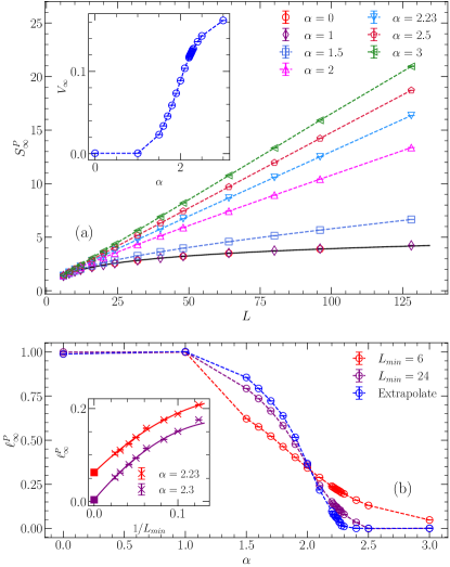
Figure 4: Unconventional scaling of the PE for ${\cal{H}}_{\rm LR}(\alpha)$ Eq. (1). (a) $S^{{P}}_{\infty}$ versus system size $L$ for different $\alpha$. Inset shows the extrapolated volume-law coefficient $V_{\alpha}$ for different $\alpha$. The solid black curve represents the relation of $S^{P}_{\infty}=\ln(L/2+1)$, which matches perfectly with finite-size PE data for both $\alpha=0$ and $\alpha=1$. (b) Extrapolation of fitted log-coefficient $\ell^{P}_{\infty}(\alpha)$ to the thermodynamic limit. In the analysis we gradually slide the fitting window which contains 5 data points for $\alpha\leq 1$ and 6 data points for other $\alpha$, and $L_{\text{min}}$ is the smallest system size in the fitting window. Inset shows the finite size extrapolation of log-coefficient $\ell^{P}_{\infty}(\alpha)$ for $\alpha_{c}$ and $\alpha=2.3$. $\ell^{P}_{\infty}(\alpha_{c})=0.065(2)$ yields an unconventional value for critical point and $\ell^{P}_{\infty}(\alpha=2.3)=0$ in the short-range regime.

For continuous symmetry breaking, the finite-size scaling of the PE has been first found to obey [54]

$$S_{\infty}^{P}(L)=V_{\infty}(\alpha)L+\ell^{P}_{\infty}(\alpha)\ln L+O(1),$$ (5)

with universal subleading logarithmic corrections such that $\ell^{P}_{\infty}(\alpha)$ directly depends on the number of linearly dispersing Nambu-Goldstone bosons $n_{\rm NG}$. The original conjecture $\ell^{P}_{\infty}(\alpha)=n_{\rm NG}/4$, made from high-precision QMC data on the 2D square lattice [54], was later shown analytically by Misguich, Pasquier and Oshikawa [67] who found two contributions of opposite signs, one (positive) coming form the TOS and the other (negative) from the spin-waves (SW). Below we aim at extending this to the peculiar case of broken continuous symmetry in $d=1$, with sublinear dispersing SW [23, 2, 30].

For this purpose, ${\cal{H}}_{\rm LR}(\alpha)$ Eq. (1) is very instructive, as it interpolates between two well-known limits. (i) In the SR regime for $\alpha>\alpha_{c}$, the Luttinger liquid (LL) behavior is expected [34, 50] with $S_{\infty}^{P}=V_{\infty}(\alpha)L-\ln\sqrt{K}+o(1)$, where $K$ is the LL parameter and $V_{\alpha}$ is a non-universal volume-law term that encodes the generic ground-state multifractality [51, 54]. (ii) The opposite limit $\alpha\to 0$ describes the fully connected Lieb-Mattis (LM) model [31], where the exact ground-state wave function is known [58], yielding $S_{\infty}^{P}=\ln\left(L/2+1\right)$ [54]. It is also natural to expect LM physics as soon as $\alpha<1$ [69]. On the other hand, in the long-range regime $1<\alpha<\alpha_{c}$ and at the QCP $\alpha_{c}$, we find that PE follows the unconventional scaling form of Eq. (5) with a continuously varying $\ell^{P}_{\infty}(\alpha)$.

Our results of $S_{\infty}^{P}(\alpha,L)$ are shown in Fig. 4. First, panel (a) clearly shows that in the super LR case for $\alpha=0,1$, QMC data follow the $S_{\infty}^{P}=\ln\left(L/2+1\right)$ behavior, with $V_{\infty}(\alpha)=0$ as denoted in the inset. Inside the LR regime and at the QCP, the generic scaling Eq. (5) is observed, with unconventional logarithmic corrections and varying $\ell^{P}_{\infty}(\alpha)$. Further increase $\alpha$ to $\alpha>\alpha_{c}$, the volume-law becomes dominant and the log-coefficient vanishes $\ell^{P}_{\infty}(\alpha)=0$, thus recovering the LL behavior. Fig. 4 (b) exhibits such evolution, the inset focusing on the log-coefficient close to $\alpha_{c}$. As $\alpha$ varies from 0 to large values, the log-coefficient $\ell^{P}_{\infty}(\alpha)$ in $S_{\infty}^{P}$ changes from 1 inside the super LR regime $\alpha\leq 1$, to a finite non-trivial value that should be related to the TOS and sublinear dispersing SW in the LR regime $1<\alpha<\alpha_{c}$. We remarkably observed a small but finite critical value $\ell^{P}_{\alpha=\alpha_{c}}\approx 0.065(2)$, which presumably jumps to 0 in the SR regime when $\alpha>\alpha_{c}$. The detailed fitting procedures are documented in the SM [63]. The existence of unconventional logarithmic correction to the PE, inside the long-range regime and at the QCP, further reinforces the consistent picture obtained from the scaling of EE in Fig. 3.

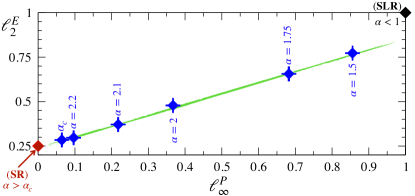
Figure 5: Linear dependence (the green line is a guide to the eyes) between $\ell^{P}_{\infty}(\alpha)$ and $\ell^{E}_{2}(\alpha)$ in the critical and LR regimes. In the SR regime, ($\ell^{P}_{\infty}=0,\ell^{E}_{2}=\frac{1}{4})$ as denoted by the red diamond. In the super-LR regime, ($\ell^{P}_{\infty}=1,\ell^{E}_{2}=1)$ as denoted by the black diamond.

Discussions.— We also find an interesting relation between the log-coefficients of the two entropies $\ell^{E}_{2}$ and $\ell^{P}_{\infty}$, as shown in Fig. 5. Starting from the SR regime where $\ell^{P}_{\infty}=0$ and $\ell^{E}_{2}=\frac{1}{4}$, the obtained estimates for $\ell^{P}_{\infty}(\alpha)$ and $\ell^{E}_{2}(\alpha)$ appear to be proportional, from $\alpha_{c}$ and through the entire LR regime, while inside the super-LR regime, $\ell^{P}_{\infty}=\ell^{E}_{2}=1$, deviating from the green line. It is tempting to interpret this observed linear dependence in the QCP and LR regimes as the result of a non-trivial combination of TOS and SW contributions [70, 71, 30, 67], but we leave this intriguing effect for further investigation.

To summarize, we have performed systematic finite size scaling of the entanglement entropy (EE) and participation entropy (PE) for long-range Heisenberg chain. We find distinctive scaling behaviors of both quantum entropies in the Super-LR $\alpha\leq 1$, LR $1<\alpha<\alpha_{c}\approx 2.23$, at the QCP $\alpha_{c}$ and inside the SR $\alpha>\alpha_{c}$ regimes. It is interesting that both entropies successfully reveal the unconventional logarithmic terms signifying the existence of the long-range order inside the LR regime, and at the QCP, separating the LR and SR regimes. The $\ell^{E}_{\alpha}$ and $\ell^{P}_{\infty}(\alpha)$ obtained also behave correctly inside the Super-LR and SR regimes where the analytic forms of EE and PE are known due to the fully connected Lieb-Mattis model [31] and exact knowledge of the ground state wavefunction of SU(2) Heisenberg chain with short-range interaction.

Our results and systematic analysis reveal that the quantum entanglement information, hidden in the finite size scaling of the two entropies employed here, can be obtained to the same level of order parameters and other usual finite size observables in the quantum many-body lattice models. We also foresee the experimental verification of our results, as quite remarkably, continuous symmetry breaking in spin chains with long-range interactions has recently been realized in trapped-ion quantum simulator [72].

Supplemental Material for
"Unconventional Scalings of Quantum Entropies in Long-Range Heisenberg Chains"

I Extrapolation of $\ell^{P}_{2}(\alpha)$ for different $\alpha$

Here in this section we show the extrapolation process of thermodynamic $\ell^{P}_{2}(\alpha)$ for different $\alpha$. In the analysis we gradually slide the fitting window which contains 6 data points for $\alpha>1.0$ and 5 data points for $\alpha=1.0$, and $L_{\text{min}}$ is the smallest system size in the fitting window. We extract the thermodynamic limit value of $\ell^{P}_{2}(\alpha)$ by fitting the finite size data points of $\ell^{P}_{2}(\alpha)(L_{\text{min}})$ to $1/L_{\text{min}=0}$ by fitting them with a quadratic function. As shown in Fig. S1, the extrapolated $\ell^{P}_{2}(\alpha)(L_{\text{min}}\rightarrow\infty)$ is denoted as a filled square and the finite size data points of $\ell^{P}_{2}(\alpha)(L_{\text{min}})$ are referred as empty circles.

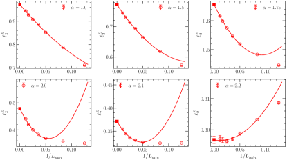
Figure S1: Extrapolation of thermodynamic $\ell^{P}_{2}(\alpha)$ with finite-size EE data for different $\alpha$. In the simulation we gradually slide the fitting window which contains 6 data points for $\alpha>1.0$ and 5 data points for $\alpha=1.0$, and $L_{\text{min}}$ is the smallest system size in the fitting window. The red curve is a fitting with of $\ell^{P}_{2}(\alpha)(L_{\text{min}})$ with a quadratic polynomial function. The solid filled square data point is the extrapolated thermodynamic $\ell^{P}_{2}(\alpha)$.

II Extrapolation of $\ell^{P}_{\infty}(\alpha)$ for different $\alpha$

Here in this section we show the extrapolation process of thermodynamic $\ell^{P}_{\infty}(\alpha)$ for different $\alpha$. In the analysis we gradually slide the fitting window which contains 6 data points for $\alpha>1.0$ and 5 data points for $\alpha=1.0$, and $L_{\text{min}}$ is the smallest system size in the fitting window. We extract the thermodynamic limit value of $\ell^{P}_{\infty}(\alpha)$ by fitting the finite size data points of $\ell^{P}_{2}(\alpha)(L_{\text{min}})$ to $1/L_{\text{min}=0}$ by fitting them with a quadratic function. As shown in Fig. S1, the extrapolated $\ell^{P}_{\infty}(\alpha)(L_{\text{min}}\rightarrow\infty)$ is denoted as a filled square and the finite size data points of $\ell^{P}_{\infty}(\alpha)(L_{\text{min}})$ are referred as empty circles. Note that for $\alpha\geq 2.3$ as shown in both Fig. 4 and S2, the extrapolated $\ell^{P}_{\infty}(\alpha)$ is negative, however we attribute this to strong finite-size effects. Actually, as shown in Fig. S3, after eliminating the volume term in PE by plotting $S^{{P}}_{\infty}(2L)-2S^{{P}}_{\infty}(L)$ against $\ln(L)$, at least when $\alpha\geq 2.28$, $S^{{P}}_{\infty}(2L)-2S^{{P}}_{\infty}(L)$ become flat and begins to grow as $L$ in increased. This shows that in the SR phase, $S^{{P}}_{\infty}(2L)-2S^{{P}}_{\infty}(L)$ is not linearly dependent on $\ln(L)$, but more likely to vary with $L$ due to finite size effects, consistent with our expectations. Furthermore, as in the short-range regime, $S_{\infty}^{P}=V_{\alpha}L-\ln\sqrt{K}+o(1)$ where $K$ is the LL parameters, we would expect as $L$ increases, $S^{{P}}_{\infty}(2L)-2S^{{P}}_{\infty}(L)$ will eventually converge to $\ln\sqrt{K}\sim-0.3466$. Our data for $\alpha=3.0$ clearly shows this tendency, although is still not converged. It is surely of great interest to push the system size to larger values to further examine this issue.

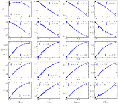
Figure S2: Extrapolation of thermodynamic $\ell^{P}_{\infty}(\alpha)$ with finite-size PE data for different $\alpha$. In the simulation we gradually slide the fitting window which contains 6 data points for $\alpha>1.0$ and 5 data points for $\alpha\leq 1.0$, and $L_{\text{min}}$ is the smallest system size in the fitting window. The red curve is a fitting with of $s$ with a quadratic polynomial function. The solid square filled data point is the extrapolated thermodynamic $\ell^{P}_{\infty}(\alpha)$.

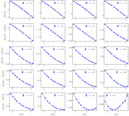
Figure S3: $S^{{P}}_{\infty}(2L)-2S^{{P}}_{\infty}(L)$ versus $\ln(L)$ for different $\alpha$ which cancels out the leading area law and exposes the logarithmic corrections (if any) as leading term of the scaling form..