Scaling of Disorder Operator and Entanglement Entropy at Easy-Plane Deconfined Quantum Criticalities
Abstract
We systematically investigate the scaling behavior of the disorder operator and the entanglement entropy (EE) of the easy-plane JQ (EPJQ) model at its transitions between the antiferromagnetic XY ordered phase (AFXY) and the valence bond solid (VBS) phase. We find (1) there exists a tiny yet finite value of the order parameters at the AFXY-VBS phase transition points of the EPJQ model, and the finite order parameter is strengthened as anisotropy varies from the Heisenberg limit () to the easy-plane limit (); (2) Both EE and disorder operator with smooth boundary cut exhibit anomalous scaling behavior at the transition points, resembling the scaling inside the Goldstone model phase, and the anomalous scaling becomes strengthened as the transition becomes more first order; (3) First put forward in Ref. [arXiv:2401.12838], with the finite-size corrections in EE for Goldstone phase is properly considered in the fitting form, the anomalous scaling behavior of EE can be adapted with emergent SO(5) symmetry breaking at the Heisenberg limit (). We extend this method in the EPJQ model and observe similar yet weaker results, which may indicate emergent SO(4) symmetry breaking in the easy-plane regime () or emergent SO(5) symmetry breaking in the Heisenberg limit (). These observations provide evidence that the Néel-VBS transition in the JQ model setting evolves from weak to prominent first-order transition as the system becomes anisotropic, and the non-local probes such as EE and disorder operator, serve as the sensitive tool to detect such salient yet fundamental features.
I Introduction
The conventional Landau-Ginzburg-Wilson (LGW) paradigm for characterizing phases and their transitions has been confronted with the notion of deconfined quantum critical points (DQCPs), which describes a direct continuous transition between Néel ordered phases and valence-bond-solid (VBS) phases Senthil (2004); Senthil et al. (2004); Levin and Senthil (2004); Senthil et al. (2005). However, the feasibility of realizing such transitions in lattice models remains a contentious issue because of the observations of various anomalous behavior against conformal field theories (CFT) Harada et al. (2013); Chen et al. (2013); Nahum et al. (2015); Nakayama and Ohtsuki (2016); Li (2022); Poland et al. (2019); Wang et al. (2022); Zhao et al. (2022a); Song et al. (2023a, b); Liu et al. (2023); Liao et al. (2023); Liu et al. (2024), such as drifting of critical exponents Harada et al. (2013); Chen et al. (2013); Nahum et al. (2015), violation of CFT bounds Nakayama and Ohtsuki (2016); Li (2022); Poland et al. (2019), and the anomalous scaling behavior of entanglement entropies and disorder operators Wang et al. (2022); Zhao et al. (2022a); Song et al. (2023a, b); Liu et al. (2023); Liao et al. (2023); Liu et al. (2024). A deeper exploration of the origins of these anomalous behaviors will benefit not only the better understanding of nature of DQCPs but also its lattice model and even material realizations Zayed et al. (2017); Guo et al. (2020); Jiménez et al. (2021); Sun et al. (2021); Cui et al. (2023); Guo et al. (2023).
Among all the anomalous behavior against CFTs, we are in particular interested in the anomalous finite-size scaling behavior of Rényi entanglement entropy (EE) and disorder operator, as it happens even at relatively small system sizes Wang et al. (2022); Zhao et al. (2022a); Song et al. (2023a, b); Liu et al. (2023); Liao et al. (2023); Liu et al. (2024) where other physical quantities such as order parameters and correlation functions still exhibit good agreement with a continuous phase transition Sandvik (2007); Lou et al. (2009); Shao et al. (2016); Ma et al. (2018a); Qin et al. (2017). In fact, at the DQCPs of SU(2) JQ2 and JQ3 models, our previous works Zhao et al. (2022a); Song et al. (2023a); Wang et al. (2022); Song et al. (2023b) show that disorder operator and EE all exhibit anomalous scaling against CFTs. To be specific, for the corner cut case where the boundary of subregion has four corners, both disorder operator and EE have a positive logarithmic correction to the leading order area law term which violates the unitary CFT prediction that the correction must be negative Casini and Huerta (2012); Fradkin and Moore (2006); Casini and Huerta (2007). Later, further studies clarified that the violation of EE actually arises from the smooth part of the subregion. In fact, for smooth cut case where the boundary has no sharp corners, the anomalous logarithmic subleading correction also exists in EE, which is incompatible with CFTs Song et al. (2023b, a), but seems to be more compatible with the existence of Goldstone modes Metlitski and Grover (2015); Deng et al. (2024) and can also possibly be adapted with the ‘walking" pseudo-criticality behavior at the transition Wang et al. (2017); Nahum (2020); Ma and Wang (2020); Zhou et al. (2023). In addition, recently another work D’Emidio and Sandvik (2024) shows that scaling of EE at the DQCP is cut-dependent, and the anomalous log correction for smooth cut can be suppressed by considering a tilted square lattice by degrees, and the essential information of the CFTs might be captured by this cut at small system sizes. In this context, the scalings of these nonlocal physical observables prove to be powerful and sensitive tools for diagnosing the various possible scenarios of the DQCPs Zhao et al. (2022a); Song et al. (2023a); Wang et al. (2022); Song et al. (2023b); Deng et al. (2024) and revealing the universal information of the possible CFT nearby the transitions D’Emidio and Sandvik (2024).
Here in this work, we aim to shed more insights on this issue by tunning the JQ-type Néel-VBS transition from weakly first-order to a more prominent first-order transition, such that many of the salient features observed at the SU(2) JQ limit, for example, the anomalous finite-size scaling behavior in the entanglement entropy (EE) Zhao et al. (2022a); Song et al. (2023a, b); Deng et al. (2024) and disorder operator Wang et al. (2022), can also be examined at a clear first-order transition, and the connection between the observed anomalous behavior in EE and disorder operator with the first-order nature of the transitions can be further clarified. A possible platform to achieve this goal is the easy-plane JQ (EPJQ) model, which adds the easy-plane anisotropy to the Heisenberg term in the JQ model, as shown in Eq. (1), to tune the Néel-VBS transition to be more first-ordered. Previous studies have investigated the nature of the Néel-VBS transition at different anisotropy , both in 2D and 3D lattice model settings Qin et al. (2017); Ma et al. (2019); Zhao et al. (2019); Desai and Kaul (2020); Sun et al. (2021), and the general expectation/observation is that the more tunes away from the Heisenberg limit () towards the easy-plane limit (), the stronger the first order of the Néel-VBS transition. The EPJQ model thus serves as an ideal platform to study the anomalous scaling behavior of EE and disorder operator at these transition points simply by tuning the values of .
In this paper, we use the stochastic series expansion (SSE) quantum Monte Carlo (QMC) methods Sandvik (1999); Syljuåsen and Sandvik (2002) to systematically study the order parameter, entanglement entropy, and disorder operator at the transitions of the EPJQ model. We carefully analyze the remaining ordered moments at the transitions and systematically study the evolution of the scaling of entanglement entropy and disorder operator along the critical line as a function of in Eq. (1). Our major findings are
-
1.
For there always exist tiny yet finite order parameters at the AFMXY/Néel-VBS phase transitions of the model (including the finite order parameter at the limit Takahashi et al. (2024)), indicating the first-order nature of the transition, and the moment increases as is tuned from 1 to 0;
-
2.
Both EE and disorder operator with standard smooth boundary cut (without tilting) exhibit anomalous scaling behavior against CFTs at the transition points, and resemble more to the scalings inside the Goldstone model phase, and the anomalous scalings also become strengthened as the transition becomes more first order;
-
3.
Pioneered in Ref. Deng et al. (2023a, 2024), with the finite-size corrections in EE for Goldstone phase is properly dealt with, the anomalous scaling behavior of EE can be adapted with emergent SO(5) symmetry breaking at the Heisenberg limit (). We extend this method in EPJQ model and observe similar yet weaker results which may indicate emergent SO(4) symmetry breaking in the easy-plane regime () or emergent SO(5) symmetry breaking in the Heisenberg limit ().
Our work thus provides a comprehensive study of the scaling of EE and disorder operator along the critical line where the weakly first-order transition is gradually tuned to a prominent first-order one by tunning to . We show that the anomalous scalings of EE and disorder operator are positively related with the first order behavior, proving a strong evidence that the DQCP of JQ model is indeed a very weakly-first-order transition and the anomalous log-corrections come from Goldstone modes. Apart from this, our work supports the findings in Ref. Deng et al. (2024) that the origin of anomalous scaling of EE at the transition of is the emergent continuous SO(5) symmetry breaking and the Goldstone modes associated with it. However, our results are weaker as we do not observe the same good convergence behavior to exact number of Goldstone modes required by the SO(5) symmetry breaking at or SO(4) symmetry breaking at , which might originate from insufficient data quality or the less pronounced emergent SO(4) symmetry behavior in the easy-plane case. Despite that, our results strongly suggest that the DQCPs of EPJQ model are first-ordered for all and scalings of EE and disorder operator serve as sensitive tools for detecting such transitions.
The rest of the paper is organized as follows. In Sec. II, we first introduce the EPJQ model and discuss how we extract the finite order parameters at its transition points, then we move on to the discussion of disorder operator in Sec. III and reveal its anomalous scaling with comparisons to that of the conventional (2+1)D O(3) QCP and Néel phase, next we discuss the results of EE at the EPJQ transitions in Sec. IV and point out its anomalous scaling very likely stems from the residual Goldstone mode at the first-order transition points, finally we give a comprehensive summary on our results, discuss the relation of our work with other recent works Deng et al. (2024); D’Emidio and Sandvik (2024) and point out future directions in Sec. V. Detailed analysis of the determination of the transition points and extrapolations of the order parameter, and the analysis of the quality of the fitting in EE data are presented in the Supplemental Material (SM) sup .
II Model and Phase Diagram
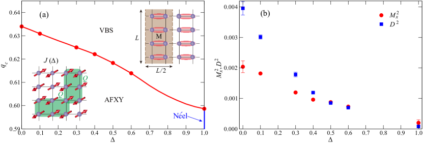
We study the easy-plane JQ3 (EPJQ) model Qin et al. (2017); Ma et al. (2019); Zhao et al. (2019); Desai and Kaul (2020); Sun et al. (2021) as illustrated in the lower left inset of Fig. 1 (a) with the following Hamiltonian
| (1) |
where is the two-spin singlet projector. For , the model reduces to JQ3 model with isotropic Heisenberg interactions. It has been found a direct quantum phase transition in the JQ3 model between the Néel and VBS phases happens at (with and as the energy unit) Lou et al. (2009); Wang et al. (2022). However, more numerical evidence, especially from the scaling of nonlocal observables such as EE Zhao et al. (2022a); Song et al. (2023a, b) and disorder operator Wang et al. (2022), reveal an anomalous behavior against CFTs even if the partitioning of the lattice is smooth, i.e. no sharp corners on the boundary. The fact that the sign of the observed log-coefficient is consistent with that of the presence of the Goldstone mode, further suggests there exist finite antiferromagnetic moment, i.e. remaining of the Néel order, at the transition point Metlitski and Grover (2015). Such evidence promotes the understanding that the Néel-VBS transition is indeed first order, despite being very weak at the SU(2) limit Takahashi et al. (2024). In this work, we monitor the behavior of both conventional order parameters and nonlocal observables at such transitions, as the anisotropy in Eq. (1) is tuned from the Heisenberg limit() to easy-plane limit ().
| 0.1 | 0.3 | 0.4 | 0.5 | 0.6 | ||
|---|---|---|---|---|---|---|
| using | 0.6340(1) | 0.63091(5) | 0.6250(2) | 0.6221(2) | 0.61833(6) | 0.6139(3) |
| using | 0.6341(5) | 0.6311(9) | 0.6261(4) | 0.6225(2) | 0.61883(5) | 0.6142(1) |
At each , the phase transition between the antiferromagnetic XY (AFXY) and VBS phase at zero temperature happens when tunning from zero to . To determine the critical points, we perform SSE-QMC simulations Sandvik (1999); Syljuåsen and Sandvik (2002) on the EPJQ model at for different system sizes with , , , and . In the AFXY phase, the order parameter is defined as the sublattice magnetization which breaks the U(1) symmetry, with the component being written as
| (2) |
where , are coordinates of site in the lattice. In the simulation with finite system sizes, the expectation value of can be viewed as the square of the AFXY order parameter, whereas at finite sizes.
For the VBS phase, the valence bonds can form in horizontal or vertical directions as exemplified of the former in the right inset of Fig. 1 (a). This order can be quantified through observables
| (3) |
with the coordinates of site . In this way, the expectation value of the square of the order parameter in VBS phase is .
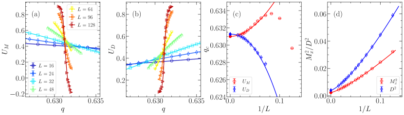
We thus perform the finite-size scaling (FSS) analysis of and to determine the transition points at the thermodynamic limit (TDL) Ma et al. (2018b). The dimensionless quantity Binder cumulants are widely used in the FSS to extract the critical points. For those two ground states in our study, the Binder cumulants are defined as
| (4) |
where normalization factors and constants in Eq. (4) are decided from the degree of freedom and number of components for order parameters. Under this definition, in AFXY while it is zero in the VBS state when . On the contrary, in AFXY phase and in the VBS phase. Besides, both and are dimensionless quantities whose value are independent of system sizes at critical points. In this way, for different simulated systems and at critical point , which means that the dependence of Binder cumulants for different sizes should cross with each other at the critical point.
Even though there only exist one phase transition point at thermodynamic limit (TDL) , usually all those curves will not exactly cross at because of the finite size effect and corrections. Therefore, we shall locate all the crossings where or and trace the using the following scaling form
| (5) |
with the correlation length exponent and the finite-size correction exponent Qin et al. (2017); Ma et al. (2018b); Chen et al. (2023).
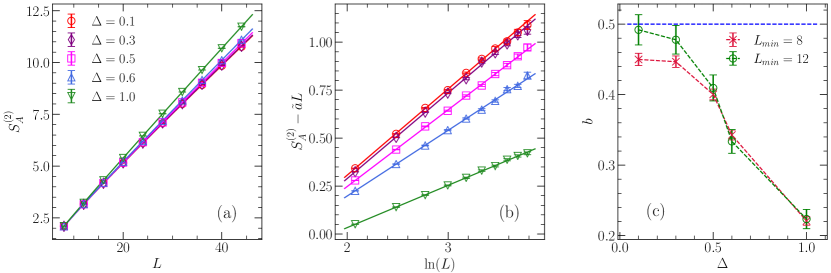
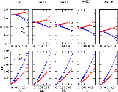
We perform such FSS analysis on the computed results in EPJQ model with different . For example, the Binder cumulants of both AFXY and VBS phases close to the crossing points are presented in Fig. 2 (a) and (b) for . The obtained crossings of two different curves with with increasing from to are then illustrated in Fig. 2 (c) as well as the fitting results. Using the fitting form in Eq. (5) two can be obtained with related to different order parameters. In Fig. 2 (d), we also present the extrapolation of the ordered moments (square) of and at each and eventually at the TDL, we find both and are finite (despite small in the -scale of the figure) at the transition point and this is the defining evidence that the transition is first-order.
Repeating such a procedure, we can also get for different in Tab. 1. For a given , the obtained from crossings of different dimensionless quantities agree with each other considering the error as large as two sigma, which can be true for the continuous phase transition as well as the first-order one. However, we should point out that of the AFXY order parameter for becomes negative close to at the largest simulated size , as shown in Fig. 2 (a), the negative can also be regarded as a signature of the first-order phase transition Binder and Landau (1984).
We have performed the extrapolation of the ordered moments as in Fig. 2 (d) for all the values, and the obtained results are summarized in Fig. 1 (b). It is clear that and are small at (they are even smaller at the isotropic limit), but they gradually increases as . We show all these extrapolations in the Sec. I of SM sup . The enhancement of the ordered moments as along the phase AFXY-VBS phase boundary in Fig. 1 (a) suggests evolution from very weakly first-order to stronger ones. As will be shown below, our non-local EE and disorder operator measurements (with smaller systems sizes compared with order parameters) can also capture such intriguing features.
For comparison, we have also studied the scaling of the disorder operator for the square lattice - Heisenberg model with the Hamiltonian
| (6) |
where denotes the bond and denotes the bond. This model has a well-established (2+1)d O(3) QCP at Ma et al. (2018b) separating the Néel phase and a symmetric singlet product phase. As will also shown below, the scaling of disorder operator of this O(3) QCP does not have anomalous log-corrections.
III Disorder Operator
Once the transition points of each are determined, we now carry out the analysis of the disorder operator upon them. As a non-local observable, disorder operator is defined as the expectation value of a symmetry transformation applied to a finite region in the statistical or quantum many-body systems of interest Wegner (1971); Kadanoff and Ceva (1971); Fradkin (2017); Nussinov and Ortiz (2009a, b). The design and implementation of the disorder operator and the analysis of its finite size scaling behavior have been successfully carried out in the situations of spontaneous symmetry breaking phase, quantum critical points, the symmetric phases with topological orders, symmetric mass generation transition and even the free fermion surface and interacting quantum critical Fermi surface systems Zhao et al. (2021); Wu et al. (2021a); Wang et al. (2021); Wu et al. (2021b); Chen et al. (2022); Wang et al. (2022); Jiang et al. (2023); Liu et al. (2023, 2024); Cai and Cheng (2024); Wu (2024).
In a 2D lattice spin model, for a region as shown in the right inset of Fig. 1 (a), we define the U(1) disorder operator , where is the U(1) charge on site . For the case of region M with sharp corners, the scaling of the U(1) disorder operator have been studied systematically Wu et al. (2021a); Wang et al. (2021); Wu et al. (2021b); Jiang et al. (2023). In the ordered (U(1) or SU(2) symmetry breaking) phases, such as the superfluid phase or Nel phase, it was found that Wang et al. (2021, 2022). At the quantum critical points of 2D lattice models, previous studies Zhao et al. (2021); Wang et al. (2021, 2022) showed that takes the following general form for a rectangle region :
| (7) |
where all the coefficients are functions of and the log-coefficient follows a universal function of both and the opening angles of the corners of ( for rectangle region). Given a smooth region M (without corners on boundary), there should be no corner correction and the log-coefficient . Such area-law decay of disorder operator, i.e. , holds both at the QCP and inside the gapped symmetric phases.
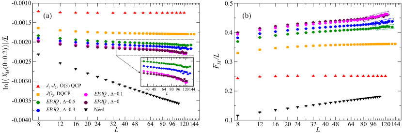
To detect the scaling of the disorder operator at the quantum phase transition point of EPJQ model in Eq. (1), we choose the entanglement region to be a cylinder region (without corners) in the lattice, as shown in the right inset of Fig. 1 (a), with system size for up to . For a good comparison between different quantum states, we calculated the U(1) disorder operator (with small rotation angle ) for the Néel phase (standard spin-1/2 Heisenberg model on the square lattice), the O(3) QCP of model in Eq. (6), DQCP of JQ3 model (Eq. (1) at ), and quantum phase transition points of EPJQ of Eq. (1) for , respectively. The results are shown in Fig. 3 (a).
As the leading term of the U(1) disorder operator at small for the Nel phase is , one expects proportional to with a pronounced slope, as shown in Fig. 3 (a). For the (2+1)D O(3) QCP of model, since with log-coefficient due to the smooth boundary, will be a constant at large system size, which is also clearly seen in Fig. 3 (a).
The case for the DQCP of JQ3 (), as a function of seems to be consistent with that of a normal quantum critical point, while for the corner cut case it has been found that the sign of log coefficient in Eq. 7 contradicts with unitary CFTs Wang et al. (2022). For the easy plane DQCPs (), one clearly sees that as is large enough there exist finite slopes and the slopes of became enhanced at the first-order phase transition points of EPJQ as anisotropy , as shown in the inset of Fig. 3 (a). Therefore, the scaling behavior of disorder operator resemble that of residual Nel orders, suggesting the first-order nature of the easy-plane DQCPs.
We have further computed a related quantity – the bipartite spin fluctuation Song et al. (2011). At limit, the scaling of the disorder operator has a similar behavior to that of the bipartite spin fluctuations, which is defined as
| (8) |
To be specific, at the Nel phase, the scaling of the bipartite fluctuations is Metlitski and Grover (2015); Song et al. (2011), and as show in Fig. 3 (b). For the (2+1)D O(3) QCP of model, the bipartite spin fluctuations of the smooth region have a linear scaling and will be a constant at large system size . For the DQCP of JQ3 model (), as a function of gives a tiny slope at large system size , suggesting a very tiny weakly first order nature of the transition point. More interestingly, the slopes of versus also become larger at the phase transition points of the EPJQ as decreases, especially at large system sizes and anisotropy as highlighted by dashed rectangular boxes of Fig. 3 (b). The scaling at large size reveals similar behavior as that of Nel orders contributed from the remaining Goldenstone mode. This finding further strengthens that the DQCP transitions change from weak to prominent first-order transitions from to .
IV Entanglement Entropy
Next we investigate the EE at the transition points of various of Eq. (1). To this end, we employ the nonequilibrium increment method Alba (2017); D’Emidio (2020); Zhao et al. (2022a, b) within the framework of SSE-QMC simulation Sandvik (1999); Syljuåsen and Sandvik (2002) to determine the second Rényi entropy of the EPJQ model at phase transition points for various values of . Rényi entanglement entropy is defined as which can be reexpressed in the form of according to the replica trick Calabrese and Cardy (2004). The nonequilibrium method is based on Jarzynski’s equality Jarzynski (1997), which relates the free energy difference between two systems with the total work done during a tuning process from one system to another. We regard the partition functions and as those of two different physical systems, then it is natural to apply the Jarzynski’s equality and design a tunning process between the two systems to calculate the Rényi entropies Alba (2017); D’Emidio (2020). In practice, we follow the incremental version Zhao et al. (2022a, b) of Ref. D’Emidio (2020), and it can overcome the obstacles that the EE is in general an exponential observable Zhang et al. (2024); Zhou et al. (2024). We conduct the simulation on a square lattice with periodic boundary conditions, and fix with and choose the subregion A to be a cylinder defined same as region in the right inset of Fig. 1 (a), which has no sharp corners on the entanglement boundary.
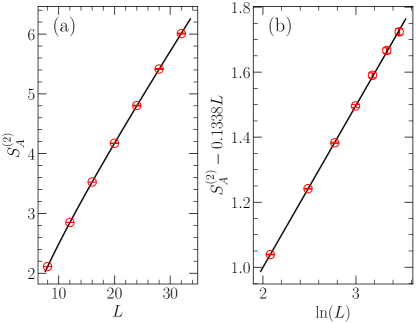
For , in the AFXY phase, the system spontaneously breaks the SO(2) spin symmetry and possesses one Goldstone mode. In this case, EE is expected to scale as Metlitski and Grover (2015)
| (9) |
where represents the number of Goldstone modes. Eq. (9) has been extensively verified for both XY phase with one Goldstone mode and Néel ordered states with two Goldstone modes respectively Helmes and Wessel (2014); Kulchytskyy et al. (2015); D’Emidio (2020); Zhao et al. (2022b); Song et al. (2023a); Deng et al. (2023b); Zhou et al. (2024); D’Emidio et al. (2024) . We first test our algorithm in the AFXY phase of the EPJQ model at and deep in the AFMXY phase, with the results displayed in Fig. 4. We measure the second order Rényi EE for the subsystem on a square lattice with smooth boundary. The system sizes utilized are and the temperature is fixed at . As shown in Fig. 4(b), by fitting the finite-size EE data to Eq. (9), we observe a good agreement between our data with the scaling form of Eq. (9). Moreover, the log-coefficient obtained from curve fitting is , aligning well with the expectation of existence of one Goldstone mode, which corresponds to spontaneous SO(2) symmetry breaking. The analysis of the fitting quality can be found in the Sec. II in SM sup .
We then proceed to the phase transition points. Our extrapolated finite order parameter data in Fig. 1(b) shows that the first-order behavior is more pronounced as decreases from 1 to 0. However, the relation between the scaling of entanglement entropy (EE) with the strengthen of first-order behavior remains unexplored. We measure the second Rényi EE at the transition points in Table. 1 for various values of and system sizes and fix . The subsystem A is again chosen to be cylinder withour corners on the boundary. As presented in Fig. 5, for all examined values of , we observe a clear logarithmic correction to the area law term in the scaling of EE (Eq. (9)). Additionally, as decreases and the first-order behavior strengthens, the fitted log-coefficient increases. Interestingly, for and , the fitted value of is even consistent with 0.5, which corresponds to the existence of a single Goldstone mode, the same as the scaling of EE deep inside the AFXY phase in Fig. 4. Our findings suggest that at least for the log-coefficient characterizes a evident first order transition with SO(2) symmetry breaking associated with one Goldstone mode.
At , where the system reduces to the isotropic JQ3 model, it has been discovered that even with a smooth entanglement boundary, the system exhibits anomalous positive logarithmic subleading corrections, resembling the Goldstone mode contribution, while the coefficient is only around 0.2-0.3 Song et al. (2023a, b). In addition, a recent study Deng et al. (2024) considers carefully the finite-size effects in scaling form for Goldstone mode phase, and apply the modified fitting function
| (10) |
where is the finite-size spin stiffness and the finite-size transverse spin susceptibility which are measured separately in QMC simulations and substituted in the above relation to fit the finite-size EE data. Through this procedure, the log-coefficient is fitted to be around 2 which corresponds to four Goldstone modes Deng et al. (2024). This is used to suggest that the system breaks the emergent SO(5) symmetry at the transition point, and this process can be well detected by the scaling of EE even at relatively small system sizes Deng et al. (2024).
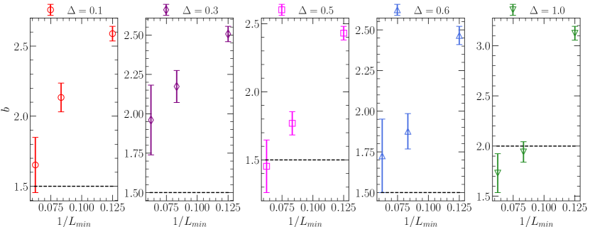
We followed this procedure, calculated the finite-size spin stiffness and transverse spin susceptibility , and substituted them in Eq. (10), same as in Ref. Deng et al. (2024) to fit our EE data. However, as shown in Fig. 6, we find it is difficult to observe the same convergence of log-coefficient to 2 at or to 1.5 at , which would suggest the breaking of emergent SO(5) (four Goldstone modes) and SO(4) (three Goldstone modes) symmetries, respectively. In fact, at the last two data points with larger are quite close to , although the last data point slightly deviates below .
For , except for , the last data points all seem to be consistent with . However, within our limited data quality, we do not observe the stability of fitted results with respect to for any . It is possible that our results can be affected by stronger finite-size effects as we fixed to approach the thermodynamic limit, while Ref. Deng et al. (2024) used the projector quantum Monte Carlo Sandvik (2010, 2005) to simulate the ground state of the system and fix the projection power to be . Another possible explanation is, as we observed at the first order is enhanced, the emergent behavior can be weakened and broken into remaining VBS order and Goldstone phase at small system sizes. In this case, within the system sizes we considered, an evident first-order behavior with only one Goldstone mode might be mixed with the symmetry breaking behavior with three Goldstone modes. Then the fitted log coefficient with Eq. (10) for could drift significantly from 1.5 to 0.5 as system sizes grow. Therefore our fitting results with Eq. (10) are consistent with Ref. Deng et al. (2024) for JQ3 model and show the capability of EE in characterizing the emergent symmetry and weakly first order behaviors at the complicated DQCPs.
V Discussion
Our work shows the two non-local measurements – the disorder operator and entanglement entropy – consistently exhibit anomalous scaling behaviors at the easy-plane deconfined quantum criticalities. By adjusting the anisotropy from the Heisenberg limit () to the easy-plane limit (), we find that as the first-order nature of the transition is amplified, the anomalous behavior for both disorder operator and entanglement entropy becomes more apparent, resembling contributions from Goldstone modes. Interestingly, when , the log coefficient in EE seem to converge to which is consistent with one Goldstone mode and SO(2) symmetry breaking at the first-order transition points. Additionally, when applying the finite-size fitting form of Goldstone mode phase (Eq. (10)) to fit our EE data, we obtain the enhanced log coefficients close to that of emergent SO(5) symmetry breaking at and emergent SO(4) symmetry breaking at . However, the log coefficients do not show the good convergence behavior, as shown in Ref. Deng et al. (2024), which maybe explained by insufficient data quality or very weak emergent SO(4) symmetry at due to the strengthening of first order behavior. Our work thus provides strong evidence that the observed anomalous scaling behaviors of the entanglement measurements (disorder operator and EE) indeed come from the weakly-first-order nature of DQCPs of JQ model realizations both at and .
Note that our work and previous studies Wang et al. (2022); Zhao et al. (2022a); Song et al. (2023a, b); Liu et al. (2023); Liao et al. (2023); Liu et al. (2024); D’Emidio and Sandvik (2024); Deng et al. (2024) on the EE scaling of smooth cut on a square lattice are not contradicted with the recent work by D’Emidio and Sandvik D’Emidio and Sandvik (2024) where they consider a -degrees-tilted square lattice and observe the normal scaling of EE obeying the requirements of CFTs. On the contrary, the cut dependence of EE might support the transition is indeed weakly-first order and the tilted cut and standard cut possibly just capture the two sides of the JQ-type DQCP story. On the one hand, it is a weakly first transition which can be detected by the standard cut, and on the other hand the system might be close to a real continuous transition so that the tilted cut captures some essential information of the CFT at small system sizes. In conclusion, scaling of these nonlocal observables have proven to be both powerful and sensitive tools in characterising this kind of weakly first-order transitions Wang et al. (2022); Zhao et al. (2022a); Song et al. (2023a); Deng et al. (2024), and it provides strong evidence that the JQ type DQCP is weakly first order however very close to a real continuous transition Takahashi et al. (2024), possibly of multicritical type related with the SO(5) model with Wess-Zumino-Witten term Zhao et al. (2020); Chen et al. (2023); Chester and Su (2024); Takahashi et al. (2024); Chen et al. (2024) or the ‘walking" pseudo-criticality behavior at the transition Wang et al. (2017); Nahum (2020); Ma and Wang (2020); Zhou et al. (2023).
Future research directions may include investigating the disorder operator and entanglement entropy scaling of JQn models with , which have been shown to exhibit stronger first-order transitions Takahashi and Sandvik (2020); Takahashi et al. (2024) as increases, similar to EPJQ models. Another avenue of interest is to explore the entanglement entropy scaling of an absolutely strong first-order transition, which involves a mixture of two phases with classical probabilities. Moreover, multipartite entanglement Osborne and Nielsen (2002); Javanmard et al. (2018); Wang et al. (2024); Parez and Witczak-Krempa (2024) and higher-order Rényi entropies, entanglement negativity and entanglement spectrum Wu et al. (2020); Wang and Xu (2023); Yan and Meng (2023) with QMC simulations at the DQCP also present intriguing topics for future investigation.
Acknowledgement
We thank Meng Cheng, Cenke Xu, Anders Sandvik, Senthil Todadri, Subir Sachdev for valuable discussions on the related topic. NVM and ZYM acknowledge the earlier insightful discussions on the transitions of EPJQ model with Arnab Sen and Anders Sandvik. JRZ and ZYM acknowledge the support from the Research Grants Council (RGC) of Hong Kong Special Administrative Region of China (Project Nos. 17301721, AoE/P-701/20, 17309822, HKU C7037- 22GF, 17302223), the ANR/RGC Joint Research Scheme sponsored by RGC of Hong Kong and French National Research Agency (Project No. A HKU703/22), the GD-NSF (No. 2022A1515011007) and the HKU Seed Funding for Strategic Interdisciplinary Research. Y.C.W. acknowledges the support from Zhejiang Provincial Natural Science Foundation of China (Grant No. LZ23A040003), and the support from the High-Performance Computing Centre of Hangzhou International Innovation Institute of Beihang University. NVM acknowledge the National Natural Science Foundation of China (No. 12004020) and the Fundamental Research Funds for the Central Universities. We thank HPC2021 system under the Information Technology Services and the Blackbody HPC system at the Department of Physics, University of Hong Kong, as well as the Beijng PARATERA Tech CO.,Ltd. (URL: https://cloud.paratera.com) for providing HPC resources that have contributed to the research results reported within this paper.
References
- Senthil (2004) T. Senthil, Science 303, 1490–1494 (2004).
- Senthil et al. (2004) T. Senthil, L. Balents, S. Sachdev, A. Vishwanath, and M. P. A. Fisher, Phys. Rev. B 70, 144407 (2004).
- Levin and Senthil (2004) M. Levin and T. Senthil, Physical Review B 70, 220403 (2004).
- Senthil et al. (2005) T. Senthil, L. Balents, S. Sachdev, A. Vishwanath, and M. P. A. Fisher, Journal of the Physical Society of Japan 74, 1 (2005), https://doi.org/10.1143/JPSJS.74S.1 .
- Harada et al. (2013) K. Harada, T. Suzuki, T. Okubo, H. Matsuo, J. Lou, H. Watanabe, S. Todo, and N. Kawashima, Physical Review B 88, 220408 (2013).
- Chen et al. (2013) K. Chen, Y. Huang, Y. Deng, A. B. Kuklov, N. V. Prokof’ev, and B. V. Svistunov, Phys. Rev. Lett. 110, 185701 (2013).
- Nahum et al. (2015) A. Nahum, J. Chalker, P. Serna, M. Ortuño, and A. Somoza, Physical Review X 5, 041048 (2015).
- Nakayama and Ohtsuki (2016) Y. Nakayama and T. Ohtsuki, Phys. Rev. Lett. 117, 131601 (2016).
- Li (2022) Z. Li, JHEP 11, 005 (2022), arXiv:1812.09281 [hep-th] .
- Poland et al. (2019) D. Poland, S. Rychkov, and A. Vichi, Rev. Mod. Phys. 91, 015002 (2019).
- Wang et al. (2022) Y.-C. Wang, N. Ma, M. Cheng, and Z. Y. Meng, SciPost Phys. 13, 123 (2022).
- Zhao et al. (2022a) J. Zhao, Y.-C. Wang, Z. Yan, M. Cheng, and Z. Y. Meng, Phys. Rev. Lett. 128, 010601 (2022a).
- Song et al. (2023a) M. Song, J. Zhao, Z. Y. Meng, C. Xu, and M. Cheng, arXiv e-prints , arXiv:2312.13498 (2023a), arXiv:2312.13498 [cond-mat.str-el] .
- Song et al. (2023b) M. Song, J. Zhao, M. Cheng, C. Xu, M. M. Scherer, L. Janssen, and Z. Y. Meng, arXiv e-prints , arXiv:2307.02547 (2023b), arXiv:2307.02547 [cond-mat.str-el] .
- Liu et al. (2023) Z. H. Liu, W. Jiang, B.-B. Chen, J. Rong, M. Cheng, K. Sun, Z. Y. Meng, and F. F. Assaad, Phys. Rev. Lett. 130, 266501 (2023).
- Liao et al. (2023) Y. D. Liao, G. Pan, W. Jiang, Y. Qi, and Z. Y. Meng, arXiv e-prints , arXiv:2302.11742 (2023), arXiv:2302.11742 [cond-mat.str-el] .
- Liu et al. (2024) Z. H. Liu, Y. Da Liao, G. Pan, M. Song, J. Zhao, W. Jiang, C.-M. Jian, Y.-Z. You, F. F. Assaad, Z. Y. Meng, and C. Xu, Phys. Rev. Lett. 132, 156503 (2024).
- Zayed et al. (2017) M. Zayed, C. Rüegg, J. Larrea J, A. Läuchli, C. Panagopoulos, S. Saxena, M. Ellerby, D. McMorrow, T. Strässle, S. Klotz, G. Hamel, R. A. Sadykov, V. Pomjakushin, M. Boehm, M. Jiménez–Ruiz, A. Schneidewind, E. Pomjakushina, M. Stingaciu, C. K., and H. M. Rønnow, Nature physics 13, 962 (2017).
- Guo et al. (2020) J. Guo, G. Sun, B. Zhao, L. Wang, W. Hong, V. A. Sidorov, N. Ma, Q. Wu, S. Li, Z. Y. Meng, A. W. Sandvik, and L. Sun, Phys. Rev. Lett. 124, 206602 (2020).
- Jiménez et al. (2021) J. L. Jiménez, S. P. G. Crone, E. Fogh, M. E. Zayed, R. Lortz, E. Pomjakushina, K. Conder, A. M. Läuchli, L. Weber, S. Wessel, A. Honecker, B. Normand, C. Rüegg, P. Corboz, H. M. Rønnow, and F. Mila, Nature 592, 370 (2021).
- Sun et al. (2021) G. Sun, N. Ma, B. Zhao, A. W. Sandvik, and Z. Y. Meng, Chinese Physics B 30, 067505 (2021).
- Cui et al. (2023) Y. Cui, L. Liu, H. Lin, K.-H. Wu, W. Hong, X. Liu, C. Li, Z. Hu, N. Xi, S. Li, R. Yu, A. W. Sandvik, and W. Yu, Science 380, 1179 (2023).
- Guo et al. (2023) J. Guo, P. Wang, C. Huang, B.-B. Chen, W. Hong, S. Cai, J. Zhao, J. Han, X. Chen, Y. Zhou, S. Li, Q. Wu, Z. Y. Meng, and L. Sun, arXiv e-prints , arXiv:2310.20128 (2023), arXiv:2310.20128 [cond-mat.str-el] .
- Sandvik (2007) A. W. Sandvik, Phys. Rev. Lett. 98, 227202 (2007).
- Lou et al. (2009) J. Lou, A. W. Sandvik, and N. Kawashima, Phys. Rev. B 80, 180414 (2009).
- Shao et al. (2016) H. Shao, W. Guo, and A. W. Sandvik, Science 352, 213 (2016).
- Ma et al. (2018a) N. Ma, G.-Y. Sun, Y.-Z. You, C. Xu, A. Vishwanath, A. W. Sandvik, and Z. Y. Meng, Phys. Rev. B 98, 174421 (2018a).
- Qin et al. (2017) Y. Q. Qin, Y.-Y. He, Y.-Z. You, Z.-Y. Lu, A. Sen, A. W. Sandvik, C. Xu, and Z. Y. Meng, Phys. Rev. X 7, 031052 (2017).
- Casini and Huerta (2012) H. Casini and M. Huerta, Journal of High Energy Physics 2012, 87 (2012).
- Fradkin and Moore (2006) E. Fradkin and J. E. Moore, Phys. Rev. Lett. 97, 050404 (2006).
- Casini and Huerta (2007) H. Casini and M. Huerta, Nucl. Phys. B 764, 183–201 (2007).
- Metlitski and Grover (2015) M. A. Metlitski and T. Grover, (2015), arXiv:1112.5166 [cond-mat.str-el] .
- Deng et al. (2024) Z. Deng, L. Liu, W. Guo, and H.-q. Lin, arXiv e-prints , arXiv:2401.12838 (2024), arXiv:2401.12838 [cond-mat.str-el] .
- Wang et al. (2017) C. Wang, A. Nahum, M. A. Metlitski, C. Xu, and T. Senthil, Physical Review X 7, 031051 (2017).
- Nahum (2020) A. Nahum, Phys. Rev. B 102, 201116 (2020).
- Ma and Wang (2020) R. Ma and C. Wang, Phys. Rev. B 102, 020407 (2020).
- Zhou et al. (2023) Z. Zhou, L. Hu, W. Zhu, and Y.-C. He, arXiv preprint arXiv:2306.16435 (2023).
- D’Emidio and Sandvik (2024) J. D’Emidio and A. W. Sandvik, arXiv e-prints , arXiv:2401.14396 (2024), arXiv:2401.14396 [cond-mat.str-el] .
- Ma et al. (2019) N. Ma, Y.-Z. You, and Z. Y. Meng, Phys. Rev. Lett. 122, 175701 (2019).
- Zhao et al. (2019) B. Zhao, P. Weinberg, and A. W. Sandvik, Nature Physics 15, 678 (2019).
- Desai and Kaul (2020) N. Desai and R. K. Kaul, Phys. Rev. B 102, 195135 (2020).
- Sandvik (1999) A. W. Sandvik, Phys. Rev. B 59, R14157 (1999).
- Syljuåsen and Sandvik (2002) O. F. Syljuåsen and A. W. Sandvik, Phys. Rev. E 66, 046701 (2002).
- Takahashi et al. (2024) J. Takahashi, H. Shao, B. Zhao, W. Guo, and A. W. Sandvik, arXiv e-prints , arXiv:2405.06607 (2024), arXiv:2405.06607 [cond-mat.str-el] .
- Deng et al. (2023a) Z. Deng, L. Liu, W. Guo, and H. Q. Lin, Phys. Rev. B 108, 125144 (2023a).
- (46) Determination of the transition points and extrapolations of the order parameters, and the analysis of the quality of the fitting in EE data are presented in this Supplemental Material .
- Ma et al. (2018b) N. Ma, P. Weinberg, H. Shao, W. Guo, D.-X. Yao, and A. W. Sandvik, Phys. Rev. Lett. 121, 117202 (2018b).
- Chen et al. (2023) B.-B. Chen, X. Zhang, Y. Wang, K. Sun, and Z. Y. Meng, arXiv e-prints , arXiv:2307.05307 (2023), arXiv:2307.05307 [cond-mat.str-el] .
- Binder and Landau (1984) K. Binder and D. P. Landau, Phys. Rev. B 30, 1477 (1984).
- Wegner (1971) F. Wegner, J. Math. Phys. 12, 2259 (1971).
- Kadanoff and Ceva (1971) L. P. Kadanoff and H. Ceva, Phys. Rev. B 3, 3918 (1971).
- Fradkin (2017) E. Fradkin, Journal of Statistical Physics 167, 427 (2017).
- Nussinov and Ortiz (2009a) Z. Nussinov and G. Ortiz, Proceedings of the National Academy of Sciences 106, 16944 (2009a).
- Nussinov and Ortiz (2009b) Z. Nussinov and G. Ortiz, Annals of Physics 324, 977 (2009b).
- Zhao et al. (2021) J. Zhao, Z. Yan, M. Cheng, and Z. Y. Meng, Phys. Rev. Res. 3, 033024 (2021).
- Wu et al. (2021a) X.-C. Wu, W. Ji, and C. Xu, Journal of Statistical Mechanics: Theory and Experiment 2021, 073101 (2021a).
- Wang et al. (2021) Y.-C. Wang, M. Cheng, and Z. Y. Meng, Phys. Rev. B 104, L081109 (2021).
- Wu et al. (2021b) X.-C. Wu, C.-M. Jian, and C. Xu, SciPost Phys. 11, 033 (2021b).
- Chen et al. (2022) B.-B. Chen, H.-H. Tu, Z. Y. Meng, and M. Cheng, Phys. Rev. B 106, 094415 (2022).
- Jiang et al. (2023) W. Jiang, B.-B. Chen, Z. H. Liu, J. Rong, F. F. Assaad, M. Cheng, K. Sun, and Z. Y. Meng, SciPost Phys. 15, 082 (2023).
- Cai and Cheng (2024) K.-L. Cai and M. Cheng, arXiv e-prints , arXiv:2404.04334 (2024), arXiv:2404.04334 [cond-mat.str-el] .
- Wu (2024) X.-C. Wu, arXiv e-prints , arXiv:2404.04331 (2024), arXiv:2404.04331 [cond-mat.str-el] .
- Song et al. (2011) H. F. Song, N. Laflorencie, S. Rachel, and K. Le Hur, Phys. Rev. B 83, 224410 (2011).
- Alba (2017) V. Alba, Phys. Rev. E 95, 062132 (2017).
- D’Emidio (2020) J. D’Emidio, Phys. Rev. Lett. 124, 110602 (2020).
- Zhao et al. (2022b) J. Zhao, B.-B. Chen, Y.-C. Wang, Z. Yan, M. Cheng, and Z. Y. Meng, npj Quantum Materials 7, 69 (2022b).
- Calabrese and Cardy (2004) P. Calabrese and J. Cardy, Journal of Statistical Mechanics: Theory and Experiment 2004, P06002 (2004).
- Jarzynski (1997) C. Jarzynski, Phys. Rev. Lett. 78, 2690 (1997).
- Zhang et al. (2024) X. Zhang, G. Pan, B.-B. Chen, K. Sun, and Z. Y. Meng, Phys. Rev. B 109, 205147 (2024).
- Zhou et al. (2024) X. Zhou, Z. Y. Meng, Y. Qi, and Y. Da Liao, Phys. Rev. B 109, 165106 (2024).
- Helmes and Wessel (2014) J. Helmes and S. Wessel, Phys. Rev. B 89, 245120 (2014).
- Kulchytskyy et al. (2015) B. Kulchytskyy, C. M. Herdman, S. Inglis, and R. G. Melko, Phys. Rev. B 92, 115146 (2015).
- Deng et al. (2023b) Z. Deng, L. Liu, W. Guo, and H. Q. Lin, Phys. Rev. B 108, 125144 (2023b).
- D’Emidio et al. (2024) J. D’Emidio, R. Orús, N. Laflorencie, and F. de Juan, Phys. Rev. Lett. 132, 076502 (2024).
- Sandvik (2010) A. W. Sandvik, AIP Conference Proceedings 1297, 135 (2010), https://aip.scitation.org/doi/pdf/10.1063/1.3518900 .
- Sandvik (2005) A. W. Sandvik, Phys. Rev. Lett. 95, 207203 (2005).
- Zhao et al. (2020) B. Zhao, J. Takahashi, and A. W. Sandvik, Phys. Rev. Lett. 125, 257204 (2020).
- Chester and Su (2024) S. M. Chester and N. Su, Phys. Rev. Lett. 132, 111601 (2024).
- Chen et al. (2024) B.-B. Chen, X. Zhang, and Z. Y. Meng, arXiv e-prints , arXiv:2405.04470 (2024), arXiv:2405.04470 [cond-mat.str-el] .
- Takahashi and Sandvik (2020) J. Takahashi and A. W. Sandvik, Phys. Rev. Res. 2, 033459 (2020).
- Osborne and Nielsen (2002) T. J. Osborne and M. A. Nielsen, Phys. Rev. A 66, 032110 (2002).
- Javanmard et al. (2018) Y. Javanmard, D. Trapin, S. Bera, J. H. Bardarson, and M. Heyl, New Journal of Physics 20, 083032 (2018).
- Wang et al. (2024) T.-T. Wang, M. Song, L. Lyu, W. Witczak-Krempa, and Z. Y. Meng, arXiv e-prints , arXiv:2402.14916 (2024), arXiv:2402.14916 [cond-mat.str-el] .
- Parez and Witczak-Krempa (2024) G. Parez and W. Witczak-Krempa, arXiv e-prints , arXiv:2402.06677 (2024), arXiv:2402.06677 [quant-ph] .
- Wu et al. (2020) K.-H. Wu, T.-C. Lu, C.-M. Chung, Y.-J. Kao, and T. Grover, Phys. Rev. Lett. 125, 140603 (2020).
- Wang and Xu (2023) F.-H. Wang and X. Y. Xu, arXiv e-prints , arXiv:2312.14155 (2023), arXiv:2312.14155 [cond-mat.str-el] .
- Yan and Meng (2023) Z. Yan and Z. Y. Meng, Nature Communications 14, 2360 (2023).
Supplemental Material for
"Scaling of Disorder Operator and Entanglement Entropy at Easy-Plane Deconfined Quantum Criticalities"
I The criticality for different in the EPJQ models
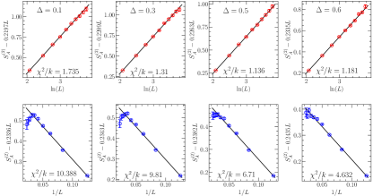
The results in (b) of Fig. 1 in the main text present that the order parameters for both the AFXY and VBS phases converge to a non-zero value when goes to infinity for different in the EPJQ models, which implies the possibility of first-order phase transitions in the EPJQ model. In this section we present the detail procedure in obtaining those converged order parameters at thermodynamic limit in Fig. 1(b). The binder cumulants and defined in Eq. (4) for the AFXY and VBS phases correspondingly are two dimensionless quantities that are commonly chosen in the FSS of calculating critical points and correlation length exponents. In this paper we study the critical behavior of the EPJQ model with different anisotropic value with the help of and all the crossing points of two simulated sizes and got from and are shown in the first row in Fig. S1 for those different . Using the fitting form in Eq. (5) two can be got, which are listed in Tab.1 in the main text. At each crossing point we also calculate the square of order parameters defined in Eq. 2 and Eq. 3 as and illustated in the second row in Fig. S1. It should be noticed that and are calculated at different as the crossing points are got from different dimensionless quantities. In the calculation of we chose the corresponding got from for two sizes and . As for the the crossing points are located using . After all the and are known for different sizes, the square of order parameters at critical points when can be calculated with the second-order polynomial fitting. All the fitting parameters of and for different are illustrated in Fig. 1 in the main text.
II Comparison of fitting quality
In the main text, the scaling form of EE we use for the fitting is
| (S1) |
However, to confirm the validity of the fitting form we use, we consider the comparison of above fitting form with the following one
| (S2) |
which has no subleading dependence term but with a finite-size correction term .
We use the chi-squared value to evaluate the fitting quality. chi-squared value is defined as
| (S3) |
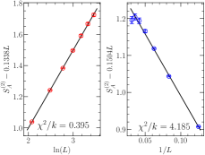
where is the uncertainty of data . is the effective number of degrees of freedom, where is the number of data points and is the number of fitting parameters. is expected to be close to 1 for a good fit. As shown in Fig. S2, in the AFMXY phase, the fitting quality is compared with Eq. S1 and Eq. S2 and the values are 0.395 and 4.185 separately. should be typically distributed within the range where for this case the range is . In our simulation, the precise estimation of statistic errors can be affected by limited number of Monte Carlo bins so that we attribute the small deviation of 0.395 to 0.465 to problematic errorbars and 4.185 is apparently far away from the ideal range. We thus conclude that Eq. S1 fits the data better than Eq. S2.
Similarly, for DQCPs of easy-plane model, the comparison of fitting quality with Eq. S1 and Eq. S2 is also performed and the results are shown in Fig. S3. By comparing their values, we conclude that Eq. S1 in all cases fit better than Eq. S2. Note that for which is the standard model, it has already been shown in previous study Song et al. (2023a) that Eq. S1 fits the better. In that case we only present the comparison for in this manuscript.