Physics Department, Technion, 32000 Haifa, Israel.
Quantum Transport Theory of Strongly Correlated Matter
Abstract
This report reviews recent progress in computing Kubo formulas for general interacting Hamiltonians. The aim is to calculate electric and thermal magneto-conductivities in strong scattering regimes where Boltzmann equation and Hall conductivity proxies exceed their validity. Three primary approaches are explained.
-
1.
Degeneracy-projected polarization formulas for Hall-type conductivities, which substantially reduce the number of calculated current matrix elements. These expressions generalize the Berry curvature integral formulas to imperfect lattices.
-
2.
Continued fraction representation of dynamical longitudinal conductivities. The calculations produce a set of thermodynamic averages, which can be controllably extrapolated using their mathematical relations to low and high frequency conductivity asymptotics.
-
3.
Hall-type coefficients summation formulas, which are constructed from thermodynamic averages.
The thermodynamic formulas are derived in the operator Hilbert space formalism, which avoids the opacity and high computational cost of the Hamiltonian eigenspectrum. The coefficients can be obtained by well established imaginary-time Monte Carlo sampling, high temperature expansion, traces of operator products, and variational wavefunctions at low temperatures.
We demonstrate the power of approaches 1–3 by their application to well known models of lattice electrons and bosons. The calculations clarify the far-reaching influence of strong local interactions on the metallic transport near Mott insulators. Future directions for these approaches are discussed.
Part I Introduction
1 Why calculate conductivities?
Theorists commonly describe phases of matter by their order parameters, since they can be calculated by tried and tested algorithms of equilibrium statistical mechanics. These “thermodynamic methods” include stochastic series expansions [1], worm algorithm of Quantum Monte-Carlo simulations [2], and variational methods such as density matrix renormalization group [3, 4], projected entangled-pair states [5] and tensor networks [6].
Experimentalists on the other hand, commonly probe phases of matter by transport measurements. For example: Hall coefficients can characterize the current-carriers’ density (near band extrema). Temperature dependent resistivity may herald the onset of superconductivity or charge localization. Quantized Hall conductivity is associated with topologically ordered ground states.
Electric, thermo-electric and thermal transport coefficients, and , are defined by linear response equations,
| (1) |
and are the electric and thermal currents respectively. and are the electrochemical field and temperature gradient respectively. In Eq. (1), the wavevector and frequency dependence of all variables are suppressed.
For systems described by weakly scattered Bloch-band quasiparticles, the Boltzmann equation [7, 8] and diagrammatic perturbation theory [9] are adequate. For incompressible quantum Hall phases [10] and topological insulators [11], proxies such as the Chern number [12, 13] and Streda formula [14] yield the Hall conductivity.
However, for strongly correlated gapless systems which exhibit “bad metal” phenomenology [15], quasiparticle descriptions may fail. The only Hamiltonian-based alternative to weak scattering approaches is the computation of the Kubo formulas [16]. However, dynamical Kubo formulas may be forbiddingly difficult. Exact diagonalizations entail exponentially large memory costs, and analytic continuation of Quantum Monte Carlo data to real frequencies is ill-posed at low frequencies [17]. Simplifications of Kubo formulas which apply to gapless phases are in dire need.
This Report reviews recent advances which sidestep some of the Kubo formula difficulties, and render conductivity calculations in the presence of strong interactions more accessible.
2 Lingering issues clarified
Before delving into details, we list certain questions which have permeated the common lore of transport theory, and are resolved in this Report.
2.1 Are DC Hall conductivities on-shell or off-shell expressions?
In the Lehmann (eigenstates) representation of Kubo formulas, on-shell expressions involve current matrix elements between quasi-degenerate states (i.e. whose energies’ separation vanishes in the large volume limit). On-shell expressions are implemented by taking
| (2) |
Real longitudinal conductivities turn out to be on-shell expressions.
In contrast, Hall-type (antisymmetric transverse) conductivities, involve sums over the real part of energy denominators, i.e.
| (3) |
By blithely setting , and neglecting terms, one may be wrongly led to believe that “Hall conductivities are off-shell expressions”, i.e. that they include which connect between well separated energies in the large volume limit.
This statement is misleading. As shown below by the degeneracy projected polarization (DPP) formulas in Part IV, on open boundary conditions (OBC), terms of order in (3) are essentially important in the DC limit! In fact, Hall-type conductivities with OBC are purely on-shell expressions. Physically, this implies that at low temperatures, the Hall current is carried by low energy gapless excitations, which may be located in the bulk or at the system’s edges.
Off-shell Kubo formulas have been used in the literature, most notably by Thouless et al [12] in their seminal derivation of the quantized Hall conductance of perfectly periodic lattices. However, they are only valid in limited cases such as a gapped ground state with periodic boundary conditions (PBC), as discussed in Section 13.
2.2 What is the origin of magnetization subtractions in and ? Must we compute them?
The infamous magnetization corrections for and [18, 19] (which inconveniently diverge at zero temperature) are an artifact of introducing a static “gravitational field” in lieu of the temperature gradient , which is a non-equilibrium statistical force. The static produces superfluous magnetization currents which must be subtracted from the Kubo formula in the DC limit [18, 19]. However, magnetization subtractions can be eliminated using the DPP formulas for and as shown in subsection 15.1. The magnetization terms also fall out of the Hall coefficient summation formulas of Part VI.
2.3 Can DC dissipative transport coefficients be expressed in terms of static thermodynamic coefficients?
At first thought, one may suspect that expressions involving on-shell scattering rates (i.e. Fermi’s golden rule), may not be applicable to calculations of static thermodynamic averages.
On the other hand, it has long been realized that some dynamical conductivities may be computed by continued fraction representations [20, 21], which are constructed from the conductivity moments which are a set of thermodynamic averages. The price to pay is a necessary extrapolation of the calculated moments up to infinite order. While this may turn out to be a daunting task, extrapolation is occasionally facilitated by appealing to mathematical relations, which are reviewed in Section 23. These relations connect between high order moments and high frequency limits of the dynamical conductivity.
2.4 What are the effects of a Mott insulator phase on the longitudinal and Hall transport of a nearby metal?
Strong local interactions effects give rise to the Mott insulator and extend deep into the nearby metallic phase. The effects include large high temperature linear resisitivity slopes, and Hall coefficient sign reversal and divergence at low doping of the Mott insulator. These effects are captured by thermodynamic Kubo formula calculations of the two dimensional t-J model and Hard Core Bosons model, in Part VII and Part VIII respectively.
3 Organization of the report
In Part II, we present a brief review of Drude, Boltzmann, and memory functional transport theories which apply to Hamiltonians of weakly scattered quasiparticles. In Parts III-VI, we lay the mathematical basis for approaches applicable to strongly interacting Hamiltonians. First, in Part III, the Kubo formula with its proper DC order of limits is defined. The reversal of that order of limits in Chern number and Streda formula proxies is discussed.
New approaches are derived, starting from Part IV, where the DPP formulas for DC Hall type conductivities are presented. The DPP formulas reduce to Berry curvature integrals in the disorder-free limit. Part V derives the continued fraction conductivities from the moments expansion, and presents viable extrapolation schemes. Part VI derives the Hall coefficient summation formulas.
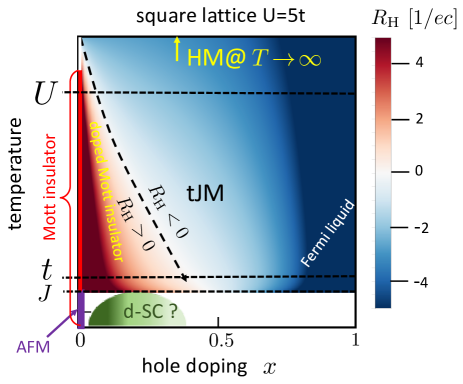
Part VII demonstrates recent application [22] of the continued fraction conductivity and Hall coefficient summation formula to strongly interacting electrons near a Mott insulator, as modelled by the two dimensional Hubbard and t-J Hamiltonians. The resulting Hall coefficient map is depicted in Fig. 1. Part VIII demonstrates the application of the same formulas to obtain the resistivity and Hall coefficient of strongly interacting lattice bosons.
Part IX summarizes the Report. A discussion of strategies for optimizing the thermodynamic approaches is given. Future applications and directions of research are proposed.
Part II Brief history of weak scattering
Perturbative calculations of Kubo formulas for DC conductivities of metals suffer from the singular effect of scattering. At leading order in impurity concentration an infinite resummation of diagrams is needed to obtain a finite longitudinal conductivity at finite impurity concentration [9].
Older (and simpler) alternatives for the weak scattering regimes are to apply the Drude and Boltzmann approaches. In this Report, unless otherwise specified, we use units of .
4 Drude theory
Drude theory [25] is particularly useful for lightly doped semiconductors. It is based on a Fermi gas of electrons of mass and charge whose kinetic energy is described by the single particle dispersion,
| (4) |
Collisions with disorder and other electrons are introduced by a scattering time . Solving for the single electron equation of motion in a time dependent field, the dynamical longitudinal conductivity is
| (5) |
where is the electron charge. The DC conductivities in a uniform magnetic field are
| (6) |
where is the cyclotron frequency, and is the speed of light. The zero field Hall coefficient is defined as,
| (7) |
Thus, is proportional to the inverse charge density. We note that , in contrast to , is independent of dynamical parameters and . Later, in Part VI, the expression of the Hall coefficient in terms of thermodynamic coefficients is shown to be a general feature of non-separable Hamiltonians.
5 Boltzmann equation
The single band Boltzmann equation (BE) [7, 8, 26] for the quasiparticle distribution function deviation is based on small deviations from the Fermi-Dirac distribution , where is the non-interacting Bloch band dispersion, is a wavevector within the Brillouin zone (BZ), and is the chemical potential. In the presence of presence of an externally imposed electrochemical field and temperature gradient , the BE is,
| (8) |
where the semiclassical equations of motion are,
| (9) |
The band and spin indices are suppressed. The band Berry curvature , which modifies the velocity [26, 27] is given by,
| (10) |
where is the periodic part of the Bloch state. is the collision integral which is commonly simplified by the relaxation time approximation,
| (11) |
Weak electron-electron and electron-phonon interactions can be incorporated into BE by renormalizing the , and contributing to the quasiparticle scattering rate .
In the absence of time-reversal symmetry breaking in the equilibrium density matrix, the electric and thermal currents are given respectively by
| (12) |
where is the Brillouin zone. Using the solution of Eq. (8) in (12), for symmetric bands, yields BE expression for the DC longitudinal and Hall conductivities,
| (13) |
For an isotropic (energy dependent) scattering time , one obtains simplified expressions at low temperatures relative to the Fermi energy ,
| (14) |
where the conductivity sum rule (CSR) is,
| (15) |
The Hall coefficient acquires a scattering time independent expression [8],
| (16) |
Eq. (16) generalizes Drude’s result (7) to non-spherical Fermi surfaces.
5.1 Example: The square lattice
The square lattice (SL) tight binding model is,
| (17) |
where creates an electron on site with spin . are nearest neighbor bonds on the square lattice (SL), and electron occupation per site is .
The Hall coefficients given by Eq. (16) and related band structure contours are depicted in Fig. 2 for nearest neighbor (nn) and next nearest neighbor (nnn) model.
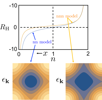
The most important prediction of Boltzmann theory is that the Hall coefficient is everywhere continuous and diverges only toward the full and empty band limits.
5.2 Conductivity relations at low temperatures
For symmetric bands, the isotropic lifetime leads to simple relations between for the longitudinal electric, thermoelectric and thermal conductivities, which can be expanded at low temperatures as
| (18) | |||||
As , one obtains the Wiedemann-Franz law
| (19) |
6 Memory Function Formalism
The Memory Function (MF) formalism [28, 29, 30] is closely related to the OHS formulation of dynamical response functions as described in Section 14.
A primary goal of the MF was to obtain the dynamical response of a set of “slow operators” which nearly commute with the Hamiltonian, by integrating out all the “fast operators” to obtain a self energy, called ‘memory matrix” . Götze-Wölfle [31] have applied the MF to evaluate the longitudinal conductivity in a weakly scattered parabolic band of effective mass ,
| (20) |
where is the current-current correlation function. They consider a white noise random potential , whose ensemble average is
| (21) |
and its commutator with the current is
| (22) |
At low temperatures, MF recovers Drude result (5),
| (23) |
The MF scattering rate agrees with Fermi’s golden rule,
| (24) |
where is the density of electron states at the Fermi energy.
More generally, the MF separation of timescales can facilitate obtaining the low temperature and frequency conductivities by renormalization of the dynamical response functions onto the low energy Hilbert space.
In Part V, the memory function can be related to the first order termination function in the continued fraction of the longitudinal conductivity.
7 Limits of weak scattering approaches
BE describes transport by quasiparticles in the conduction band, with velocity at wavevector near the Fermi surface. For elastic scattering in dimensions one and two, BE is invalidated by wavefunction localization [32, 33, 34, 35]. The collision integral of Eq. (8) describes incoherent scattering processes which do not lead to localization.
The validity of BE depends on the existence of well defined quasiparticles. Inelastic scattering broadens the quasiparticle energies and wavevectors by and . The BE therefore requires
| (25) |
The criteria (25) have been related by Ioffe and Regel (IR) [36] to experimental values of the resistivity. Using the simplified Drude theory of a parabolic band, , and , and by (5), one obtains an upper bound on value of resistivity which can be explained by Boltzmann equation,
| (26) |
For typical cubic metals with nm, the IR limit is .
In metals, usually increases with temperature due to enhanced inelastic scattering. Many metals (see review in [37]) exhibit resistivity saturation at the values not far above the IR limit.
However, resistivity in certain strongly correlated metals exceeds this limit as temperature is raised, which has been dubbed “bad metal” behavior [15]. Boltzmann equation fails to account for this regime.
In semimetals and semiconductors with a small interband gap , interband matrix elements of the current must be included when
| (27) |
This leads to a multi-band BE, which involves coupled equations for intra-band and inter-band distribution functions [38, 39, 40]. The equations are in general unwieldy. In the presence of disorder and electron-phonon scattering, a microscopic knowledge of inter-band temperature dependent scattering rates, and inter-band current matrix elements, is required.
Part III Kubo Formulas
8 Polarizations and Currents
Kubo’s formulation [16] of dynamical linear response, provides a rigorous approach to calculating conductivities of a microscopic model Hamiltonian which is supported on a finite -dimensional volume .
The underlying assumption of Kubo’s linear response theory is that local equilibrium is established throughout the sample. In other words, the currents’ equilibration length and time scales are much shorter than those of the driving fields.
Following Luttinger [18, 41, 42], it is also assumed that the same electric and thermal currents which are driven by slowly varying statistical forces, such as and , can be induced by mechanical electric and “gravitational” forces, and respectively, which couple linearly to the Hamiltonian,
| (28) |
The polarizations which couple to the external force fields are,
| (29) |
is particle density and is a local decomposition of the Hamiltonian which satisfies,
| (30) |
The Kubo formulas for conductivities require knowledge of and its polarization operators of Eq. (29). The electric and thermal currents are derived by Heisenberg’s equations,
| (31) |
We note that the polarizations (29) depend on the choice of coordinate . However, any finite shift in the origin drops out of the commutators in Eqs. (31). For PBC, uniform polarizations can be defined as a limit after taking volume to infinity, as shown later in Eqs. (69).
9 Examples: Hamiltonians and polarizations
The explicit forms of polarizations are shown for five generic models of many particle systems.
-
1.
The Hamiltonian of interacting Schrödinger particles (bosons or fermions) in first quantization notation is,
(32) where . The polarizations are given by,
(33) -
2.
Particles on a lattice with electric charge , local occupation , and hermitian two-site interaction terms:
(34) -
3.
General non-interacting (NI) normal Hamiltonians in second quantized form as
(35) where creates a particle of charge are in single-particle eigenstate with energy . denotes an anticommutator (commutator) for fermions (bosons).
The polarizations are given by the bilinear forms,
(36) -
4.
Non-interacting normal Hamiltonians of bosons or fermions with basis states per unit cell at lattice site :
(37) In a periodic crystal (PC), the Hamiltonian is given by
(38) creates a fermion (boson) state of wavevector of lattice , and basis state . After taking , the polarization operators of Eq. (36) may be represented by continuous derivatives with respect to ,
(39) -
5.
Coupled Harmonic Oscillators (CHO) Eq. can describe collective bosonic modes such as phonons [43] and magnons [44] in an insulator. A general CHO Hamiltonian which linearly couples to an external orbital magnetic field is,
(40) where denotes both site and polarization indices, where and are canonically conjugated coordinates. and are local mass and force constants. can include lattice imperfections, impurities with different masses , and boundaries. The magnetic field breaks time reversal symmetry by coupling between and as represented by a magnetization matrix . The thermal polarization is,
(41) The thermal current is obtained by Eq. (31). Using second quantized operators,
(42) the Hamiltonian is written in a duplicated Bogoliubov form,
(43) where the constant comes from the ordering the operators . The duplicated form allows us to choose to be hermitian, and to be a symmetric matrix.
can be diagonalized by a Bogoliubov transformation 111We thank Dan Arovas for sharing with us his impeccable notes defined by a symplectic matrix of size ,
(44) where , since
(45) and is a unit matrix of size . Using ,
(46) Using the relation , is determined from by the equations,
(49) (57) are readily obtained numerically by computing the right eigenvectors of the (non hermitian) matrix , and retaining those which belong to the positive spectrum . (Existence of complex eigenvalues is possible: they reflect an instability of the harmonic Hamiltonian). The upper left block yields the eigenvalue equation, for :
(58) where the eigenvectors must be normalized as,
(59)
10 Kubo formulas in Lehmann Representation
Henceforth we use unified notations
| (61) |
In the Lehmann (eigenstate) representation, the currents’ response functions are given by the sums,
| (62) | |||||
where and are the eigenenergies and eigenstates of , with as Boltzmann’s weights. are the Cartesian components of the currents.
The complex uniform () dynamical conductivities which correspond to the transport equations (1), are calculable by the Kubo formulas,
| (63) | |||||
Straightforward computation of Eqs. (62) for general many-body Hamiltonians is generally a daunting task. Exact diagonalizations (ED) of may increase exponentially with even for a single eigenstate and eigenenergy. The difficulty is compounded by the apparent necessity to compute many current matrix elements.
10.1 Non-interacting conductivities
ED is of course more manageable for non-interacting bosons and fermions. For the single particle Hamiltonian (35) and polarizations Eq. (36), using Eq. (31), the current matrix elements are,
| (64) |
The Kubo formulas reduce to sums over single particle eigenstates,
| (65) |
where
| (66) |
for fermions (bosons) with a plus (minus) sign.
11 The Tricky DC limit
DC transport coefficients require taking the orders of limits carefully. Since for any time independent Hamiltonian on a finite volume () the density matrix is in equilibrium. By definition, it cannot support any dissipative (entropy generating) steady-state transport currents. As argued by Luttinger [41], the DC steady state (which he called “rapid case”) can be achieved if the driving force satisfies , as both are taken to zero, after we have taken to eliminate finite size gaps in the continuous thermodynamic spectrum.
For thermal transport, the statistical field is replaced by Luttinger’s frequency dependent “gravitational” field [41]. The legality of this substitution has been widely accepted [18, 42], although its rigorous conditions are still debated 222Challenges to the equality of the current response to “mechanical forces” and “statistical forces” have been made by e.g. Ref [45].
In taking the DC limit, one must contend with the (superfluous) effects of the static gravitational field . This force field may create an equilibrium circulating “magnetization current” in any finite system, which is not part of the transport current [18]. It contributes to part of the Kubo formula which must be subtracted out before taking the DC limit.
In summary, the proper DC order of limits is given by
| (67) |
The causal decay of the real-time response function ensures that is analytic in the upper half plane (). Therefore the limit can be taken by a-priori setting , and sending after sending .
On finite volume, we can distinguish between OBC and PBC. For OBC, the uniform limit can be taken continuously, since the driving field is not required to be periodic between the boundaries. The DC limit is then simplified further to,
| (68) |
where the uniform polarizations are given by Eqs. (29) by setting on any finite volume. In practice, as demonstrated in in Part IV, Eq. (68) can be implemented by computing on an increasing sequence of volumes , by choosing the to be larger than the finite-size eigenenergy gaps in the Kubo formula.
On finite PBC lattices, the force fields must be continuous, and therefore their wavevectors are discretized. Therefore, in contrast to OBC, the order of limits on PBC must be taken by Eq. (67). Furthermore, since the uniform polarization cannot be taken continuously on , the limit is taken after , i.e.
| (69) |
An alternative to using the uniform polarization, the uniform electric current on a finite volume PBC can be defined as the derivative of the free energy with respect to an enclosed Aharonov-Bohm flux, see Eq. (81). No such definition exits for the thermal current.
12 Onsager relations
Under time reversal (TR) symmetry, the following operators get transformed as,
In the Kubo formulas, the order of operators gets transposed under time reversal, and the complex frequency gets transformed as
| (71) |
We note that the imaginary frequency (which describes dissipation) keeps its sign, since the entropic arrow of time remains in the future direction. If time reversal symmetry is not spontaneously broken, (i.e. there is no spin or orbital magnetization at zero magnetic field), Onsager’s relations yield,
| (72) |
For , and the longitudinal conductivities in the DC limit are symmetric in ,
| (73) |
wherev is a rotation about the axis. Thus the longitudinal conductivities are even in magnetic field at low fields. For the transverse conductivities we write,
| (74) |
where the antisymmetric part is usually called the Hall conductivity.
By Onsager relations (72),
| (75) |
For general crystal structures, , and has no special symmetry under . For the case of symmetry about , . which implies that the symmetric transverse conductivities vanish,
| (76) |
In addition, by Onsager relations and symmetry the two transverse thermoelectric coefficients in Eq. (1) coincide,
| (77) |
Eqs. (75), (77), facilitate four-probe Hall coefficient measurements by antisymmetrizing the transverse voltage with respect to magnetic field.
13 Hall conductivity proxies
For general Hamiltonians, the Kubo formula (62) for the DC Hall conductivity is computationally challenging. Hence, two simpler proxy formulas for have been very popular: (i) The Chern conductivity and (ii) the Streda conductivity . We emphasize that these proxies are only valid under restricted conditions, since they reverse the DC order of limits prescribed by Eq. (67).
13.1 Chern number
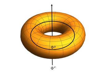
One considers a Hamiltonian
| (78) |
which describes particles with charge placed on the surface of a torus of area , with PBC. A uniform magnetic field penetrates the surface, and two Aharonov-Bohm fluxes are threaded through the and holes of the torus, as depicted in Fig. 3. The fluxes are parametrized by,
| (79) |
where is the flux quantum.
The Chern number of the ground state defined by an integral over the Berry curvature with respect to the angles :
| (80) | |||||
The Chern number is a topological integer which characterizes a gapped Quantum Hall ground state .
First order perturbation of the ground state w.r.t. the interaction
| (81) |
yields,
| (82) |
Thus the Chern number can be related to the finite volume, zero frequency Kubo formula for as given by the real part of Eq. (62):
| (83) | |||||
Thus,
| (84) |
In other words, the flux-averaged Kubo formula yields an integer times . The variation of the integrand , with flux parameters is expected to vanish in the large volume limit. The double integral can be replaced by at .
Historically, the topological relation between and the Chern number was initially discovered by Thouless, Kohmoto, Nightingale, and den Nijs, (TKNN) [12], for filled bands of non interacting, disorder-free electrons on a torus, penetrated by a unit-cell-commensurate magnetic field.
The Chern proxy for interacting Hamiltonians was derived by adiabatic transport theory by Avron and Seiler [13].
However, we must caution that reverses the proper DC order of limits prescribed by Eq. (67). Therefore the validity of this proxy is limited to the following conditions:
-
1.
For the adiabatic theorem to apply [13], a finite gap between the ground state and all excitations must exist in the infinite volume limit.
-
2.
The longitudinal conductivity must vanish . This can be ensured only at zero temperature if there are no gapless current carrying excitations and no inelastic scattering processes.
-
3.
If disorder is present it should be weak enough to prevent gapless current-carrying states from percolating through the bulk of the sample.
That said, we emphasize that has been instrumental in mathematical and experimental characterization of Quantum Hall and topological insulator phases [11, 46].
13.2 Streda formula
The Streda formula proxy for is obtained by reversing the DC order of limits of Eq. 67. In Ref. [47] it is shown that,
| (85) | |||||
where is the -magnetization and is the charge density. The last equation follows from a Maxwell relation. The Streda formula is often used to characterize quantum Hall phases and topological insulators by scanning compressibility measurements [48].
In general the Streda order of limits does not commute with the DC order of limits (67), and therefore
| (86) |
The conditions which may permit the use Streda’s proxy is that the ground state is bulk-incompressible, and that the Hall angle is large, i.e. . Such conditions occur when there is a gap for excitations above the ground state, and the temperature is lower than this gap. A weaker condition is a pseudogap, where the density of charge excitations vanishes rapidly enough at low energies to allow reversal of the order of limits in the Kubo formula.
14 Kubo formulas in operator Hilbert space
The Kubo formulas of Eq. (62) may be formulated as matrix elements in OHS. This formalism avoids the Lehmann representation, and proves to be convenient for further mathematical manipulation. Below, we shall use the OHS formalism to derive the DPP formulas in Part IV, the continued fractions in Section 21, and the Hall coefficient summation formulas in Part VI. We start with the formulation of susceptibilities as inner product in OHS. We then proceed to formulate dynamical response functions in OHS.
14.1 Equilibrium Susceptibilities
Given a static Hamiltonian and free energy,
| (87) |
A thermodynamic expectation value is given by,
| (88) | |||||
where Boltzmann weights are . Static susceptibilities with respect to and are,
| (89) | |||||
where . In the second line . The last line of (89) is written in the Lehmann representation of . The vector space of linear operators which act within the Schroedinger Hilbert space of the Hamiltonian , is an OHS containing hyperstates , and closed under linear superpositions. Henceforth we consider general operators , whose susceptibility is
| (90) |
defines the Bogoliubov-Mori (BM) inner product, [28] which depends on (with its boundary conditions) and inverse temperature . It obeys the Hilbert space conditions of (i) a positive norm, (ii) hermiticity and (iii) linearity,
| (91) |
All operators which commute with are identified with the null hyperstate of zero norm.
14.2 The Liouvillian and its inverse
In OHS, the Liouvillian hyperoperator , which generates the time evolution of hyperstates, is defined by,
| (92) |
where is any operator in the Hilbert space of .
Lemma 1.
The Liouvillian is a hermitian hyperoperator in OHS,
Proof.
| (93) | |||||
where the summation indices are relabelled in the last equation. ∎
is therefore diagonalizable. Its eigenoperators are with real eigenvalues . It is the generator of time evolution in the OHS, since
| (94) |
The inverse Liouvillian does not exist if the kernel of is non zero. Hence we define it with an imaginary infinitesimal prescription,
| (95) |
where the real part of the inverse is the hyperoperator
| (96) |
and the imaginary part is
| (97) |
The weight of the inner product, Eq. (90) can be expressed as
| (98) |
Using Eq. (96) we can write BM inner product in a representation independent form,
| (99) | |||||
The advantage of Eq. (99) over Eq. (90) will be made clear during the mathematical manipulations of the Kubo formulas performed in the following Sections.
14.3 Dynamical linear response functions
Dynamical response functions are obtained in linear response by adding to the Hamiltonian a weak time-dependent field coupled to an operator . The field is turned at ,
| (100) |
At the expectation value of an observable is
| (101) |
where the density matrix and the evolution operator satisfies . Expanding to linear order in yields,
| (102) |
where , and using to obtain . The transform of (102) into the upper complex plane defines the complex response function,
| (103) | |||||
14.4 Electric and Thermal conductivities
Part IV DPP Hall conductivities
15 Derivation of DPP formulas
For simplicity the magnetic field is chosen along the axis and symmetry is assumed in the plane. According to Eq. (67), the DC Hall-type conductivities are given by,
| (105) |
As mentioned before, the second term cancels the spurious magnetization currents which are created by the static component of the “gravitational” field . In OHS notation,
| (106) |
where -dependence of the currents is implicit. Under rotation in the plane , and since the second term is symmetric under , it vanishes. In the Lehmann representation,
| (107) |
At first glance, one might be tempted to discard contributions in the denominator of Eq. (107). On OBC, this would be a gross error! As shown below, the DC limit is dominated by eigenstates with .
Using the identity (99),
| (108) |
To remain consistent with symmetry, on finite volumes we identify , while keeping the DC order of limits in Eq. (105). By Eq. (31),
| (109) |
is a Lorentzian degeneracy projector,
| (110) |
and are DPP’s (degeneracy projected polarizations), whose matrix elements in the Lehmann representation are restricted (at small ) to connect quasi-degenerate eigenstates,
| (111) |
Eq. (108) can be written as
| (112) |
Expansion of the terms in (112) we obtain a sum of four terms,
| (113) |
The first term, which is independent of and is called a magnetization term,
| (114) |
The physical content of magnetization terms is discussed in Section 15.1. The magnetization term precisely cancels the second term in Eq. (105), and therefore does not need to be calculated for the Hall-type conductivity.
The remaining three terms are related to each other,
| (115) |
and contain one DPP, and therefore a Lorentzian factor, . contains a Lorentzian square . The Lorentzian factor and its square can be effectively replaced for small by box projectors and , respectively. Since we are taking , (after ), the three terms have the same DC limit,
| (116) |
Thus, summing up Eq. (113) the DC Hall conductivities are given by the DPP formulas,
| (117) |
Here we have restored the dimensionful dependence on and for practical applications.
15.1 The Magnetization terms
The terms in Eq. (114) cancel against their counterterms in Eq. (105). For electric Hall conductivity , the magnetization term vanishes since the two polarizations commute: . The thermoelectric and thermal Hall magnetization terms do not vanish. For Schrödinger particles governed by , the polarization commutators can be readily calculated to yield,
| (118) |
which agrees with Ref. [18, 19]. and are the -direction electric and thermal magnetization densities respectively.
The magnetization subtractions create considerable headache when computing the Kubo formulas from Eq. (62). Since are weighted by in Eqs. (63), any separate approximations of the two terms in Eq. (105) could result in an error which embarassingly diverges at low temperature. (Heat conductivities should actually vanish at low temperatures by the third law of thermodynamics). Elimination of these subtractions from the DPP formulas (117) provides an essential simplification.
16 DPP formulas for non-interacting Hamiltonians
For a normal Hamiltonian of non-interacting fermions or bosons, Eq. (35), the DPP formula is
| (119) | |||||
where the polarizations are defined in (36), and their DPP’s are given by
| (120) |
At low temperatures, the factor ensures the sum is dominated by excitation energies at less than of order from the chemical potential.
For a bosonic Hamiltonian of coupled harmonic oscillators (40), the thermal polarization is generally an anomalous bilinear form given by Eq. (60). The anomalous matrix blocks involve creation or annihilation of two positive energy states, such that . Thus, there are no anomalous contributions to the DPP 333Unlike their conttribution to the magnetization terms. It is good to know that anomalius terms are projected out, since their commutator would lead to diverging contributions to the low temperature limit of .. Thus we are left with the normal parts of the polarizations,
| (121) |
17 Berry curvature integrals
Hall-type conductivities for non-interacting periodic crystal Hamiltonians , defined in Eq. (38), can be expressed as Berry curvature integrals over BZ, where the band Berry curvature is defined in Eq. (10).
The relations between Berry curvature integrals and Hall conductivity [27], Transverse thermoelectric conductivity [49] and thermal Hallconductivity [19, 50], have been previously derived from semiclassical dynamics and also directly from the Kubo formula of perfectly periodic lattices (65).
Here we provide a somewhat simpler derivation (in our view) starting from the single-particle DPP formulas for periodic lattices. is a unitary matrix which diagonalizes in , and defines the eigenmode operators,
| (122) |
such that,
| (123) |
The uniform polarizations can be defined by sending after in Eq. (39), (see Eq. (69):
| (124) |
The DPP operators are constrained to act only within the same band . Using Eq. (122), the electric DPP’s are given by
| (125) |
The vector function is the Berry gauge field [51] of eigenmode ,
| (126) |
Similarly, the thermal DPP’s are
| (127) |
where . Note that on a finite volume, are discrete with intervals of . The DC limit is obtained by keeping , as . The differentiability of and allows us to set in Eqs. (125) and (127), which involve a relative correction of .
By (125) the commutator
| (128) | |||||
where we discarded when acting on differentiable wavefunctions. defines the Berry curvature field in the direction of eigenmode .
By Eq. (117) the intrinsic Hall conductivity recovers the result of Chang and Niu [27],
| (129) |
This expression has been used to describe the anomalous Hall effect in ferromagnets [52]. Additional effects of impurities have been introduced semiclassically [53].
The thermal Hall DPP’s have a slightly more complicated commutator,
| (130) | |||||
where .
For convenience we define energy resolved conductivities by,
| (131) |
In three dimensions, for fixed , the function restricts the wavevectors to a circle on sphere of energy , such that
| (132) |
Thus, we use Stokes theorem to relate to by,
| (133) | |||||
Thus, we arrive at the expression previously derived by Qin, Niu and Shi [19],
| (134) | |||||
Similarly, the DPP formula for the thermoelectric conductivity of a clean -symmetric metallic band of electrons with charge , is given by
| (135) |
Using (128) and defining,
| (136) |
one can express,
| (137) |
For low temperatures Eqs. (134) and (137) for metals reduce to the relations,
| (138) |
these relations extend Mott relations [54] between electric and thermoelectric conductivities to bandstructures with Berry curvatures [49].
Introducing the effects of disorder in the anomalous Hall effect has been a major challenge in the field. The main difficulty is to extend the semiclassical analysis to include effects of short range scattering [53, 55, 56, 57]. The general non-interacting DPP formulas (119) can feasibly study effects of disorder numerically.
18 DPP formula for confined Landau levels
We consider an electron in a uniform magnetic field , with vector potential , In first quantized notation, the Landau operators are,
| (139) |
The Landau level (LL) raising and lowering operators are respectively,
| (140) |
where , and the Landau length is .
The LL Hamiltonian is
| (141) |
where the cyclotron frequency is . The eigenenergies are
| (142) |
where the integer LL index is , and is the number of states per area in each LL.
The guiding center operators are,
| (143) |
where
| (144) |
The polarization operators are
| (145) |
Since change the LL index by , while connect states within each LL. Hence under degeneracy projection, the -operators are projected out, and DPP’s are simply proportional to the guiding center operators,
| (146) |
The DPP Hall conductivity formula (119) yields
| (147) | |||||
where is the electron density.
While the sum in Eq. (147) includes all occupied states, Eq. (119) shows that the Hall conductivity can be written only in terms of states near the Fermi energy .
Where are these current carrying states? On finite systems with OBC, the semiclassical eigenenergies in each LL (which apply for smooth confining potential on the scale of ), reach the Fermi energy at the sample edges. Each LL band contributes one gapless edge mode. The Hall conductivity is precisely given by Eq. (147).
19 DPP Hall conductivity in a disordered metal
In the weak disorder and magnetic field regime proxies such as Chern numbers and Streda formulas do not work, since disorder mixes Landau levels, and the longitudinal conductivity is finite. Since strongly depends on the scattering lifetime, it is instructive to compare Boltzmann’s theory to the Kubo formula by numerically calculating it via the DPP formalism. It also gives us a chance to demonstrate how the DC limit is taken in a metallic gapless system.
In Ref. [58], the weakly disordered square lattice (DSL) Hamiltonian was considered,
| (148) |
where is a uniformly distributed random number and is the magnetic fux per plaquette. Using the DPP formula (117), we compute the disordered averaged curves for a sequence of linear sizes , as shown in Fig. 4.
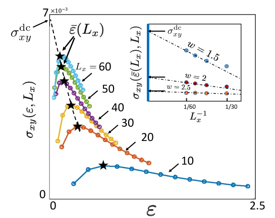
For each curve we determine by
| (149) |
which is marked by black star in Fig. 4. These values fit the function . This scaling is consistent with level spacings of one dimensional extended states.
The DC conductivity is estimated by graphically extrapolating the sequence,
| (150) |
In the inset of Figure 4, we extrapolate the Hall conductivities at various values of disorder strength to their their respective DC limits.
20 Physical consequences of DPP formulas
The first implication of Eqs. (117) is that the Hall conductivities are on-shell expressions which is in apparent contrast to the original Kubo formula (107). Furthermore, at low temperatures, the conductivity is dominated by the low energy excitations . Conceptual conclusions from the DPP formulas are:
-
1.
A OBC system exhibiting a non-zero Hall-type conductivity possesses a quasi-degenerate (gapless) manifolds of eigenstates which are created by the presence of the magnetic field.
-
2.
At low temperatures, since the DPP’s involve low energy eigenstates, it is easy to see that and vanish as . It is also simple to verify for phonons and spin-wave models, that the anomalous (i.e. ) terms in the current operators.
-
3.
These manifolds are subjected to the non commutative geometry generated by the DPP’s. That is to say, since
(151) then acts as a conjugate momentum to . The DPP’s are therefore similar in spirit to the non-commuting guiding center coordinates which act within a quasi-degerenate Landau level in the strong magnetic field limit.
-
4.
In quantum Hall and topological insulator phases, the Hall-current carrying states are be supported on the OBC sample edges. For compressible metallic phases, the Hall current is carried on chiral extended states which percolate through the bulk. An explicit description of these states has been used by Chalker and Coddington model [59] to describe the quantum-percolation transition between Hall plateaux.
- 5.
Numerical advantages.– The elimination of the higher eigenstates in the DPP formulas at low temperatures allows us to replace by its effective Hamiltonian renormalized onto the lower energy Hilbert space. may be computationally easier to work with than .
Part V Continued fractions of longitudinal conductivities
21 Moments expansion
Real longitudinal conductivities (in the direction) are given by the real part of Eq. (104),
| (152) |
where is a broadened Dirac -function of width . Henceforth we suppress dependence, keeping in mind the eventual correct DC order of limits of Eq. (67). For the moments expansion we define a symmetrized mixed electric+thermal current as
| (153) |
Thus, the thermoelectric conductivity can be written as a sum of auto-correlation functions,
| (154) |
Henceforth we discuss and suppress the currents’ label .
The moment of order of is
| (155) | |||||
The moment is the CSR,
| (156) |
All odd moments vanish by antisymmetry of ,
| (157) |
Moments are thermodynamic expectation values of time-independent operators,
| (158) | |||||
where we used Eq. (99) and is the -polarization corresponding to by Eq. (31).
Moments are coefficients of the short time Taylor series of the real-time conductivity,
| (159) | |||||
Unfortunately, a finite set of moments cannot, in general, determine the long time behavior of Eq. (159), and the low frequency behavior of Eq. (152).
The following constraints can be very helpful in guiding us to a viable extrapolation scheme to high orders.
-
1.
Since is a non-negative Hermitian hyperoperator, is a non-negative spectral function.
-
2.
, which therefore permits a finite DC conductivity at .
-
3.
All the moments are squares of norms , and therefore non negative.
-
4.
By thermodynamic arguments, the real-time conductivities of Eq. (159) should be continuous and differentiable for . Also, they are expected to decay (relax) at long times. This ensures the analyticity of in the upper half plane . 444The only notable exception is in a superconductor, where persistent currents do not decay. For superconductors, the zero frequency conductivity is excluded from . Thus, by (159), the asymptotic growth of the high order moments is bounded by,
(160)
21.1 Krylov bases
An orthonormal Krylov basis of hyperstates can be constructed from the current operator. We start with the normalized root (zeroth order) state,
| (161) |
( denotes normalized hyperstates, in contrast to non normalized hyperstates such as .)
Higher order Krylov hyperstates are inductively generated by the equations
| (162) |
where is the recurrent of order , which is equal to the matrix elements of the Liouvillian,
| (163) |
In order to evaluate the following statements are verified:
-
1.
The Liouvillian expectation values vanish in the Krylov basis. By construction of Eq. (162), even (odd) order Krylov hyperstates involve states with even (odd) powers . Hence we can expand any Krylov hyperstate as
(164) The expectation values of in Krylov hyperstates are,
(165) which follows from Eq. (157).
- 2.
-
3.
The Liouvillian representation in the Krylov basis is,
(174) The matrix can be regarded as a tight binding hopping Hamiltonian on a half chain, with hopping parameters .
-
4.
The phases of can be chosen such that we can gauge all the recurrents to be real and positive.
is the “Liouvillian Green function”,
| (175) |
Since is symmetric, so is , which is in general complex. On the real axis , is a spectral function. It is non-negative and symmetric in . The real part of the complex function can be obtained from the spectral function by the Kramers-Kronig (KK) transform,
| (176) |
, and by Eq. (176), . Non diagonal Green functions can be obtained from the inversion equation ,
| (177) |
For example,
| (178) |
and generally,
| (179) |
Another important relation is,
| (180) |
which is purely real. As a consequence, the matrix elements of the imaginary inverse Liouvillian do not connect to the first Krylov state:
| (181) |
This result will prove to be useful in Section 24.
21.2 The continued fraction representation
Since is a tridiagonal matrix, an iterative inversion can be used to invert in Eq. (175), and express it as
where is the termination Green function on the half-chain with the sites . The sequence of equations (LABEL:CF1) comprises an infinite continued fraction (CF),
| (183) |
22 From moments to recurrents
The first question that comes to mind is: How do we obtain the recurrents , from a given sequence of moments ?
Eq. (155) and (174) generate a sequence of identities:
| (184) |
Importantly, depend only on the recurrents . This allows us to solve for the recurrents iteratively, starting at . As a result we obtain the algebraic equations,
| (185) |
In general increase very rapidly (of order ) with , while are much smaller numbers which increase at a much slower rate. The presence of subtractions in Eq. (185) imply that small relative errors in may result in large relative errors in 555We thank Snir Gazit for alerting us to this numerical challenge.
22.1 Single Mode Spectra
Let us start with a single sharp mode at zero frequency as shown in Fig. 6(a),
| (186) |
All the recurrents vanish identically, since .
| (187) |
A single mode at finite frequency is shown in Fig. 6(b). It is described by
| (188) |
The only non-zero recurrent is . Physically this occurs when is an eigen-operator of the Liouvillian
| (189) |
and therefore applying to the Hamiltonian’s ground state creates an eigenstate with excitation energy .
An approximation which assumes a spectral function which approximately is described by a -function, is the single mode approximation. This approximation was used by Feynman [63] to describe the roton minima in the spectrum of superfluid helium [63], by Girvin, Macdonald and Platzman [64] to describe the magneto-roton excitation of the Fractional Quantum Hall phase, in Refs. [65, 66] to approximate the Haldane gap in a spin-one chain model.
23 From recurrents to conductivities
The longitudinal conductivity of Eq. (152) is determined by the zeroth order spectral function,
| (190) | |||||
where is the infinite tridiagonal matrix of Eq. (174), and is defined as a CF in Eq. (183).
In practice, the calculation of is limited to a finite sequence. However, truncating the CF at any finite order does not lead to a continuous function, but to a sequence of -functions. In effect, determining amounts to inversion of the moments series, which is in general and unsolved problem.
CF however allow us to design extrapolation schemes which may be suitable for certain class of physical problems, which provide additional information about the desired . For example, is a positive and symmetric function, whose all its recurrents are finite, non-negative numbers.
Since extrapolation is a tricky art, it is useful to first learn about rigorous results relating high frequency asymptotics of and high order recurrents.
23.1 Freud’s high order asymptotics
For a large class of smooth spectral function with support on the whole frequency axis 666We thank Ari Turner for explaining to us the mathematical literature reviewed in this section, Freud [67] has conjectured an asymptotic relation between the high frequency asymptotic fall-off of the spectral function, and the asymptotic behavior of the high order recurrents as .
This conjecture was proven by Lubinsky, Mhaskar and Saff (LMS) [68], for spectral functions described by
| (191) |
The fall-off exponent is assumed to satisfy the following conditions:
-
1.
.
-
2.
exists for , and is bounded near the origin as . Furthermore, exists for large enough .
-
3.
For finite values of at large enough ,
(192)
LMS proved that the corresponding recurrents for Eq. (191) exhibit the asymptotic behavior,
| (193) |
Interestingly, for pure stretched exponential
| (194) |
as shown in Figs. 7 and 8, the exact low order recurrents are close but slightly different from the analytic asymptotic values of Eq. (193), except for the pure Gaussian , for which Eq. (193) is exact.
In general, since the moments and recurrents are non-negative, by Eqs. (184), the moments grow at least as fast as
| (195) |
Due to assumed continuity of on the real-time axis, by Eq. (160), the moments cannot grow faster than .
This implies that for continuous and bounded response functions, the asymptotic power of is limited to
| (196) |
23.2 Termination functions
Assume that we have calculated a finite set of recurrents
| (197) |
This finite set is not sufficient to describe the continuous function . Extrapolation of recurrents is tantamount to finding an accurate termination function such that,
| (198) |
is the normalized CF which contains only the higher order recurrents ,
| (199) |
If are the known recurrents of a complex variational spectral function . The variational reurrents are used to produce the termination function by iteratively inverting the CF of the complex function ,
| (200) |
We emphasize that or the inversion, both real and imaginary parts of are required, where the real part is obtained by a Kramers-Kronig transformation, Eq. (176), of the imaginary part.
Termination functions can be used to study the effects of low order recurrents on the frequency dependence of .
23.3 Low frequency behavior
By LMS theorem, the high order recurrents can determine high frequency decay of a large class of spectral functions. Conversely, low frequency behavior can be deduced in certain cases from the low order recurrents. We first demonstrate the low frequency effects of varying the first recurrent, and then we show the low frequency effects of alternating even-odd deviations of recurrents from their high order asymptotic behavior.
The recurrents of the semicircle spectral function function,
| (201) |
are,
| (202) |
The recurrents of a Gaussian spectral function are,
| (203) |
are,
| (204) |
As noted by the memory function approach, in the weak scattering limit, the first order recurrent plays an important role in determining the low frequency conductivity.
The first recurrent dominates the DC conductivity. This is demonstrated by varying in Fig. 9, keeping the higher order recurrents the same. For both the Gaussian in Fig. 9, and the semicircle in Fig. 10, the DC limit of the resulting normalized modified functions vary with as
| (205) |
Stronger modifications of the low frequency behavior is produced by even-odd deviations of the recurrents from the asymptotic form. This is demonstrated by the power-law times Gaussian function (PG), as discussed in detail in Ref. [21],
| (206) |
The recurrents of the PG have been evaluated analytically,
| (207) |
and are plotted versus their low order recurrents in Fig. (11). The zero frequency conductivity vanishes or diverges depending on the sign of . While the relative deviations from the asymptotic behavior at large decreases, the effects of the low order recurrents are dramatic at low frequencies. A similar effect is seen numerically for power law functions times stretched exponentials at [21].
23.4 Addition of spectral functions with different frequency scales
The low frequency regime of the response function affects the behavior of the recurrents in a more complicated way than the high frequency asymptotics. For example we consider a sum of two semicircles with different energy scales
| (208) |
where is given by Eq. (201). may be positive (for enhanced DC conductivity), or negative, for suppressed DC conductivity. The moments are additive,
| (209) |
(where we must use , since all moments must be non-negative). After hashing the algebraic relations (185), the combined recurrents are highly entangled. The effects of summing two spectral functions are shown in Fig. 12. The addition of two spectral functions results in even-odd oscillations of the recurrents which persist to high orders, although its signature is already observed at low orders.
23.5 Variational Extrapolation of Recurrents
Since nested commutators of the Hamiltonian with the current create a factorial growth of number of operators, the computational cost of high order moments and recurrents in many cases increases faster than exponentially.
Here we describe the Variational Extrapolation of Recurrents as a possible scheme which allows for a numerical test of its convergence.
Having computed , may lead to a reasonable guess for the possible asymptotic behavior at large and low frequencies. We choose a family of analytic variational spectral functions , which can be parametrized by variational parameters .
Using Kramers-Kronig relation (176) find the real part of ,
| (210) |
and calculate the variational recurrents from the lowest moments of .
The variational parameters are obtained by minimizing the least squares function with respect to ,
| (211) |
The lower cut-off is chosen to preferentially fit the recurrents of to the higher orders of the calculated recurrents. The total number of variational parameters must be smaller than to avoid overfitting.
Inverting Eq. (198) provides which directly provides the Variational Extrapolation of Recurrents (VER) approximation for ,
| (212) |
The spectral function is given by,
| (213) |
Eq. (213) shows that the imaginary part of is due to the complex termination function with . The quality of the VER can be tested by two criteria: (i) The in (211) should be much less than unity. (ii) Computing some additional recurrents and comparing them to the extrapolated .
Part VI Hall coefficients summation formulas
For simplicity, the magnetic field is chosen along the axis and symmetry is assumed in the plane. The Hall-type coefficients are the electric Hall coefficient , the Nernst Coefficient , and the thermal Hall coefficient :
The coefficients in Eq. (VI) exist if we assume that
| (214) |
That is to say, the expressions apply to gapless dissipative phases, and do not apply to superconductor, insulator, or quantum Hall phases. In addition we also assume no spontaneous magnetization at zero magnetic field, which implies no anomalous Hall effect.
Straightforward Kubo formula calculations of Eq. (VI) demand determination of both longitudinal and Hall conductivities. The summation formulas [47, 69] derived below, replaces the difficulties of DC Kubo formulas by calculations of thermodynamic coefficients.
24 Magnetic Field Expansion of Hall-type Conductivity
The derivative with respect to the magnetic field is very difficult to perform using the Lehmann representation, which requires taking derivatives of current operators, wavefunctions, and eigenenergies.
It is therefore much more convenient to differentiate by parts the DC Hall conductivities as written in Eq. (112),
| (215) | |||||
We assume OBC in order to define uniform polarizations. OBC are also required to continuously vary the magnetic field and avoid Dirac’s quantization [70].
vanishes under the trace by even time reversal symmetry of at , and odd symmetry of :
| (216) | |||||
The remaining term is calculated by differentiating the hyper-projector (110) with respect to ,
| (217) | |||||
The hypermagnetization is defined by
| (218) |
where . 777Note: Under TR, , and the commutators in the response functions reverse their order . Therefore the hypermagnetization is even under TR.
Thus we obtain,
| (219) | |||||
In the last row of (219), we applied Eq. (99) to reconstruct the OHS current matrix element. The vanishing of is proven as follows. Using the hermiticity of (93), we can write:
| (220) | |||||
Next, we will prove that,
| (221) |
The inner product of the hyperstate given by Eq. (221) with any Krylov basis hyperstate belonging to the same root current is,
| (222) | |||||
since is purely real, as proven in Eq. (181).
In contrast to Eq. (221), the surviving terms in (219) do not vanish since,
| (223) | |||||
where the last identity uses Eq. (179).
Thus we obtain
| (224) |
It is possible to evaluate Eq. (224) by inserting two Krylov bases resolutions of identity,
| (225) |
where is the projector onto OHS subspace spanned by the hyperstates for . Using the symmetry, we obtain
| (226) | |||||
where are the -hypermagnetization normalized matrix elements between Krylov hyperstates,
| (227) |
By Eq. (179),
| (228) |
and by Eq. (63),
| (229) |
Thus the sum over in Eq. (226) includes only even integers and results in the summation formula,
| (230) |
The longitudinal conductivities and factor out of the sum in Eq. (230). They produce the non-commuting DC limit of .
25 Hall Coefficient
In the double summation over the Krylov bases we separate out the term write the electric Hall coefficient as a sum of two terms,
| (231) |
where
| (232) |
is the zeroth moment of the longitudinal conductivity, which was defined in Section 21. It represents the kinetic energy of the constituent charge carriers. The current-magnetization-current (CMC) susceptibility, , measures the effect of the Lorentz force on the currents, as shown below. reproduces Boltzmann’s equation result for energy dependent scattering time [71].
The correction term involves higher order recurrents and hypermagnetization matrix elements, defined in (226). The recurrents and Krylov operators involve current non-conservation, caused by disorder, hard core interactions and lattice Umklapp scattering. These terms are increasingly difficult to compute. In order to be allowed to neglect them, they must be estimated to be smaller in magnitude than . In Section 31 and Section 34, such estimates are obtained by calculation of the lowest order terms for certain lattice models of strongly interacting electrons and hard core bosons.
The current-magnetization-current (CMC) susceptibility, , measures the effect of the Lorentz force on the currents, as shown below. reproduces Boltzmann’s equation result for energy dependent scattering time [71]. includes the higher order corrections due to disorder, hard core interactions and lattice Umklapp scattering. For Hard Core Bosons, will be partially evaluated in subsection 34.4.
25.1 Weak scattering limit
26 Modified Nernst Coefficient
The Modified Nernst Coefficient for symmetric Hamiltonians is
| (234) |
can be expressed by the summation formula,
| (235) |
where
| (236) |
and are the thermal CSR, and thermoelectric hypermagnetization matrix elements respectively. is therefore expressed as a thermodynamic coefficient similar to , and which follows below.
27 Thermal Hall coefficient
The thermal Hall coefficient is,
| (237) |
where
| (238) |
28 Calculating the correction terms
The correction terms in Eqs. (232,236,238) depend on recurrents , which demand calculations of moments , and hypermagnetization matrix elements . The latter are most conveniently derived from the non-normalized magnetization matrix elements
| (239) |
which are thermodynamic expectation values of nested commutators. For short range Hamiltonians, the commutators include sums over connected clusters of operators which are easier to trace over than calculating two-operator susceptibilities. These clusters can be generated and traced over by symbolic manipulation, as demonstrated in Sections 31 and 34.
are related to of the correction terms by the Gramm-Schmidt matrix . This matrix is determined as follows. Applying the resolution of identity with the Krylov basis,
| (240) | |||||
The matrix is obtained by powers of the tridiagonal Liouvillian matrix (174), which results in polynomials of the recurrents ,
| (241) |
Thus we obtain,
| (242) |
29 Optimization of thermodynamic approaches
29.1 The Separability problem
The thermodynamic approaches have their limitations. The continued fraction extrapolation can only be performed efficiently if a clear asymptotic power law can be deduced from the dependence of the calculated recurrents on their order. In practice, the fluctuations of the calculated recurrents from an asymptotic power law behavior should decrease monotonically if a reliable termination function is to be found.
Nearly separable currents can significantly slow the convergence of continued fractions and Hall coefficients corrections. For example, the recurrents of a sum of two spectral functions with very different characteristic frequency scales is shown in Fig. 12. We note that the fluctuations about average recurrents do not converge rapidly.
Physically, sums of spectral functions with vastly different frequency scales can be expected for separable currents with different relaxation times. That is to say, if the Hamiltonian and its currents can be written as sum of commuting channels,
| (243) |
the resulting conductivities will be sums,
| (244) |
While their moments are additive,
| (245) |
the recurrents which are obtained by Eqs. (185) are highly entangled functions of the separate ’s.
Similarly, the Hall coefficient summation formulas are formally correct, but cease to be useful for separable currents. Since the total Hall coefficient is,
| (246) |
for multichannel separable currents , ratios between different conductivities must enter the Hall coefficient, which therefore cannot be captured accurately just by . For example, Fermi surface electrons with strongly dependent -dependent lifetime . At weak scattering, the currents of different wavevectors are separable. While of Eq. (232) recovers the single lifetime expression of Eq. 14, it does not agree (within a factor of order unity) with the -dependent lifetime result of Boltzmann’s equation in Eq. 13. The difference between and Boltzmann’s result is contained in the higher order correction terms, which are unwieldy.
In conclusion, continued fractions and Hall coefficient summation formulas are best suited for a non-separable current governed by one relaxation timescale. Otherwise, in Hamiltonians which support two or more separable currents with different relaxation tiemscales, the conductivities of each current should be calculated separately and later assembled in Eq. (246) to obtain the total Hall coefficient.888We thank Steve Kivelson for emphasizing the anistropic lifetime problem in the Hall coefficient formula.
29.2 Renormalized Hamiltonians at low temperatures
Effective Hamiltonians are crucially important for efficient use of thermodynamic approaches to DC transport coefficients. As can be seen from the Lehmann representation of longitudinal conductivities (62), and the DPP formulas of the Hall conductivities (113), the important part of the spectrum and eigenstates resides in an energy window of order above the ground state. The Hall coefficient formula, which is derived from Eq. (224), also depends on that part of the spectrum as can be seen from,
| (247) |
where . Thus, in the DC limit, is also an on-shell expression. It is greatly advantageous to replace the microscopic Hamiltonian by an effective Hamiltonian which operates in the low energy Hilbert space and reproduces the correct spectrum at .
The renormalized currents and magnetization within this reduced Hilbert space are defined by,
| (248) |
where are also projected onto the reduced Hilbert space. A consequence of renormalization in certain models is to reduce the magnitude of currents’ non-conservation, i.e.
| (249) |
The relative magnitude of the first recurrent depends on this commutator. Since all terms in the Hall coefficient’s correction terms are proportional to , this ensures reduction of the relative magnitude .
An simple example of the value of renormalization is demonstrated by comparing the zeroth Hall coefficients of the microscopic Hamiltonian of electrons in a periodic potential, to that of the conduction band effective Hamiltonian. The microscopic Hamiltonian is goven in Eq. (32). Its magnetization is given by
| (250) |
The CSR and CMC are completely independent on the potential terms and hence,
| (251) |
Where includes the electrons in all the filled bands and core states. The zeroth Hall coefficient must clearly be very far from the full answer, since we know from Boltzmann’s equation (16) that depends only on the filling of the conduction band. The correction term is therefore expected to be significant. Indeed, the magnitude of the first recurrent , which is a factor in is of order
| (252) |
which can be very large for crystal potentials .
In comparison, if we use the renormalized conduction band Hamiltonian,
| (253) |
where is due to impurities, then
| (254) |
is just the density of the partially filled conduction band. recovers Drude-Boltzmann theory (7), with a small correction term which is suppressed by a factor of .
For dirty semimetals [71], where the interband gap is of the same order as , the Hall coefficient can be well approximated by of the two-band Hamiltonian, including both intraband and interband current matrix elements. The Hall coefficient formula provides a simpler route to the Hall coefficient than the coupled two-band Boltzmann equation [38, 39, 40].
Part VII Strongly Correlated Electrons
30 The Hubbard Model
Electrons in a tight binding bandstructure, with strong local interactions can be minimally described by the Hubbard model (HM) [72, 73], which on the SL is given by
| (255) |
For historical reasons, the electron filling in the HM is often measured by the “hole concentration” relative to half filling, i.e. , as defined by .
For the HM reduces to the non-interacting nn SL model, which was discussed in Section 5.1. As shown in subsection 25.1, reduces to Boltzmann’s equation isotropic scattering time result, which was depicted in Fig. 2.
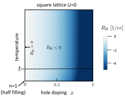
The Hall coefficient temperature-doping map of the nn SL model, is depicted in Fig. 13. We note that the Hall sign is negative for all , and vanishes half filling . This Hall map will be contrasted with the Hall map in the regime.
31 The tJ Model
In the strong interacting regime of , the electronic correlations of the HM differ drammatically from the predictions of the weakly interacting model on the SL. This is true especially near half filling , where a charge gap of order appears between the singly occupied spin and hole configurations, and configurations which contain doubly occupied sites. At zero temperature , the half filled HM describes a Mott insulator, which orders antiferromagnetically. Away from half filling, the ground state phase diagram is still under debate, with variational studies indicating possible charge and spin density wave order, and/or -wave superconducting order [5, 23, 73].
As argued in subsection 29.2, at temperatures , the thermodynamic approaches converge much better after the HM Hamiltonian is renormalized onto its lower energy Gutzwiller-projected (GP) subspace of no-double-occupancies. There, for , the HM maps onto the t-J model (tJM) [66, 74], which to second leading order in ,
| (256) |
The GP bond operators are
| (257) |
where . () describes the bond kinetic energy (current) and describes the spin-dependent hopping. is Anderson’s antiferromagnetic superexchange energy.
31.1 Linear Resistivity slope
The t model, , dominates the metallic charge transport at . The doping dependence of the CSR of the t model was calculated by Jaklic [75] and Perepelitsky [76] up to order :
| (258) |
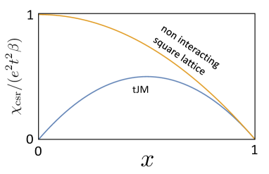
As depicted in Fig. 14, the CSR vanishes toward as a consequence of the GP. It is also suppressed relative to the non-interacting limit even far from half filling. Vanishing of the CSR produces a divergence of the Hall coefficient by Eq. (305).
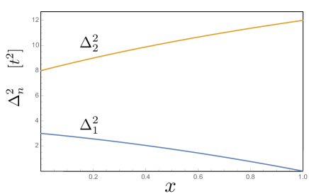
The high temperature limit of the first two conductivity recurrents of are,
| (259) |
which yields the CF of the DC conductivity as,
| (260) |
Due to lack of higher order recurrents, is approximated by extrapolating the recurrents using semicircle termination (sct) (see Eq. (202)), and Gaussian termination (gt) (see Eq. (204)),
| (261) |
In Fig. 16, the high temperature DC resistivity slopes of are plotted for both termination approximtions. We see that the slopes diverge toward the Mott limit, as expected by the suppression of the CSR depicted in Fig. 14. Interestingly, the resistivity is finite at high temperatures even in the dilute electron density limit . The slopes of Fig. 16 are in qualitative agreement with the HM calculation in Ref. [77].
31.2 Hall map for large
of the t-model was calculated by Eq. (232). The doping dependent CMC was determined up to order ,
| (262) | |||||
The zeroth Hall coefficient was determined up to second order in ,
| (263) |
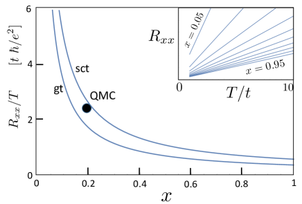
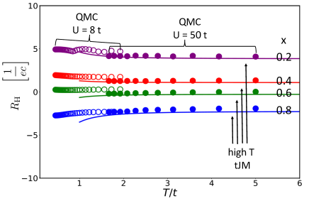
The calculation of was extended down to the intermediate temperature (IT) regime: , by Quantum Monte Carlo (QMC) simulation, using the full HM weights at large . The QMC calculation includes the effects of the spin interactions in the tJM. The QMC data is plotted in Fig. 17, with the analytic curves of Eq. (263) which are depicted by solid lines.
At extremely high temperatures , one must use the unprojected HM of Eq. (255). The suppression of double occupancies in the HM diminishes since the Boltzmann weights become weakly dependent of . is then simply given by the high temperature limit of the non-interacting SL, i.e.,
| (264) |
where is the electron density.
Interestingly, at lower temperatures, which lie within the applicability of the tJM, the recovery of the behavior at high temperatures is heralded by the effects of in the tJM (256). become important in the CMC susceptibility, by adding to the currents and magnetizations next neighbor hopping terms,
| (265) |
Since , these terms are unimportant for the CSR. However, for the CMC they contribute one less power of than those , since they encircle a magnetic flux with one less Hamiltonian bond. Hence they become dominant at temperatures of order ,
| (266) |
We note that has the opposite sign to , and yields the contribution to of,
| (267) |
Therefore, as and , reduces the positive Hall coefficient divergence, and the doping levels of the Hall sign reversal. Its effect is observed in the upper blueish regions of Fig. 1.
31.3 Hall coefficient corrections
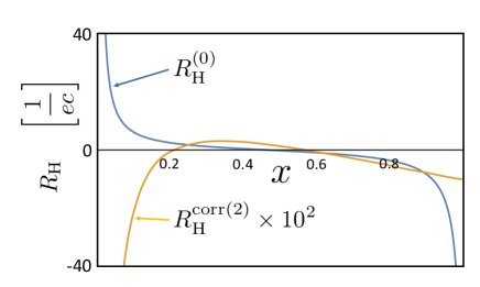
We calculate the correction term up to second order
| (268) |
The three hypermagnetization matrix elements were evaluated numerically. Each application of the Liouvillian or the hypermagnetization can create a new hyperstate by multiplying the individual site operators site-by-site using a multiplication table. The calculation of to leading order in involved traces over up to operator clusters.
In Fig. 18, we plot the final result for for all doping concentrations. We see that in comparison , the its quantitative effect is negligible, and maximized toward by
| (269) |
32 Discussion
Sign reversal of the Hall coefficient at low doping has been previously obtained by dynamical mean field theory (DMFT) [78, 79], QMC [80, 81] and determinant QMC [82]. These methods have found evidence of hole pockets in the momentum dependent occupation, which is qualitatively consistent with our results at low doping. Refs. [83, 84, 85] calculate (within DMFT) the Hall conductivity of the Hubbard model at strong magnetic fields. They found that the Hall sign is reversed relative to band theory, near half filling. These effects were attributed to the Chern numbers of the non-interacting Hofstadter’s butterfly bands of the square lattice. It is interesting that these sign changes which were predicted at strong fields, (as measured in strongly correlated flat bands Moiré systems [86]), are qualitatively similar to the Hall sign we obtain in the weak field limit.
Here however, we find that the sign reversal occurs already at , which may come as a surprise vis-a-vis the widely used band theoretical approaches at much lower doping. The reason is simply related to the spin and charge entangled commutation relations of GP current operators of the tJM,
| (270) |
which affects the hole density dependence of the CMC, and determines the doping concentration of the sign reversal.
Since the hole density operators have coefficients of order unity, it is natural that the sign change occurs at a fraction with a denominator not much larger than unity. The important lesson we can learn from this is that the effects of GP reach far into the high doping and temperature regimes.
Previous QMC calculations of for the HM [80, 87] have used our Eq. (232), and neglected . They have also reported a positive Hall sign near half filling (but no apparent divergence) for the square lattice model. However in the regime of , , is expected to dominate over , and hence cannot be ignored.
We can compare of Eq. (263) to the infinite frequency Hall coefficient of the t-model calculated at leading order in by Shastry, Shriman and Singh [88],
| (271) |
changes sign at and diverges as toward the Mott limit. While Eq. (263) changes sign at and diverges as at small . Still, the qualitative similarity we find between the infinite and zero frequencies is surprising, but we cannot infer any general relations from this coincidence. We note that may be relevant to the optical Kerr effect [89].
In summary, the calculation of the DC Hall coefficient as a function of hole doping in the IT regime appears to be well controlled. We can learn from it that the Mott insulator phase affects the charge carriers in the nearby metallic phase. This has theoretical implication to any possible ordered phases at lower temperatures, such as superconductivity and/or other orders [3, 23, 24, 90]. The superconducting order parameter should consist of GP holes, with spin entangled commutation relations (270), rather than quasiparticles near the non-interacting Fermi surface. The GP also governs the relation between superfluid stiffness (which is bounded by the CSR), and the electron density [91]. It affects the moving vortex charge and the Hall sign in the flux flow regime [92, 93].
Part VIII Strongly Correlated Bosons
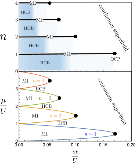
33 The Bose Hubbard model
The Bose Hubbard model (BHM) is a minimal model of interacting lattice bosons,
| (272) |
is the hopping rate and is the local repulsive interaction, is the boson charge, and is the speed of light. The lattice constant is unity. creates a boson on lattice site , and is the boson occupation. , where is the electromagnetic vector potential.
can be realized by cold bosonic atoms trapped in an optical lattice, where can be implemented by light induced artificial gauge fields [94].
The BHM also describe a Josephson junction array where the BCS pairing gap in each grain is larger than the Josephson coupling . would be the inverse capacitance of each grain.
33.1 Weak interactions
We note that for weak interactions, , the bosons condense into the eigenstates with effective dispersion . The low energy theory is therefore effectively a Galilean symmetric continuum theory described by the Gross-Pitaevskii (GP) action [96],
| (273) |
where is a complex coherent-state field which represents the lattice boson operator . For dimension , describes a superconductor at low temperatures, and a charged bosons gas above a finite transition temperature. In the presence of impurities, the metallic conductivity tensor is described by Drude theory Eq. (6) with scattering rate which vanishes with impurity concentration. Therefore by (7), the Hall coefficient is equal to the Galilean symmetric result,
| (274) |
where is the boson density. No Hall sign change is expected at as function of density or temperature in the weak interactions regime.
33.2 Strong interaction
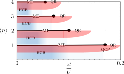
Fig. 20 depicts the BHM ground state Chern number (Eq. (80) as calculated by Huber and Lindner [97] in the strong interaction regime. We note the red regions of Hall sign reversal at strong interactions. While at zero temperature the ground state is a gapless superfluid with zero Hall resistivity, and the Chern calculation should not apply (see Section 13). Nevrtheless, we find that the Hall sign agrees with the Hall coefficient sign in the the corresponding metallic phases at higher temperature, as described below.
For strong interactions, there are Mott insulator lobes in which the boson filling is locked into an integer . The mean field boundaries for the Mott lobe , is given by the implicit equation [99],
| (275) |
which also determines the location of the Quantum Critical Points (QCP) , by the equation .
Near the QCP at density , the BHM maps onto an O(2) quantum field theory [100], described by a complex field . In a dimensionless scaled form [101] the O(2) action is,
| (276) |
is the imaginary time coordinate, . The coupling constant determines ground state. In , , the field theory describes a superconductor, and for it is a Mott insulator. is the QCP. is the bare Higgs (amplitude mode) mass. The low energy Higgs mass and the superfluid stiffness vanish at the QCP.
In order to obtain operator expression for the currents and magnetization, which are necessary for the CMC and CSR susceptibilities, the BHM near the QCP can be renormalized onto an effective Quantum Rotators (QR) Hamiltonian [99],
| (277) |
where
| (278) |
physically describes a Josephson junction array, whose grain capacitance and Josephson couplings are related to the BHM parameters,
| (279) |
Near the QCP, is renormalized down to the low energy superfluid stiffness , as given by the CSR,
| (280) |
vanishes at the QCP as , where is the dimensional correlation length exponent of the O(2) model [17]. also depends on the electron density . Expanding the density fluctuations about the integer Mott density in the path integral, we obtain the operator,
| (281) |
Thus, the renormalized current and magnetization operators involve both phase and density operators
| (282) |
The CMC can be calculated using the cannonical commutations in Eq. (278):
| (283) |
which according to Eq. (305):
| (284) |
which qualitatively agrees with similar expressions found for the reactive Hall constant near a Mott insulator [102], and for the Hall coefficient of a two leg Luttinger-liquid [103]. may be assumed to be small near the QCP since it depdns on current relaxation which scales with the ratio of lattice constant to the longer correlation length.
Since the Mott densities minimize , The Hall coefficient vanishes at extrema of . Near the QCP, changes from negative to positive at the Mott density , since the superfluid stiffness vanishes at the QCP. The switch from (given by Eq. (274) at low densities) to is expected around midpoint between two Mott lobes. This behavior is captured by the Hard Core Bosons model below.
34 Hard Core Bosons on the square lattice
Between consecutive Mott lobes, at temperatures below , there is a superfluid phase with constrained density fluctuations.
These fluctuations can be described by the renormalizing the BHM onto the projected space between two Mott lobes, . The projected charge fluctuations are described hard core bosons (HCB) operators,
| (285) |
These operators are faithfully represented by SU(2) spin-half operators,
| (286) |
which can be used to represent the HCB hamiltonian by the gauged quantum XY model of spin half,
| (287) |
where , which depend on are renormalized from the corresponding BHM values. The HCB charge polarizations, currents and magnetization operators are respectively represented by,
| (288) |
Here denotes the position of site . For the square lattice, the density dependent BKT transition temperature for HCB on the square lattice has been evaluated by QMC: [104, 105, 106]
| (289) |
34.1 Superconducting phase
HCB on the square lattice exhibit long range superfluid order below the Berezinskii, Kosterlitz and Thouless [107, 108] transition (BKT) transition temperature . At the two dimensional superfluid stiffness in the classical (large approximation) is,
| (290) |
which yields a maximum at half filling,
| (291) |
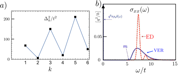
The zero temperature AC longitudinal conductivity at half filling , is evaluated by computing the conductivity moments in Eq. (158) by ED. The resulting 6 recurrents are depicted in Fig. 21(a). The large odd even oscillations of the recurrents indicates that the conductivity is suppressed at low frequencies. In fact, the continuous form of , shown in Fig. 21(a), exhibits a threshold at around . This threshold behavior is supported by an ED calculation for the Kubo formula on a 4 4 lattice.
| (292) |
We note that this threshold feature is not expected by BCS theory in a single band, weak coupling superconductor without disorder. By Mattis and Bardeen [111], such a threshold would appear at , where is the pairing gap only if there is sufficient disorder. For HCB model (287) , and there is no disorder!
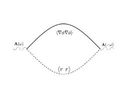
This threshold was argued to be the Higgs-amplitude mode of the particle-hole symmetric Relativistic Gross-Pitaevskii (RGP) theory [17, 101] with Eucledean action,
| (293) |
Here, is the two component rotator field, defined at wavevectors below the cut-off . The imaginary time component is , where , is the microscopic stiffness, and is the local compressibility. is the quantum parameter, which drives a quantum phase transition [99] into a bosonic Mott insulator as it grows toward .
At weak coupling and zero temperature, , and the conductivity is evaluated by fluctuations of the amplitude and phase ,
| (294) |
At lowest order in , the bubble diagram in Fig. 22 yields a threshold AC conductivity given by [101],
| (295) |
where is the mass-gap of the amplitude field . is the analogue of the Higgs particle mass, which vanishes at the critical point with the three dimensional XY model’s correlation length exponent .
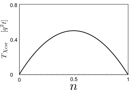
34.2 Metallic phase: longitudinal conductivity
The longitudinal conductivity is evaluated for the metallic phase of on the square lattice, at . The CF expansion is extrapolated following the Variational Extrapolation of Recurrents described in subsection 23.5.
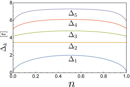
The leading orders CSR is,
| (296) |
were also evaluated to leading order in , which yields recurrents of order . In Fig. 24, the recurrents are plotted for densities .
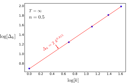
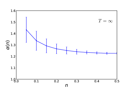
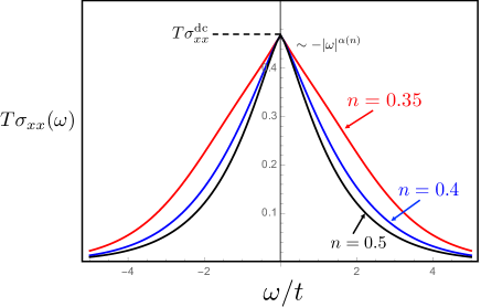
According to (193) and Fig. 7, the termination function appears to be well fit by the stretched exponential form i.e.
| (297) |
where the normalization
| (298) |
ensures that .
The symmetry of the HCB hamiltonian leads to . For , is an outlier of the power law line, since it vanishes as . The higher recurrents are fit by
| (299) |
where is obtained by least square fit in Fig. 26. The error bars increase away from half filling. We find that fluctuations of the recurrents about Eq. (299) induces large uncertainty in th extrapolated . Hence the use of Eq. (299) to the regime .
The high temperature dynamical conductivities are plotted in Fig. 27. Since the first two recurrents are,
| (300) |
The conductivity is proportional to the density independent ratio,
| (301) |
Eq. (301) is interpreted as the ratio of kinetic energy () to scattering rate (), which have a similar density dependence. Hence, since changes very little ( in the range ), the linear resistivity slope in this regime is very weakly density dependent, and given by
| (302) |
The CF extrapolation also yields a singular frequency dependence at low frequencies, as shown in Fig. (27),
| (303) |
The sharp zero frequency cusp is consistent with Mukerjee, Oganesyan, and Huse [112], (MOH) who found a similar singularity in the high temperature conductivity of a one dimensional non-integrable fermion model, and predicted similar behavior in higher dimensional models.
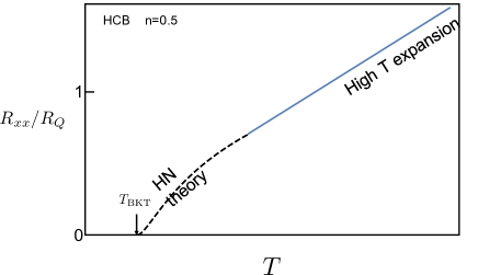
The high temperature linear temperature slope of the HCB resistivity can be connected to the superconducting transition at . Halperin and Nelson (HN) [113] described the superconducting fluctuation region just , where the resitivity rises as
| (304) | |||||
is the BKT correlation length, and is of the order of the HCB lattice constant and . For the HCB model, the “normal state” resistivity is obtained from our Eq. (302). We use these values to plot the crossovers from HN theory Eq. (304) to higher temperatures as dashed lines in Fig. 28.
34.3 Metallic phase: Hall coefficient
The zeroth term,
| (305) |
is calculated by the high temperature expansions of the CSR, Eq. (296) and the CMC susceptibility. The leading order in is,
| (306) | |||||
One observes that () is “particle-hole” symmetric (antisymmetric) under . Thus we obtain,
| (307) |
Notably at low density, the Hall coefficient recovers the continuum Galilean invariant result . Near half-filling, , reflecting the effects of lattice Umklapp and hard core scattering.
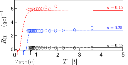
Eq. (307) was extended to lower temperatures numerically [114] by a path-integral based QMC for bosonic lattice models which are devoid of a sign problem. For this purpose, the DSQSS package [115], which employs a path-integral based Monte Carlo scheme for bosons was empoyed, with a Directed Loop Algorithm (DLA) [116]. In Fig. 29, the solid lines are the analytical results of Eq. (307), while the QMC data are depicted by open circles. We see that the Hall coefficients above the HN regime, rapidly saturate to their high temperature limit.
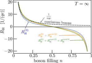
34.4 Hall coefficient corrections
In general, can be a cumbersome calculation. The relative simplicity of the HCB Hamiltonian permits a feasible computation of up to fourth Krylov order. The calculated correction [114] is the truncated sum,
| (308) |
The hypermagnetization matrix elements are calculated as described in Section 28. The fourth order matrix element involved traces over up to operator products. The corrected density dependent high temperature Hall coefficient is depicted in Fig. 30.
We see that these corrections do not qualitatively change the zeroth term’s behavior especially near the densities , although they converge slower around intermediate densities . Since the Hall coefficient is finite for any metal, the summation over higher order corrections must converge. Thus, appears to be qualitatively correct at high temperatures. At lower temperatures , as evaluated by QMC in Fig. 29, appears to be blind to the onset of long range superconducting phase correlations and vortices, as described by HN theory. Therfore toward , the correction term is expected to grow realtive to and cancel it completely at .
35 Discussion
From the calculations shown above, one concludes that near half filling, the ‘weakly interacting continuum bosons’ description fails for HCB. The quantum mechanical effects of lattice periodicity and constraints of no-double occupancies play a crucial role in the transport coefficients.
Part IX Summary and Future Directions
This report reviews recent theoretical advances in quantum transport theory with particular emphasis on application to strongly interacting, gapless phases of matter. The DPP formulas for DC Hall-type conductivities can reduce the computational cost of Kubo formulas in the Lehmann representation. They also help clarify conceptual dilemmas about the role of gapless eigenstates in carrying the Hall currents on OBC, and the ultimate irrelevancy of the magnetization subtractions in thermal Hall conductivities. The DPP formulas generalize the Berry curvature expressions derived in Section 17, for clean non interacting models. This may help us understand the interplay between Berry curvatures and effects of boundaries and disorder [53] within the Kubo formula framework, without appealing to semiclassical approximations.
A significant fraction of this report is devoted to thermodynamic approaches which include continued fractions for AC conductivities, and thermodynamic summation formulas for the electric, thermoelectric and thermal Hall coefficients. These approaches converge better by first renormalizing the Hamiltonian down to the temperature scale of interest, and calculating conductivities which do not consist of separable contributions.
As examples, continued fractions and Hall coefficient summation formulas are applied to basic models of interacting lattice fermions and bosons: the Hubbard, t-J, and HCB Hamiltonians. Conductivities of strongly interacting models are contrasted with their weakly interacting limits in order to illuminate the qualitative effects of strong interactions.
In future studies, thermodynamic approaches can take advantage of reliable variational ground states, e.g. DMRG [3], to obtain low temperature dynamical correlations in other strongly correlated lattice models of spins, fermions and bosons. For example: thermal Hall coefficient formula of strongly frustrated magnetic insulators [60], the Hall conductivity of Heavy fermion metals [118], and nearly ferroelectric material SrTiO4 [119], conductivities of interacting flat band multilayers of graphene [120] and transition metal dichalcoginides [121, 122].
Experimental measurements of conductivities of cold fermionic and bosonic atoms trapped in optical lattices with artifical gauge fields [123] could test the accuracy of thermodynamic calculations. On the mathematical side, further understanding of the relation between low order recurrents and the low frequency behavior of conductivities would be very worthwhile.
36 Acknowledgements
We thank Gil Refael for his encouragement to write the Report. We are indebted to Netanel Lindner, Snir Gazit, Ilia Khait, Noga Bashan, Abhisek Samanta and Ari Turner, whose results are reviewed in this Report. We are grateful for critical comments by Steve Kivelson, Steve Simon, Bruno Uchoa, and Daniel Arovas, which improved the readability of the manuscript. A.A. acknowledges the Israel Science Foundation (ISF) Grant No. 2081/20. This Report was written in part at the Aspen Center for Physics, which is supported by National Science Foundation grant PHY-2210452, and at the Kavli Institute for Theoretical Physics, supported by Grant Nos. NSF PHY-1748958, NSF PHY-1748958 and NSF PHY-2309135.
References
- [1] A. W. Sandvik, Stochastic series expansion method with operator-loop update, Physical Review B 59 (22) (1999) R14157.
-
[2]
N. Prokof’ev, B. Svistunov,
Worm algorithms
for classical statistical models, Phys. Rev. Lett. 87 (2001) 160601.
doi:10.1103/PhysRevLett.87.160601.
URL https://link.aps.org/doi/10.1103/PhysRevLett.87.160601 -
[3]
S. R. White,
Density matrix
formulation for quantum renormalization groups, Phys. Rev. Lett. 69 (1992)
2863–2866.
doi:10.1103/PhysRevLett.69.2863.
URL https://link.aps.org/doi/10.1103/PhysRevLett.69.2863 -
[4]
U. Schollwock,
The
density-matrix renormalization group in the age of matrix product states,
Annals of Physics 326 (1) (2011) 96 – 192, january 2011 Special Issue.
doi:http://dx.doi.org/10.1016/j.aop.2010.09.012.
URL http://www.sciencedirect.com/science/article/pii/S0003491610001752 - [5] P. Corboz, S. R. White, G. Vidal, M. Troyer, Stripes in the two-dimensional t-j model with infinite projected entangled-pair states, Physical Review B 84 (4) (2011) 041108.
- [6] M. Fishman, S. White, E. Stoudenmire, The itensor software library for tensor network calculations, SciPost Physics Codebases (2022) 004.
- [7] W. Kohn, J. Luttinger, Quantum theory of electrical transport phenomena, Physical Review 108 (3) (1957) 590.
- [8] J. Ziman, Electrons and phonons: the theory of transport phenomena in solids, Oxford university press, 1960.
-
[9]
G. Mahan, Many-Particle
Physics, Physics of Solids and Liquids, Springer, 2000.
URL https://books.google.co.il/books?id=xzSgZ4-yyMEC - [10] M. E. Cage, K. Klitzing, A. Chang, F. Duncan, M. Haldane, R. B. Laughlin, A. Pruisken, D. Thouless, The quantum Hall effect, Springer Science & Business Media, 2012.
-
[11]
B. A. Bernevig, Topological
Insulators and Topological Superconductors, Princeton University Press,
Princeton, 2013 [cited 2024-02-20].
doi:doi:10.1515/9781400846733.
URL https://doi.org/10.1515/9781400846733 -
[12]
D. J. Thouless, M. Kohmoto, M. P. Nightingale, M. den Nijs,
Quantized hall
conductance in a two-dimensional periodic potential, Phys. Rev. Lett. 49
(1982) 405–408.
doi:10.1103/PhysRevLett.49.405.
URL https://link.aps.org/doi/10.1103/PhysRevLett.49.405 - [13] J. E. Avron, R. Seiler, Quantization of the hall conductance for general, multiparticle schrödinger hamiltonians, Physical review letters 54 (4) (1985) 259.
-
[14]
P. Streda, L. Smrcka,
Thermodynamic derivation
of the hall current and the thermopower in quantising magnetic field,
Journal of Physics C: Solid State Physics 16 (24) (1983) L895.
URL http://stacks.iop.org/0022-3719/16/i=24/a=005 - [15] . V. Emery, S. Kivelson, Superconductivity in bad metals, Physical Review Letters 74 (16) (1995) 3253.
-
[16]
R. Kubo, Statistical-Mechanical
Theory of Irreversible Processes. I. General Theory and Simple Applications
to Magnetic and Conduction Problems, Journal of the Physical Society of
Japan 12 (6) (1957) 570–586.
arXiv:https://doi.org/10.1143/JPSJ.12.570, doi:10.1143/JPSJ.12.570.
URL https://doi.org/10.1143/JPSJ.12.570 -
[17]
S. Gazit, D. Podolsky, A. Auerbach, D. P. Arovas,
Dynamics and
conductivity near quantum criticality, Phys. Rev. B 88 (2013) 235108.
doi:10.1103/PhysRevB.88.235108.
URL https://link.aps.org/doi/10.1103/PhysRevB.88.235108 -
[18]
N. R. Cooper, B. I. Halperin, I. M. Ruzin,
Thermoelectric
response of an interacting two-dimensional electron gas in a quantizing
magnetic field, Phys. Rev. B 55 (1997) 2344–2359.
doi:10.1103/PhysRevB.55.2344.
URL https://link.aps.org/doi/10.1103/PhysRevB.55.2344 - [19] T. Qin, Q. Niu, J. Shi, Energy magnetization and the thermal hall effect, Physical review letters 107 (23) (2011) 236601.
- [20] N. H. Lindner, A. Auerbach, Conductivity of hard core bosons: A paradigm of a bad metal, Physical Review B 81 (5) (2010) 054512.
- [21] V. Viswanath, G. Müller, The recursion method: application to many body dynamics, Vol. 23, Springer Science & Business Media, 1994.
- [22] I. Khait, S. Bhattacharyya, A. Samanta, A. Auerbach, Hall map and breakdown of fermi liquid theory in the vicinity of a mott insulator, arXiv: 2211.15711 (2022).
-
[23]
S. Sorella, The phase diagram of the
Hubbard model by Variational Auxiliary Field quantum Monte Carlo, Preprint
at: https://arxiv.org/abs/2101.07045 (2021).
doi:10.48550/ARXIV.2101.07045.
URL https://arxiv.org/abs/2101.07045 -
[24]
A. Dorneich, M. Troyer,
Accessing the
dynamics of large many-particle systems using the stochastic series
expansion, Phys. Rev. E 64 (2001) 066701.
doi:10.1103/PhysRevE.64.066701.
URL https://link.aps.org/doi/10.1103/PhysRevE.64.066701 - [25] N. W. Ashcroft, N. D. Mermin, Solid state physics, Cengage Learning, 2022.
- [26] S. M. Girvin, K. Yang, Modern condensed matter physics, Cambridge University Press, 2019.
-
[27]
M.-C. Chang, Q. Niu,
Berry phase,
hyperorbits, and the hofstadter spectrum: Semiclassical dynamics in magnetic
bloch bands, Phys. Rev. B 53 (1996) 7010–7023.
doi:10.1103/PhysRevB.53.7010.
URL https://link.aps.org/doi/10.1103/PhysRevB.53.7010 - [28] H. Mori, Transport, collective motion, and brownian motion, Progress of theoretical physics 33 (3) (1965) 423–455.
- [29] R. Zwanzig, Nonequilibrium statistical mechanics, Oxford university press, 2001.
-
[30]
N. Das, P. Bhalla, N. Singh,
Memory function approach to
correlated electron transport: A comprehensive review, International Journal
of Modern Physics B 30 (23) (2016) 1630015.
arXiv:https://doi.org/10.1142/S0217979216300152, doi:10.1142/S0217979216300152.
URL https://doi.org/10.1142/S0217979216300152 - [31] W. Götze, P. Wölfle, Homogeneous dynamical conductivity of simple metals, Physical Review B 6 (4) (1972) 1226.
-
[32]
P. W. Anderson,
Absence of diffusion
in certain random lattices, Phys. Rev. 109 (1958) 1492–1505.
doi:10.1103/PhysRev.109.1492.
URL https://link.aps.org/doi/10.1103/PhysRev.109.1492 - [33] E. Abrahams, P. Anderson, D. Licciardello, T. Ramakrishnan, Scaling theory of localization: Absence of quantum diffusion in two dimensions, Physical Review Letters 42 (10) (1979) 673.
- [34] E. Abrahams, 50 years of Anderson Localization, Vol. 24, world scientific, 2010.
- [35] E. Akkermans, G. Montambaux, Mesoscopic physics of electrons and photons, Cambridge university press, 2007.
- [36] A. Ioffe, A. Regel, Non-crystalline, amorphous, and liquid electronic semiconductors, Progress in semiconductors (1960) 237–291.
-
[37]
K. T. N. E. Hussey, H. Takagi,
Universality of the
mott-ioffe-regel limit in metals, Philosophical Magazine 84 (27) (2004)
2847–2864.
arXiv:https://doi.org/10.1080/14786430410001716944, doi:10.1080/14786430410001716944.
URL https://doi.org/10.1080/14786430410001716944 -
[38]
P. B. Allen, B. Chakraborty,
Infrared and dc
conductivity in metals with strong scattering: Nonclassical behavior from a
generalized boltzmann equation containing band-mixing effects, Phys. Rev. B
23 (1981) 4815–4827.
doi:10.1103/PhysRevB.23.4815.
URL https://link.aps.org/doi/10.1103/PhysRevB.23.4815 -
[39]
A. Sekine, D. Culcer, A. H. MacDonald,
Quantum kinetic
theory of the chiral anomaly, Phys. Rev. B 96 (2017) 235134.
doi:10.1103/PhysRevB.96.235134.
URL https://link.aps.org/doi/10.1103/PhysRevB.96.235134 -
[40]
C. H. Wong, Y. Tserkovnyak,
Quantum kinetic
equation in phase-space textured multiband systems, Phys. Rev. B 84 (2011)
115209.
doi:10.1103/PhysRevB.84.115209.
URL https://link.aps.org/doi/10.1103/PhysRevB.84.115209 -
[41]
J. M. Luttinger,
Theory of thermal
transport coefficients, Phys. Rev. 135 (1964) A1505–A1514.
doi:10.1103/PhysRev.135.A1505.
URL https://link.aps.org/doi/10.1103/PhysRev.135.A1505 - [42] B. S. Shastry, Sum rule for thermal conductivity and dynamical thermal transport coefficients in condensed matter, Physical Review B 73 (8) (2006) 085117.
- [43] T. Qin, J. Zhou, J. Shi, Berry curvature and the phonon hall effect, Physical Review B 86 (10) (2012) 104305.
- [44] H. Katsura, N. Nagaosa, P. A. Lee, Theory of the thermal hall effect in quantum magnets, Physical review letters 104 (6) (2010) 066403.
-
[45]
S. H. Simon, M. S. Rudner,
Contrasting
lattice geometry dependent versus independent quantities: Ramifications for
berry curvature, energy gaps, and dynamics, Phys. Rev. B 102 (2020) 165148.
doi:10.1103/PhysRevB.102.165148.
URL https://link.aps.org/doi/10.1103/PhysRevB.102.165148 - [46] F. D. M. Haldane, Model for a quantum hall effect without landau levels: Condensed-matter realization of the” parity anomaly”, Physical review letters 61 (18) (1988) 2015.
- [47] A. Auerbach, Equilibrium formulae for transverse magnetotransport of strongly correlated metals, Physical Review B 99 (11) (2019) 115115.
- [48] A. Yacoby, H. Hess, T. Fulton, L. Pfeiffer, K. West, Electrical imaging of the quantum hall state, Solid state communications 111 (1) (1999) 1–13.
-
[49]
D. Xiao, Y. Yao, Z. Fang, Q. Niu,
Berry-phase
effect in anomalous thermoelectric transport, Phys. Rev. Lett. 97 (2006)
026603.
doi:10.1103/PhysRevLett.97.026603.
URL https://link.aps.org/doi/10.1103/PhysRevLett.97.026603 -
[50]
R. Matsumoto, S. Murakami,
Rotational motion
of magnons and the thermal hall effect, Phys. Rev. B 84 (2011) 184406.
doi:10.1103/PhysRevB.84.184406.
URL https://link.aps.org/doi/10.1103/PhysRevB.84.184406 -
[51]
G. Sundaram, Q. Niu,
Wave-packet
dynamics in slowly perturbed crystals: Gradient corrections and berry-phase
effects, Phys. Rev. B 59 (1999) 14915–14925.
doi:10.1103/PhysRevB.59.14915.
URL https://link.aps.org/doi/10.1103/PhysRevB.59.14915 - [52] T. Jungwirth, Q. Niu, A. MacDonald, Anomalous hall effect in ferromagnetic semiconductors, Physical review letters 88 (20) (2002) 207208.
- [53] N. Sinitsyn, Q. Niu, J. Sinova, K. Nomura, Disorder effects in the anomalous hall effect induced by berry curvature, Physical Review B 72 (4) (2005) 045346.
- [54] M. P. Marder, Condensed matter physics, John Wiley & Sons, 2010.
-
[55]
J.-i. Inoue, G. E. W. Bauer, L. W. Molenkamp,
Suppression of the
persistent spin hall current by defect scattering, Phys. Rev. B 70 (2004)
041303.
doi:10.1103/PhysRevB.70.041303.
URL https://link.aps.org/doi/10.1103/PhysRevB.70.041303 - [56] K. Nomura, J. Sinova, T. Jungwirth, Q. Niu, A. MacDonald, Nonvanishing spin hall currents in disordered spin-orbit coupling systems, Physical Review B 71 (4) (2005) 041304.
- [57] A. Shytov, E. Mishchenko, H.-A. Engel, B. Halperin, Small-angle impurity scattering and the spin hall conductivity in two-dimensional semiconductor systems, Physical Review B 73 (7) (2006) 075316.
- [58] N. Bashan, A. Auerbach, Degeneracy-projected polarization formulas for hall-type conductivities, Physical Review Letters 128 (3) (2022) 036601.
- [59] J. Chalker, P. Coddington, Percolation, quantum tunnelling and the integer hall effect, Journal of Physics C: Solid State Physics 21 (14) (1988) 2665.
-
[60]
Y. Kasahara, K. Sugii, T. Ohnishi, M. Shimozawa, M. Yamashita, N. Kurita,
H. Tanaka, J. Nasu, Y. Motome, T. Shibauchi, Y. Matsuda,
Unusual
thermal hall effect in a kitaev spin liquid candidate
, Phys. Rev.
Lett. 120 (2018) 217205.
doi:10.1103/PhysRevLett.120.217205.
URL https://link.aps.org/doi/10.1103/PhysRevLett.120.217205 - [61] X. Li, B. Fauqué, Z. Zhu, K. Behnia, Phonon thermal Hall effect in strontium titanate, Physical review letters 124 (10) (2020) 105901.
-
[62]
G. Grissonnanche, S. Thériault, A. Gourgout, M. E. Boulanger, E. Lefrançois, A. Ataei, F. Laliberté, M. Dion, J. S. Zhou, S. Pyon, T. Takayama,
H. Takagi, N. Doiron-Leyraud, L. Taillefer,
Chiral phonons in the
pseudogap phase of cuprates, Nature Physics 16 (11) (2020) 1108–1111.
doi:10.1038/s41567-020-0965-y.
URL https://doi.org/10.1038/s41567-020-0965-y - [63] R. P. Feynman, Atomic theory of the two-fluid model of liquid helium, Physical Review 94 (2) (1954) 262.
-
[64]
S. M. Girvin, A. H. MacDonald, P. M. Platzman,
Magneto-roton theory
of collective excitations in the fractional quantum hall effect, Phys. Rev.
B 33 (1986) 2481–2494.
doi:10.1103/PhysRevB.33.2481.
URL https://link.aps.org/doi/10.1103/PhysRevB.33.2481 - [65] D. P. Arovas, A. Auerbach, F. Haldane, Extended heisenberg models of antiferromagnetism: Analogies to the fractional quantum hall effect, Physical review letters 60 (6) (1988) 531.
- [66] A. Auerbach, Interacting electrons and quantum magnetism, Springer Science & Business Media, 2012.
- [67] G. Freud, On the coefficients in the recursion formulae of orthogonal polynomials, in: Proceedings of the Royal Irish Academy. Section A: Mathematical and Physical Sciences, JSTOR, 1976, pp. 1–6.
- [68] D. Lubinsky, H. Mhaskar, E. Saff, A proof of freud’s conjecture for exponential weights, Constructive Approximation 4 (1988) 65–83.
- [69] A. Auerbach, Hall number of strongly correlated metals, Physical Review Letters 121 (6) (2018) 066601.
- [70] N. Lindner, A. Auerbach, D. P. Arovas, Vortex dynamics and hall conductivity of hard-core bosons, Physical Review B 82 (13) (2010) 134510.
- [71] A. Samanta, D. P. Arovas, A. Auerbach, Hall coefficient of semimetals, Physical Review Letters 126 (7) (2021) 076603.
-
[72]
J. Hubbard, Electron correlations
in narrow energy bands, Proc. R. Soc. Lond. (1963).
doi:10.1103/PhysRevLett.111.036401.
URL http://doi.org/10.1098/rspa.1963.0204 -
[73]
D. P. Arovas, E. Berg, S. A. Kivelson, S. Raghu,
The hubbard
model, Annual Review of Condensed Matter Physics 13 (1) (2022) 239–274.
arXiv:https://doi.org/10.1146/annurev-conmatphys-031620-102024,
doi:10.1146/annurev-conmatphys-031620-102024.
URL https://doi.org/10.1146/annurev-conmatphys-031620-102024 -
[74]
J. Spałek, Effect
of pair hopping and magnitude of intra-atomic interaction on
exchange-mediated superconductivity, Phys. Rev. B 37 (1988) 533–536.
doi:10.1103/PhysRevB.37.533.
URL https://link.aps.org/doi/10.1103/PhysRevB.37.533 - [75] J. Jaklič, P. Prelovšek, Charge dynamics in the planar t-J model, Physical Review B 52 (9) (1995) 6903.
- [76] E. Perepelitsky, A. Galatas, J. Mravlje, E. Khatami, B. S. Shastry, A. Georges, et al., Transport and optical conductivity in the Hubbard model: A high-temperature expansion perspective, Physical Review B 94 (23) (2016) 235115.
-
[77]
E. W. Huang, R. Sheppard, B. Moritz, T. P. Devereaux,
Strange
metallicity in the doped hubbard model, Science 366 (6468) (2019) 987–990.
arXiv:https://www.science.org/doi/pdf/10.1126/science.aau7063, doi:10.1126/science.aau7063.
URL https://www.science.org/doi/abs/10.1126/science.aau7063 -
[78]
W. Xu, K. Haule, G. Kotliar,
Hidden Fermi
Liquid, Scattering Rate Saturation, and Nernst Effect: A Dynamical Mean-Field
Theory Perspective, Phys. Rev. Lett. 111 (2013) 036401.
doi:10.1103/PhysRevLett.111.036401.
URL https://link.aps.org/doi/10.1103/PhysRevLett.111.036401 - [79] E. Z. Kuchinskii, N. A. Kuleeva, D. I. Khomskii, M. V. Sadovskii, Hall effect in a doped mott insulator: Dmft approximation, JETP Letters 115 (7) (2022) 402–405.
-
[80]
W. O. Wang, J. K. Ding, B. Moritz, Y. Schattner, E. W. Huang, T. P. Devereaux,
Numerical
approaches for calculating the low-field dc Hall coefficient of the doped
Hubbard model, Phys. Rev. Research 3 (2021) 033033.
doi:10.1103/PhysRevResearch.3.033033.
URL https://link.aps.org/doi/10.1103/PhysRevResearch.3.033033 - [81] Imaginary time QMC conductivities require analytic continuation, which is limited to frequencies higher than temperature (see Appendix B in [17]). The DC conductivities are often deduced by proxies to the analytical continuation [80].
-
[82]
W. Wu, M. S. Scheurer, S. Chatterjee, S. Sachdev, A. Georges, M. Ferrero,
Pseudogap and
fermi-surface topology in the two-dimensional hubbard model, Phys. Rev. X 8
(2018) 021048.
doi:10.1103/PhysRevX.8.021048.
URL https://link.aps.org/doi/10.1103/PhysRevX.8.021048 -
[83]
A. A. Markov, G. Rohringer, A. N. Rubtsov,
Robustness of
the topological quantization of the Hall conductivity for correlated lattice
electrons at finite temperatures, Phys. Rev. B 100 (2019) 115102.
doi:10.1103/PhysRevB.100.115102.
URL https://link.aps.org/doi/10.1103/PhysRevB.100.115102 -
[84]
J. Vučičević, R. Žitko,
Electrical
conductivity in the Hubbard model: Orbital effects of magnetic field, Phys.
Rev. B 104 (2021) 205101.
doi:10.1103/PhysRevB.104.205101.
URL https://link.aps.org/doi/10.1103/PhysRevB.104.205101 - [85] Y. Shi, J. Schirmer, L.-Q. Chen, Hall coefficient and resistivity in the doped bilayer hubbard model, Preprint at: https://arxiv.org/abs/2308.03862 (2023).
- [86] R. Krishna Kumar, X. Chen, G. Auton, A. Mishchenko, D. A. Bandurin, S. V. Morozov, Y. Cao, E. Khestanova, M. Ben Shalom, A. Kretinin, et al., High-temperature quantum oscillations caused by recurring Bloch states in graphene superlattices, Science 357 (6347) (2017) 181–184.
- [87] W. O. Wang, J. K. Ding, B. Moritz, E. W. Huang, T. P. Devereaux, Dc hall coefficient of the strongly correlated hubbard model, npj Quantum Materials 5 (1) (2020) 51.
- [88] B. Shastry, B. Shraiman, R. Singh, Faraday rotation and the hall constant in strongly correlated fermi systems, Physical review letters 70 (13) (1993) 2004.
-
[89]
P. Hosur, A. Kapitulnik, S. A. Kivelson, J. Orenstein, S. Raghu, W. Cho,
A. Fried,
Erratum: Kerr
effect as evidence of gyrotropic order in the cuprates [Phys. Rev. B 87,
115116 (2013)], Phys. Rev. B 91 (2015) 039908.
doi:10.1103/PhysRevB.91.039908.
URL https://link.aps.org/doi/10.1103/PhysRevB.91.039908 -
[90]
P. W. Anderson,
The
Resonating Valence Bond State in LaCuO and Superconductivity, Science
235 (4793) (1987) 1196–1198.
arXiv:https://www.science.org/doi/pdf/10.1126/science.235.4793.1196,
doi:10.1126/science.235.4793.1196.
URL https://www.science.org/doi/abs/10.1126/science.235.4793.1196 -
[91]
Y. J. Uemura, G. M. Luke, B. J. Sternlieb, J. H. Brewer, J. F. Carolan, W. N.
Hardy, R. Kadono, J. R. Kempton, R. F. Kiefl, S. R. Kreitzman, P. Mulhern,
T. M. Riseman, D. L. Williams, B. X. Yang, S. Uchida, H. Takagi,
J. Gopalakrishnan, A. W. Sleight, M. A. Subramanian, C. L. Chien, M. Z.
Cieplak, G. Xiao, V. Y. Lee, B. W. Statt, C. E. Stronach, W. J. Kossler,
X. H. Yu,
Universal
Correlations between and (Carrier Density
over Effective Mass) in High- Cuprate Superconductors, Phys. Rev.
Lett. 62 (1989) 2317–2320.
doi:10.1103/PhysRevLett.62.2317.
URL https://link.aps.org/doi/10.1103/PhysRevLett.62.2317 -
[92]
S. Y. F. Zhao, N. Poccia, M. G. Panetta, C. Yu, J. W. Johnson, H. Yoo,
R. Zhong, G. D. Gu, K. Watanabe, T. Taniguchi, S. V. Postolova, V. M.
Vinokur, P. Kim,
Sign-Reversing
Hall Effect in Atomically Thin High-Temperature
Superconductors, Phys. Rev. Lett. 122 (2019) 247001.
doi:10.1103/PhysRevLett.122.247001.
URL https://link.aps.org/doi/10.1103/PhysRevLett.122.247001 -
[93]
A. Auerbach, D. P. Arovas,
Hall anomaly and
moving vortex charge in layered superconductors, SciPost Phys. 8 (2020)
061.
doi:10.21468/SciPostPhys.8.4.061.
URL https://scipost.org/10.21468/SciPostPhys.8.4.061 -
[94]
Y. J. Lin, R. L. Compton, K. Jiménez-García, J. V. Porto, I. B.
Spielman, Synthetic magnetic
fields for ultracold neutral atoms, Nature 462 (7273) (2009) 628–632.
doi:10.1038/nature08609.
URL https://doi.org/10.1038/nature08609 - [95] R. T. Scalettar, G. G. Batrouni, G. T. Zimanyi, Localization in interacting, disordered, bose systems, Physical review letters 66 (24) (1991) 3144.
- [96] L. Pitaevskii, S. Stringari, Bose-Einstein condensation and superfluidity, Vol. 164, Oxford University Press, 2016.
- [97] S. D. Huber, N. H. Lindner, Topological transitions for lattice bosons in a magnetic field, Proceedings of the National Academy of Sciences 108 (50) (2011) 19925–19930.
- [98] N. H. Lindner, A. Auerbach, D. P. Arovas, Vortex quantum dynamics of two dimensional lattice bosons, Physical review letters 102 (7) (2009) 070403.
- [99] S. Sachdev, Quantum phase transitions, second ed. Edition, Cambridge University Press, Cambridge, 2011.
- [100] M. P. Fisher, P. B. Weichman, G. Grinstein, D. S. Fisher, Boson localization and the superfluid-insulator transition, Physical Review B 40 (1) (1989) 546.
- [101] D. Podolsky, A. Auerbach, D. P. Arovas, Visibility of the amplitude (higgs) mode in condensed matter, Physical Review B 84 (17) (2011) 174522.
- [102] X. Zotos, F. Naef, M. Long, P. Prelovšek, Drude Weight, Integrable Systems and the Reactive Hall Constant, Springer Netherlands, Dordrecht, 2001, pp. 273–282.
- [103] R. Citro, T. Giamarchi, E. Orignac, Hall response in interacting bosonic and fermionic ladders (2024). arXiv:2404.16973.
- [104] H.-Q. Ding, M. Makivic, Kosterlitz-thouless transition in the two-dimensional quantum xy model, Physical Review B 42 (10) (1990) 6827.
-
[105]
H.-Q. Ding, Phase
transition and thermodynamics of quantum xy model in two dimensions, Phys.
Rev. B 45 (1992) 230–242.
doi:10.1103/PhysRevB.45.230.
URL https://link.aps.org/doi/10.1103/PhysRevB.45.230 -
[106]
K. Harada, N. Kawashima,
Universal jump in
the helicity modulus of the two-dimensional quantum xy model, Phys. Rev. B
55 (1997) R11949–R11952.
doi:10.1103/PhysRevB.55.R11949.
URL https://link.aps.org/doi/10.1103/PhysRevB.55.R11949 - [107] V. Berezinskii, Destruction of long-range order in one-dimensional and two-dimensional systems having a continuous symmetry group i. classical systems, Sov. Phys. JETP 32 (3) (1971) 493–500.
- [108] J. M. Kosterlitz, D. J. Thouless, Ordering, metastability and phase transitions in two-dimensional systems, Journal of Physics C: Solid State Physics 6 (7) (1973) 1181.
- [109] A. W. Sandvik, C. J. Hamer, Ground-state parameters, finite-size scaling, and low-temperature properties of the two-dimensional s= 1 2 xy model, Physical Review B 60 (9) (1999) 6588.
- [110] K. Bernardet, G. Batrouni, J.-L. Meunier, G. Schmid, M. Troyer, A. Dorneich, Analytical and numerical study of hardcore bosons in two dimensions, Physical Review B 65 (10) (2002) 104519.
- [111] D. C. Mattis, J. Bardeen, Theory of the anomalous skin effect in normal and superconducting metals, Physical Review 111 (2) (1958) 412.
- [112] S. Mukerjee, V. Oganesyan, D. Huse, Statistical theory of transport by strongly interacting lattice fermions, Physical Review B 73 (3) (2006) 035113.
- [113] B. Halperin, D. R. Nelson, Resistive transition in superconducting films, Journal of low temperature physics 36 (1979) 599–616.
- [114] S. Bhattacharyya, A. De, S. Gazit, A. Auerbach, Metallic transport of hard core bosons, arXiv:2309.14479 (2023). arXiv:2309.14479.
-
[115]
Y. Motoyama, K. Yoshimi, A. Masaki-Kato, T. Kato, N. Kawashima,
Dsqss:
Discrete space quantum systems solver, Computer Physics Communications 264
(2021) 107944.
doi:https://doi.org/10.1016/j.cpc.2021.107944.
URL https://www.sciencedirect.com/science/article/pii/S0010465521000692 -
[116]
O. F. Syljuåsen, A. W. Sandvik,
Quantum monte
carlo with directed loops, Phys. Rev. E 66 (2002) 046701.
doi:10.1103/PhysRevE.66.046701.
URL https://link.aps.org/doi/10.1103/PhysRevE.66.046701 - [117] I. Khait, S. Bhattacharyya, A. Samanta, A. Auerbach, Hall map and breakdown of Fermi liquid theory in the vicinity of a Mott insulator, arXiv:2211.15711 (2022).
- [118] N. Maksimovic, D. H. Eilbott, T. Cookmeyer, F. Wan, J. Rusz, V. Nagarajan, S. C. Haley, E. Maniv, A. Gong, S. Faubel, I. M. Hayes, A. Bangura, J. Singleton, J. C. Palmstrom, L. Winter, R. McDonald, S. Jang, P. Ai, Y. Lin, S. Ciocys, J. Gobbo, Y. Werman, P. M. Oppeneer, E. Altman, A. Lanzara, J. G. Analytis, Evidence for a delocalization quantum phase transition without symmetry breaking in CeCoIn, Science 375 (6576) (2022) 76–81. arXiv:https://www.science.org/doi/pdf/10.1126/science.aaz4566, doi:10.1126/science.aaz4566.
- [119] X. Li, B. Fauqué, Z. Zhu, K. Behnia, Phonon thermal Hall effect in strontium titanate, Physical review letters 124 (10) (2020) 105901.
-
[120]
E. Y. Andrei, A. H. MacDonald,
Graphene bilayers with a
twist, Nature Materials 19 (12) (2020) 1265–1275.
doi:10.1038/s41563-020-00840-0.
URL https://doi.org/10.1038/s41563-020-00840-0 -
[121]
M. M. Scherer, D. M. Kennes, L. Classen,
Chiral superconductivity
with enhanced quantized Hall responses in moiré transition metal
dichalcogenides, npj Quantum Materials 7 (1) (2022) 100.
doi:10.1038/s41535-022-00504-z.
URL https://doi.org/10.1038/s41535-022-00504-z -
[122]
J. Pizarro, S. Adler, K. Zantout, T. Mertz, P. Barone, R. Valentí,
G. Sangiovanni, T. O. Wehling,
Deconfinement of Mott
localized electrons into topological and spin–orbit-coupled Dirac
fermions, npj Quantum Materials 5 (1) (2020) 79.
doi:10.1038/s41535-020-00277-3.
URL https://doi.org/10.1038/s41535-020-00277-3 - [123] P. T. Brown, D. Mitra, E. Guardado-Sanchez, R. Nourafkan, A. Reymbaut, C.-D. Hébert, S. Bergeron, A.-M. Tremblay, J. Kokalj, D. A. Huse, et al., Bad metallic transport in a cold atom Fermi-Hubbard system, Science 363 (6425) (2019) 379–382.