A new standard for the logarithmic accuracy of parton showers

Abstract

We report on a major milestone in the construction of logarithmically accurate final-state parton showers, achieving next-to-next-to-leading-logarithmic (NNLL) accuracy for the wide class of observables known as event shapes. The key to this advance lies in the identification of the relation between critical NNLL analytic resummation ingredients and their parton-shower counterparts. Our analytic discussion is supplemented with numerical tests of the logarithmic accuracy of three shower variants for more than a dozen distinct event-shape observables in $Z\to q\bar{q}$ and Higgs $\to gg$ decays. The NNLL terms are phenomenologically sizeable, as illustrated in comparisons to data.

Parton showers are essential tools for predicting QCD physics at colliders across a wide range of momenta from the TeV down to the GeV regime [1, 2, 3, 4]. In the presence of such disparate momenta, the perturbative expansions of quantum field theories have coefficients enhanced by large logarithms of the ratios of momentum scales. One way of viewing parton showers is as automated and immensely flexible tools for resumming those logarithms, thus correctly reproducing the corresponding physics.

The accuracy of resummations is usually classified based on terms with the greatest logarithmic power at each order in the strong coupling (leading logarithms or LL), and then towers of terms with subleading powers of logarithms at each order in the coupling (next-to-leading logarithms or NLL, NNLL, etc.). Higher logarithmic accuracy for parton showers should make them considerably more powerful tools for analysing and interpreting experimental data at CERN’s Large Hadron Collider and potential future colliders. The past years have seen major breakthroughs in advancing the logarithmic accuracy of parton showers, with several groups taking colour-dipole showers from LL to NLL [5, 6, 7, 8, 9, 10, 11, 12, 13, 14, 15, 16, 17, 18]. There has also been extensive work on incorporating higher-order splitting kernels into showers [19, 20, 21, 22, 23, 24, 25, 26, 27, 28, 29] and understanding the structure of subleading-colour corrections, see e.g. Refs. [30, 31, 32, 33, 34, 35, 6, 36, 37, 38, 39, 40, 41].

Here, for the first time, we show how to construct parton showers with NNLL accuracy for the broad class of event-shape observables at lepton colliders, like the well-known Thrust [42, 43] (see e.g. Refs. [44, 45, 46, 47, 48, 49, 50, 51, 52, 53, 54, 55, 56, 57, 58, 59, 60, 61, 62, 63, 64, 65] for calculations at NNLL and beyond). This is achieved by developing a novel framework that unifies several recent developments, on (a) the inclusive structure of soft-collinear gluon emission [58, 66] up to third order in the strong coupling $\alpha_{s}$; (b) the inclusive pattern of energetic (“hard”) collinear radiation up to order $\alpha_{s}^{2}$ [67, 68]; and (c) the incorporation of soft radiation fully differentially up to order $\alpha_{s}^{2}$ in parton showers, ensuring correct generation of any number of well-separated pairs of soft emissions [29].

We will focus the discussion on the $e^{+}e^{-}\to Z\to q\bar{q}$ process, with the understanding that the same arguments apply also to $H\to gg$. Each event has a set of emissions with momenta $\{k_{i}\}$ and we work in units where the centre-of-mass energy $Q\equiv 1$. We will examine the probability $\Sigma(v)$ that some global event shape, $V(\{k_{i}\})$, has a value $V(\{k_{i}\})<v$. Event-shape observables have the property [69] that for a single soft and collinear emission $k$, $V(k)\propto k_{t}e^{-\beta_{\text{obs}}|y|}$, where $k_{t}$ ($y$) is the transverse momentum (rapidity) of $k$ with respect to the Born event direction and $\beta_{\text{obs}}$ depends on the specific observable, e.g. $\beta_{\text{obs}}=1$ for Thrust. Whether considering analytic resummation or a parton shower, for $v\ll 1$ we have

$$\Sigma(v)\!=\!\mathcal{F}\exp\!\left[\!-4\!\!\int\!\frac{dk_{t}}{k_{t}}\!\!\int_{k_{t}}^{1}\!\!\!\!dzP_{\!gq}(z)M(k)\frac{\alpha_{\text{eff}}}{2\pi}\Theta(V(k)\!>\!v)\right]\!\!,$$ (1)

with $P_{gq}(z)=C_{F}\frac{1+(1-z)^{2}}{z}$ and $M(k)$ a function that accounts for next-to-leading order matching, with $M(k)\to 1$ for $k_{t}\to 0$. The exponential is a Sudakov form factor, encoding the suppression of emissions with $V(k)>v$, cf. the grey region of Fig. 1. It brings the LL contributions to $\ln\Sigma$, terms $\alpha_{s}^{n}L^{n+1}$ with $L=\ln v$, as well as NLL ($\alpha_{s}^{n}L^{n}$), NNLL ($\alpha_{s}^{n}L^{n-1}$), etc., contributions. The function $\mathcal{F}$ accounts [69] for the difference between the actual condition $V(\{k_{i}\})<v$ and the simplified single-emission boundary $V(k)<v$ that is used in the Sudakov. It starts at NLL.

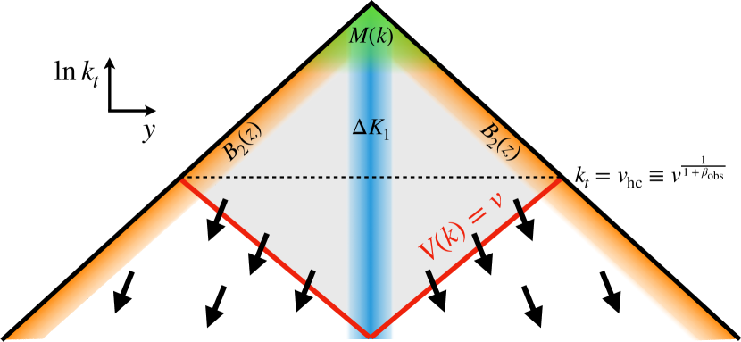
Figure 1: Schematic representation of the Lund plane [70]. A constraint on an event shape that scales as $k_{t}e^{-\beta_{\text{obs}}|y|}$ implies that shower emissions above the red line are mostly vetoed. At NNLL, one mechanism that modifies this constraint is that subsequent branching may cause the effective transverse momentum or rapidity to shift, as represented by the arrows.

In Eq. (1), the effective coupling, $\alpha_{\text{eff}}$, can be understood as the intensity of gluon emission, inclusive over possible subsequent branchings of that emission and corresponding virtual corrections. We write it as

$$\alpha_{\text{eff}}=\alpha_{s}\!\left[1\!+\frac{\alpha_{s}}{2\pi}\left(K_{1}\!+\!\Delta K_{1}(y)\!+\!B_{2}(z)\right)+\frac{\alpha_{s}^{2}}{4\pi^{2}}K_{2}\right]\!\!,$$ (2)

with $\alpha_{s}\equiv\alpha_{s}^{\overline{\textsc{ms}}}(k_{t})$ and here the rapidity $y=\ln z/k_{t}$. $K_{1}=(\frac{67}{18}-\frac{\pi^{2}}{6})C_{A}-\frac{10}{9}n_{f}T_{R}$ (often called $K_{\text{{cmw}}}$) [71] is required for NLL accuracy and the remaining terms for NNLL. $\Delta K_{1}(y)$ is zero in the resummation literature, non-zero at central rapidities for certain showers, and vanishes for $y\to\infty$ [29]; $B_{2}(z)$ affects the hard-collinear region and tends to zero in the soft limit, $z\to 0$. In analytic resummation it is generally included as a constant multiplying $\delta(1-z)$ [44]. It has been calculated in specific resummation schemes in Refs. [67, 68], but is not yet known for the showers that we consider, which also do not yet include the relevant triple-collinear dynamics. At NNLL, $K_{2}$ is relevant in the whole soft-collinear region and also so far calculated only for analytic resummation [58, 66]. Through shower unitarity, $\alpha_{\text{eff}}$ is relevant also in the Sudakov-veto region of Fig. 1, i.e. the region above the red line, even though that region contains no emissions or subsequent branching.

It is straightforward to see from Eq. (1) that terms up to $\alpha_{s}^{n}L^{n-1}$ in $\ln\Sigma(v)$ depend only on the integrals of $\Delta K_{1}(y)$ and $B_{2}(z)$,

$$\Delta K_{1}^{\text{int}}\equiv\!\int_{-\infty}^{\infty}\!\!\!\!\!dy\,\Delta K_{1}(y)\,,\,\,B_{2}^{\text{int}}\equiv\!\int_{0}^{1}dz\frac{P_{gq}(z)}{2C_{F}}B_{2}(z).$$ (3)

One of the key observations of this Letter is that as long as a parton shower correctly generates double-soft emissions in the soft-collinear region, it is possible to identify relations between the $\Delta K_{1}^{\text{int}}$, $B_{2}^{\text{int}}$ and $K_{2}$ as relevant for an NNLL event-shape resummation and the corresponding constants needed for a parton shower. This holds even if the shower does not reproduce the full relevant physics at second order in the large-angle and hard-collinear regions and at third order in the soft-collinear region. This is in analogy with the fact that including the correct $K_{1}$ constant is sufficient to obtain NLL accuracy even without the real double-soft contribution.

In the next few paragraphs we will identify the relations between individual resummation and shower ingredients (neglecting terms beyond NNLL), and then show how they combine to achieve overall NNLL shower accuracy. Let us start by recalling how the $\mathcal{O}\left(\alpha_{s}^{2}\right)$ terms of Eq. (2) come about. Consider a Born squared matrix element, $\mathcal{B}_{\tilde{\imath}}$, for producing a gluon ${\tilde{\imath}}$ (multiplied by $\alpha_{s}/2\pi$). Schematically the $\mathcal{O}\left(\alpha_{s}^{2}\right)$ terms involve the single-emission virtual correction $\mathcal{V}_{{\tilde{\imath}}}$ and an integral over a real ${\tilde{\imath}}\to ij$ branching phase space and matrix element, $d\Phi_{ij|{\tilde{\imath}}}\mathcal{R}_{ij}$ (both multiply $(\alpha_{s}/2\pi)^{2}$). The key difference between a resummation calculation and a parton shower lies in the phase-space mapping that is encoded in $d\Phi_{ij|{\tilde{\imath}}}$. For example, in many resummation calculations $g_{\tilde{\imath}}\to q_{i}\bar{q}_{j}$ splitting implicitly conserves transverse momentum ${k}_{t,i+j}={k}_{t{\tilde{\imath}}}$ and rapidity $y_{i+j}=y_{{\tilde{\imath}}}$ with respect to the particle that emitted ${\tilde{\imath}}$ [58, 66]. A parton shower (ps) will organise the phase space differently, and in a way that does not conserve these kinematic quantities. The difference can be represented as an effective drift in one or more kinematic variables $x$ (e.g. $x\equiv\ln k_{t}$, $x\equiv y$) of post- versus pre-branching kinematics. The average drifts, $\frac{\alpha_{s}}{2\pi}\langle\Delta_{x}\rangle$, are represented as arrows in Fig. 1. For a soft-collinear (SC) gluon $k_{\tilde{\imath}}$, they are independent of the kinematics of $k_{\tilde{\imath}}$. For the $C_{F}C_{A}$ and $C_{F}n_{f}$ colour channels they read

$$\langle\Delta_{x}\rangle=\lim_{{\tilde{\imath}}\to\text{{sc}}}\frac{1}{\mathcal{B}_{\tilde{\imath}}}\int d\Phi_{ij|{\tilde{\imath}}}^{\text{{ps}}}\,\mathcal{R}_{ij}\times(x_{i+j}-x_{\tilde{\imath}})\,.$$ (4)

For the $C_{F}^{2}$ channel, one replaces $x_{i+j}$ with the $x$ value of that of $i$ and $j$ that corresponds to the larger shower ordering variable ($v_{\text{{ps}}}=k_{t}e^{-\beta_{\text{{ps}}}|y|}$). Note that the sign of $\langle\Delta_{y}\rangle$ depends on the sign of $y_{\tilde{\imath}}$ (below, $y_{\tilde{\imath}}>0$).

To understand the relation of $\langle\Delta_{y}\rangle$ with $\Delta K^{\text{int}}_{1}$, observe that a drift to large absolute rapidities depletes radiation at central rapidities. However the shower must correctly reproduce the total final amount of radiation integrated over any rapidity window. That can only be achieved with a value for $\Delta K^{\text{int}}_{1}$ that generates just enough extra central radiation to compensate for the drift-induced depletion. Quantitatively, the following relation can be proven (Ref. [72], §.1)

$$\Delta K_{1}^{\text{int,\text{{ps}}}}=2\langle\Delta_{y}\rangle\,.$$ (5)

As a numerical check, Table 1 shows the result of $\Delta K_{1}^{\text{int,\text{{ps}}}}$ as determined in Ref. [29], compared to $\langle\Delta_{y}\rangle$ as determined for this paper. The results are given for three variants [5, 29] of the PanGlobal shower. The $\text{PG}_{\beta=0}$ and $\text{PG}_{\beta=0}^{\text{sdf}}$ showers have $\beta_{\text{{ps}}}=0$ and differ in how the splitting probabilities are assigned between the two dipole ends. For all three variants, one observes good agreement between $\Delta K_{1}^{\text{int,\text{{ps}}}}$ and $2\langle\Delta_{y}\rangle$.

shower	colour	$\frac{1}{4\pi}\Delta K_{1}^{\text{int,\text{{ps}}}}$		$\frac{1}{2\pi}\langle\Delta_{y}\rangle$		$\frac{1}{2\pi}\langle\Delta_{\ln k_{t}}\rangle$
	$C_{F}$	0		0.	000018(39)	-1.	953481(1)
PG${}_{\beta=0}^{\text{sdf}}$	$C_{A}$	0		0.	000002(2)	1.	162602(2)
	$n_{f}T_{R}$	0		-0.	0000003(3)	-0.	1048049(3)
	$C_{F}$	0.	04967(3)	0.	049576(8)	-1.	964624(6)
PGβ=0	$C_{A}$	0.	0323(5)	0.	032107(4)	1.	174900(4)
	$n_{f}T_{R}$	0.	0040(1)	0.	003962(1)	-0.	104655(1)
	$C_{F}$	1.	6725(5)	1.	672942(9)	-1.	749920(5)
PG${}_{\beta=\frac{1}{2}}$	$C_{A}$	0.	0172(11)	0.	015303(5)	1.	172042(5)
	$n_{f}T_{R}$	0.	0535(2)	0.	053476(1)	-0.	094205(1)

Table 1: The $\Delta K_{1}^{\text{int,\text{{ps}}}}$ and $\langle\Delta_{y}\rangle$ and $\langle\Delta_{\ln k_{t}}\rangle$ coefficients, including the relevant leading-$N_{C}$ colour factors ($2C_{F}=C_{A}=3$ and $n_{f}=5$). The errors on $\Delta K_{1}^{\text{int,\text{{ps}}}}$ are systematic dominated and estimated only to within a factor of order $1$.

Turning to $B_{2}(z)$, the corresponding physics differentially in $z$ cannot yet be included in our showers, insofar as they lack triple-collinear splitting. However, we can use a constraint analogous to Eq. (5) to determine the correct $B_{2}^{\text{int,\text{{ps}}}}$, starting from the NLO $1\to 2$ calculations of Refs. [67, 68], which conserve the light-cone momentum-fraction $z=m_{t}e^{y}=\sqrt{k_{t}^{2}+m^{2}}e^{y}$. Specifically (Ref. [72], §.2),

$$B_{2}^{\text{int,\text{{ps}}}}\!\!=B_{2}^{\text{int,{nlo}}}\!\!-\langle\Delta_{\ln z}\rangle,\,$$ (6)

with

$$\langle\Delta_{\ln z}\rangle=\langle\Delta_{y}\rangle+\langle\Delta_{\ln m_{t}}\rangle=\langle\Delta_{y}\rangle+\langle\Delta_{\ln k_{t}}\rangle-\frac{\beta_{0}\pi^{2}}{12}.$$ (7)

The $\beta_{0}=(11C_{A}-4n_{f}T_{R})/6$ term arises from the relation between the drifts in $m_{t}$ and $k_{t}$, which is shower-independent [58, 66, 72]. Note that Eq. (6) does not constrain the functional form of $B_{2}^{\text{{ps}}}(z)$. To do so meaningfully would require a shower that incorporates triple-collinear splitting functions. Instead we take the ansatz $B_{2}^{\text{{ps}}}(z)\propto z$, normalised so as to satisfy Eq. (6). Note that in an analytical resummation, Eq. (1) would use $B_{2}^{\text{int,\text{resum}}}=B_{2}^{\text{int,{nlo}}}+\frac{\beta_{0}\pi^{2}}{12}$ (the $\frac{\beta_{0}\pi^{2}}{12}$ term has the same origin as in Eq. (7)).

The next ingredient that we need is $K_{2}$, which, for resummations, has been calculated in two schemes [58, 66]. We adopt the scheme in which transverse momentum is conserved and consider the amount of radiation in a (fixed-rapidity) transverse-momentum window $k_{tb}<k_{t}<k_{ta}$, where $k_{t}$ is the post-branching pair transverse momentum. The total amount of radiation in the window should be the same in the resummation and the shower. In the shower specifically, one should account for the $\ln k_{t}$ drifts through the lower and upper edges of the window, which involve $\alpha_{s}$ at scales $k_{tb}$ and $k_{ta}$ respectively. Defining $T_{n}(k_{tb},k_{ta})=\int_{k_{tb}}^{k_{ta}}\frac{dk_{t}}{k_{t}}\frac{\alpha_{s}^{n}(k_{t})}{(2\pi)^{n}}$, that yields the constraint

$$K_{2}^{\text{resum}}\,T_{3}(k_{tb},k_{ta})=K_{2}^{\text{{ps}}}\,T_{3}(k_{tb},k_{ta})\,+\\ +\left(\frac{\alpha_{s}^{2}(k_{tb})}{4\pi^{2}}-\frac{\alpha_{s}^{2}(k_{ta})}{4\pi^{2}}\right)\langle\Delta_{\ln k_{t}}\rangle\,,$$ (8)

where the second line accounts for the drift contributions at the edges. Setting

$$K_{2}^{\text{{ps}}}=K_{2}^{\text{resum}}-4\beta_{0}\langle\Delta_{\ln k_{t}}\rangle,$$ (9)

ensures Eq. (8) is satisfied for all NNLL terms $\alpha_{s}^{2+n}\ln^{n}k_{t1}/k_{t2}$, noting that for 1-loop running,

$$2n\beta_{0}T_{n+1}(k_{tb},k_{ta})=[\alpha_{s}^{n}(k_{tb})-\alpha_{s}^{n}(k_{ta})]/(2\pi)^{n}.$$ (10)

The final element in the connection with analytic resummation is $\mathcal{F}$, which encodes the effect of emissions near the boundary $V(k)\sim v$. The shower generates this factor through the interplay between real and virtual emission. However $\mathcal{F}^{\text{{ps}}}$ differs from $\mathcal{F}^{\text{resum}}$ because of relative drifts across the boundary (Ref. [72], §.3)

$$\frac{\mathcal{F}^{\text{{ps}}}}{\mathcal{F}^{\text{resum}}}=1+8C_{F}T_{2}(v,v_{\text{hc}})\left[\langle\Delta_{y}\rangle-\frac{1}{\beta_{\text{obs}}}\langle\Delta_{\ln k_{t}}\rangle\right],$$ (11)

with $v_{\text{hc}}\equiv v^{\frac{1}{1+\beta_{\text{obs}}}}$. Concentrating on the right-hand half of the Lund plane in Fig. 1, it encodes the fact that a positive $y$ drift increases the number of events that pass the constraint $V(\{k\})<v$, because emissions to the left of the boundary move to the right of the boundary, and vice-versa for a positive $\ln k_{t}$ drift.

We are now in a position to write the ratio of $\Sigma(v)$ in the shower as compared to a resummation. Assembling the contributions discussed above into Eq. (1) yields

$$\frac{\Sigma^{\text{{ps}}}(v)}{\Sigma^{\text{resum}}(v)}-1=8C_{F}\bigg{\{}-\langle\Delta_{y}\rangle T_{2}(v,1)\\ +\left[\langle\Delta_{y}\rangle+\langle\Delta_{\ln k_{t}}\rangle\right]T_{2}\left(v_{\text{hc}},1\right)\\ +\langle\Delta_{\ln k_{t}}\rangle\left[\frac{1}{\beta_{\text{obs}}}T_{2}\left(v,v_{\text{hc}}\right)-T_{2}\left(v_{\text{hc}},1\right)\right]\\ +\left[\langle\Delta_{y}\rangle-\frac{1}{\beta_{\text{obs}}}\langle\Delta_{\ln k_{t}}\rangle\right]T_{2}\left(v,v_{\text{hc}}\right)\bigg{\}}=0\,,$$ (12)

up to NNLL. The lines account, respectively, for the shower contributions to $\Delta K_{1}$, $B_{2}$, $K_{2}$ (using Eq. (10) and then trading rapidity and $k_{t}$ integrations) and $\mathcal{F}$. The fact that they add up to zero ensures shower NNLL accuracy for arbitrary global event shapes. The connection with the ARES NNLL formalism [51, 52, 58] is discussed in Ref. [72], §.4.

Besides the analytic proof, we also carry out a series of numerical verifications of the NNLL accuracy of several parton showers with the above elements, using a leading-colour limit $2C_{F}=C_{A}=3$. These tests help provide confidence both in the overall picture and in our specific implementation for final-state showers. Fig. 2 shows a suitably normalised logarithm of the ratio of the cumulative shower and resummed cross sections, for a specific observable, the two-to-three jet resolution parameter, $y_{23}$, for the Cambridge jet algorithm [73] in $Z\to q\bar{q}$ (left) and $H\to gg$ (right) processes. Focusing on the PG${}_{\beta_{\text{{ps}}}=0}^{\text{sdf}}$ shower, the plots show results with various subsets of ingredients. A zero result indicates NNLL accuracy. Only with 2-jet NLO matching [74], double-soft corrections [29], $B_{2}$ [67, 68] terms, 3-loop running of $\alpha_{s}$ [75, 76], $K_{2}$ contributions [58, 66], and the drift correction of this Letter does one obtain agreement with the known NNLL predictions [52, 77].

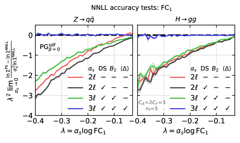
Figure 2: Test of NNLL accuracy of the PanGlobal (PG${}_{\beta=0}^{\text{sdf}}$) shower for the cumulative distribution of the Cambridge $y_{23}$ resolution variable, compared to known results for $Z\to q\bar{q}$ [52] (left) and $H\to gg$ [77] (right). The curves show the difference relative to NNLL for various subsets of ingredients. Starting from the red curve, DS additionally includes double soft contributions and $2$-jet NLO matching; $3\ell$ includes 3-loop running of $\alpha_{s}$ and the $K_{2}^{\text{resum}}$ term. Including all effects (blue line) gives a result that is consistent with zero, i.e. in agreement with NNLL.

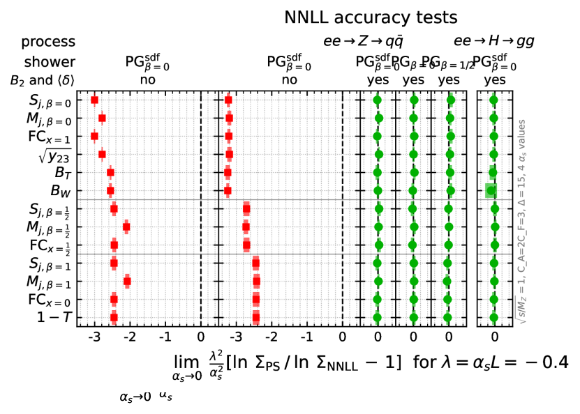
Figure 3: Summary of NNLL tests across observables and shower variants. Results consistent with zero (shown in green) are in agreement with NNLL. The observables correspond to the event shapes used in Ref. [5] and they are grouped according to the power ($\beta_{\text{obs}}$) of their dependence on the emission angle. All showers that include the corrections of this Letter agree with NNLL.

Tests across a wider range of observables and shower variants are shown in Fig. 3 for a fixed value of $\lambda=\alpha_{s}\ln v=-0.4$. With the drifts and all other contributions included, there is good agreement with the NNLL predictions [45, 46, 47, 48, 49, 50, 51, 52, 58, 61, 77].

Earlier work on NLL accuracy had found that the coefficients of NLL violations in common showers tended to be moderate for relatively inclusive observables like event shapes [5]. In contrast, here we see that non-NNLL showers differ from NNLL accuracy with coefficients of order one. That suggests a potential non-negligible phenomenological effect.

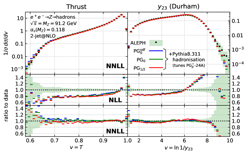
Figure 4: Results for the Thrust and Durham $y_{23}$ [78] observables with the PanGlobal showers compared to ALEPH data [79], using $\alpha_{s}(M_{Z})=0.118$. The lower (middle) panel shows the ratios of the NNLL (NLL) shower variants to data.

Fig. 4 compares three PanGlobal showers with ALEPH data [79] using Rivet v3 [80], illustrating the showers in their NLL and NNLL variants, with $\alpha_{s}^{\overline{\textsc{ms}}}(M_{Z})=0.118$ for both. We use $2$-jet NLO matching [74], and the NODS colour scheme [6], which guarantees full-colour accuracy in terms up to NLL for global event shapes. Our showers are implemented in a pre-release of PanScales [81] v0.2.0, interfaced to Pythia v8.311 [3] for hadronisation, with non-perturbative parameters tuned to ALEPH [82, 79] and L3 [83] data (starting from the Monash 13 tune [84], cf. Ref. [72] §.5; the tune has only a modest impact on the observables of Fig. 4). The impact of the NNLL terms is significant and brings the showers into good agreement with ALEPH data [79], both in terms of normalisation and shape. Some caution is required in interpreting the results: given that the logarithms are not particularly large at LEP energies, NLO 3-jet corrections (not included) may also play a significant role and should be studied in future work. Furthermore, the PanGlobal showers do not include finite quark-mass effects. Still, Fig. 4 suggests that NNLL terms have the potential to resolve a long-standing issue in which a number of dipole showers (including notably the Pythia 8 shower, but also the PanGlobal NLL shower) required an anomalously large value of $\alpha_{s}(m_{Z})\gtrsim 0.130$ [84] to achieve agreement with the data.

The parton showers developed here are expected to achieve NNLL (leading-colour) accuracy also for non-global event shapes such as hemisphere or jet observables, and $\alpha_{s}^{n}L^{n-1}$ (NSL) accuracy [54, 85, 62, 86, 63, 64, 68] for the soft-drop [87, 88] family of observables, in the limit where either their $z_{\text{cut}}$ parameter is taken small or $\beta_{\text{{sd}}}>0$. (We have not carried out corresponding logarithmic-accuracy tests, because the small $z_{\text{cut}}$ limit renders them somewhat more complicated than those of Figs. 2–3. In the case of non-global event shapes, there exist no reference calculations.) This is in addition to the NSL accuracy for energy-flow in a slice [89, 90, 91] and $\alpha_{s}^{n}L^{2n-2}$ (NNDL) accuracy for subjet multiplicities [92] that was already achieved with the inclusion of double-soft corrections [29].

Next objectives in the programme of bringing higher logarithmic accuracy to parton showers should include incorporation of full triple-collinear splitting functions (as relevant for experimentally important observables such as fragmentation functions), the extension to initial-state radiation, and logarithmically consistent higher-order matching for a variety of hadron-collider processes. The results presented here, a significant advance in their own right, also serve to give confidence in the feasibility and value of this broad endeavour.

oneΔ

Supplemental material

.1 Demonstration of relation between $\Delta K$ and drift

To help understand why Eq. (5) holds, we choose here to focus on the “non-Abelian” or “correlated-emission” channels, which for a quark emitter correspond to the terms involving $C_{F}n_{f}$ and $C_{F}C_{A}$ colour factors. In general, in the soft limit, we define the correlated contribution as being the part of the matrix element that remains after subtraction of the double independent-emission contribution, which in the case of a quark emitter corresponds to the $C_{F}^{2}$ component of the matrix element.

The starting point is a definition for $\Delta K_{1}(y_{\tilde{\imath}})$, to be understood with a renormalisation scale of $\mu=k_{t{\tilde{\imath}}}$,

$$K_{1}+\Delta K_{1}(y_{\tilde{\imath}})=\frac{1}{\mathcal{B}_{\tilde{\imath}}}\left(\mathcal{V}_{{\tilde{\imath}}}+\int d\Phi_{ij|{\tilde{\imath}}}^{\text{{ps}}}\,\mathcal{R}_{ij}\right).$$ (13)

It is convenient to define

$$R(y_{{\tilde{\imath}}},y_{d})=\frac{1}{\mathcal{B}_{\tilde{\imath}}}\left(\mathcal{V}_{{\tilde{\imath}}}\,\delta(y_{\tilde{\imath}}-y_{d})+\int d\Phi_{ij|{\tilde{\imath}}}^{\text{{ps}}}\,\mathcal{R}_{ij}\,\delta(y_{d}(i,j)-y_{d})\right),$$ (14)

where $y_{d}(i,j)$ denotes the effective rapidity of the $i,j$ descendants, as produced by the shower. In the correlated-emission channels, it is to be taken as the rapidity of $i+j$. The discussion can be adapted to the independent-emission channel by instead taking $y_{d}$ to be the rapidity of either $i$ or $j$, choosing the one with the larger shower ordering variable ($v_{\text{{ps}}}=k_{t}e^{-\beta_{\text{{ps}}}|y|}$).

It is useful to introduce a few properties of $R(y_{{\tilde{\imath}}},y_{d})$. Firstly, a trivial rewriting of Eq. (13) is that

$$K_{1}+\Delta K_{1}(y_{\tilde{\imath}})=\int_{-\infty}^{+\infty}dy_{d}\,R(y_{{\tilde{\imath}}},y_{d})\,.$$ (15)

For the integral to converge, $R(y_{{\tilde{\imath}}},y_{d})$ must vanish sufficiently fast when $|y_{d}-y_{\tilde{\imath}}|$ is large,

$$R(y_{{\tilde{\imath}}},y_{d})\to 0\,,\qquad\text{for }|y_{d}-y_{\tilde{\imath}}|\gg 1\,,$$ (16)

which can be seen as a consequence of the fact that for large rapidity separations between $i$ and $j$, the shower reduces to independent emission (cf. the PanScales conditions [5]). A second property of $R(y_{{\tilde{\imath}}},y_{d})$ is that

$$K_{1}=\int_{-\infty}^{+\infty}dy_{{\tilde{\imath}}}\,R(y_{{\tilde{\imath}}},y_{d})\,,$$ (17)

independently of $y_{d}$. This corresponds to the statement that if one integrates over $y_{{\tilde{\imath}}}$, the shower will generate the correct rate of soft-parton pairs for any $y_{d}$ — it is an essential property of a shower that has the correct double-soft contributions as in Ref. [29]. At large rapidities (but where the particles are still soft), $R(y_{{\tilde{\imath}}},y_{d})$ becomes a function of just $y_{d}-y_{{\tilde{\imath}}}$. Denoting that function as $\bar{R}$, we have

$$R(y_{{\tilde{\imath}}},y_{d}) \to\bar{R}(y_{d}-y_{\tilde{\imath}}),\qquad\text{for }y_{{\tilde{\imath}}},y_{d}\gg 1\,,$$ (18a)

$$R(y_{{\tilde{\imath}}},y_{d}) \to\bar{R}(y_{\tilde{\imath}}-y_{d}),\qquad\text{for }-y_{{\tilde{\imath}}},-y_{d}\gg 1\,.$$ (18b)

This then implies that $\Delta K_{1}(y_{\tilde{\imath}})$ tends to zero at large $|y_{\tilde{\imath}}|$, because Eqs. (15) and (17) become equivalent.

Now let us verify Eq. (5), which can be written as the large-$Y$ limit of

$$\Delta K_{1}^{\text{int}}(Y)=\int_{-Y}^{+Y}dy_{\tilde{\imath}}\,\Delta K_{1}(y_{\tilde{\imath}}) =\int_{-Y}^{+Y}dy_{\tilde{\imath}}\int_{-\infty}^{+\infty}dy_{d}\,R(y_{{\tilde{\imath}}},y_{d})-\int_{-Y}^{+Y}dy_{d}\int_{-\infty}^{+\infty}dy_{\tilde{\imath}}\,R(y_{{\tilde{\imath}}},y_{d})\,,$$ (19)

where, on the right-hand side, the last term is obtained by writing $2YK_{1}$ in terms of Eq. (17) for the factor of $K_{1}$ and an integral over $y_{d}$ for the factor $2Y$. Noting that the integration region where both rapidities are in the range $-Y$ to $Y$ cancels between the two terms, we get

$$\frac{1}{2}\Delta K_{1}^{\text{int}}(Y)=\int_{-Y}^{+Y}dy_{\tilde{\imath}}\int_{Y}^{+\infty}dy_{d}\,R(y_{{\tilde{\imath}}},y_{d})-\int_{-Y}^{+Y}dy_{d}\int_{Y}^{+\infty}dy_{\tilde{\imath}}\,R(y_{{\tilde{\imath}}},y_{d})\,,$$ (20)

where the factor of $1/2$ accounts for the fact that we consider just the positive infinite rapidity range (the negative infinite rapidity range gives identical results, notably since $R(y_{\tilde{\imath}},y_{d})=R(-y_{\tilde{\imath}},-y_{d})$). Next, we make use of the property that the integrand is dominated by a region where $y_{\tilde{\imath}}$ and $y_{d}$ are not too different (cf. Eq. (16)), change variables to $\Delta_{y}\equiv y_{d}-y_{\tilde{\imath}}$ and $\bar{y}=y_{\tilde{\imath}}-Y$, take the limit $Y\to\infty$ and use Eq. (18a) so as to write

$$\frac{1}{2}\Delta K_{1}^{\text{int}}\equiv\lim_{Y\to\infty}\frac{1}{2}\Delta K_{1}^{\text{int}}(Y)=\int_{0}^{+\infty}d\Delta_{y}\int_{-\Delta_{y}}^{0}d\bar{y}\,\bar{R}(\Delta_{y})-\int_{-\infty}^{0}d\Delta_{y}\int_{0}^{-\Delta_{y}}d\bar{y}\,\bar{R}(\Delta_{y})\,.$$ (21)

The $d\bar{y}$ integrations can be performed trivially and assembling both terms, we obtain

$$\frac{1}{2}\Delta K_{1}^{\text{int}}=\int_{-\infty}^{+\infty}d\Delta_{y}\Delta_{y}\,\bar{R}(\Delta_{y})=\lim_{{\tilde{\imath}}\to\text{{sc}}}\frac{1}{\mathcal{B}_{\tilde{\imath}}}\int d\Phi_{ij|{\tilde{\imath}}}^{\text{{ps}}}\,\mathcal{R}_{ij}\times(y_{d}-y_{\tilde{\imath}})\,,$$ (22)

which coincides with Eq. (5).

.2 Relation of $B_{2}$ coefficients with Refs. [67, 68]

.2.1 Overview of quark case

Refs. [67, 68] consider a collinear $q\to qg$ splitting probability, with original quark energy $E$, splitting opening angle $\theta$ and outgoing quark energy $\zeta E$. Eq. (2.10) of Ref. [68] defines the splitting probability as

$$\frac{\alpha_{s}(\mu)}{2\pi}\mathcal{P}_{q}(\zeta,\theta)\equiv\frac{\alpha_{s}(\mu)}{2\pi}\left\{\frac{2C_{F}}{1-\zeta}\!\left[1+\frac{\alpha_{s}(\mu)}{2\pi}\!\left(\!K_{1}+\beta_{0}\ln\frac{\mu^{2}}{(1-\zeta)^{2}E^{2}\theta^{2}}\right)\right]+\mathcal{B}_{1}^{q}(\zeta)+\frac{\alpha_{s}(\mu)}{2\pi}\!\left(\!\mathcal{B}_{2}^{q}(\zeta)+\mathcal{B}_{1}^{q}(\zeta)\beta_{0}\ln\frac{\mu^{2}}{E^{2}\theta^{2}}\right)\!\right\}\!,$$ (23)

where $\mathcal{B}_{1}^{q}(\zeta)=-C_{F}(1+\zeta)$ is the finite part of the $q\to qg$ splitting function and $\mathcal{B}_{2}^{q}(\zeta)$ is to be found in Refs. [67, 68]. Specifically, we will need the integral of $\mathcal{B}_{2}^{q}(\zeta)$, Eqs. (3.6), (3.4) and (3.7) of Ref. [68],

$$\int_{0}^{1}d\zeta\,\mathcal{B}_{2}^{q}(\zeta)=-\gamma_{q}^{(2)}+\beta_{0}X_{\theta^{2}}^{q}\,,$$ (24)

with

$$\gamma_{q}^{(2)}=C_{F}^{2}\left(\frac{3}{8}-\frac{\pi^{2}}{2}+6\zeta_{3}\right)+C_{F}C_{A}\left(\frac{17}{24}+\frac{11\pi^{2}}{18}-3\zeta_{3}\right)-C_{F}n_{f}T_{R}\left(\frac{1}{6}+\frac{2\pi^{2}}{9}\right),\qquad X_{\theta^{2}}^{q}=C_{F}\left(\frac{2\pi^{2}}{3}-\frac{13}{2}\right).$$ (25)

In that same collinear limit, up to order $\alpha_{s}^{2}$, let us write the parton shower’s splitting probability as

$$\frac{\alpha_{\text{eff}}}{2\pi}P_{gq}(z)=\frac{\alpha_{s}(k_{t})}{2\pi}P_{gq}(z)\left[1+\frac{\alpha_{s}(k_{t})}{2\pi}\left(K_{1}+B_{2}^{\text{{nlo}}}(z)+B_{2}^{\text{drift}}(z)\right)\right],$$ (26)

where we have separated $B_{2}(z)$ of Eq. (2) into two pieces. The piece $P_{gq}(z)B_{2}^{\text{{nlo}}}(z)$ will integrate to $2C_{F}B_{2}^{\text{int,\text{{nlo}}}}$, while $P_{gq}(z)B_{2}^{\text{drift}}(z)$ will integrate to $-2C_{F}\langle\Delta_{\ln z}\rangle$ in Eq. (6). The fundamental constraint that we will impose is that the integrals of Eqs. (23) and (26) should yield identical results provided that they cover equivalent phase space regions and include the full hard collinear domain.

Let us first examine the equivalence requirement if we consider limits just on the $1\to 2$ phase space, with $z\equiv 1-\zeta$ (the breaking of this equivalence at the level of the full $1\to 3$ phase space will be examined below and included through $B_{2}^{\text{drift}}(z)$). In doing so, it is important to identify the relation between $k_{t}$ in the shower and the kinematics of a hard collinear splitting. For the PanGlobal family of showers, it is straightforward to show that

$$k_{t}^{\text{PG}}\equiv zE\theta\,.$$ (27)

Setting $\mu=(1-\zeta)E\theta$ in Eq. (23), we can then write

$$\lim_{\epsilon\to 0}\int_{\epsilon}^{1-\epsilon}d\zeta\left[\frac{2C_{F}}{1-\zeta}K_{1}+\mathcal{B}_{2}^{q}(\zeta)+2\mathcal{B}_{1}^{q}(\zeta)\beta_{0}\ln(1-\zeta)\right]=\lim_{\epsilon\to 0}\int_{\epsilon}^{1-\epsilon}dzP_{gq}(z)(K_{1}+B_{2}^{\text{{nlo}}}(z))\,,$$ (28)

from which we deduce

$$2C_{F}B_{2}^{\text{int,NLO}}=\int_{0}^{1}dz\left(\mathcal{B}^{q}_{2}(1-z)+\mathcal{B}^{q}_{1}(1-z)\left[2\beta_{0}\ln z-K_{1}\right]\right)=-\gamma_{q}^{(2)}+C_{F}\beta_{0}\left(\frac{2\pi^{2}}{3}-3\right)+\frac{3}{2}C_{F}K_{1}\,.$$ (29)

Recall that the $z$ dependence that we assign to $B_{2}^{\text{{nlo}}}(z)$ is arbitrary for event-shape NNLL accuracy, as long as the integral in Eq. (3) converges, i.e. $B_{2}^{\text{{nlo}}}(z)$ has to vanish sufficiently fast as $z\to 0$. Our choice is

$$B_{2}^{\text{{nlo}}}(z)=\frac{3z}{2}B_{2}^{\text{int,NLO}}\,.$$ (30)

.2.2 Overview of gluon case

The case of $B_{2}^{\text{{nlo}}}(z)$ for gluon jets essentially follows the same steps as that in the quark case modulo a few subtleties that require extra care. For the sake of conciseness, we only discuss the main steps in the paragraphs below.

In the gluon case, the splitting probability is given by Eq. (7.2) of Ref. [68]. The $z\leftrightarrow 1-z$ symmetry of gluon splittings, also equivalent to the fact that parton showers generate gluon splitting by summing over two dipoles, can be used to recast this equation as

$$\frac{\alpha_{s}(k_{t})}{2\pi}\mathcal{P}_{g}(\zeta,\theta)\equiv\frac{\alpha_{s}(k_{t})}{2\pi}\left\{\frac{2C_{A}}{1-\zeta}\!\left(1+\frac{\alpha_{s}(k_{t})}{2\pi}K_{1}\right)+\mathcal{B}_{1}^{g}(\zeta)+\frac{\alpha_{s}(k_{t})}{2\pi}\left[\mathcal{B}_{2}^{g}(\zeta)+2\mathcal{B}_{1}^{g}(\zeta)\beta_{0}\ln(1-\zeta)\right]\right\},$$ (31)

with $\mu=k_{t}\equiv(1-\zeta)\theta E$. Here, we have explicitly summed the $g\to gg$ and $g\to q\bar{q}$ channels by introducing $\mathcal{B}_{1}^{g}=\mathcal{B}_{1}^{gg}+\mathcal{B}_{1}^{qg}=C_{A}(\zeta(1-\zeta)-2)+n_{f}T_{R}(\zeta^{2}+(1-\zeta)^{2})$ and $\mathcal{B}_{2}^{g}=\mathcal{B}_{2}^{gg}+\mathcal{B}_{2}^{qg}$ so that

$$\int_{0}^{1}d\zeta\,\mathcal{B}_{2}^{g}(\zeta)=-\gamma_{g}^{(2)}+\beta_{0}X_{\theta^{2}}^{g}\,,$$ (32)

with

$$\gamma_{g}^{(2)}=\left(\frac{8}{3}+3\zeta_{3}\right)C_{A}^{2}-\frac{4}{3}C_{A}n_{f}T_{R}-C_{F}n_{f}T_{R}\,,\qquad X_{\theta^{2}}^{g}=-\left(\frac{67}{9}-\frac{2\pi^{2}}{3}\right)C_{A}+\frac{23}{9}n_{f}T_{R}\,.$$ (33)

In writing this set of equations, we have performed a few simplifications. First, we have taken into account that, as in the quark case, the coupling for PanGlobal is evaluated at the scale $\mu=k_{t}\equiv k_{t}^{\text{PG}}=zE\theta$. Then, Eq. (32) differs from the corresponding equation (4.2) in Ref. [68] in that it does not include the $\mathcal{F}_{\text{clust.}}^{C_{A}^{2}}$ contribution. This contribution was an artefact of the use of an mMDT [87] procedure to define $z$ and $\theta$ in the $C_{A}^{2}$ channel, which does not apply in our case. We also refer to the discussion in Appendix E of Ref. [68] for more details.

With this in hand, the procedure follows exactly what we did above in the quark case, yielding

$$2C_{A}B_{2}^{\text{int,NLO}}=\int_{0}^{1}dz\left(\mathcal{B}_{2}^{g}(1-z)+\mathcal{B}_{1}^{g}(1-z)\left[2\beta_{0}\ln z-K_{1}\right]\right)=-\gamma_{g}^{(2)}+\left[\left(\frac{2\pi^{2}}{3}-\frac{67}{18}\right)C_{A}+\frac{10}{9}n_{f}T_{R}\right]\beta_{0}+\beta_{0}K_{1}\,.$$ (34)

This contribution has to be distributed over the two dipoles that contribute to the emission rate from a gluon. When implementing this in a shower, we also have the freedom to distribute this contribution over the $g\to gg$ and $g\to q\bar{q}$ channels as well as the freedom, already present in the quark case, to choose any explicit $z$ dependence as long as the gluon-splitting analogue of Eq. (3) is satisfied. In practice, we choose to have a unique $B_{2,g}^{\text{{nlo}}}(z)$ common to both splitting channels and take

$$B_{2,g}^{\text{{nlo}}}(z)=\frac{24C_{A}}{15C_{A}+2n_{f}T_{R}}z\,B_{2}^{\text{int,NLO}},$$ (35)

where the prefactor accompanies the shower-specific partitioning prescription for the splitting functions $P_{gg}(z)=C_{A}\frac{1+(1-z)^{3}}{2z}$ and $P_{qg}(z)=n_{f}T_{R}(1-z)^{2}$, for each of the two dipoles contributing to a given gluon. Note that, for event shapes, we are allowed to take a unique $B_{2,g}^{\text{{nlo}}}(z)$ across $g\to gg$ and $g\to q\bar{q}$ splittings since its contribution only appears in the Sudakov exponent where it is summed over flavour channels.

.2.3 Drift contributions

Concentrating once again on the correlated-emission channels, let us schematically write $B_{2}^{\text{{nlo}}}(z)$ as

$$K_{1}+B_{2}^{\text{{nlo}}}(z)\equiv\frac{1}{\mathcal{B}_{{\tilde{\imath}}{\tilde{k}}}}\left(\mathcal{V}_{{\tilde{\imath}}{\tilde{k}}}+\int d\Phi_{ijk|{\tilde{\imath}}{\tilde{k}}}^{\text{{nlo}}}\,\mathcal{R}_{ijk}\right),$$ (36)

where in the quark branching channel ${\tilde{\imath}}$ is a gluon, ${\tilde{k}}$ is a quark, $z=E_{\tilde{\imath}}/(E_{\tilde{\imath}}+E_{\tilde{k}})$ and we assume the same scale choice $\mu=zE\theta$ as above. This is the extension of Eq. (13) to the collinear region noting that (a) in the soft-collinear region, $\Delta K_{1}(y)$ and $B_{2}(z)$ both go to zero and (b) the “Born” starting point is a collinear ${\tilde{\imath}}{\tilde{k}}$ splitting, rather than just a soft ${\tilde{\imath}}$ emission. In the correlated-emission channels, the $d\Phi_{ijk|{\tilde{\imath}}{\tilde{k}}}^{\text{{nlo}}}$ phase space map is organised such that the energy fraction carried by the $ij$ pair is equal to that carried by ${\tilde{\imath}}$, $E_{i}+E_{j}=E_{\tilde{\imath}}$, where ${\tilde{\imath}}$ is the emitted gluon (the calculation also preserves $\theta_{ij,k}=\theta_{{\tilde{\imath}}{\tilde{k}}}$).

Let us now suppose that we had a parton shower with tree-level $1\to 3$ splittings and 1-loop $1\to 2$ splittings. That shower would implicitly involve a $B_{2}^{\text{{ps}}}(z)$. In what follows, we will work out the relation between the integral of $B_{2}^{\text{{ps}}}(z)$ and that of $B_{2}^{\text{{nlo}}}(z)$ and observe that this difference depends only on the behaviour of the shower in the soft collinear region, where the triple-collinear structure reduces to the double-soft structure. This will be useful, because event-shape NNLL accuracy will be sensitive just to the integral of $B_{2}(z)$, through its impact on the Sudakov form factor. Thus, even if our actual shower does not have the full triple-collinear structure, the integral of $B_{2}^{\text{{ps}}}(z)$ that we determine for an imaginary shower that does have that structure will be sufficient to achieve NNLL event-shape accuracy in the actual shower.

The $B_{2}^{\text{{ps}}}(z)$ function can be expressed as

$$K_{1}+B_{2}^{\text{{ps}}}(z)\equiv\frac{1}{\mathcal{B}_{{\tilde{\imath}}{\tilde{k}}}}\left(\mathcal{V}_{{\tilde{\imath}}{\tilde{k}}}+\int d\Phi_{ijk|{\tilde{\imath}}{\tilde{k}}}^{\text{{ps}}}\,\mathcal{R}_{ijk}\right),$$ (37)

where $d\Phi_{ijk|{\tilde{\imath}}{\tilde{k}}}^{\text{{ps}}}$ reflects the parton-shower kinematic map and associated partitioning of phase space. In particular the shower map will not in general have $E_{i}+E_{j}=E_{\tilde{\imath}}$ or $\theta_{ij,k}=\theta_{{\tilde{\imath}}{\tilde{k}}}$. Next, defining $B_{2}^{\text{drift}}=B_{2}^{\text{{ps}}}(z)-B_{2}^{\text{{nlo}}}(z)$ so as to obtain Eq. (26), we have

$$2C_{F}B_{2}^{\text{int,drift}}\equiv\int_{0}^{1}dzP_{gq}(z)B_{2}^{\text{drift}}(z)=\lim_{\epsilon\to 0}\int_{\epsilon}^{1}dz\,P_{gq}(z)\left[B_{2}^{\text{{ps}}}(z)-B_{2}^{\text{{nlo}}}(z)\right].$$ (38)

It is now convenient to introduce a representation of the integrand of Eq. (36) that is differential in the energy fraction $z_{d}$ of the descendants (e.g. $z_{d}=z_{i}+z_{j}$ in the non-Abelian channel)

$$K_{1}+B_{2}^{\text{{nlo}}}(z)=\int dz_{d}R^{\text{{nlo}}}(z,z_{d})\,,\qquad R^{\text{{nlo}}}(z_{\tilde{\imath}},z_{d})=\frac{1}{\mathcal{B}_{{\tilde{\imath}}{\tilde{k}}}}\left(\mathcal{V}_{{\tilde{\imath}}{\tilde{k}}}\delta(z_{d}-z_{\tilde{\imath}})+\int d\Phi_{ijk|{\tilde{\imath}}{\tilde{k}}}^{\text{{nlo}}}\,\mathcal{R}_{ijk}\delta(z_{d}-z_{d}(i,j))\right)\,.$$ (39)

For the NLO phase-space map discussed above $R^{\text{{nlo}}}(z,z_{d})$ is equal to $(K_{1}+B_{2}^{\text{{nlo}}}(z))\delta(z-z_{d})$. One can also define an analogue for the parton shower, $R^{\text{{ps}}}(z,z_{d})$, which will have a more complex structure. We can rewrite Eq. (38) as

$$2C_{F}B_{2}^{\text{int,drift}}=\lim_{\epsilon\to 0}\int_{0}^{1}dz_{d}\int_{0}^{1}dzP_{gq}(z)\left[R^{\text{{ps}}}(z,z_{d})-R^{\text{{nlo}}}(z,z_{d})\right]\Theta(z-\epsilon)\,.$$ (40)

Within our assumption that the shower has the correct triple collinear (and double-collinear virtual) content, the total amount of radiation at a given $z_{d}$ will be reproduced by the parton shower, i.e.

$$\int_{0}^{1}dzP_{gq}(z)R^{\text{{ps}}}(z,z_{d})=\int_{0}^{1}dzP_{gq}(z)R^{\text{{nlo}}}(z,z_{d})\,.$$ (41)

Furthermore, as in the case of section .1, any sensible shower that satisfies the PanScales conditions will have the property that the integral over $R^{\text{{ps}}}(z,z_{d})$ is dominated by the region of $z\sim z_{d}$. For finite $z_{d}$, the $\Theta(z-\epsilon)$ term in Eq. (40) is irrelevant. Therefore if we place an upper limit on the $z_{d}$ integral, $z_{d}\ll\epsilon_{d}$, with $\epsilon\ll\epsilon_{d}\ll 1$, the result will be unchanged,

$$2C_{F}B_{2}^{\text{int,drift}}=\lim_{\begin{subarray}{c}\epsilon_{d}\to 0\\ \epsilon/\epsilon_{d}\to 0\end{subarray}}\int_{0}^{\epsilon_{d}}dz_{d}\int_{0}^{1}dzP_{gq}(z)\left[R^{\text{{ps}}}(z,z_{d})-R^{\text{{nlo}}}(z,z_{d})\right]\Theta(z-\epsilon)\,.$$ (42)

Given that the integral now just involves a region of small $z$ and $z_{d}$, i.e. we are in the soft-collinear limit, we can use the property that aside from an overall $1/z_{d}$ factor, $R^{\text{{ps}}}(z,z_{d})$ is a function just of the ratio of $z_{d}/z$

$$R^{\text{{ps}}}(z,z_{d}) \overset{z,z_{d}\ll 1}{\longrightarrow}\frac{1}{z_{d}}\bar{R}^{\text{{ps}}}(z_{d}/z)\,,$$ (43a)

$$R^{\text{{nlo}}}(z,z_{d}) \overset{z,z_{d}\ll 1}{\longrightarrow}\frac{K_{1}}{z_{d}}\delta(z_{d}/z-1)\,.$$ (43b)

In this limit, we can also use the soft limit of $P_{gq}(z)$ as $z\sim z_{d}\ll 1$, allowing us to write

$$2C_{F}B_{2}^{\text{int,drift}} =2C_{F}\lim_{\begin{subarray}{c}\epsilon_{d}\to 0\\ \epsilon/\epsilon_{d}\to 0\end{subarray}}\int_{0}^{\epsilon_{d}}\frac{dz_{d}}{z_{d}}\int_{0}^{1}\frac{dz}{z}\left[\bar{R}^{\text{{ps}}}(z_{d}/z)-K_{1}\delta(z_{d}/z-1)\right]\Theta(z-\epsilon)$$ (44a)

$$=2C_{F}\lim_{\begin{subarray}{c}\epsilon_{d}\to 0\\ \epsilon/\epsilon_{d}\to 0\end{subarray}}\int_{0}^{\infty}\frac{d\xi}{\xi}\ln\frac{\epsilon_{d}}{\xi\epsilon}\left[\bar{R}^{\text{{ps}}}(\xi)-K_{1}\delta(\xi-1)\right]\,.$$ (44b)

To get the second line, we have replaced $z\to z_{d}/\xi$, used the fact that $R^{\text{{ps}}}(\xi)$ vanishes for $\xi\to 0$ to replace the lower limit of the $\xi$ integrand with $0$, and exchanged the order of $z_{d}$ and $\xi$ integrations.

Next, exploiting the fact that $\int_{0}^{\infty}d\xi/\xi\bar{R}^{\text{{ps}}}(\xi)=K_{1}$, we can see that the $\ln\epsilon_{d}/\epsilon$ contribution vanishes, leaving

$$2C_{F}B_{2}^{\text{int,drift}}=2C_{F}\int_{0}^{\infty}\frac{d\xi}{\xi}\ln\frac{1}{\xi}\,\bar{R}^{\text{{ps}}}(\xi)\equiv-2C_{F}\langle\Delta_{\ln z}\rangle\,,$$ (45)

which is the basis for Eq. (6).

Eq. (7) expresses the $\langle\Delta_{\ln z}\rangle$ in terms of $\langle\Delta_{y}\rangle$ and $\langle\Delta_{\ln m_{t}}\rangle$. The relation between $\langle\Delta_{\ln m_{t}}\rangle$ and $\langle\Delta_{\ln k_{t}}\rangle$ is given by

$$\langle\Delta_{\ln m_{t}}\rangle-\langle\Delta_{\ln k_{t}}\rangle=\int d\Phi^{\text{{ps}}}_{ij|{\tilde{\imath}}}\,\mathcal{R}(i,j)\,\frac{1}{2}\ln\frac{m_{t,ij}^{2}}{k_{t,ij}^{2}}\,.$$ (46)

Note that aside from the phase space map, the integrand does not depend on ${\tilde{\imath}}$. Accordingly, as long as the phase space map covers the full double-soft region, which it does for any soft collinear ${\tilde{\imath}}$, we are free to replace the parton-shower phase space map with an analytic one that preserves $k_{t}$ and rapidity. One can then deduce the result for Eq. (46) from the corresponding expressions in the literature, e.g. Eqs. (3.7)–(3.12) of Ref. [58],

$$\langle\Delta_{\ln m_{t}}\rangle-\langle\Delta_{\ln k_{t}}\rangle=-\beta_{0}\frac{\pi^{2}}{12}\,.$$ (47)

We have also verified this numerically for each of our shower maps.

.3 Multiple emission contribution

In our definition, the function $\mathcal{F}$ in Eq. (1) accounts for the difference between applying a separate condition $\Theta(V(k_{\tilde{\imath}})<v)$ on each primary emission ${\tilde{\imath}}$, versus applying a single condition $\Theta(V(\{k_{i}\})<v)$ on the full set of emissions after branching. It starts at order $\alpha_{s}^{2}$ and its NNLL component (starting from $\alpha_{s}^{2}L$) differs from the corresponding $\delta\mathcal{F}$ contribution which appears at NNLL accuracy in ARES [58], in that the latter also includes certain order $\alpha_{s}$ terms (cf. Eq. (2.45) of Ref. [58]). Let us start by defining a primary inclusive emission density

$$d\rho_{k}=2\frac{dk_{t}}{k_{t}}\,dzP_{gq}(z)\,\frac{\alpha_{\text{eff}}}{2\pi}\Theta(z>k_{t})\,,$$ (48)

which allows us to write the Sudakov factor from Eq. (1) as

$$S(v)=\exp\left[-2\int d\rho_{k}\,M(k)\Theta(V(k)>v)\right].$$ (49)

The factor of two in the Sudakov reflects the presence of two hemispheres. The matching factor $M(k)$ will be irrelevant in the remainder of this section because it tends to $1$ for $k_{t}\to 0$, but we will need it later in section .4. Up to NLL, one way of writing $\mathcal{F}$ is as

$$\mathcal{F}_{\text{{nll}}}=\frac{S(\epsilon v)}{S(v)}\sum_{n=0}^{\infty}\frac{1}{n!}\prod_{{\tilde{\imath}}=1}^{n}\left[2\int d\rho_{k_{\tilde{\imath}}}\,\Theta(V(k_{\tilde{\imath}})>\epsilon v)\right]\Theta(V(k_{\tilde{1}},\ldots,k_{\tilde{n}})<v),$$ (50)

where $S(\epsilon v)$ exponentiates the virtual corrections for no emission down to scale $\epsilon v$, the denominator $S(v)$ simply divides out the Sudakov factor already included in Eq. (1), while the sum and product account for the real emission of any number $n$ of primary particles ${\tilde{\imath}}$ at scales above $\epsilon v$. The final $\Theta$-function represents the constraint on the emissions from the requirement for the event-shape observable to have a value less than $v$. The parameter $\epsilon$ is to be taken small, such that $\ln\epsilon$ is kept finite or, equivalently, $v\ll\epsilon\ll 1$, so that one does not need to resum $\ln\epsilon$-enhanced terms, for example in the ratio $S(\epsilon v)/S(v)$.

Now let us extend Eq. (50) to NNLL. In the various manipulations along the way, we will discard contributions that are beyond NNLL (i.e. that are $\alpha_{s}^{n}L^{n-2}$ or higher). We start by writing

$$\mathcal{F}_{\text{{nnll}}}=\frac{S(\epsilon v)}{S(v)}\sum_{n=0}^{\infty}\bigg{\{}\frac{1}{n!}\prod_{{\tilde{\imath}}=1}^{n}\left[2\int d\rho_{k_{\tilde{\imath}}}\left(u_{\tilde{\imath}}+\frac{\alpha_{s}}{2\pi}\int d\Phi_{i_{a}i_{b}|{\tilde{\imath}}}\,\frac{\mathcal{R}_{i_{a}i_{b}}}{\mathcal{B}_{{\tilde{\imath}}}}\left[u_{i_{a}}u_{i_{b}}-u_{\tilde{\imath}}\right]\right)\Theta(V(k_{\tilde{\imath}})>\epsilon v)\right]\times\\ \times\Theta(V(\{k_{1}\},\{k_{2}\}\ldots,\{k_{n}\})<v)\bigg{\}},$$ (51)

where the $u_{\tilde{\imath}}$ notation, inspired by generating-functionals, means that in the second line, $\{k_{i}\}$ is just $k_{\tilde{\imath}}$, while $u_{i_{a}}u_{i_{b}}$ means that $\{k_{i}\}$ is to be understood as $k_{i_{a}},k_{i_{b}}$, i.e.

$$u_{{\tilde{\imath}}}\Theta(V(\left\{k_{1}\right\},\dots,\left\{k_{i}\right\},\dots,\left\{k_{n}\right\})<v) \equiv\Theta(V(\left\{k_{1}\right\},\dots,k_{\tilde{\imath}},\dots,\left\{k_{n}\right\})<v)\,,$$ (52a)

$$\quad u_{i_{a}}u_{i_{b}}\Theta(V(\left\{k_{1}\right\},\dots,\left\{k_{i}\right\},\dots,\left\{k_{n}\right\})<v) \equiv\Theta(V(\left\{k_{1}\right\},\dots,k_{i_{a}},k_{i_{b}},\dots,\left\{k_{n}\right\})<v)\,.$$ (52b)

Note that the ${\tilde{\imath}}\to i_{a}i_{b}$ branching is unitary in the soft-collinear region that dominates $\mathcal{F}$. The individual emission constraint $\Theta(V(k_{\tilde{\imath}})>\epsilon v)$ preserves this unitarity, and so one should similarly constrain just $V(k)>\epsilon v$ in the definition of $S(\epsilon v)$ of Eq. (51).

Next, we take advantage of freedom in how to define the unresolved emissions (e.g. $V(k_{\tilde{\imath}})<\epsilon v$), as long as we use consistent definitions of unresolved in the Sudakov and real emission contributions. In particular, we choose to place the resolution condition on final ($i_{a},i_{b}$) particles rather than the (potentially) intermediate ${\tilde{\imath}}$ particle, which gives

$$\mathcal{F}_{\text{{nnll}}}=\frac{\bar{S}(\epsilon v)}{S(v)}\sum_{n=0}^{\infty}\bigg{\{}\frac{1}{n!}\prod_{{\tilde{\imath}}=1}^{n}\left[2\int d\rho_{k_{\tilde{\imath}}}\left(u_{\tilde{\imath}}+\frac{\alpha_{s}}{2\pi}\int d\Phi_{i_{a}i_{b}|{\tilde{\imath}}}\,\frac{\mathcal{R}_{i_{a}i_{b}}}{\mathcal{B}_{{\tilde{\imath}}}}\left[u_{i_{a}}u_{i_{b}}-u_{\tilde{\imath}}\right]\right)\Theta(V(k_{i_{ab}})>\epsilon v)\right]\times\\ \times\Theta(V(\{k_{1}\},\{k_{2}\}\ldots,\{k_{n}\})<v)\bigg{\}}.$$ (53)

Relative to Eq. (51) there are two changes. Firstly, at the end of the square bracket on the first line, $\Theta(V(k_{{\tilde{\imath}}})>\epsilon v)$ has been replaced by $\Theta(V(k_{i_{ab}})>\epsilon v)$, where $k_{i_{ab}}$ is defined to be $k_{\tilde{\imath}}$ for the $u_{\tilde{\imath}}$ contribution, while for the $u_{i_{a}}u_{i_{b}}$ contribution it is equal to a massless momentum with the same transverse components and rapidity as $k_{i_{a}}+k_{i_{b}}$. The shower and resummation have different maps from ${\tilde{\imath}}$ to $i_{a}i_{b}$. However, both maps have the property that if one integrates over all possible ${\tilde{\imath}}$, one obtains identical final distributions of $i_{a}i_{b}$. Since the $\Theta(V(k_{i_{ab}})>\epsilon v)$ condition is a constraint on those final momenta, not on the (sometimes) intermediate ${\tilde{\imath}}$ momenta, the sum and product in Eq. (53) will be the same in the shower and in the resummation (at least up to NNLL). The second change to note in Eq. (53) relative to Eq. (51) is that $S(\epsilon v)$ has been substituted with $\bar{S}(\epsilon v)$, defined as

$$\bar{S}(\epsilon v)=\exp\left[-2\int d\rho_{k}\left(\Theta(V(k)>\epsilon v)+\frac{\alpha_{s}}{2\pi}\int d\Phi_{ab|k}\,\frac{\mathcal{R}_{ab}}{\mathcal{B}_{k}}\left[\Theta(V(k_{ab})>\epsilon v)-\Theta(V(k)>\epsilon v)\right]\right)\right].$$ (54)

As compared to the $S(\epsilon v)$ of Eq. (49), the $\Theta(V(k)>\epsilon v)$ factor has been replaced by conditions that are specified in terms of final momenta, either $k$ when there was no secondary branching or $k_{ab}$ when there was a branching (with $k_{ab}$ defined in analogy to $k_{i_{ab}}$ above). This modification is necessary in order for the exponentiated virtual corrections in $\bar{S}(\epsilon v)$ to exactly match the phase space in the real sum and product of Eq. (53), as required by unitarity.

Since the sum-product contribution in Eq. (53) is the same between the parton shower and the resummation, it will cancel in the ratio $\mathcal{F}^{\text{{ps}}}/\mathcal{F}^{\text{resum}}$, leaving us with

$$\frac{\mathcal{F}^{\text{{ps}}}}{\mathcal{F}^{\text{resum}}}=\frac{\bar{S}^{\text{{ps}}}(\epsilon v)}{\bar{S}^{\text{resum}}(\epsilon v)} =\exp\left[-2\int d\rho_{k}\left(\frac{\alpha_{s}}{2\pi}\int d\Phi_{ab|k}^{\text{{ps}}}\,\frac{\mathcal{R}_{ab}}{\mathcal{B}_{k}}[\Theta(V(k_{ab})>\epsilon v)-\Theta(V(k)>\epsilon v)]\right)\right].$$ (55)

To reach that result, it is useful to note that in $\bar{S}^{\text{resum}}$, the map $d\Phi_{ab|k}^{\text{resum}}$ has the property that $V(k_{ab})$ and $V(k)$ are identical, giving $\bar{S}^{\text{resum}}(\epsilon v)=S(\epsilon v)$. Our next step is to write $d\rho_{k}$ explicitly in the soft-collinear limit as $4C_{F}dk_{t}/k_{t}dy\alpha_{s}(k_{t})/2\pi$ and to use $V(k)\propto k_{t}\exp[-\beta_{\text{obs}}y]$. We then perform the $k_{t}$ integration within the limits set by the difference of $\Theta$-functions in Eq. (55). In doing so, it is convenient to approximate the scale of the coupling as $k_{t}\sim ve^{\beta_{\text{obs}}y}$, which is legitimate up to and including NNLL when focusing on the ratio of $\mathcal{F}^{\text{{ps}}}/\mathcal{F}^{\text{resum}}$. We then have

$$\frac{\mathcal{F}^{\text{{ps}}}}{\mathcal{F}^{\text{resum}}} =\exp\left[-8C_{F}\int_{0}^{\ln 1/v_{\text{hc}}}\!\!\!\!dy\int\frac{dk_{t}}{k_{t}}\delta\!\left(\ln\frac{k_{t}}{ve^{\beta_{\text{obs}}y}}\right)\frac{\alpha_{s}^{2}(k_{t})}{(2\pi)^{2}}\int d\Phi_{ab|k}^{\text{{ps}}}\,\frac{\mathcal{R}_{ab}}{\mathcal{B}_{k}}\left(\ln\frac{k_{t,ab}}{k_{t}}-\beta_{\text{obs}}(y_{ab}-y)\right)\right]$$ (56a)

$$=1-\frac{8C_{F}}{\beta_{\text{obs}}}T_{2}(v,v_{\text{hc}})\left[\langle\Delta_{\ln k_{t}}\rangle-\beta_{\text{obs}}\langle\Delta_{y}\rangle\right],$$ (56b)

where we have ignored any $\epsilon$ dependence (since we ignore $\ln\epsilon$ contributions) and in the second line we have transformed the $dy$ integral into a $1/\beta_{\text{obs}}dk_{t}/k_{t}$ integral so as to obtain the $T_{2}(v,v_{\text{hc}})$ function. The final result corresponds to Eq. (11). Note that for $\beta_{\text{obs}}=0$, the result is to be understood as the $\beta_{\text{obs}}\to 0$ limit of Eq. (56b), with $1/\beta_{\text{obs}}T_{2}(v,v_{\text{hc}})\to(\frac{\alpha_{s}(v)}{2\pi})^{2}\ln 1/v$.

.4 Equivalence with NNLL resummation

.4.1 Relation to the ARES approach

In the previous sections, we have given analytic arguments showing (i) how we can incorporate into the shower the hard-collinear $\mathcal{B}_{2}(z)$ computed analytically in Refs. [67, 68], (ii) how the various drift contributions emerge in the parton shower Sudakov and ultimately compensate for the effects of the shower’s double-soft map close to the observable boundary, cf. Eq. (12). In this section, we show that these ingredients, together with 3-loop running coupling, the CMW scheme ($K_{1}$ and $K_{2}$) and full double-soft matrix-element corrections are sufficient for the shower to achieve NNLL accuracy, for which we take ARES [58] as our reference.

Our starting point is the shower result, Eq. (1). Since the $\langle\Delta_{\ln k_{t}}\rangle$ and $\langle\Delta_{y}\rangle$ contributions all cancel, cf. Eq. (12) and sections .1, .2.3 and .3, we will leave them out in the rest of this section, or equivalently work as if they were zero. We then write Eq. (1) using the shorthand Eq. (49)

$$\Sigma^{\textsc{ps}}_{\textsc{nnll}}(v)=\mathcal{F}^{\textsc{ps}}_{\textsc{nnll}}(v)\,S^{\textsc{ps}}(v)\,.$$ (57)

It is useful to write the Sudakov form factor $S^{\text{{ps}}}$ separated into terms of different logarithmic order

$$\ln S^{\text{{ps}}}=(\ln S)_{\text{{ll}}}+(\ln S)_{\text{{nll}}}+(\ln S)_{\text{{nnll}}}+\ldots$$ (58)

We can write the individual orders as integrals either over $k_{t}$ and $z$ (as in Eq. (1) and in typical resummations), or as an integral over the shower ordering variable $v_{\text{{ps}}}$ and $z$. The latter gives slightly more complicated expressions, but helps connect with the actual shower algorithm. On a first pass, readers may wish to set $\beta_{\text{{ps}}}=0$, in which case $v_{\text{{ps}}}\equiv k_{t}$. One can also check explicitly that any dependence on $\beta_{\text{{ps}}}$ cancels separately at each logarithmic order. We take an observable that in the soft or collinear limit behaves as $V(k)=f(z)g(y)k_{t}e^{-\beta_{\text{obs}}y}$ with $f(z)\to 1$ for $z\to 0$ and $g(y)\to 1$ for $y\to\infty$. Using $z=k_{t}e^{y}$, we can write

$$k_{t}=z^{\frac{\beta_{\text{{ps}}}}{1+\beta_{\text{{ps}}}}}v_{\textsc{ps}}^{\frac{1}{1+\beta_{\text{{ps}}}}},\qquad V(k)=f(z)\,g(y)\,V_{\text{sc}}(k)\,,\quad\text{ with }\quad V_{\text{sc}}(k)=z^{\frac{\beta_{\text{{ps}}}-\beta_{\text{obs}}}{1+\beta_{\text{{ps}}}}}v_{\text{{ps}}}^{\frac{1+\beta_{\text{obs}}}{1+\beta_{\text{{ps}}}}}\,.$$ (59)

At LL, $P_{gq}(z)$ can be approximated as $2C_{F}/z$, the 3-jet matrix-element correction factor $M(k)$ can be ignored, and the observable can be approximated by its soft-collinear limit, yielding

$$(\ln S)_{\text{{ll}}}\equiv-\frac{4}{1+\beta_{\text{{ps}}}}\int_{0}^{1}\frac{dv_{\text{{ps}}}}{v_{\text{{ps}}}}\int_{v_{\text{{ps}}}}^{1}dz\frac{\alpha_{s}(z^{\frac{\beta_{\text{{ps}}}}{1+\beta_{\text{{ps}}}}}v_{\text{{ps}}}^{\frac{1}{1+\beta_{\text{{ps}}}}})}{2\pi}\frac{2C_{F}}{z}\,\Theta(z^{\frac{\beta_{\text{{ps}}}-\beta_{\text{obs}}}{1+\beta_{\text{{ps}}}}}v_{\text{{ps}}}^{\frac{1+\beta_{\text{obs}}}{1+\beta_{\text{{ps}}}}}>v)\,.$$ (60)

Note that we choose to include $3$-loop running for the coupling even in the LL contribution. Strictly speaking, this introduces subleading contributions in $(\ln S)_{\text{{ll}}}$, but it simplifies the expressions for the higher-order contributions, without compromising any of the arguments of this section. At NLL, we have

$$(\ln S)_{\text{{nll}}}\equiv -\frac{4K_{1}}{1+\beta_{\text{{ps}}}}\int_{0}^{1}\frac{dv_{\text{{ps}}}}{v_{\text{{ps}}}}\int_{v_{\text{{ps}}}}^{1}dz\frac{\alpha_{s}^{2}(z^{\frac{\beta_{\text{{ps}}}}{1+\beta_{\text{{ps}}}}}v_{\text{{ps}}}^{\frac{1}{1+\beta_{\text{{ps}}}}})}{(2\pi)^{2}}\frac{2C_{F}}{z}\,\Theta(z^{\frac{\beta_{\text{{ps}}}-\beta_{\text{obs}}}{1+\beta_{\text{{ps}}}}}v_{\text{{ps}}}^{\frac{1+\beta_{\text{obs}}}{1+\beta_{\text{{ps}}}}}>v)$$

$$-\frac{4B_{1}}{1+\beta_{\text{{ps}}}}\int_{0}^{1}\frac{dv_{\textsc{ps}}}{v_{\textsc{ps}}}\frac{\alpha_{s}(v_{\textsc{ps}}^{\frac{1}{1+\beta_{\text{{ps}}}}})}{2\pi}\,\Theta(v_{\textsc{ps}}^{\frac{1+\beta_{\text{obs}}}{1+\beta_{\text{{ps}}}}}>v),$$ (61)

where we have included the $K_{1}$ NLL contribution and introduced $B_{1}=\int_{0}^{1}dz\mathcal{B}_{1}(1-z)$. In the second line, we have substituted $z=1$ in the argument of $\alpha_{s}$ and the observable so as to have purely $\alpha_{s}^{n}L^{n}$ terms (aside from the higher-loop running coupling contributions). The independence of $(\ln S)_{\text{{ll}}}$ and $(\ln S)_{\text{{nll}}}$ of $\beta_{\text{{ps}}}$ can be verified, e.g. by changing variables from $v_{\text{{ps}}}$ to $v_{\text{obs}}\equiv V_{\text{sc}}(k)$.

The NNLL contributions can be written as

$$(\ln S)_{\text{{nnll}}}\equiv -\frac{4K_{2}^{\text{resum}}}{1+\beta_{\text{{ps}}}}\int_{0}^{1}\frac{dv_{\text{{ps}}}}{v_{\text{{ps}}}}\int_{v_{\text{{ps}}}}^{1}dz\frac{\alpha_{s}^{3}(z^{\frac{\beta_{\text{{ps}}}}{1+\beta_{\text{{ps}}}}}v_{\text{{ps}}}^{\frac{1}{1+\beta_{\text{{ps}}}}})}{(2\pi)^{3}}\frac{2C_{F}}{z}\,\Theta(z^{\frac{\beta_{\text{{ps}}}-\beta_{\text{obs}}}{1+\beta_{\text{{ps}}}}}v_{\text{{ps}}}^{\frac{1+\beta_{\text{obs}}}{1+\beta_{\text{{ps}}}}}>v)$$

$$-\frac{4\tilde{B}_{2}^{\text{{ps}}}}{1+\beta_{\text{{ps}}}}\int_{0}^{1}\frac{dv_{\textsc{ps}}}{v_{\textsc{ps}}}\frac{\alpha_{s}^{2}(v_{\textsc{ps}}^{\frac{1}{1+\beta_{\text{{ps}}}}})}{(2\pi)^{2}}\,\Theta(v_{\textsc{ps}}^{\frac{1+\beta_{\text{obs}}}{1+\beta_{\text{{ps}}}}}>v)+H_{1}^{\text{{ps}}}\frac{\alpha_{s}(Q)}{2\pi}+2C_{1,\text{hc}}^{\text{{ps}}}\frac{\alpha_{s}(v^{\frac{1}{1+\beta_{\text{obs}}}})}{2\pi}+C_{1,\text{wa}}^{\text{{ps}}}\frac{\alpha_{s}(v)}{2\pi}\,.$$ (62)

The $K_{2}^{\text{resum}}$ coefficient has already been introduced, and we elaborate on the others below. Note that each of the integrals is independent of $\beta_{\text{{ps}}}$, but some of the coefficients multiplying them depend on $\beta_{\text{{ps}}}$. Below, we will verify that this $\beta_{\text{{ps}}}$ dependence disappears when summing over all contributions.

Let us start with $H_{1}^{\text{{ps}}}$, which involves the $3$-jet matrix element correction factor $M(k)$,

$$H_{1}^{\text{{ps}}} =\lim_{\epsilon\to 0}\left[\frac{4}{1+\beta_{\text{{ps}}}}\int_{\epsilon}^{1}\frac{dv_{\text{{ps}}}}{v_{\text{{ps}}}}\int_{v_{\text{{ps}}}}^{1}dzP_{gq}(z)M(k)-\frac{4}{1+\beta_{\text{{ps}}}}\int_{\epsilon}^{1}\frac{dv_{\text{{ps}}}}{v_{\text{{ps}}}}\int_{v_{\text{{ps}}}}^{1}dzP_{gq}(z)\right]$$ (63a)

$$=\frac{4}{1+\beta_{\text{{ps}}}}\int_{0}^{1}\frac{dv_{\text{{ps}}}}{v_{\text{{ps}}}}\int_{v_{\text{{ps}}}}^{1}dzP_{gq}(z)\left(M(k)-1\right)\,.$$ (63b)

Note that $M(k)$ also accounts for the Jacobian associated with the integration variables and exact phase space limits. In the second line, the lower limit of the integration on $v_{\text{{ps}}}$ could be taken to zero, since $M(k)\to 1$ when $k_{t}\to 0$. Through unitarity, the shower is such that $\Sigma(v)$ is normalised to one, i.e. $\Sigma(v=1)=1$, which ensures that $H_{1}^{\text{{ps}}}$ can be determined fully from the real $3$-jet matrix element. The result is independent of the choice of observable,

$$H_{1}^{\text{{ps}}}=\frac{-C_{F}}{1+\beta_{\text{{ps}}}}\left(\frac{\pi^{2}}{3}(1+\beta_{\text{{ps}}})+\frac{7}{2}(1-\beta_{\text{{ps}}})\right).$$ (64)

Next we examine $C_{1,\text{hc}}^{\text{{ps}}}$,

$$C_{1,\text{hc}}^{\text{{ps}}} =\frac{-2}{1+\beta_{\text{obs}}}\int_{0}^{1}dzP_{gq}(z)\log f(z)-\frac{2}{1+\beta_{\text{obs}}}\int_{0}^{1}dz\mathcal{B}_{1}(1-z)\left(\frac{\beta_{\text{{ps}}}-\beta_{\text{obs}}}{1+\beta_{\text{{ps}}}}\log z\right)$$ (65a)

$$=\frac{-2}{1+\beta_{\text{obs}}}\int_{0}^{1}dzP_{gq}(z)\log f(z)+\frac{\beta_{\text{obs}}-\beta_{\text{{ps}}}}{(1+\beta_{\text{obs}})(1+\beta_{\text{{ps}}})}\frac{7C_{F}}{2}.$$ (65b)

This has a contribution that accounts for the exact boundary of the observable in the hard-collinear limit (the terms involving $f(z)$) and another that accounts for the fact that in the second line of Eq. (61) the boundary condition on $v_{\text{{ps}}}$ was imposed for $z=1$ rather than integrated over the actual $z$ dependence of Eq. (59).

One can proceed the same way for the wide-angle coefficient, $C_{1,\text{wa}}^{\text{{ps}}}$. In this limit, we can approximate $P_{gq}(z)=2C_{F}/z$, and after changing variable from $z$ to $y$ one gets

$$C_{1,\text{wa}}^{\text{{ps}}}=-8C_{F}\int_{0}^{\infty}dy\log g(y).$$ (66)

We now focus on the term of $(\ln S)_{\text{{nnll}}}$ proportional to $B_{\text{{ps}}}^{(2)}$. This hard-collinear $\mathcal{O}(\alpha_{s}^{2}L)$ term receives contributions from three sources: (i) $B_{2}(z)$ in Eq. (2), (ii) a contribution involving $K_{1}\mathcal{B}_{1}(1-z)$, with $\mathcal{B}_{1}$ coming from the product of the finite part of the splitting function in Eq. (48) with $K_{1}$ from Eq. (2), and (iii) a leftover running-coupling correction from the NLL term. The latter stems from the fact that the scale of the running coupling, $k_{t}=z^{\beta_{\text{{ps}}}/(1+\beta_{\text{{ps}}})}v^{1/(1+\beta_{\text{{ps}}})}$, is evaluated at the scale $v^{1/(1+\beta_{\text{{ps}}})}$ in the NLL contribution $(\ln S)_{\text{{nll}}}$ given above. Summing these contributions, we get

$$\tilde{B}_{2}^{\text{{ps}}} =\int_{0}^{1}dz\left(P_{gq}(z)B_{2}^{\text{{ps}}}(z)+K_{1}\mathcal{B}_{1}(1-z)-\mathcal{B}_{1}(1-z)\frac{2\beta_{0}\beta_{\text{{ps}}}}{1+\beta_{\text{{ps}}}}\log z\right)$$ (67a)

$$=-\gamma_{q}^{(2)}-\beta_{0}X^{\text{{ps}}}+C_{F}\beta_{0}\frac{\pi^{2}}{6}\,,\qquad\text{ with }\quad X^{\text{{ps}}}=C_{F}\left(\frac{7}{2}\frac{\beta_{\text{{ps}}}}{1+\beta_{\text{{ps}}}}+3-\frac{2\pi^{2}}{3}\right).$$ (67b)

In the second line, we have explicitly separated out a $\pi^{2}/6$ which can be traced back to the $-\beta_{0}\pi^{2}/12$ term in Eq. (7)

In order to ease the comparison to the ARES formalism, it is helpful to use Eq. (10) in order to rewrite the $\beta_{0}X^{\text{{ps}}}$ contribution to $\tilde{B}_{2}^{\text{{ps}}}$ in terms of an extra contribution to $H_{1}^{\text{{ps}}}$ and to $C_{1,\text{hc}}^{\text{{ps}}}$. This gives

$$(\ln S)_{\text{{nnll}}}\equiv -\frac{4K_{2}^{\text{resum}}}{1+\beta_{\text{{ps}}}}\int_{0}^{1}\frac{dv_{\text{{ps}}}}{v_{\text{{ps}}}}\int_{v_{\text{{ps}}}}^{1}dz\frac{\alpha_{s}^{3}(z^{\frac{\beta_{\text{{ps}}}}{1+\beta_{\text{{ps}}}}}v_{\text{{ps}}}^{\frac{1}{1+\beta_{\text{{ps}}}}})}{(2\pi)^{3}}\frac{2C_{F}}{z}\,\Theta(z^{\frac{\beta_{\text{{ps}}}-\beta_{\text{obs}}}{1+\beta_{\text{{ps}}}}}v_{\text{{ps}}}^{\frac{1+\beta_{\text{obs}}}{1+\beta_{\text{{ps}}}}}>v)$$

$$-\frac{4\bar{B}^{\text{{ps}}}_{2}}{1+\beta_{\text{{ps}}}}\int_{0}^{1}\frac{dv_{\textsc{ps}}}{v_{\textsc{ps}}}\frac{\alpha_{s}^{2}(v_{\textsc{ps}}^{\frac{1}{1+\beta_{\text{{ps}}}}})}{(2\pi)^{2}}\,\Theta(v_{\textsc{ps}}^{\frac{1+\beta_{\text{obs}}}{1+\beta_{\text{{ps}}}}}>v)+\bar{H}_{1}^{\text{{ps}}}\frac{\alpha_{s}(Q)}{2\pi}+2\bar{C}_{1,\text{hc}}^{\text{{ps}}}\frac{\alpha_{s}(v^{\frac{1}{1+\beta_{\text{obs}}}})}{2\pi}+C_{1,\text{wa}}^{\text{{ps}}}\frac{\alpha_{s}(v)}{2\pi}\,,$$ (68)

with

$$\bar{B}_{2}^{\text{{ps}}} =\tilde{B}_{2}^{\text{{ps}}}+\beta_{0}X^{\text{{ps}}}=-\gamma_{q}^{(2)}+C_{F}\beta_{0}\frac{\pi^{2}}{6},$$ (69a)

$$\bar{H}_{1}^{\text{{ps}}} =H_{1}^{\text{{ps}}}-2X^{\text{{ps}}}=C_{F}\left(\pi^{2}-\frac{19}{2}\right),$$ (69b)

$$\bar{C}_{1,\text{hc}}^{\text{{ps}}} =C_{1,\text{hc}}^{\text{{ps}}}+X^{\text{{ps}}}=\frac{-2}{1+\beta_{\text{obs}}}\int_{0}^{1}dz\,P_{gq}(z)\log f(z)+C_{F}\left(3+\frac{7}{2}\frac{\beta_{\text{obs}}}{1+\beta_{\text{obs}}}-\frac{2\pi^{2}}{3}\right).$$ (69c)

One sees that this reorganisation explicitly removes the residual dependence on $\beta_{\text{{ps}}}$.

We are now in a position to connect the above ingredients to the corresponding ones in the ARES NNLL formalism where the cumulative distribution can be recast as follows (neglecting N³LL corrections, as elsewhere in this section),

$$\Sigma_{\textsc{nnll}}(v)=e^{-R(v)}\left[1+\frac{\alpha_{s}(Q)}{2\pi}H^{(1)}+\frac{\alpha_{s}(v^{\frac{1}{1+\beta_{\text{obs}}}})}{2\pi}2C^{(1)}_{\text{hc}}\right]\mathcal{F}_{\textsc{NNLL}}\,,$$ (70)

cf. Eq. (2.45) of Ref. [58], which can be viewed as a short-hand notation for Eq. (2.39) of that same reference. At LL and NLL, changing variables from $v_{\textsc{ps}}$ to $k_{t}$ is sufficient to see that Eqs. (60) and (61) correspond to the ARES LL and NLL contributions to the Sudakov radiator, and also capture the $3$-loop running-coupling contributions to the NNLL Sudakov, as already discussed above.

The NNLL contributions in Eq. (.4.1) also map directly onto a series of ingredients in ARES: the $K_{2}^{\text{resum}}$ term in Eq. (.4.1) reproduces the corresponding CMW in the ARES Sudakov; the $\bar{H}_{1}^{\text{{ps}}}$ is identical to the $H^{(1)}$ coefficient in ARES (cf. Eq. (2.44) of Ref. [58]); the $\gamma_{q}^{(2)}$ part of $\bar{B}_{2}^{\text{{ps}}}$ corresponds to the one-loop $\gamma_{\ell}^{(1)}$ contribution to the hard-collinear radiator, cf. section 3.2 of Ref. [58], noting the different sign convention between $\gamma_{q}^{(2)}$ and $\gamma_{\ell}^{(1)}$; and the $C_{F}\beta_{0}\pi^{2}/6$ part of $\bar{B}_{2}^{\text{{ps}}}$ reproduces the $\delta g_{3}^{(\ell)}$ contribution to the ARES Sudakov given in Eq. (3.28). Eq. (3.7) therein further showcases the similar origin of this contribution in the shower and ARES approaches.

Having dealt with the above shower contributions, we are only left with those in $\mathcal{F}_{\textsc{nnll}}$, $\bar{C}_{1,\text{hc}}^{\text{{ps}}}$ and $C_{1,\text{wa}}^{\text{{ps}}}$. For these, it is helpful to consider also Eq. (2.39) of Ref. [58] and Eq. (53) above.

Most of the structure is common thanks to the fact that the shower reproduces the relevant real kinematic configurations, namely, a single hard-collinear emission, or a single soft-wide-angle emission, or a double-soft pair of emissions, each accompanied by an arbitrary number of well-separated soft-collinear emissions.

The $\mathcal{F}_{\textsc{nnll}}$ in ARES also receives a contribution from the 1-loop correction to the soft-collinear gluon emission, see the second line of Eq. (2.39) of Ref. [58], ultimately contributing to $\delta F_{\text{sc}}$. This is implicitly present in the shower formalism which produces this term, through unitarity, by including a factor $1+\frac{\alpha_{s}(k_{t})}{2\pi}K_{1}$ in $\alpha_{\text{eff}}$. In practice, this gives rise to the term proportional to $K^{(1)}\equiv K_{1}$ in $R^{\prime}_{\text{NNLL},\ell}$, cf. Eq. (3.32) of Ref. [58].

With these considerations in place, we are now only left with the soft-wide-angle and hard-collinear contributions to $\mathcal{F}_{\textsc{nnll}}$, and with the $\bar{C}_{1,\text{hc}}^{\text{{ps}}}$ and $C_{1,\text{wa}}^{\text{{ps}}}$ coefficients. To address these, it is helpful to note that the Sudakov in Eq. (49) differs from the convention used in ARES as the latter defines it using the observable computed in the soft-collinear limit. As already discussed in section .3, as long as this is done consistently in $S(\epsilon v)$ and in the phase-space condition for resolved real emissions, cf. e.g. Eq. (53), there is a degree of flexibility in defining the Sudakov form factor, which also appears as a $1/S(v)$ prefactor in $\mathcal{F}_{\textsc{nnll}}$. This flexibility amounts to reshuffling contributions between $S$ and $\mathcal{F}_{\textsc{nnll}}$.

Due to the way the soft-collinear approximation is used for the observable in the ARES approach, the $C_{1,\text{wa}}^{\text{{ps}}}$ term of our Eq. (66) does not appear in the ARES Sudakov factor. Instead, a corresponding contribution appears in the $\delta\mathcal{F}_{\text{wa}}$ term of Eq. (2.46) of Ref. [58], as defined in Eqs. (3.33)–(3.35) of Ref. [51]. The $f_{\text{wa}}(\eta,\phi)$ that appears there corresponds to our $g(y)$. It is easy to verify the exact equivalence for the specific example of an additive observable, cf. Eq. (C.23) of Ref. [51], which gives

$$\frac{\alpha_{s}(Q)}{\pi}\delta\mathcal{F}_{\text{wa}}=8C_{F}\frac{\alpha_{s}(v)}{2\pi}\mathcal{F}_{\text{{nll}}}\int_{0}^{\infty}dy\,g(y)\,,$$ (71)

where on the right-hand side, we have translated to our notation. Since our $C_{1,\text{wa}}^{\text{{ps}}}$, as part of $S$, multiplies $\mathcal{F}$ in Eq. (57), the ARES and shower wide-angle contributions are identical. For more general observables, the additional contributions that start at $\alpha_{s}^{2}$ are contained in $\mathcal{F}$ both in ARES and in our analytic analysis of the shower’s prediction.

A similar but slightly more involved argument holds in the hard-collinear region. There, the $\bar{C}_{1,\text{hc}}^{\text{{ps}}}$ term corresponds to two contributions in ARES: one from the hard-collinear constant $C^{(1)}_{\text{hc},\ell}$ in Eq. (2.41) of Ref. [58], and a second one from the $\mathcal{O}(\alpha_{s})$ contribution, $\delta\mathcal{F}^{(1)}_{\text{rec}}$, to $\delta\mathcal{F}_{\text{rec}}$ in Eq. (2.46). The $C^{(1)}_{\text{hc},\ell}$ coefficient is obtained when imposing the condition

$$z^{-\beta_{\text{obs}}}k_{t,\textsc{ares}}^{1+\beta_{\text{obs}}}>v\,,$$ (72)

where, for a collinear $\tilde{q}\to qg$ splitting, $k_{t,\textsc{ares}}=z(1-z)\theta_{qg}E_{\tilde{q}}=(1-z)k_{t}$. This is to be supplemented [51, 58] with a recoil term $\delta\mathcal{F}_{\text{rec}}$, which accounts for the ratio between Eq. (72) and the actual observable condition $f(z)k_{t}e^{-\beta_{\text{obs}}y}>v$. Making use of $e^{y}=z/k_{t}$ and the relation between $k_{t}^{\text{{ares}}}$ and $k_{t}$, one can rewrite the actual observable condition as

$$f(z)z^{-\beta_{\text{obs}}}\left(\frac{k_{t,\textsc{ares}}}{1-z}\right)^{1+\beta_{\text{obs}}}>v\,,$$ (73)

which allows us to determine

$$\delta\mathcal{F}_{\text{rec}}^{(1)}=\frac{2}{1+\beta_{\text{obs}}}\int_{0}^{1}dz\,P_{gq}(z)\log\left(\frac{(1-z)^{1+\beta_{\text{obs}}}}{f(z)}\right).$$ (74)

The sum of these two contributions gives

$$C^{(1)}_{\text{hc},\ell}+\delta\mathcal{F}_{\text{rec}}^{(1)}=\frac{-2}{1+\beta_{\text{obs}}}\int_{0}^{1}dz\,P_{gq}(z)\log f(z)+C_{F}\left(3+\frac{7}{2}\frac{\beta_{\text{obs}}}{1+\beta_{\text{obs}}}-\frac{2\pi^{2}}{3}\right)=\bar{C}_{1,\text{hc}}^{\text{{ps}}},$$ (75)

reproducing Eq. (69c). Once this is satisfied, the ARES and shower hard-collinear contributions only differ by a reshuffling similar to the one done at large angle in Eq. (71), hence not affecting NNLL accuracy. Note that the critical connection between an integrated $B_{2}(z)$ ($\beta_{0}X$ type terms), $C^{(1)}_{\text{hc},\ell}$ and $\delta\mathcal{F}_{\text{rec}}$ has been commented on before in Ref. [63] in the context of NNLL calculations for groomed jet observables.

With this, all the terms have now been mapped between our shower and the ARES formalisms, guaranteeing that, with the new ingredients introduced in this paper, our shower algorithms achieve NNLL accuracy.

.4.2 Expressions for 3-loop CMW running coupling

For practical implementation in our showers, we have implemented Eq. (2) factorising the genuine CMW running coupling from additional NNLL contributions, namely

$$\alpha_{\text{eff}}(k_{t})=\alpha_{s}^{\textsc{cmw}}(k_{t})\times\left\{1+\tanh\left[\frac{\alpha_{s}^{\overline{\textsc{ms}}}(k_{t})}{2\pi}\left(\Delta K_{1}(y)+B_{2}(z)\right)+\left(\frac{\alpha_{s}^{\overline{\textsc{ms}}}(k_{t})}{2\pi}\right)^{2}\Delta K_{2}\right]\right\}\,,$$ (76)

with $\Delta K_{2}=K_{2}^{\text{{ps}}}-K_{2}^{\text{resum}}$. For the first factor, we use an expansion valid at NNLL accuracy:

$$\alpha_{s}^{\textsc{cmw}}(k_{t})= \frac{\alpha_{s}}{1+t}+\frac{\alpha_{s}^{2}}{(1+t)^{2}}\left(\frac{-b_{1}}{b_{0}}\ln(1+t)+\frac{K_{1}}{2\pi}\right)$$ (77)

$$+\frac{\alpha_{s}^{3}}{(1+t)^{3}}\left[\frac{-b_{2}}{b_{0}}t+\frac{b_{1}^{2}}{b_{0}^{2}}\left(t-\ln(1+t)+\ln^{2}(1+t)\right)+\frac{K_{2}^{\text{resum}}}{4\pi^{2}}-\frac{b_{1}K_{1}}{b_{0}\pi}\ln(1+t)\right],$$

with $\alpha_{s}\equiv\alpha_{s}^{\overline{\textsc{ms}}}(Q)$, $t=2\alpha_{s}b_{0}\ln(k_{t}/Q)$, and the following coefficients for the QCD $\beta$-function and CMW $K_{2}$ coefficient

$$b_{0} =\frac{11C_{A}-4n_{f}T_{R}}{12\pi},$$ (78a)

$$b_{1} =\frac{17C_{A}^{2}-10C_{A}n_{f}T_{R}-6C_{F}n_{f}T_{R}}{24\pi^{2}},$$ (78b)

$$b_{2} =\frac{2857C_{A}^{3}+(54C_{F}^{2}-615C_{F}C_{A}-1415C_{A}^{2})2n_{f}T_{R}+(66C_{F}+79C_{A})4n_{f}^{2}T_{R}^{2}}{3456\pi^{3}},$$ (78c)

$$K_{2}^{\text{resum}} =\left(\frac{245}{24}-\frac{67\pi^{2}}{54}+\frac{11}{6}\zeta_{3}+\frac{11\pi^{4}}{180}\right)C_{A}^{2}+\left(4\zeta_{3}-\frac{55}{12}\right)C_{F}n_{f}T_{R}+\left(\frac{10\pi^{2}}{27}-\frac{209}{54}-\frac{14\zeta_{3}}{3}\right)C_{A}n_{f}T_{R}$$

$$\phantom{=}\;-\frac{4}{27}n_{f}^{2}T_{R}^{2}+\frac{1}{2}\pi b_{0}\left[\left(\frac{808}{27}-28\zeta_{3}\right)C_{A}-\frac{224}{27}n_{f}T_{R}\right].$$ (78d)

The factor in the curly brackets of Eq. (76) incorporates all the shower contributions beyond the CMW running. The specific form we have used only introduces subleading contributions and guarantees both that the correction is never negative and that it can easily be treated as an acceptance factor in the Sudakov veto algorithm of the shower.

.5 Non-perturbative tuning

parameter	PG${}_{0}^{\text{sdf}}$-24A		PG0-24A		PG1/2-24A		PG${}_{0}^{\text{sdf}}$-M13		Monash13
$\alpha_{s}(M_{Z})$	0.	118	0.	118	0.	118	0.	118	0.	1365
use CMW for $\alpha_{s}$	true		true		true		true		false
$n$ loops for $\alpha_{s}$	3		3		3		3		1
$k_{t,\min}$ shower cutoff	$0.5\,\mathrm{GeV}$		$0.5\,\mathrm{GeV}$		$0.5\,\mathrm{GeV}$		$0.5\,\mathrm{GeV}$		$0.5\,\mathrm{GeV}$
StringPT:sigma	0.	3026	0.	294	0.	29	0.	335	0.	335
StringPT:enhancedFraction	0.	0084	0.	0107	0.	0196	0.	01	0.	01
StringPT:enhancedWidth	1.	6317	1.	5583	2.	0	2.	0	2.	0
StringZ:aLund	0.	6553	0.	7586	0.	6331	0.	68	0.	68
StringZ:bLund	0.	7324	0.	7421	0.	5611	0.	98	0.	98
StringZ:aExtraDiquark	0.	9713	0.	7267	0.	8707	0.	97	0.	97

Table 2: Top rows: parameters for the QCD running coupling used in each of our showers, and the corresponding values in the Monash 13 tune for the Pythia 8 shower. Bottom rows: parameters used in the Pythia 8.311 hadronisation model when interfaced to each of our showers. Other non-perturbative parameters coincide with the Monash13 tune.

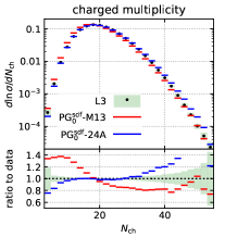
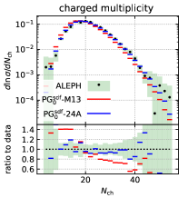
Figure 5: Results from the PG${}^{\text{sdf}}_{\beta_{\text{{ps}}}=0}$ NNLL parton shower, supplemented with Pythia 8.311 hadronisation, compared to a range of data, using both the PG${}_{0}^{\text{sdf}}$-24A and the PG${}_{0}^{\text{sdf}}$-M13 tunes from Table 2. The two tunes have identical perturbative parameters, but different non-perturbative parameters and the plots illustrate that predictions for infrared safe observables (top three rows) are largely unaffected by the change in non-perturbative parameters, except at the edge of the perturbative region.

Table 2 shows the non-perturbative parameters of Pythia 8.311 that have been tuned relative to the default Monash 2013 tune [84]. The tunes are based on ALEPH [82, 79] and L3 [83] data and have been produced with our own proof-of-concept tuning framework.

In addition to modifying non-perturbative parameters, we also take $\alpha_{s}(M_{Z})=0.1180$ with a 3-loop running coupling. In contrast, the Monash 2013 tune uses $\alpha_{s}(M_{Z})=0.1365$ with a 1-loop running coupling. Note that the latter does not include a $K_{1}$ contribution. If one interprets $\alpha_{s}(M_{Z})=0.1365$ as a CMW-scheme coupling, the corresponding $\overline{\textsc{ms}}$ value would be $\alpha_{s}^{\overline{\textsc{ms}}}(M_{Z})=0.1276$.

To appreciate the impact of the non-perturbative parameter choices, Fig. 5 shows results with the PG${}^{\text{sdf}}_{\beta_{\text{{ps}}}=0}$ shower and two tunes from Table 2: the Monash13 tune (PG${}_{0}^{\text{sdf}}$-M13, with $\alpha_{s}(M_{Z})=0.1180$) and the dedicated tune presented here (PG${}_{0}^{\text{sdf}}$-24A). (results for the other showers are broadly similar). For infrared safe observables (top three rows) the impact of the change in parameters is negligible except (a) where experimental uncertainties grow large and (b) deep in the 2-jet region where the Sudakov suppression involves non-perturbative physics. This gives confidence that the broad agreement that we see for these observables has not simply been artificially engineered by the tuning of the non-perturbative parameters. For all observables in the top two rows and the Thrust Major on the third row, our showers bring NNLL accuracy. The remaining observables on the third row, i.e. the Thrust minor, $y_{34}$ and $y_{45}$ have the property that they are non-zero starting only from four or more particles and for these we do not claim NNLL accuracy. Agreement remains generally good, though notably in the $4$ and $5$-jet regions this is at least in part accidental, given the lack of corresponding fixed-order matrix elements in the shower. For infrared unsafe observables (bottom row), such as the distribution of the number of charged tracks ($N_{\text{ch}}$), the particle momentum distribution ($\xi_{p}=-\ln(2|\vec{p}|/Q)$) or the rapidity of particles with respect to the Thrust axis ($y_{T}$), the tunes have a significant impact.

We stress that this tuning exercise should be considered as exploratory. For example, we have not made any effort to address the question of theory uncertainties. From a perturbative viewpoint, we do not include any heavy-quark effects (all quarks, including charm and bottom, are treated as massless). Also, we have made no efforts to tune the non-perturbative parameters affecting the rates of various identified particles ($\pi^{0}$, $\pi^{\pm}$, $K$, etc…). Nevertheless, this tuning exercise does show that the good agreement with infrared safe LEP $Z$-pole observables is not significantly affected by variations of the non-perturbative parameters and that distributions sensitive to non-perturbative physics improve after tuning.