Neural Representations of Dynamic Visual Stimuli

Jacob Yeung
Carnegie Mellon University
jjyeung@andrew.cmu.edu
Andrew F. Luo
Carnegie Mellon University
afluo@cmu.edu
Gabriel Sarch
Carnegie Mellon University
gsarch@andrew.cmu.edu
Margaret M. Henderson
Carnegie Mellon University
mmhender@cmu.edu
Deva Ramanan
Carnegie Mellon University
deva@andrew.cmu.edu
Michael J. Tarr
Carnegie Mellon University
michaeltarr@cmu.edu

Abstract

Humans experience the world through constantly changing visual stimuli, where scenes can shift and move, change in appearance, and vary in distance. The dynamic nature of visual perception is a fundamental aspect of our daily lives, yet the large majority of research on object and scene processing, particularly using fMRI, has focused on static stimuli. While studies of static image perception are attractive due to their computational simplicity, they impose a strong non-naturalistic constraint on our investigation of human vision. In contrast, dynamic visual stimuli offer a more ecologically-valid approach but present new challenges due to the interplay between spatial and temporal information, making it difficult to disentangle the representations of stable image features and motion. To overcome this limitation – given dynamic inputs, we explicitly decouple the modeling of static image representations and motion representations in the human brain. Three results demonstrate the feasibility of this approach. First, we show that visual motion information as optical flow can be predicted (or decoded) from brain activity as measured by fMRI. Second, we show that this predicted motion can be used to realistically animate static images using a motion-conditioned video diffusion model (where the motion is driven by fMRI brain activity). Third, we show prediction in the reverse direction: existing video encoders can be fine-tuned to predict fMRI brain activity from video imagery, and can do so more effectively than image encoders. This foundational work offers a novel, extensible framework for interpreting how the human brain processes dynamic visual information.

1 Introduction

From a car driving down the street to waves crashing against the shore, our daily lives are filled with visual stimuli that are constantly in motion. The dynamic and spatiotemporally rich nature of visual perception is a cornerstone of our daily experience, and the human visual system has evolved to extract meaningful patterns from the dynamics of the visual environment. Yet, dynamics have often been omitted in the study of the neural basis of high-level visual perception, with static images being the primary focus of many studies. Such inputs only capture a snapshot of the visual world, omitting the rich temporal information that is inherent in our everyday experiences. This omission is largely due to the relative computational simplicity of static images, which, while leading to significant advances in our understanding of the neural representations of visual features, has come at the cost of neglecting the dynamic aspects of visual perception. For example, a video of a person walking affords not only information about the visual features of the walker, but also about motion patterns, context, and relationships between the different elements in the scene (e.g., sudden increase in gait implies urgency). This interplay between spatial and temporal information may be impossible to capture from static images. Consequently, the neural responses evoked by dynamic visual stimuli are likely to differ from those evoked by static images, and understanding these differences is a significant challenge in developing a complete theory of visual perception.

In this paper, we propose a novel framework for analyzing dynamic visual stimuli, which explicitly decouples the modeling of static image representations and motion representations in the human brain. By doing so, we can provide a framework for studies that will enable a deeper understanding of how the brain processes dynamic visual stimuli. In particular, while some scene semantics are available from static images, dynamic visual perception is important to understanding ecologically critical domains such as social interaction and action representation. In the former domain, social roles are are often inferred through the relative physical motions of different actors [1] and in the latter domain, different actions often appear the same in static images, for example, opening versus closing a door, or standing up versus sitting down. For both, adding motion removes ambiguity.

Contributions. Our contributions are as follows. First, we demonstrate that visual motion information in the form of optical flow can be predicted (or decoded) from brain activity as measured by fMRI. Second, we show that this predicted motion can be used to realistically animate static images using a motion-conditioned video diffusion model (where the motion is driven by fMRI brain activity). We demonstrate that brain activity can produce more reliable animations than image-conditioned video diffusion models trained on massively-large datasets. Finally, we show prediction in the reverse direction: recent video encoders (such as VideoMAE and VC-1 [2, 3]) can more effectively predict fMRI brain activity from video imagery as compared to image encoders. Overall these results demonstrate the effectiveness of our approach as a novel, extensible framework for interpreting how the human brain processes dynamic visual information.

Refer to caption — Figure 1: Motion Prediction & Initial Frame Animation. We predict future optical flow fields using fMRI brain activity and the initial frame. We combine our predicted optical flow with a motion-conditioned video prior, DragNUWA, to animate the initial frame.

2 Related Work

Image decoding from fMRI

Reconstructing visual images from human brain activity, such as that measured by functional magnetic resonance imaging (fMRI), has significantly advanced through the use of deep learning models trained on extensive datasets of natural images [4, 5, 6, 7, 8, 9, 10, 11, 12, 13, 14, 15, 16]. Recently, the number of approaches that integrate various aspects of visual experiences to reconstruct visual perceptions has increased rapidly [17, 18, 19, 20, 21, 22, 23, 24, 25, 26, 27, 28]. This progress is largey due to the availability of large, publicly accessible fMRI datasets with well-annotated stimuli, such as BOLD5000 [29] and the Natural Scenes Dataset (NSD) [30], along with multimodal deep generative models that have been pre-trained on very large datasets, such as Stable Diffusion [31].

Video Decoding from fMRI

While there has been extensive decoding work on image reconstruction from fMRI, there has been much less work on video reconstruction. The most notable example of the latter is perhaps MindVideo [19], which performs pretraining to align temporal semantics from fMRI and simultaneously generate frames across time. Notably, our approach explicitly disentangles the representations of motion information (represented as optical flow) from static images in fMRI signals. This allows us to differentiate our present work from previous work by enabling interpretability. Specifically, we isolate and focus on decoding motion (as optical flow) from fMRI signals, as opposed to more difficult to interpret mixture of static image features and motion. This disentanglement allows us to learn an explicit representation of motion which can be directly compared to groundtruth and be more directly related to spatially localized neural mechanisms, as opposed to an entangled mixture of static image and dynamic features.

3 Methods

In order to understand how the brain processes dynamic visual stimuli, we focus on three directions. In the first, we examine the motion representation contained in the brain by decoding dense optical flow conditioned on the initial frame. In the second, we visualize the predicted motion by reconstructing the observed dynamic visual stimuli by leveraging a motion conditioned image diffusion model (DragNUWA). Finally, we examine which visual features, (static vs dynamic; semantic vs visual similarity) best explain brain activity on a voxel-wise level.

3.1 Motion Prediction

Our primary objective is to extract the information relevant to visual motion in order to predict the optical flow in videos observed by subjects. To enhance interpretability, we’ve architecturally separated static image features from dynamic features. By conditioning the model on the initial frame alongside neural data, we enable our model to focus on extracting dynamic visual information. This approach improves interpretability compared to models like MindVideo, which simultaneously predict both dynamic and static features. In contrast, our approach disentangles the specific contributions of dynamic components.

At a given fMRI scan at index $i$ we have fMRI voxels $B_{i}\in\mathbb{R}^{n}$ and corresponding video frames $\mathcal{I}_{i}\in\mathbb{R}^{T\times H\times W\times 3}$ . We obtain optical flow fields $O_{i}\in\mathbb{R}^{(T-1)\times H\times W\times 2}$ from RAFT [32], which consist of $(T-1)\times H\times W$ optical flow vectors in $\mathbb{R}^{2}$ . Prior work [33] has found that reformulating optical flow prediction as classification improves performance. We take a similar approach and quantize the optical flow vectors into a codebook of $k$ clusters using k-means. We obtain image features with pretrained vision model $G$ . More concretely, we learn a function $M_{\theta}$ that classifies the fMRI voxels $B_{i}$ and image features of the corresponding initial frame $G(\mathcal{I}_{i,1})$ to the quantized future predicted optical flows fields: $M_{\theta}([B_{i},\mathcal{I}_{i,1}])\rightarrow O_{i}$

In order to focus our evaluation on salient objects in a scene, we apply masking using FlowSAM [34] to track and identify salient objects. Consistent with claims in their paper, we found this method was effective in identifying salient objects.

Visualizing the Predicted Motion. We can visualize the predicted motion by passing in the predicted optical flow field and the initial frame to a pretrained motion-conditioned video diffusion model, DragNUWA [35]. This allows us to generate the dynamic vision stimuli (observed by the subject) or (driving the neural response).

3.2 Visual Stimuli-To-Brain Encoding.

Here we describe a complementary approach to understanding dynamic visual stimuli processing in the brain. We consider models trained on different tasks:

1.
Static Image: These models are trained on static visual stimuli without guidance from dynamics. The features extracted can identify brain voxels that are semantically and spatially tuned.
1. (a)
  
  Supervised: ResNet-50 is trained on ImageNet to categorize images into semantic classes [36].
2. (b)
  
  Self-supervised: DINOv1 and DINOv2 are vision transformer-based models trained to learn similar representations for visually similar patches of images without supervision on semantic similarity [37, 38].
3. (c)
  
  Semantically-supervised: CLIP (ViT-B-32) and CLIP ConvNeXt are trained to learn align semantics and images. CLIP uses a visual transformer architecture and CLIP ConvNeXt uses a convolutional backbone, sharing inductive biases with ResNet-50 but trained with a different objective. CLIP AF and CLIP ConvNeXt AF consist of CLIP and CLIP ConvNeXt features averaged over frames spanning the video [39, 40].
2.
Video: These models are trained on dynamic visual stimuli. The features extracted can identify brain voxels that are spatially and dynamically tuned.
1. (a)
  
  Self-supervised: VideoMAE, VideoMAE Large, Hiera Base Plus, and Hiera Huge are vision transformer-based architectures trained on Kinetics 400 with a masked autoencoder loss. The encoder learns embeddings used for downstream video tasks like action recognition [2, 41].
2. (b)
  
  Semantically-supervised: X-CLIP is a CLIP model fine-tuned with cross-frame attention to learn temporal relations [42].
3.
Embodied AI: These models are trained to align representations of single frames across time for embodied AI visuomotor manipulation. The features extracted can identify brain voxels tuned to action representation.
1. (a)
  
  Self-supervised: VIP is a ResNet-50 based architecture trained on the large-scale human egocentric video dataset Ego4D. VC-1 is a vision transformer-based architecture trained on seven human egocentric video datasets, including Ego4D. For both models, we also test an encoder trained on features averaged over frames spanning the video (VIP AF and VC-1 AF [43, 3]).
2. (b)
  
  Semantically-supervised: R3M is a ResNet-50 based architecture trained on Ego4D to align frames that are close in time and semantically similar [44].

We train ridge regression models on visual stimuli features from different vision encoding models to predict fMRI voxel-wise responses.

4 Experiments

In this section, we describe the specific experiments we use to explore dynamic visual representations in the human brain. In 4.1, we describe the dataset and preprocessing used. In 4.2 we explore motion decoding (reconstruction) conditioned on initial image and brain information, and augment quantitative analysis with visualizations derived from a motion-conditioned diffusion model. Finally in 4.3 , we explore the performance of different visual backbones in predicting brain activations.

4.1 Dataset

We utilize the Dynamic Natural Vision dataset [45], a public fMRI dataset composed of brain responses from 3 participants viewing diverse naturalistic video clips. The dataset contains 11.5 hours of fMRI data, with the 3 subjects viewing the same videos. The fMRI data was recorded using a 3T MRI system with a 2 second TR and the videos were presented at 30 FPS. 18 8-minute videos were seen twice and 5 8-minute videos were seen 10 times, including the train and test sets which have no overlapping videos. We use the same train/test split described in [45]. The fMRI data is preprocessed and aligned with presented stimuli using the pipeline from the Human Connectome Project. We further normalized the fMRI activations so that each voxel’s response was zero-mean and unit variance on a session basis. Then we average the response across repeated viewings of the same visual stimuli.

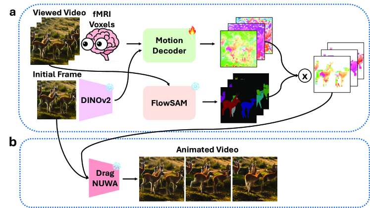
In practice, we temporally downsample the flows to $c=3$ frames, selected in equal intervals over the corresponding 2 second fMRI brain scan, and aim to predict the $c$ quantized consecutive optical flow fields. We also spatially downsample the flow to a resolution of $32\times 32$ and quantize the flows into 40 clusters. We extract image features from the first frame using DINOv2. During test time, we take a weighted-sum over all the classes per pixel, following [33]. We train the model using cross entropy loss. We train all models on a single Nvidia Titan RTX with 24GB GPU RAM and 48GB CPU RAM for up to 12 hours. We illustrate our model’s pipeline in Figure 2.

fMRI captures the blood oxygen level dependent (BOLD) signal, which peaks approximately 4 seconds after stimulus presentation and slowly decays after, due to nature of the hemodynamic response. During preprocessing, the fMRI data is shfited to temporally align the peak of the response to the onset of its corresponding visual stimuli presentation. However, due to the long time scale of the fMRI response, fMRI scans 4 seconds or 2 TRs prior and after the current TR may have information shared with the current TR. In order to leverage all relevant neural responses, when predicting the motion in the video presented at TR= $i$ , we concatenate fMRI data from TRs $[i-2,i-1,i,i+1,i+2]$ . We generate the video frames conditioned on the predicted motion using DragNUWA [35].

4.2 Motion Decoding

Quantitative Flow Evaluation.

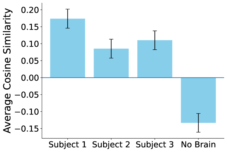
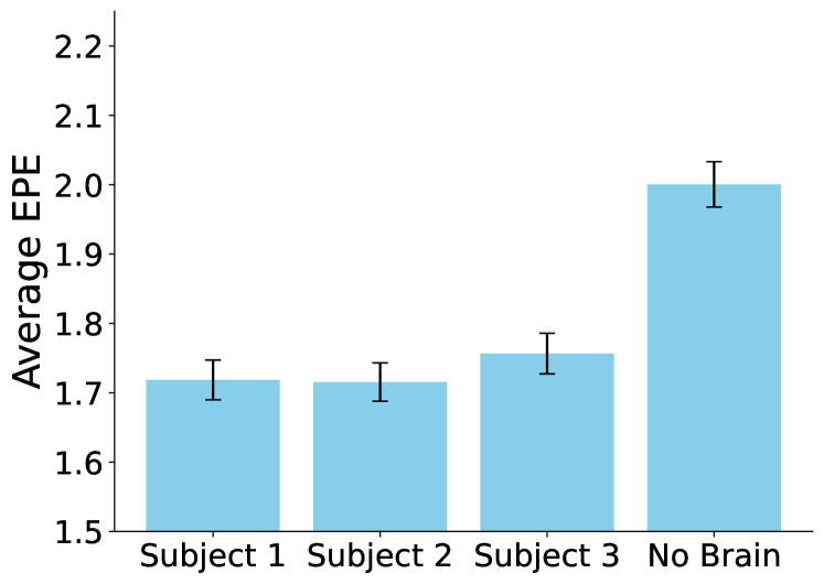
First we report evaluations of the decoded optical flow vectors on both direction and end point error on the test set. We quantitatively compare the models trained on the 3 subjects against a baseline of the motion decoder that does not use neural data and only image features from DINOv2 in Figure 3. Since this baseline model is not conditioned on neural data, the model learns to regress plausible flows which do not necessarily align with the true flow. Indeed, we observe that the models trained on neural data perform significantly better on both end point error ([ $1.72,1.72,1.76$ ] vs $2.00$ , $p\ll 0.001$ for the three models trained on neural data) and cosine similarity ([ $0.174,0.0854,0.1103$ ] vs $-0.133$ , $p\ll 0.001)$ . In addition, across the testing dataset, we find that models trained on neural data predict directions that are positively aligned with the true flow directions. In contrast, the model trained without neural data predicts flow directions that are actually anti-aligned with the true flow directions.

Reasoning With and Without fMRI.

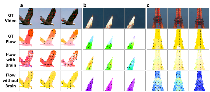
Here we present examples and explain why the models trained on neural data outperform the model trained without neural data (Figure 4).

First, there exists ambiguity of action given static images - a frame may contain multiple possible actions. For instance, in Figure 4a we show an eagle flying. Given the first frame, the eagle could be plausibly either flapping its wings or gliding. The model trained on neural data is able to identify that the eagle is gliding. However, the model trained without neural data incorrectly predicts that the eagle is flapping its wings. Second, even if the action is not ambiguous, there exists camera motion in the videos which can change the direction of the flow fields. For example, in Figure 4b we show a space shuttle flying into the sky. In this case, with no camera motion the direction of motion is clearly upwards and to the right, which the model trained without neural data correctly predicts. However, because the video is centered on the space shuttle with camera motion, the exhaust from the space shuttle appears to be going downwards and to the left. This causes the optical flow vectors to point downwards and to the left. Again, the model trained with neural data is able to correctly predict the motion of the object. Third, there exists ambiguity of direction of motion in static images of stationary objects. For instance, if the first frame contains just a stationary portion of the Eiffel Tower, what movement should be predicted? One could choose to predict no motion, or arbitrarily predict a direction of camera motion. Indeed, we see in Figure 4c that the trained model without neural data chooses an arbitrary camera motion pointing leftwards. However, the model trained with neural data correctly predicts the true direction which is camera panning downwards.

The results derived from these scenarios indicate that the neural data contains information about the correct movement which cannot be derived from just image features.

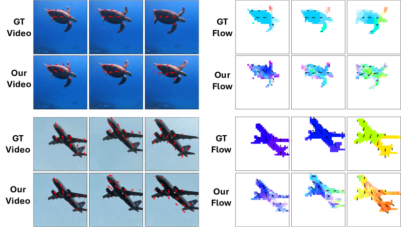
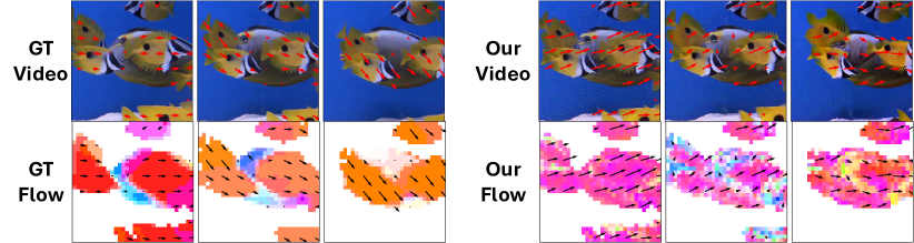
We show additional motion decoding results along with the video reconstruction from DragNUWA (Figure 5). We find that the motion we predict from the fMRI brain activity is not only aligned with the ground truth motion, but also generates realistic videos. We further demonstrate that we are able to decode motion that is consistent and that suddenly changes direction, i.e. the airplane example in Figure 5.

4.3 Identifying Brain Regions Tuned to Dynamic Features

Having demonstrated the ability to predict motion from fMRI brain activity, we now aim to identify brain regions selective for dynamic visual features. To do so, we test various vision encoding models to determine which best predict the fMRI brain activity of subjects watching dynamic visual stimuli. Specifically, we extract visual features using these models and construct voxel-wise encoding models using ridge regression [46, 47, 48, 49]. These voxel-wise encoding models predict the fMRI brain activity of subjects watching dynamic visual stimuli based on the extracted features.

Importantly, we test models spanning multiple visual properties, such as image versus video and semantic versus visual similarity, to help identify the brain’s functional properties. By analyzing the differences in encoding capabilities, we can identify brain regions more selective to dynamic visual features.

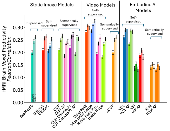
We find that the best performing video encoding model, VideoMAE Large, outperforms the best static image encoding models at predicting fMRI brain activity (Subject 1: $0.285$ , Subject 2: $0.314$ , Subject 3: $0.324$ , $p\ll 0.001$ ). This suggests that fMRI data during video viewing contain dynamic information which is not captured in features from static images.

Within the image encoding models, we find that CLIP ConvNeXt predicts fMRI brain activity best across all three subjects (Subject 1: $0.219$ , Subject 2: $0.263$ , Subject 3: $0.272$ , $p\ll 0.001$ ), corroborating prior results [50] that guidance from semantics is useful for predicting brain responses to visual stimuli. We also find that incorporating temporal information by averaging embeddings over multiple frames from encoding models that are not trained to be aligned over time does not improve performance.

We also find that the best performing embodied AI vision encoding models, VC-1, outperforms the best static image encoding models at predicts fMRI brain activity (Subject 1: $0.260$ , Subject 2: $0.290$ , Subject 3: $0.294$ , $p\ll 0.001$ ). Interestingly, VC-1 has been found to be better performing than the other embodied AI vision encoding models on average across a series of tasks [3]. This suggests a possible avenue of ranking embodied AI vision encoding models on predicting fMRI brain activity.

These results suggest that models which explicitly model temporal relationships are better at capturing neural responses to dynamic visual stimuli.

Interpreting Feature Performance.

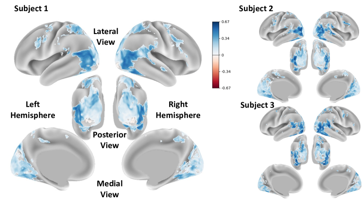
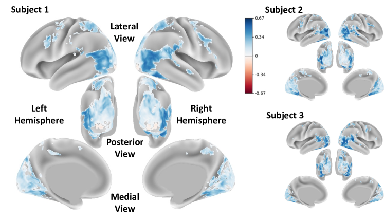
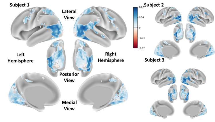
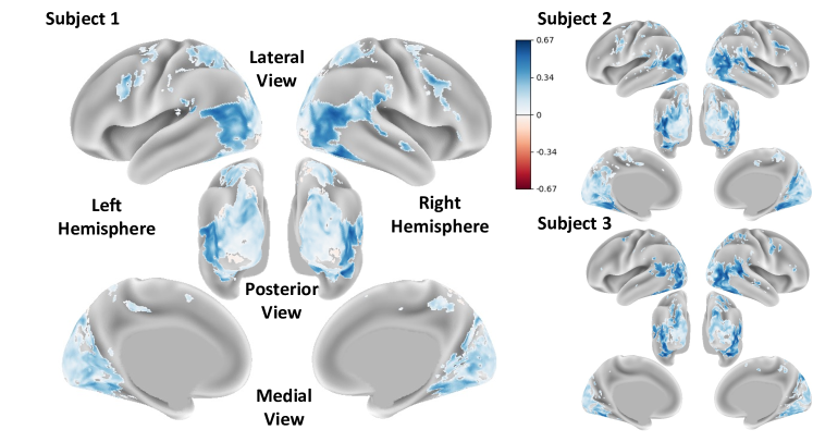
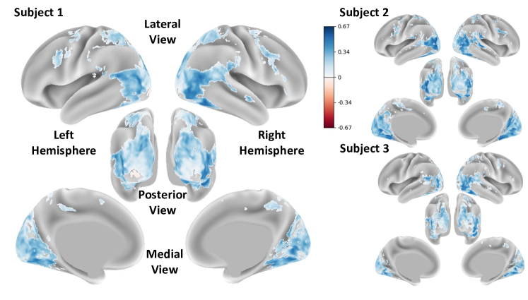
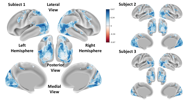
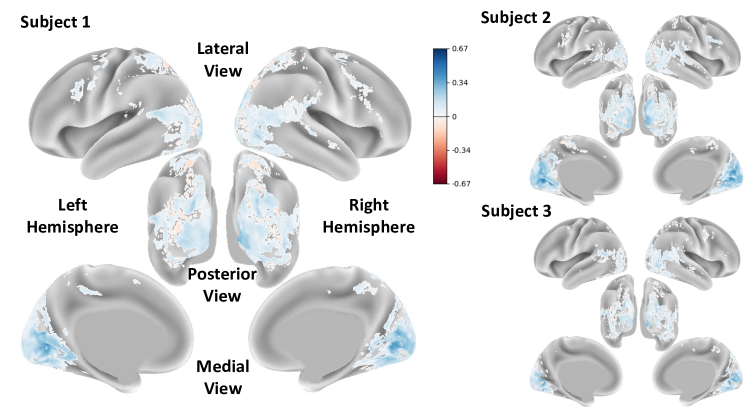
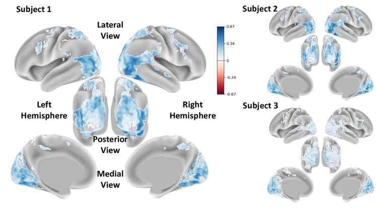
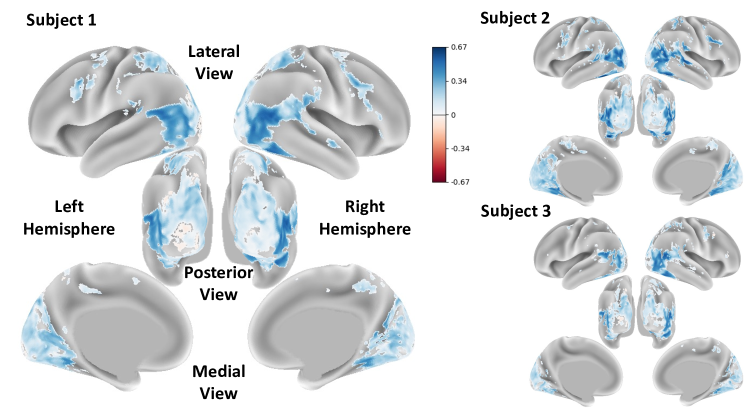
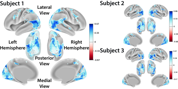
We plot voxel-wise encoding performance of the best performing model, VideoMAE, on an inflated cortical map to interpret the voxel-wise selectivity for dynamic visual stimuli features in Figure 7. Please refer to the caption for more detailed analysis. We identify fMRI brain voxels that are motion selective by taking the voxel-wise encoding performance difference between the best encoding video model, VideoMAE Large, and the best encoding static image model, CLIP ConvNeXt, illustrated in Figure 8. We find results that suggest encoding visual stimuli with VideoMAE better predicts fMRI brain activity across visual cortex and in somatosensory cortex. Additionally, we show the voxel-wise encoding performance of all models on inflated cortical maps in the supplementary information.

5 Conclusion

Limitations and Future Work.

Our methods successfully decode motion of salient objects from fMRI brain activity on the Dynamic Vision Dataset [45]. However, the generalizability of our conclusions to different dataset distributions remains unclear. Future datasets with fine-grained motion can help determine the limits of motion decodability from fMRI brain activity. Furthermore, our subject-specific training approach could be improved by exploring cross-subject alignment methods, as has been shown to improve decoding performance for static stimuli [54, 55].

Conclusion and Impact.

To summarize, in this paper we propose to study neural representations of motion by disentangling the modeling of static image features and motion. We show that brain activity can be used to predict visual motion, demonstrate that our predicted motion can animate static images to reconstruct the observed dynamic visual stimuli, and identify regions in the brain that are tuned for dynamic stimuli. Our results lay the groundwork for better understanding how the brain represents visual motion, and may help researchers construct better brain-machine interfaces.

References

Heider and Simmel [1944] F. Heider and M. Simmel. An experimental study of apparent behaviour. American Journal of Psychology, 13, 1944.
Tong et al. [2022] Zhan Tong, Yibing Song, Jue Wang, and Limin Wang. VideoMAE: Masked autoencoders are data-efficient learners for self-supervised video pre-training. In Advances in Neural Information Processing Systems, 2022.
Majumdar et al. [2023] Arjun Majumdar, Karmesh Yadav, Sergio Arnaud, Yecheng Jason Ma, Claire Chen, Sneha Silwal, Aryan Jain, Vincent-Pierre Berges, Pieter Abbeel, Jitendra Malik, Dhruv Batra, Yixin Lin, Oleksandr Maksymets, Aravind Rajeswaran, and Franziska Meier. Where are we in the search for an artificial visual cortex for embodied intelligence? 2023.
Yamins et al. [2014] Daniel LK Yamins, Ha Hong, Charles F Cadieu, Ethan A Solomon, Darren Seibert, and James J DiCarlo. Performance-optimized hierarchical models predict neural responses in higher visual cortex. Proceedings of the national academy of sciences, 111(23):8619–8624, 2014.
Horikawa and Kamitani [2017] Tomoyasu Horikawa and Yukiyasu Kamitani. Generic decoding of seen and imagined objects using hierarchical visual features. Nature communications, 8(1):15037, 2017.
Kietzmann et al. [2019] Tim C Kietzmann, Courtney J Spoerer, Lynn KA Sörensen, Radoslaw M Cichy, Olaf Hauk, and Nikolaus Kriegeskorte. Recurrence is required to capture the representational dynamics of the human visual system. Proceedings of the National Academy of Sciences, 116(43):21854–21863, 2019.
Güçlü and van Gerven [2015] Umut Güçlü and Marcel AJ van Gerven. Deep neural networks reveal a gradient in the complexity of neural representations across the ventral stream. Journal of Neuroscience, 35(27):10005–10014, 2015.
Groen et al. [2018] Iris IA Groen, Michelle R Greene, Christopher Baldassano, Li Fei-Fei, Diane M Beck, and Chris I Baker. Distinct contributions of functional and deep neural network features to representational similarity of scenes in human brain and behavior. Elife, 7, 2018.
Wen et al. [2018] Haiguang Wen, Junxing Shi, Yizhen Zhang, Kun-Han Lu, Jiayue Cao, and Zhongming Liu. Neural encoding and decoding with deep learning for dynamic natural vision. Cerebral cortex, 28(12):4136–4160, 2018.
Kell et al. [2018] Alexander JE Kell, Daniel LK Yamins, Erica N Shook, Sam V Norman-Haignere, and Josh H McDermott. A task-optimized neural network replicates human auditory behavior, predicts brain responses, and reveals a cortical processing hierarchy. Neuron, 98(3):630–644, 2018.
Koumura et al. [2019] Takuya Koumura, Hiroki Terashima, and Shigeto Furukawa. Cascaded tuning to amplitude modulation for natural sound recognition. Journal of Neuroscience, 39(28):5517–5533, 2019.
Schrimpf et al. [2021] Martin Schrimpf, Idan Asher Blank, Greta Tuckute, Carina Kauf, Eghbal A Hosseini, Nancy Kanwisher, Joshua B Tenenbaum, and Evelina Fedorenko. The neural architecture of language: Integrative modeling converges on predictive processing. Proceedings of the National Academy of Sciences, 118(45):e2105646118, 2021.
Goldstein et al. [2022] Ariel Goldstein, Zaid Zada, Eliav Buchnik, Mariano Schain, Amy Price, Bobbi Aubrey, Samuel A Nastase, Amir Feder, Dotan Emanuel, Alon Cohen, et al. Shared computational principles for language processing in humans and deep language models. Nature neuroscience, 25(3):369–380, 2022.
Caucheteux and King [2022] Charlotte Caucheteux and Jean-Rémi King. Brains and algorithms partially converge in natural language processing. Communications biology, 5(1):1–10, 2022.
Schmitt et al. [2021] Lea-Maria Schmitt, Julia Erb, Sarah Tune, Anna U Rysop, Gesa Hartwigsen, and Jonas Obleser. Predicting speech from a cortical hierarchy of event-based time scales. Science Advances, 7(49):eabi6070, 2021.
Sun et al. [2023] Jingyuan Sun, Mingxiao Li, Zijiao Chen, Yunhao Zhang, Shaonan Wang, and Marie-Francine Moens. Contrast, attend and diffuse to decode high-resolution images from brain activities. arXiv preprint arXiv:2305.17214, 2023.
Takagi and Nishimoto [2023] Yu Takagi and Shinji Nishimoto. High-resolution image reconstruction with latent diffusion models from human brain activity. In Proceedings of the IEEE/CVF Conference on Computer Vision and Pattern Recognition, pages 14453–14463, 2023.
Zeng et al. [2023] Bohan Zeng, Shanglin Li, Xuhui Liu, Sicheng Gao, Xiaolong Jiang, Xu Tang, Yao Hu, Jianzhuang Liu, and Baochang Zhang. Controllable mind visual diffusion model. arXiv preprint arXiv:2305.10135, 2023.
Chen et al. [2023a] Zijiao Chen, Jiaxin Qing, and Juan Helen Zhou. Cinematic mindscapes: High-quality video reconstruction from brain activity. arXiv preprint arXiv:2305.11675, 2023a.
Ozcelik and VanRullen [2023] Furkan Ozcelik and Rufin VanRullen. Brain-diffuser: Natural scene reconstruction from fmri signals using generative latent diffusion. arXiv preprint arXiv:2303.05334, 2023.
Lin et al. [2022] Sikun Lin, Thomas Sprague, and Ambuj K Singh. Mind reader: Reconstructing complex images from brain activities. arXiv preprint arXiv:2210.01769, 2022.
Lu et al. [2023] Yizhuo Lu, Changde Du, Dianpeng Wang, and Huiguang He. Minddiffuser: Controlled image reconstruction from human brain activity with semantic and structural diffusion. arXiv preprint arXiv:2303.14139, 2023.
Scotti et al. [2023] Paul S Scotti, Atmadeep Banerjee, Jimmie Goode, Stepan Shabalin, Alex Nguyen, Ethan Cohen, Aidan J Dempster, Nathalie Verlinde, Elad Yundler, David Weisberg, et al. Reconstructing the mind’s eye: fmri-to-image with contrastive learning and diffusion priors. arXiv preprint arXiv:2305.18274, 2023.
Koide-Majima et al. [2023] Naoko Koide-Majima, Shinji Nishimoto, and Kei Majima. Mental image reconstruction from human brain activity. bioRxiv, pages 2023–01, 2023.
Gu et al. [2022] Zijin Gu, Keith Jamison, Amy Kuceyeski, and Mert Sabuncu. Decoding natural image stimuli from fmri data with a surface-based convolutional network. arXiv preprint arXiv:2212.02409, 2022.
Chen et al. [2023b] Zijiao Chen, Jiaxin Qing, Tiange Xiang, Wan Lin Yue, and Juan Helen Zhou. Seeing beyond the brain: Conditional diffusion model with sparse masked modeling for vision decoding. In Proceedings of the IEEE/CVF Conference on Computer Vision and Pattern Recognition, pages 22710–22720, 2023b.
Ferrante et al. [2023] Matteo Ferrante, Furkan Ozcelik, Tommaso Boccato, Rufin VanRullen, and Nicola Toschi. Brain captioning: Decoding human brain activity into images and text. arXiv preprint arXiv:2305.11560, 2023.
Liu et al. [2023] Yulong Liu, Yongqiang Ma, Wei Zhou, Guibo Zhu, and Nanning Zheng. Brainclip: Bridging brain and visual-linguistic representation via clip for generic natural visual stimulus decoding from fmri. arXiv preprint arXiv:2302.12971, 2023.
Chang et al. [2019] Nadine Chang, John A Pyles, Austin Marcus, Abhinav Gupta, Michael J Tarr, and Elissa M Aminoff. Bold5000, a public fMRI dataset while viewing 5000 visual images. Scientific Data, 6(1):1–18, 2019.
Allen et al. [2022a] Emily J. Allen, Ghislain St-Yves, Yihan Wu, Jesse L. Breedlove, Jacob S. Prince, Logan T. Dowdle, Matthias Nau, Brad Caron, Franco Pestilli, Ian Charest, J. Benjamin Hutchinson, Thomas Naselaris, and Kendrick Kay. A massive 7t fmri dataset to bridge cognitive neuroscience and artificial intelligence. Nature Neuroscience, 25:116–126, 1 2022a. ISSN 15461726.
Rombach et al. [2022] Robin Rombach, Andreas Blattmann, Dominik Lorenz, Patrick Esser, and Björn Ommer. High-resolution image synthesis with latent diffusion models. In Proceedings of the IEEE/CVF Conference on Computer Vision and Pattern Recognition, pages 10684–10695, 2022.
Teed and Deng [2020] Zachary Teed and Jia Deng. Raft: Recurrent all-pairs field transforms for optical flow, 2020.
Walker et al. [2015] Jacob Walker, Abhinav Gupta, and Martial Hebert. Dense optical flow prediction from a static image, 2015.
Xie et al. [2024] Junyu Xie, Charig Yang, Weidi Xie, and Andrew Zisserman. Moving object segmentation: All you need is sam (and flow). arXiv preprint arXiv:2404.12389, 2024.
Yin et al. [2023] Shengming Yin, Chenfei Wu, Jian Liang, Jie Shi, Houqiang Li, Gong Ming, and Nan Duan. Dragnuwa: Fine-grained control in video generation by integrating text, image, and trajectory, 2023.
He et al. [2015] Kaiming He, Xiangyu Zhang, Shaoqing Ren, and Jian Sun. Deep residual learning for image recognition, 2015.
Caron et al. [2021] Mathilde Caron, Hugo Touvron, Ishan Misra, Hervé Jégou, Julien Mairal, Piotr Bojanowski, and Armand Joulin. Emerging properties in self-supervised vision transformers. In Proceedings of the International Conference on Computer Vision (ICCV), 2021.
Oquab et al. [2023] Maxime Oquab, Timothée Darcet, Theo Moutakanni, Huy V. Vo, Marc Szafraniec, Vasil Khalidov, Pierre Fernandez, Daniel Haziza, Francisco Massa, Alaaeldin El-Nouby, Russell Howes, Po-Yao Huang, Hu Xu, Vasu Sharma, Shang-Wen Li, Wojciech Galuba, Mike Rabbat, Mido Assran, Nicolas Ballas, Gabriel Synnaeve, Ishan Misra, Herve Jegou, Julien Mairal, Patrick Labatut, Armand Joulin, and Piotr Bojanowski. Dinov2: Learning robust visual features without supervision, 2023.
Radford et al. [2021] Alec Radford, Jong Wook Kim, Chris Hallacy, A. Ramesh, Gabriel Goh, Sandhini Agarwal, Girish Sastry, Amanda Askell, Pamela Mishkin, Jack Clark, Gretchen Krueger, and Ilya Sutskever. Learning transferable visual models from natural language supervision. In ICML, 2021.
Cherti et al. [2023] Mehdi Cherti, Romain Beaumont, Ross Wightman, Mitchell Wortsman, Gabriel Ilharco, Cade Gordon, Christoph Schuhmann, Ludwig Schmidt, and Jenia Jitsev. Reproducible scaling laws for contrastive language-image learning. In Proceedings of the IEEE/CVF Conference on Computer Vision and Pattern Recognition, pages 2818–2829, 2023.
Ryali et al. [2023] Chaitanya Ryali, Yuan-Ting Hu, Daniel Bolya, Chen Wei, Haoqi Fan, Po-Yao Huang, Vaibhav Aggarwal, Arkabandhu Chowdhury, Omid Poursaeed, Judy Hoffman, Jitendra Malik, Yanghao Li, and Christoph Feichtenhofer. Hiera: A hierarchical vision transformer without the bells-and-whistles. ICML, 2023.
Ma et al. [2022] Yiwei Ma, Guohai Xu, Xiaoshuai Sun, Ming Yan, Ji Zhang, and Rongrong Ji. X-CLIP:: End-to-end multi-grained contrastive learning for video-text retrieval. arXiv preprint arXiv:2207.07285, 2022.
Ma et al. [2023] Yecheng Jason Ma, Shagun Sodhani, Dinesh Jayaraman, Osbert Bastani, Vikash Kumar, and Amy Zhang. Vip: Towards universal visual reward and representation via value-implicit pre-training, 2023.
Nair et al. [2022] Suraj Nair, Aravind Rajeswaran, Vikash Kumar, Chelsea Finn, and Abhinav Gupta. R3m: A universal visual representation for robot manipulation, 2022.
Wen et al. [2017] Haiguang Wen, Junxing Shi, Yizhen Zhang, Kun-Han Lu, Jiayue Cao, and Zhongming Liu. Neural Encoding and Decoding with Deep Learning for Dynamic Natural Vision. Cerebral Cortex, 28(12):4136–4160, 10 2017. doi: 10.1093/cercor/bhx268. URL https://doi.org/10.1093/cercor/bhx268.
Kay et al. [2008] Kendrick N Kay, Thomas Naselaris, Ryan J Prenger, and Jack L Gallant. Identifying natural images from human brain activity. Nature, 452(7185):352–355, March 2008. ISSN 1476-4687, 0028-0836. doi: 10.1038/nature06713. Epub 2008 Mar 5.
Sarch et al. [2023] Gabriel H Sarch, Michael J Tarr, Katerina Fragkiadaki, and Leila Wehbe. Brain dissection: fmri-trained networks reveal spatial selectivity in the processing of natural images. bioRxiv, pages 2023–05, 2023.
Naselaris et al. [2011] Thomas Naselaris, Kendrick N Kay, Shinji Nishimoto, and Jack L Gallant. Encoding and decoding in fmri. Neuroimage, 56(2):400–410, 2011.
Allen et al. [2022b] Emily J Allen, Ghislain St-Yves, Yihan Wu, Jesse L Breedlove, Jacob S Prince, Logan T Dowdle, Matthias Nau, Brad Caron, Franco Pestilli, Ian Charest, et al. A massive 7t fmri dataset to bridge cognitive neuroscience and artificial intelligence. Nature neuroscience, 25(1):116–126, 2022b.
Wang et al. [2023] A. Y. Wang, K. Kay, T. Naselaris, M. J. Tarr, and L. Wehbe. Better models of human high-level visual cortex emerge from natural language supervision with a large and diverse dataset. Nature Machine Intelligence, 5(12):1415–1426, 2023. doi: 10.1038/s42256-023-00753-y.
Baker et al. [2018a] C. M. Baker, J. D. Burks, R. G. Briggs, A. K. Conner, C. A. Glenn, K. N. Taylor, G. Sali, T. M. McCoy, J. D. Battiste, D. L. O’Donoghue, and M. E. Sughrue. A connectomic atlas of the human cerebrum-chapter 7: The lateral parietal lobe. Operative Neurosurgery (Hagerstown), 15(suppl_1):S295–S349, December 2018a. doi: 10.1093/ons/opy261.
Baker et al. [2018b] C. M. Baker, J. D. Burks, R. G. Briggs, J. R. Sheets, A. K. Conner, C. A. Glenn, G. Sali, T. M. McCoy, J. D. Battiste, D. L. O’Donoghue, and M. E. Sughrue. A connectomic atlas of the human cerebrum-chapter 3: The motor, premotor, and sensory cortices. Operative Neurosurgery (Hagerstown), 15(suppl_1):S75–S121, December 2018b. doi: 10.1093/ons/opy256.
Baker et al. [2018c] C. M. Baker, J. D. Burks, R. G. Briggs, J. Stafford, A. K. Conner, C. A. Glenn, G. Sali, T. M. McCoy, J. D. Battiste, D. L. O’Donoghue, and M. E. Sughrue. A connectomic atlas of the human cerebrum-chapter 4: The medial frontal lobe, anterior cingulate gyrus, and orbitofrontal cortex. Operative Neurosurgery (Hagerstown), 15(suppl_1):S122–S174, December 2018c. doi: 10.1093/ons/opy257.
Huang et al. [2023] S. Huang, L. Sun, M. Yousefnezhad, M. Wang, and D. Zhang. Functional alignment-auxiliary generative adversarial network-based visual stimuli reconstruction via multi-subject fmri. IEEE Transactions on Neural Systems and Rehabilitation Engineering, 31:2715–2725, 2023. doi: 10.1109/TNSRE.2023.3283405. Epub 2023 Jun 20.
Andreella et al. [2023] Angela Andreella, Livio Finos, and Martin A Lindquist. Enhanced hyperalignment via spatial prior information. Human Brain Mapping, 44(4):1725–1740, 2023.
Rolls et al. [2022] Edmund T. Rolls, Gustavo Deco, Chu-Chung Huang, and Jianfeng Feng. The human language effective connectome. NeuroImage, 258:119352, 2022. ISSN 1053-8119. doi: https://doi.org/10.1016/j.neuroimage.2022.119352. URL https://www.sciencedirect.com/science/article/pii/S1053811922004712.

Supplementary Material:
Neural Representations of Dynamic Visual Stimuli

Appendix A HCP Parcellation Map

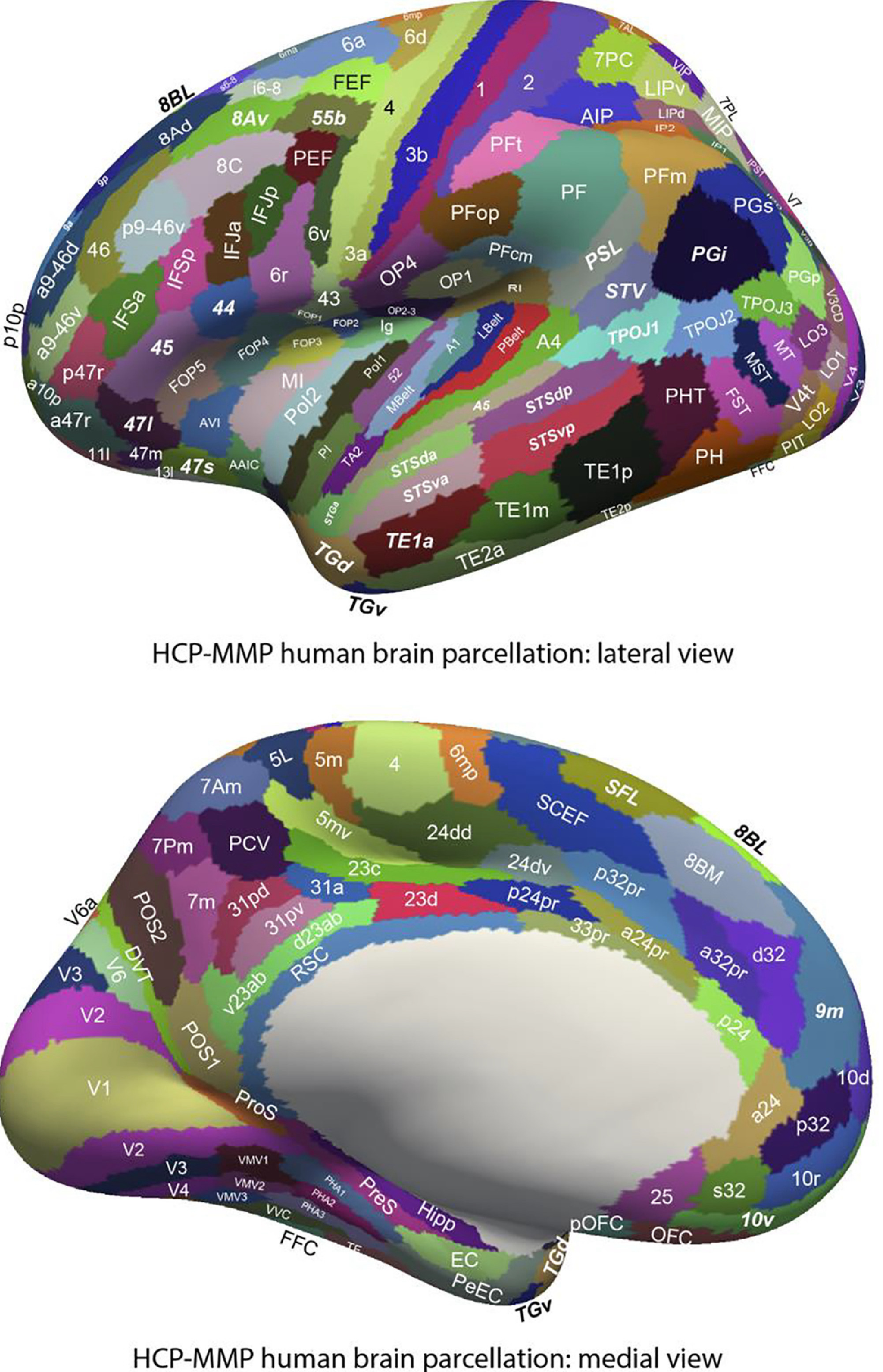
Here we show the parcellation (labeling) of the brain Figure 9.

Appendix B Additional Dataset Information

We use the Dynamic Vision Dataset collected by [45]. They release the dataset under a CC0 1.0 universal license. The url for the dataset can be found at https://purr.purdue.edu/publications/2805/1.

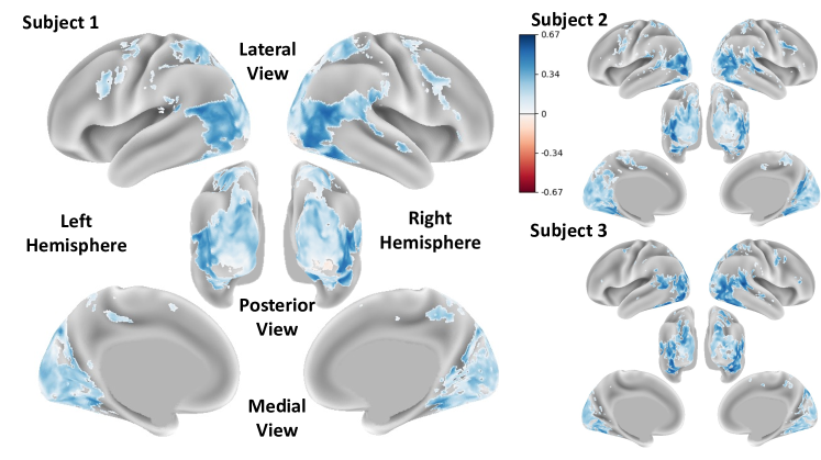
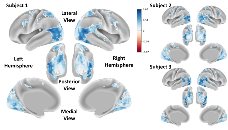
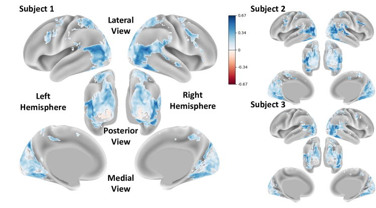
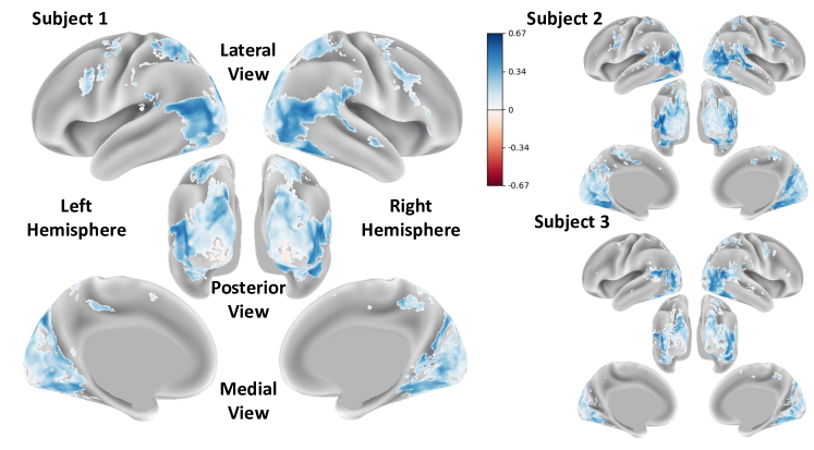
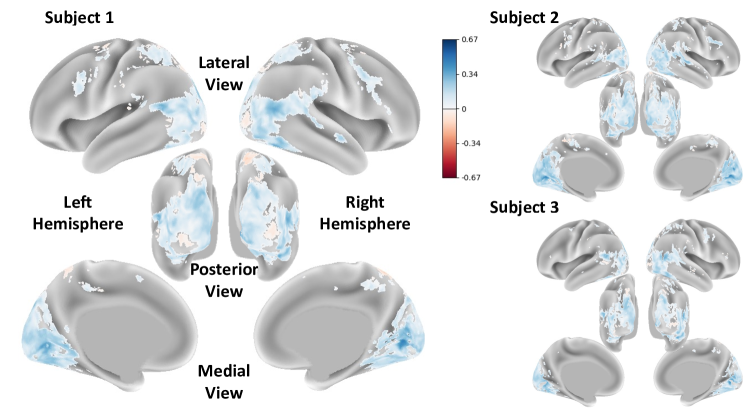
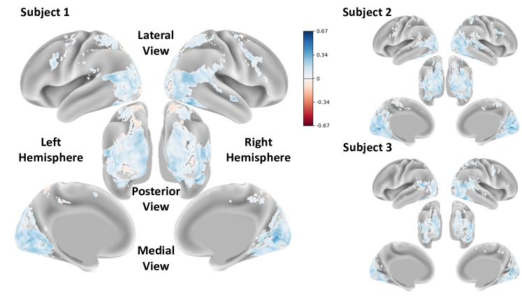
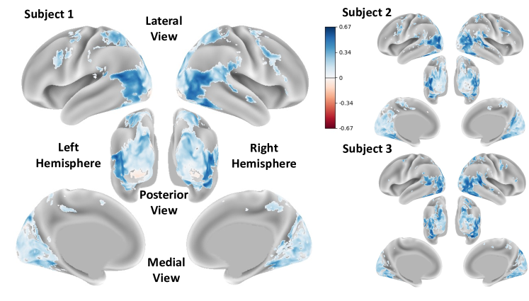
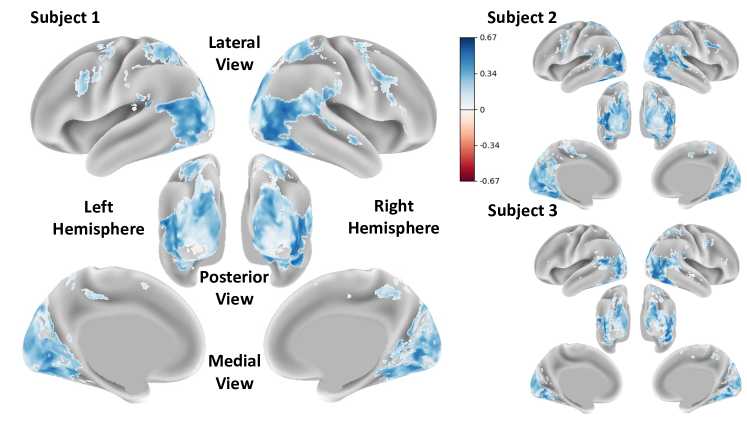
Appendix C Encoding Models Voxel-wise Prediction Performance on Inflated Cortex

Here we show the voxel-wise fMRI prediction performance, quantified as the Pearson correlation (r) between measured and predicted responses, for the remaining visual encoding models in alphabetical order.

Note that all following plots of encoding accuracy on inflated cortical maps are on the same scale for ease of comparison.