Exploring Effects of Hyperdimensional Vectors for Tsetlin Machines

Abstract

Tsetlin machines (TMs) have been successful in several application domains, operating with high efficiency on Boolean representations of the input data. However, Booleanizing complex data structures such as sequences, graphs, images, signal spectra, chemical compounds, and natural language is not trivial. In this paper, we propose a hypervector (HV) based method for expressing arbitrarily large sets of concepts associated with any input data. Using a hyperdimensional space to build vectors drastically expands the capacity and flexibility of the TM. We demonstrate how images, chemical compounds, and natural language text are encoded according to the proposed method, and how the resulting HV-powered TM can achieve significantly higher accuracy and faster learning on well-known benchmarks. Our results open up a new research direction for TMs, namely how to expand and exploit the benefits of operating in hyperspace, including new booleanization strategies, optimization of TM inference and learning, as well as new TM applications.

I Introduction

The success of an AI model depends on the internal representation of the data that the model considers. An appropriate representation allows the model to exploit the correct juxtaposition of the features available in the data to attain the best possible performance it is capable of. Moreover, in the case of interpretable AI models, this representation should also offer a one-to-one mapping between human-understandable features and features that are advantageous to the model. For Tsetlin machines, designing such feature spaces is referred to as data Boolanization, which is notoriously challenging for complex high-dimensional data, like sequences, graphs, images, signal spectra, and natural language. The reason is that the features must be natural building blocks for creating AND-rules that are both interpretable and accurate.

We here propose the hypervector Tsetlin machine (HVTM), which extends the capabilities of TMs by using hyperdimensional computing [1] with HV tokens. So-called binding operations combine tokens into more complex structures, while bundling operations assemble the resulting structures into a rich representation of the data. Accordingly, we preserve the uniqueness of the data while improving decision-making accuracy and efficiency.

The paper contributions can be summarized as follows:

• Our work introduces novel Booleanization strategies and hyperdimensional data analysis techniques based on the TM.

• We show how the TM can operate effectively in sparse hyperspaces, leveraging the capability of TMs to find non-linear patterns in high-dimensional spaces.

• We expose how a unique hyperparameter configuration where specificty $s$ is set to $1$, henceforth termed Reasoning by Elimination (RbE)  [2], is particularly suited for sparse hyperspaces.

• We further demonstrate the improvements achieved by the HVTM via experiments on multiple datasets in the domains of image processing, chemical structures identification and natural language processing (NLP).

• In each experiment, the HVTM is compared to the standard TM, to demonstrate their differences under the effect of various hyperparameter settings.

The paper is organized as follows. In Section II, we provide the details of HVTM, which we evaluate rigorously in Section III, contrasting it against the vanilla TM. Section IV concludes the paper by summarizing our findings and providing pointers to further work.

II Hypervector Tsetlin Machine

A HVTM extends the foundational principles of a standard TM into high-dimensional hyperspaces. Unlike traditional TMs that process Boolean inputs, a HVTM operates on Hyperboolean [3] inputs – complex constructs that emerge from operations within a hyperspace, effectively bypassing the limitations of a fixed-sized feature vector. The workflow of HVTM, as visualized in Figure 1, consists of the following steps, elaborated below.

Workflow of Hypervector Tsetlin Machine

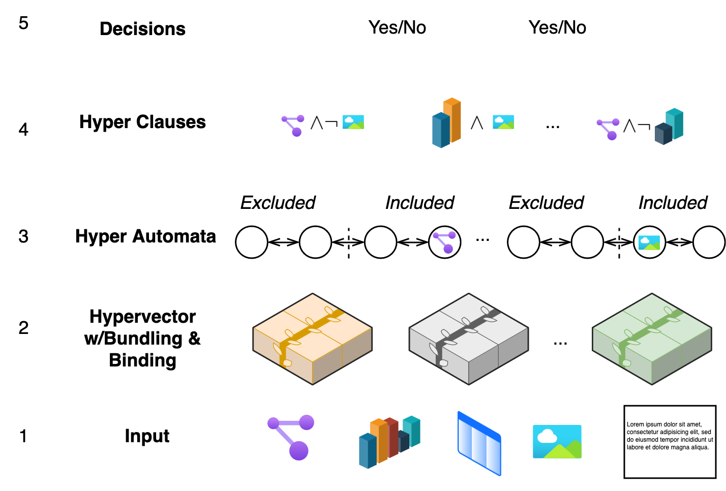
Figure 1: Tsetlin machine operating in hyperspace

1. Input Tokenization: Input data of various forms, such as text, images, or any complex data structure, is assigned a unique HV token, which is generated randomly.

2. Bundling and Binding Using bundling and binding techniques, we combine the tokens into high-dimensional vectors. HVs are thus made of hyper literals, each of which represents complex features of the input data.

3. Hyper Automata: Encoded HVs are then processed by a layer of hyper automata. Each hyper automaton functions identically to a Tsetlin automaton (TA), making decisions on whether to include or exclude a particular hyper literal.

4. Hyper Clauses: Hyper clauses are formed through the process of collective decision-making by the hyper automata. Each hyper clause represents a pattern or a rule that contributes to the decision-making process, and are the high-dimensional equivalent of conjunctive clauses in a standard TM.

5. Decisions: The hyper clauses finally vote for or against Yes/No output decisions according to how they match the input sample.

Following the above procedure, the HVTM is capable of handling high-dimensional data, making it applicable to a wider range of complex pattern recognition tasks, compared to the standard TM. The hyperspace operation allows for capturing intricate data relationships, potentially leading to more nuanced and sophisticated decision-making. How the HVTM processes HVs, in contrast to a regular TM operating on vectors, is explained in detail in the following section.

Hypervectors

A hyperspace gets arbitrarily high dimensionality by representing each dimension with a fixed-sized HV, typically of high dimensionality. Because of the fixed HV size, the hyperspace representation is lossy. However, increasing the HV size reduces the lossiness to any degree. Accordingly, HVs allows for a more complex and nuanced representation of data [4].

In our approach, we employ sparse HVs, which are binary/Boolean [1]. A sparse HV consists of a large fixed number of Booleans, e.g., $1024$, referred to as Hypervector size (HVSize) in the following. The HV gets a unique signature by setting a small number of the Booleans to True, randomly selected. These are referred to as the number of projection Booleans (NBits). We call the resulting HV as a token, representing a dimension in hyperspace. So, our first step is tokenization of the data, where each unique token forms a dimension. This process is pivotal in imparting complex meanings to the Booleans processed by the HVTM.

The synthesis of complex structures with sparse HVs is facilitated by operations known as Binding and Bundling. Binding involves a cyclic shift, effectively creating a new dimension in hyperspace, while Bundling is achieved through the logical OR operation, populating the hyperspace. This method of synthesis is crucial for creating new, unified hypervectors from existing ones [5].

Creation of a hypervector

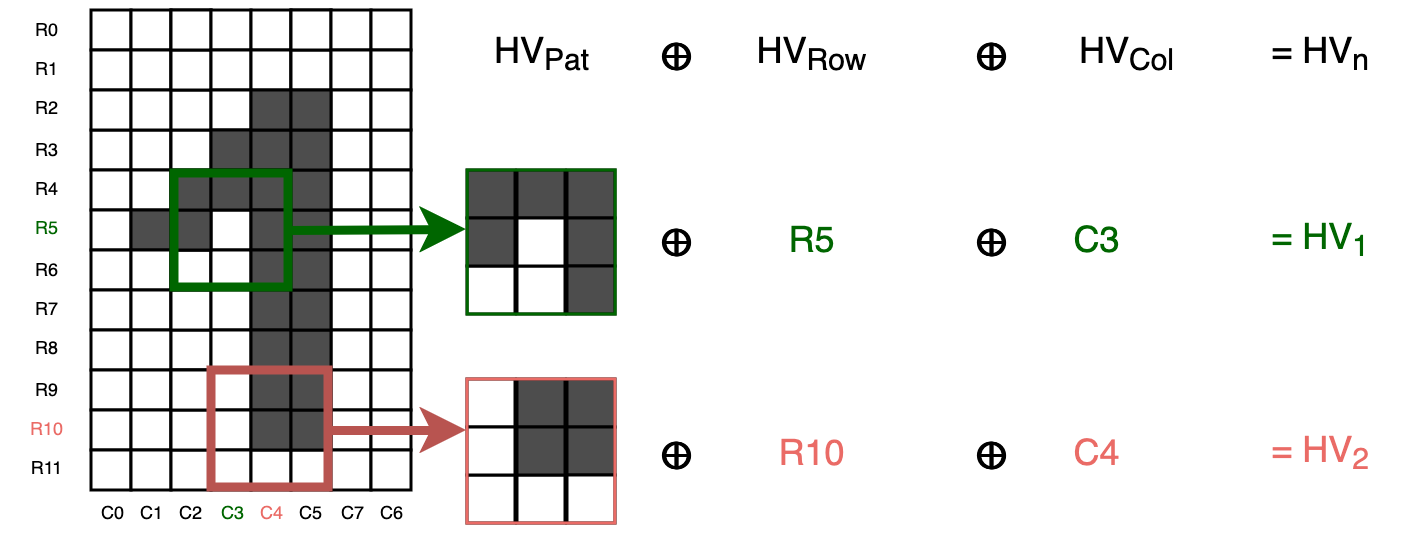
Figure 2: Creation of a Hypervector from 3 different hypervector tokens, bundling Patch with its respective Row and Column

Figure 2 illustrates the process of creating a HV within the HVTM framework, using an image example. The process begins by extracting a ‘Patch’ HV (HVPat) from the input image, which is represented as a grid of binary values, with black squares indicating a value of 1 and white squares a value of 0. This Patch is then bound with its corresponding ‘Row’ (HVRow) and ‘Column’ (HVCol) HVs, which are extracted based on the position of the Patch within the image (Row 5, Column 3 for HV1, and Row 10, Column 4 for HV2 in this example). The bundling operation involves a cyclic shift and logical OR, which combines these individual HVs to form a new, unified HV representing both the pattern and its position within the input space. For instance, HV1 is formed by bundling HVPat with R5 and C3, and similarly, HV2 with R10 and C4. This step-by-step combination of HVs is pivotal in encoding the spatial information of the Patch within the larger context of the image, thereby enhancing the data representation for subsequent processing by the HVTM.

Explainability

The HVTM, rooted in the principles of the TM, maintains its built-in capacity for understandable decision-making. Model’s reasoning can be decoded by breaking down hyperclauses, tracking individual hyperliterals carrying their specific meaning assigned during the encoding process. For example, in the Figure 3 we follow a clause extracted from the HVTM trained on the MNIST dataset. This clause contains both votes pro and against certain rows, columns and patches, which are the hyperfeatures that HVTM considers.

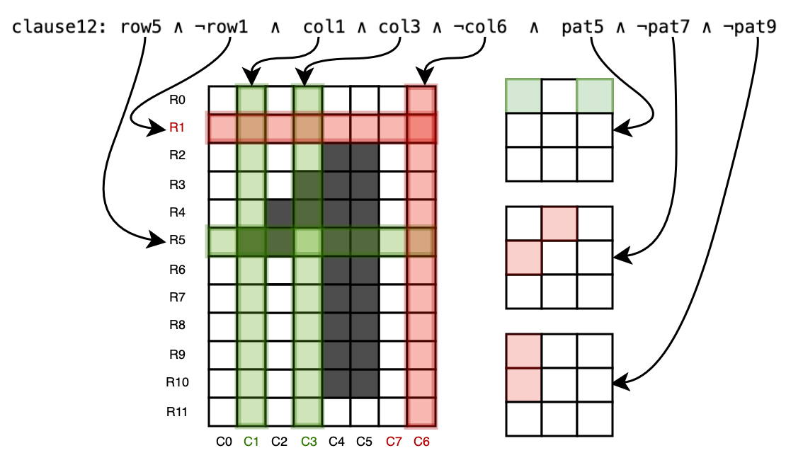
Figure 3: Interpretation of exported clauses after training, with hyperliterals representing rows, columns and different patches

In this context, the HVTM remains transparent and interpretable, allowing users to understand model decisions.

Dimensionality and Storage Limitations

Given the high-dimensional nature of HVs, the capacity of the HVTM to encode and differentiate between tokens is inherently linked to the hypervector size, denoted as $D$. This size restricts the maximum number of unique tokens that can be stored distinctly within the HVTM’s framework, where each token requires a certain quota of ’space’ or dimensions for its representation without ambiguity. The theoretical capacity $C$ of a HV to store unique tokens can be approximated, under ideal conditions, by the formula:

$$C\approx\frac{D!}{S!(D-S)!},$$

where $S$ represents the sparsity or the number of non-zero elements.

Projection Overlaps and Robustness

The token projection process aims to minimize overlaps. Nonetheless, when the diversity of input data or the token count surpasses the hypervector’s capacity, overlaps become inevitable. This reduces the HVTM’s robustness against overlaps, inversely proportional to the number of projection bits $P$. The likelihood $L$ of overlaps increases with the number of tokens $T$ relative to the hypervector size $D$, as shown by:

$$L=1-\left(1-\frac{1}{D^{P}}\right)^{T}.$$

Scalability and Computational Complexity

The scalability of HVTM is constrained by the dimensional size of hypervectors and the complexity of the Binding and Bundling operations. High-dimensional spaces necessitate more computational resources, potentially limiting the practical deployment of HVTM for large datasets or in resource-constrained environments.

To mitigate these limitations, further research is needed to optimize hypervector representations and develop more efficient algorithms for high-dimensional space management. This includes exploring adaptive or dynamic dimensionality adjustment mechanisms to balance storage capacity, token generation, and computational efficiency. Most promising research seems to be in Hardware Accelerators.

Understanding and addressing these limitations is crucial for advancing HVTM research towards more robust, scalable, and efficient models that leverage the benefits of high-dimensional computing while mitigating inherent challenges.

Internal mechanism of HVTM

A HVTM undertakes the task of binary classification for an input boolean HV $H=[h_{1},\ldots,h_{o}]$, where each $h_{i}$ represents a boolean hyperfeature. These hyperfeatures, along with their negated counterparts, form the hyperliterals pool, facilitating the HVTM’s processing.

For each target class, the HVTM constructs patterns using $n$ conjunctive hyperclauses, with $n$ being a predefined parameter by the user. Positive polarity is allocated to half of the clauses with an odd index, while negative polarity is assigned to the other half with an even index. The positive clauses carry information that supports the class, whereas the negative polarity clauses carry information that opposes the class. Each hyperclause, denoted as $C_{j}(H)$, is made up of a set of hyperliterals $L_{j}$ that are subsets of $L$, i.e. $L_{j}\subset L$. The clause $C_{j}(H)=h_{1}\land h_{2}=h_{1}h_{2}$, for example, comprises of the literals $L_{j}=\{h_{1},h_{2}\}$, $\bar{L_{j}}=\{\neg h_{1},\neg h_{2}\}$ and outputs $1$ if $h_{1}=h_{2}=1$.

The clause output is a measure of the certainty that a certain clause may contribute to the right classification decision. The unit step function is used to integrate the clause outputs into a classification decision through summation and thresholding using the unit step function $u(v)=1\leavevmode\nobreak\ \mathbf{if}\leavevmode\nobreak\ v\geq 0\leavevmode\nobreak\ \mathbf{else}\leavevmode\nobreak\ 0$:

$$\textstyle\hat{y}=u\left(\sum_{j=1}^{n/2}C_{j}^{+}(H)-\sum_{j=1}^{n/2}C_{j}^{-}(H)\right).$$ (1)

Namely, classification is done based on a majority vote, with the positive clauses voting for $y=1$ and the negative for $y=0$.

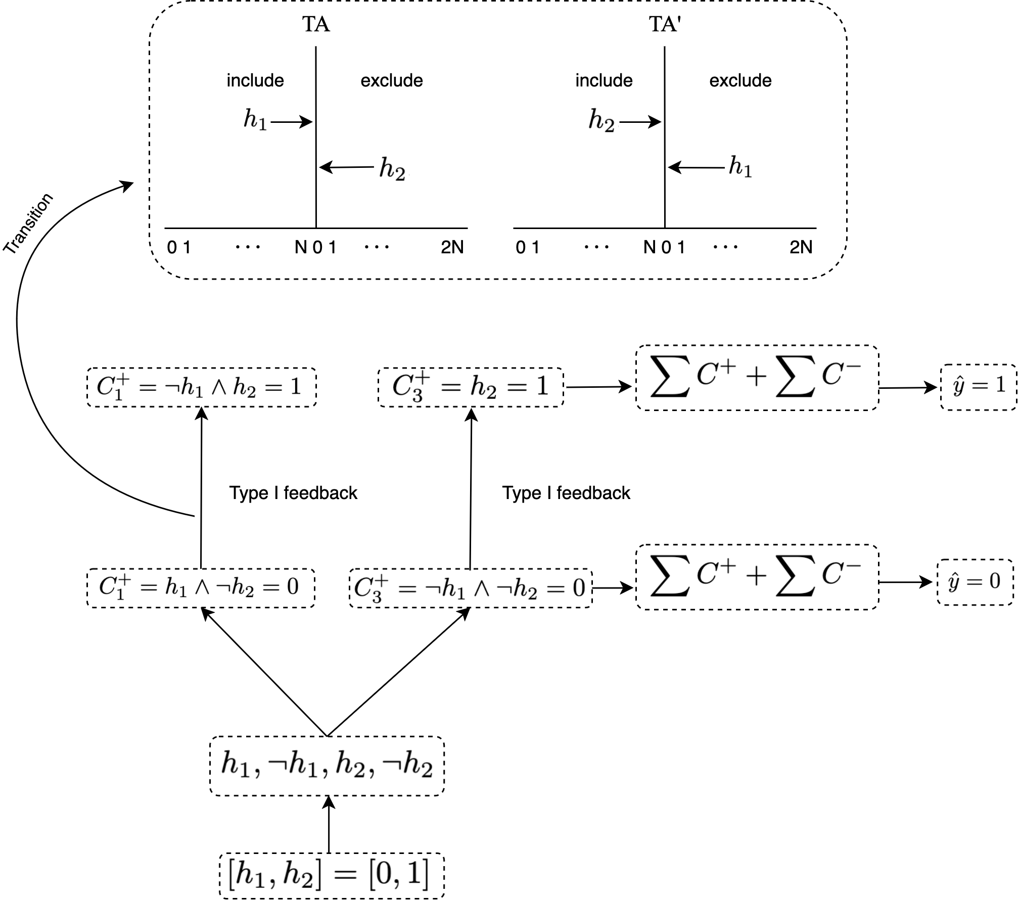
Figure 4: The learning of Tsetlin Machine for a sample of XOR gate.

A hyperclause $C_{j}(H)$ is created by a group of Hypervector Tsetlin Automatas [6], with each HVTA selecting whether to Include or Exclude a specific hyperliteral $l_{k}$ in the clause. The feedback TA receives in the form of Reward, Inaction, and Penalty is used to make decisions. TM provides two types of feedback: Type I Feedback and Type II Feedback, and their mechanism of application for the HVTM is the same as in a standard TM [7].

III Empirical Results

	Dataset Performance (%)
	TREC	HIV	IMDB	MNIST
HVTM	95.6	86.52	89.67	98.13
TM	91.6	85.57	86.61	97.2

TABLE I: Comparison of performance of HVTM vs TM, with identical parameters for both

Categorization of Natural Language Texts

In this section, we detail our experiments with Sparse HV to explore the HVTM in NLP in the context of the IMDB dataset [8] ($25000$ movie and series reviews), and the TREC dataset [9] ($5500$ question-answer pairs) fact-based question classification).

In IMDB, the highest accuracy rate achieved was 88.1% with HVSize of $8192$ and NBits as $4$ (Fig. 5). Fig. 6 shows that an optimal number of projection bits positively affects the accuracy, reaching a maximum of $88$% for $4$ bits with HVSize of $10000$. Using RbE further improves accuracy to $89.67$% (Fig. 7), while Fig. 8 shows that without RbE the maximum accuracy was 88.42%.

However, for TREC, highest accuracy of $96.8\%$ is achieved with a HVSize of $1024$ and NBits of $8$ given in Fig. 11, which presents heatmap of maximum accuracy for each NBits and HVSize. As NBits increases from $4$ (Fig. 9) to $16$ (Fig. 10), the HVTM exhibits increased stability though the accuracy remains similar.

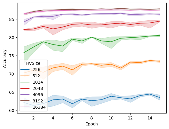
Figure 5: Sparse HV with varying HVSize for IMDB

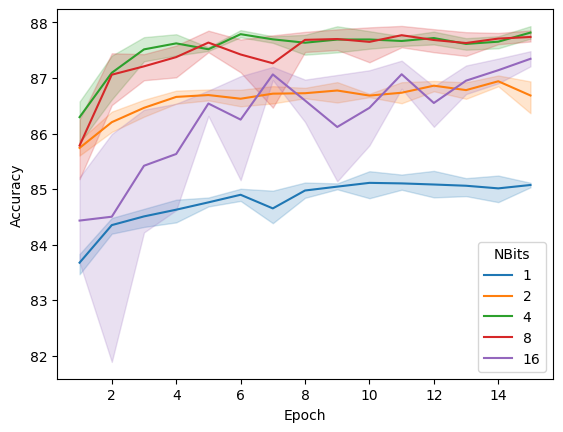
Figure 6: Sparse HV with varying NBits for IMDB

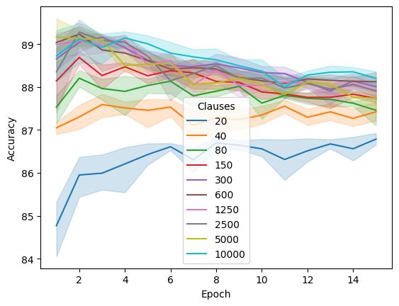
Figure 7: Sparse HV with RbE for IMDB

Figure 8: Sparse HV without RbE for IMDB

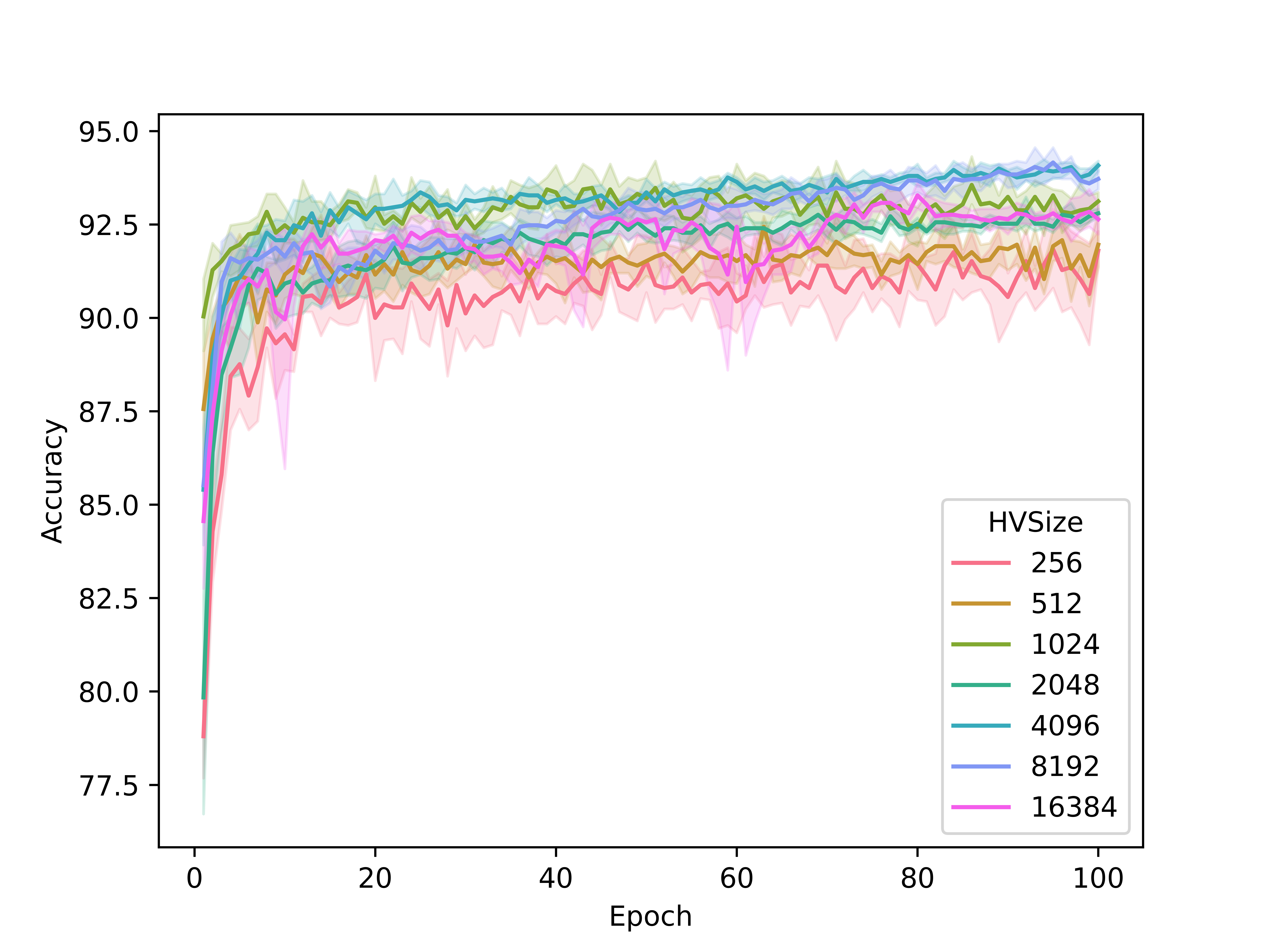
Figure 9: Accuracy versus training epochs of sparse HVTM for increasing HVSize on TREC dataset. NBits = 4.

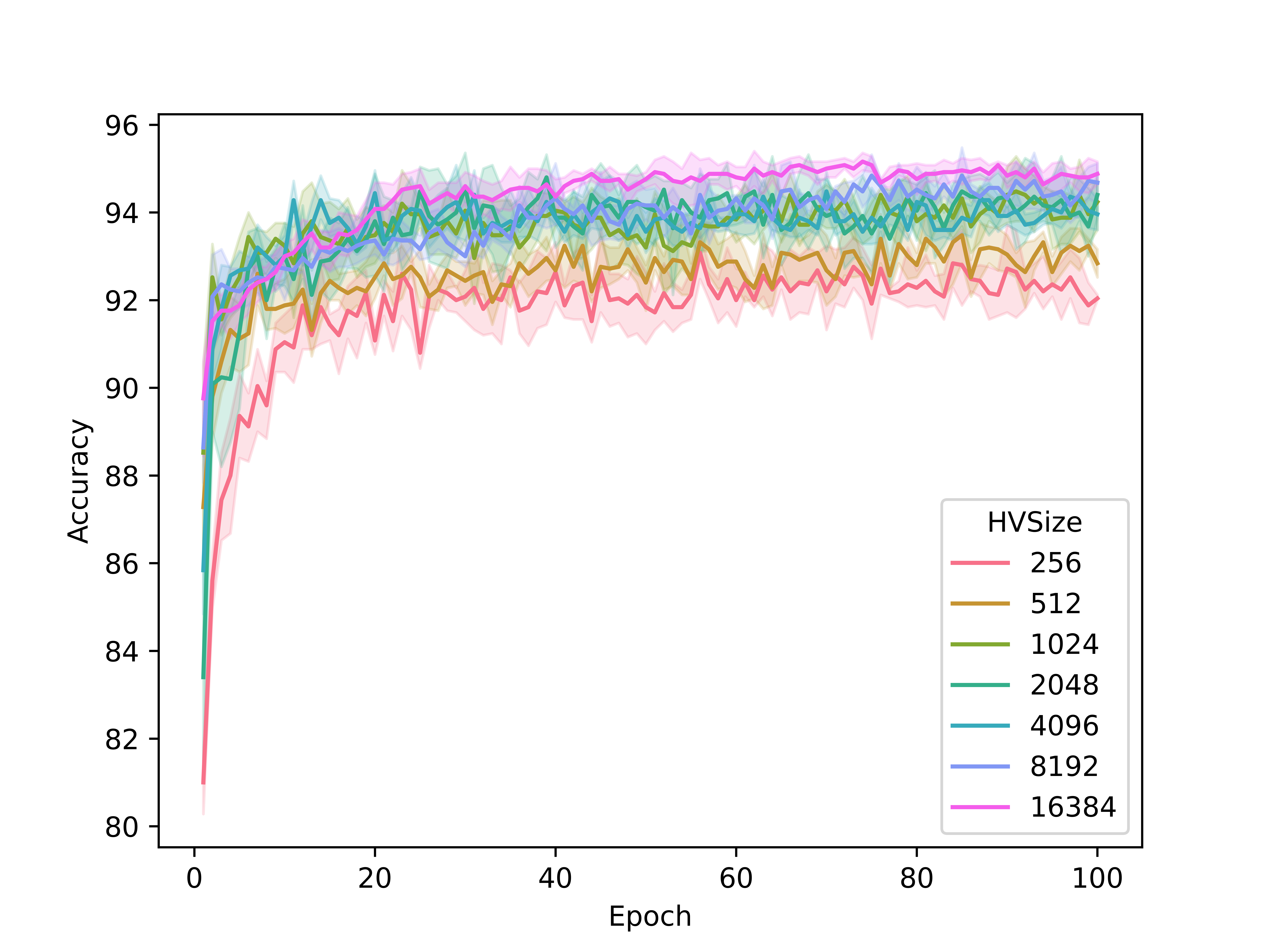
Figure 10: Accuracy versus training epochs of sparse HVTM for increasing HVSize on TREC dataset. NBits = 16

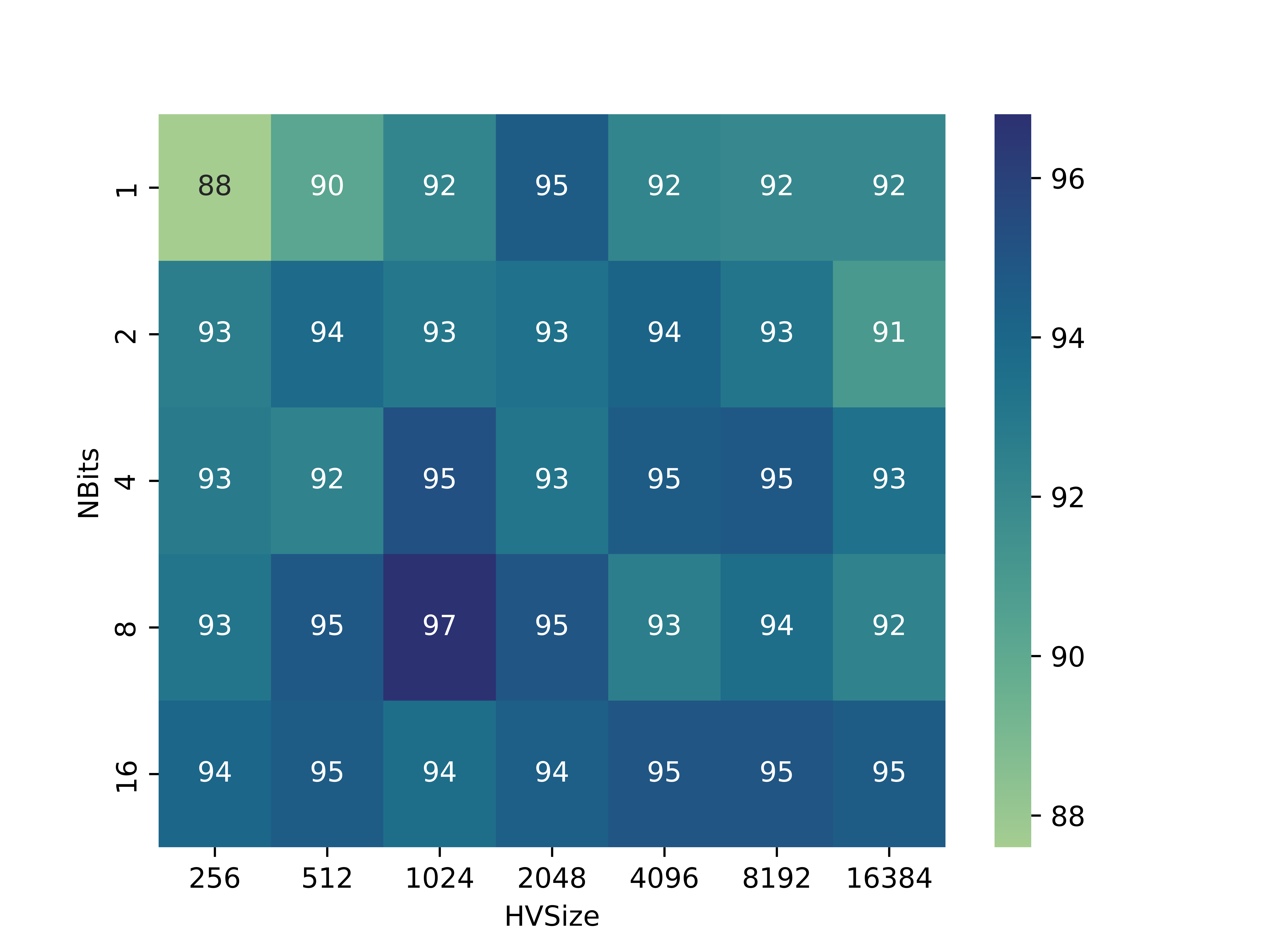
Figure 11: Heatmap of accuracy for sparse HVTM as a function of HV Size and the number of activated bits on TREC Dataset

Figure 12: Graceful degradation by decrease in number of clauses on TREC dataset

Classification of Compounds in Cheminformatics

The HIV dataset, introduced by the Drug Therapeutics Program (DTP) AIDS Antiviral Screen, tests the ability to inhibit HIV replication of $40000$ compounds [10]. Compounds are evaluated as: confirmed inactive (CI), confirmed active (CA) and confirmed moderately active (CM). For this work, we simplify the problem into a binary classification by merging the latter two labels, resulting in classes Inactive (CI) and Active (CA + CM). The HIV dataset is imbalanced with large numbers of inactive compounds ($39$, $684$) and few actives ($1$, $443$).

The presence and absence of 2D sub-structures for compounds of the HIV dataset are encoded using Extended Connectivity Fingerprints (ECFP) with a vector length of $4096$ and circular sub-structure graph radius of 3 bond-lengths (ECFP6) [11]. This initial feature set was used to build a conventional TM model to which the HVTM models are compared.

The ECFP6 sub-structure encodings were subsequently converted into HV representations of differing HVSizes and NBits. A given sub-structure bit position of the original ECFP6 features receives its own binary sparse HV, the description of a compound is then completed by a bit-wise disjunction operation across all present bit positions HVs. For each HVSize and NBits combination, a HVTM model was built and compared to each other via balanced accuracy (BalAccuracy) (Equation 2) [12]. This process was repeated 5 times with the mean values reported in Fig. 13.

$$BalancedAccuracy=\frac{\sum_{i}^{C}Recall_{i}}{N},$$ (2)

where $i$ is a given class, $C$ is the set of all classes and $N$ is the total number of classes.

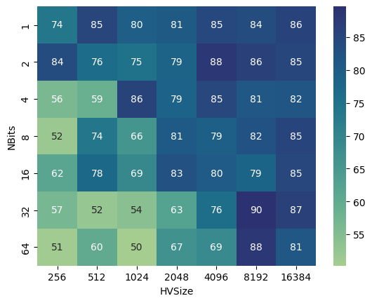
Figure 13: Heatmap of BalAccuracy for HVTM as a function of HVSizes and NBits on HIV Dataset

Fig. 13 shows that usually, the average balanced accuracy for classifying compounds as HIV active, across all NBits, increases with HVSize. Deviations from this trend can be seen, especially for the combinations: $1024$ HVSize with $4$ NBits, $8192$ HVSize and $32$ NBits. We hypothesize that bit collisions in the HV space allow the TM to create clauses which avail of sub-structure ”groups” encoded in a single HV Boolean position. These ideas are postulated by examining the balanced accuracy versus epoch curves (Fig. 14 and 15) of the NBits $4$ and $32$ respectively, and the corresponding cells in Fig. 13.

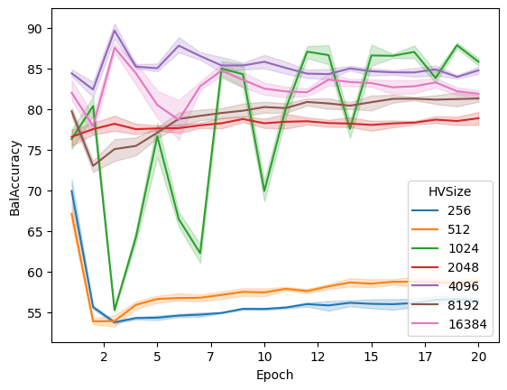
Figure 14: Balanced accuracy over training epochs of HVTM, for increasing HVSize, on chemical structures of HIV dataset. NBits=$4$.

Fig. 14 and Fig. 15 exhibit similar patterns, where low HVSizes prevent HVTMs from mining frequent patterns, until a certain HVSizes is reached and learning is volatile but ultimately accurate. At higher HVSizes, patterns in HV space were extracted quickly (after just 2 epochs) and with stable balanced accuracy ($86.52$%), more than that of $85.57$% achieved by the standard TM (Table I). In the case of NBits=$32$, it takes a much larger HVSizes ($\geq 8192$) to cross this threshold into stable learning for HVTMs compared to NBits=$4$ ($\geq 1024$). This is likely due to the greater number of bit collisions acting as noise when NBits is higher.

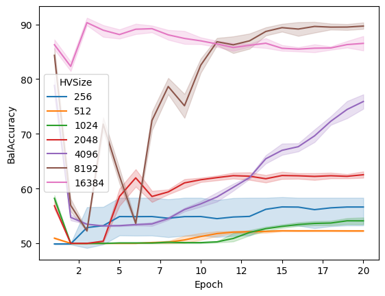
Figure 15: Balanced accuracy versus training epochs of HVTM, for increasing HVSizes, on HIV dataset. NBits=$32$

To reiterate, the high balanced accuracy achieved by the volatile HVTMs (NBits = $32$ and HVSize = $8192$, NBits = $4$ and HVSize = $1024$) after 20 epochs may be due to the grouping effect described earlier, where HVTMs use HV bit collisions of multiple sub-structure positions to effectively group and discriminate between compound sub-structures with their limited clause pool. This ”grouping” effect is just one of many potential hypotheses which will be examined in the future for chemical HVTM models.

Image Classification

We conduct a series of experiments on the MNIST dataset [13] to investigate the impacts of HVSize, NBits, and clause count on classification accuracy. To mitigate stochastic variations, each experimental condition was evaluated using five or more ensemble runs.

However, enforcing overlaps between HV tokens, for instance, aligning part of a token with specific columns or rows in the image (as in Figure 2), enhances overall accuracy despite the same HVSize (Fig. 16 shows the baseline results by Vanilla TM are surpassed).

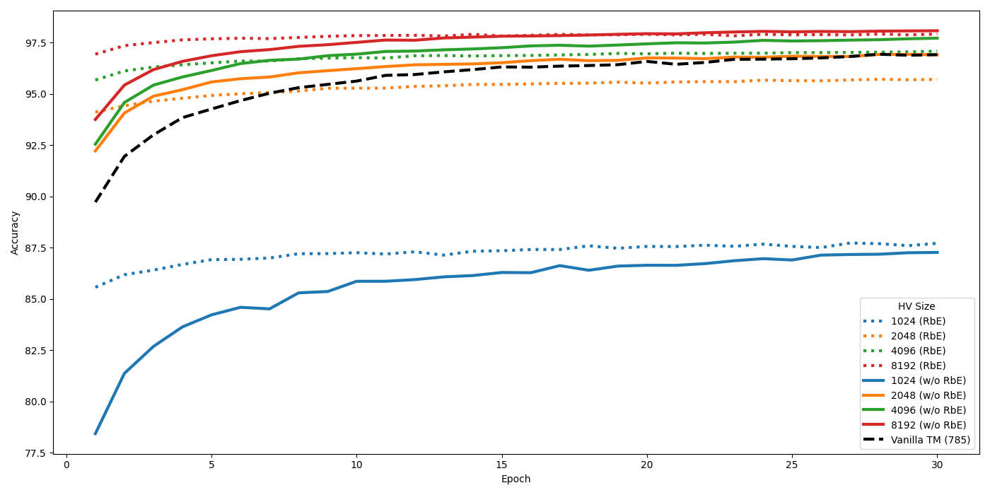
Figure 16: Comparing HVTM with RbE with varying HVSize and Vanilla TM

Fig. 16 also highlights the effect of HVSize. When the size is smaller than the amount of information we are trying to compress (note the 1024 bit HVSize in the figure), we get a lossy compression due to overlaps, resulting in a massive decrease in accuracy. Also observed in Figure 16 is the effect of using RbE. It seems to be faster in reaching higher accuracy in first few epochs, but eventually gets surpassed by the non-RbE setup.

Lastly, we examine the effect of reducing the number of clauses in a HVTM, which leads to graceful performance degradation (Fig. 17). Notably, even with a substantially more literals in the HVTM ($16384$ literals) versus in the traditional TM ($785$ literals), the HVTM achieves comparable performance with significantly fewer clauses. In the next Fig. 18, we see the detailed view of performance degradation due to reduced clause count in the HVTM on the MNIST dataset, employing RbE. What’s also interesting to note is the difference in variation among ensembles. The higher the number of clauses, the more stable is both the rise in performance and the performance itself.

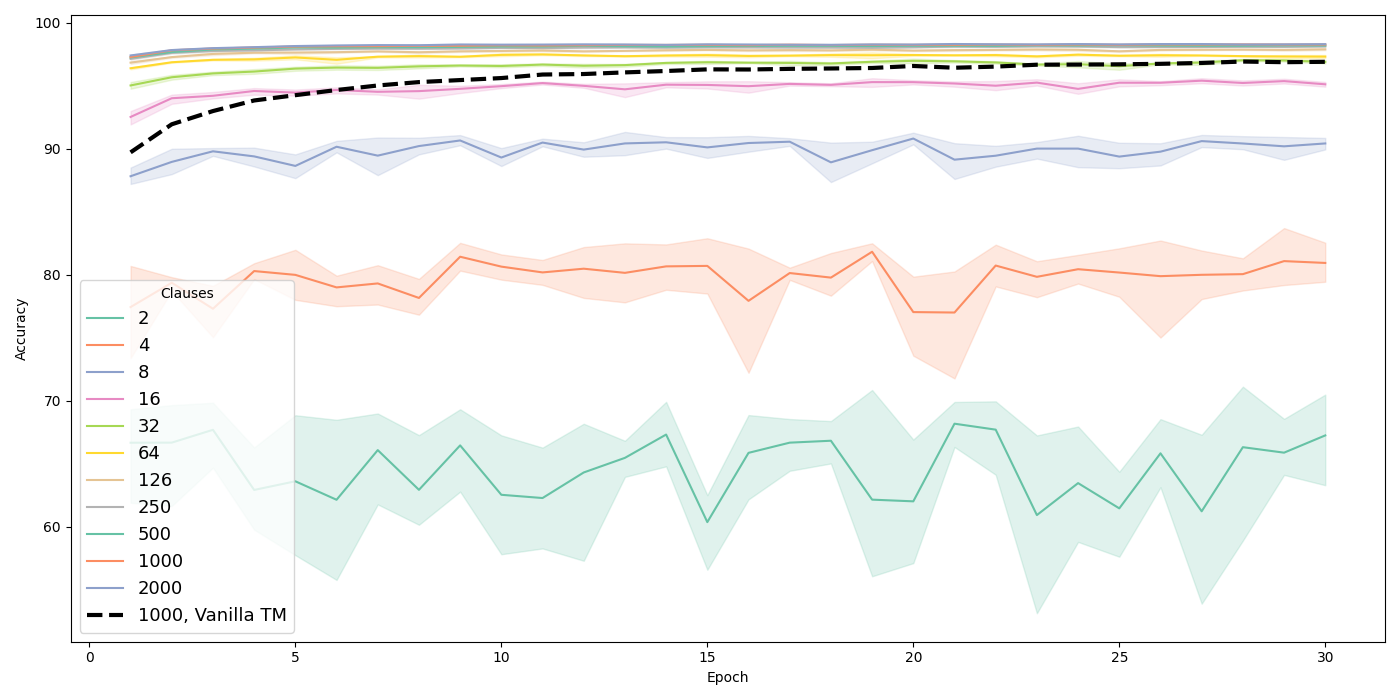
Figure 17: Performance degradation due to reduced clause count in the HVTM with RbE on the MNIST dataset

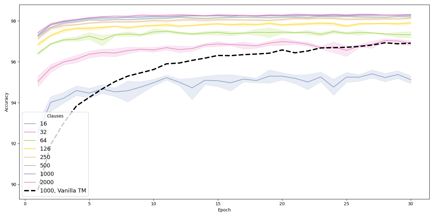
Figure 18: Detailed view of performance degradation due to reduced clause count in the HVTM on the MNIST dataset, using RbE.

IV Conclusion

In conclusion, this paper introduces the HVTM, a novel extension of the TM that leverages high-dimensional hypervectors to enhance Booleanization of complex data types and consequently the classification process. The HVTM demonstrates an improved capacity for both accuracy and learning speed, with reduced in clause numbers. This has been substantiated via experiments across the domains of text classification, image classification and cheminformatics.

HVTMs’ success in these domains underscores the potential of hyperdimensional computing, in conjunction with TM, to effectively manage and interpret complex data structures.

Future Work. This paper lays the foundation for further exploration in optimizing hyperspace utilization with Boolean Algebra. Key areas for future work include:

Refining the Binding and Bundling of HVs: These show great potential for encoding features into compact and easy to compute inputs. Not only do they expand the input space by extra dimensions while retaining feature information throughout the learning process, but also allow for constant transparency and interpretability. Leveraging HV overlaps can be explored via different combination and improvements on these techniques.

Expanding HV Applications in Cheminformatics: Currently, morgan fingerprint sub-graph bit positions have been simply converted into HV form. HV representations of compounds can be expanded upon in greater resolution by including bindings for each sub-substructure graph ECFP encoding and their number. This would allow variable length representations of compounds to be imprinted on fixed length HVs suitable for the HVTM. Similarly, 2D chemical graphs can be converted into HVs where each unique node (atom) and vertices (bond) is provided a sparse HV representation and bound together into sub-graph components. Through leveraging HVs, variable length graph-based TM models become feasible.

Exploring Reasoning by Elimination: In current experiments we observe that it creates clauses containing negative hyperliterals which point out what doesn’t belong to a certain class rather than focusing on specific hyperliterals which are true for such class. Further research is necessary to explore in detail how it affects the learning and subsequent interpretability across domains.

References

- [1] K. Schlegel, P. Neubert, and P. Protzel, “A comparison of vector symbolic architectures,” Artificial Intelligence Review, vol. 55, no. 6, pp. 4523–4555, 2022.
- [2] R. K. Yadav, J. Lei, O.-C. Granmo, and M. Goodwin, “Robust interpretable text classification against spurious correlations using and-rules with negation,” in International Joint Conferences on Artificial Intelligence. International Joint Conferences on Artificial Intelligence, 2022, pp. 4439–4446. [Online]. Available: https://hdl.handle.net/11250/3057374
- [3] V. Goranko and D. Vakarelov, “Hyperboolean algebras and hyperboolean modal logic,” Journal of Applied Non-Classical Logics, vol. 9, 01 1999.
- [4] S. Aygun, M. S. Moghadam, M. H. Najafi, and M. Imani, “Learning from hypervectors: A survey on hypervector encoding,” 2023.
- [5] T. Yu, Y. Zhang, Z. Zhang, and C. D. Sa, “Understanding hyperdimensional computing for parallel single-pass learning,” 2023.
- [6] M. L. Tsetlin, “On behaviour of finite automata in random medium,” Avtomat. i Telemekh, vol. 22, no. 10, pp. 1345–1354, 1961.
- [7] O.-C. Granmo, “The Tsetlin Machine - A Game Theoretic Bandit Driven Approach to Optimal Pattern Recognition with Propositional Logic,” arXiv preprint arXiv:1804.01508, 2018. [Online]. Available: https://arxiv.org/abs/1804.01508
- [8] D. Kaushik, E. H. Hovy, and Z. C. Lipton, “Learning the difference that makes a difference with counterfactually-augmented data,” CoRR, vol. abs/1909.12434, 2019. [Online]. Available: http://arxiv.org/abs/1909.12434
- [9] E. M. Voorhees and D. M. Tice, “Building a question answering test collection,” in Proceedings of the 23rd annual international ACM SIGIR conference on Research and development in information retrieval, 2000, pp. 200–207.
- [10] [Online]. Available: http://wiki.nci.nih.gov/display/NCIDTPdata/AIDS+Antiviral+Screen+Data
- [11] D. Rogers and M. Hahn, “Extended-connectivity fingerprints,” Journal of chemical information and modeling, vol. 50, no. 5, pp. 742–754, 2010.
- [12] K. H. Brodersen, C. S. Ong, K. E. Stephan, and J. M. Buhmann, “The balanced accuracy and its posterior distribution,” in 2010 20th International Conference on Pattern Recognition, 2010, pp. 3121–3124.
- [13] L. Deng, “The mnist database of handwritten digit images for machine learning research,” IEEE Signal Processing Magazine, vol. 29, no. 6, pp. 141–142, 2012.
- [14] G. T. Berge, O.-C. Granmo, T. O. Tveit, M. Goodwin, L. Jiao, and B. V. Matheussen, “Using the Tsetlin Machine to Learn Human-Interpretable Rules for High-Accuracy Text Categorization with Medical Applications,” IEEE Access, vol. 7, pp. 115 134–115 146, 2019.
- [15] K. D. Abeyrathna, O.-C. Granmo, X. Zhang, L. Jiao, and M. Goodwin, “The Regression Tsetlin Machine - A Novel Approach to Interpretable Non-Linear Regression,” Philosophical Transactions of the Royal Society A, vol. 378, 2020.
- [16] O.-C. Granmo, S. Glimsdal, L. Jiao, M. Goodwin, C. W. Omlin, and G. T. Berge, “The Convolutional Tsetlin Machine,” arXiv preprint arXiv:1905.09688, 2019. [Online]. Available: https://arxiv.org/abs/1905.09688
- [17] A. Wheeldon, R. Shafik, T. Rahman, J. Lei, A. Yakovlev, and O.-C. Granmo, “Learning Automata based Energy-efficient AI Hardware Design for IoT,” Philosophical Transactions of the Royal Society A, 2020.
- [18] A. Phoulady, O.-C. Granmo, S. R. Gorji, and H. A. Phoulady, “The Weighted Tsetlin Machine: Compressed Representations with Clause Weighting,” in Proceedings of the Ninth International Workshop on Statistical Relational AI (StarAI 2020), 2020.
- [19] S. Gorji, O. C. Granmo, S. Glimsdal, J. Edwards, and M. Goodwin, “Increasing the Inference and Learning Speed of Tsetlin Machines with Clause Indexing,” in International Conference on Industrial, Engineering and Other Applications of Applied Intelligent Systems. Springer, 2020.
- [20] S. R. Gorji, O.-C. Granmo, A. Phoulady, and M. Goodwin, “A Tsetlin Machine with Multigranular Clauses,” in Lecture Notes in Computer Science: Proceedings of the Thirty-ninth International Conference on Innovative Techniques and Applications of Artificial Intelligence (SGAI-2019), vol. 11927. Springer International Publishing, 2019.
- [21] K. D. Abeyrathna, O.-C. Granmo, and M. Goodwin, “Extending the Tsetlin Machine With Integer-Weighted Clauses for Increased Interpretability,” arXiv preprint arXiv:2005.05131, 2020. [Online]. Available: https://arxiv.org/abs/1905.09688
- [22] R. Shafik, A. Wheeldon, and A. Yakovlev, “Explainability and Dependability Analysis of Learning Automata based AI Hardware,” in IEEE 26th International Symposium on On-Line Testing and Robust System Design (IOLTS). IEEE, 2020.
- [23] C. D. Blakely and O.-C. Granmo, “Closed-Form Expressions for Global and Local Interpretation of Tsetlin Machines with Applications to Explaining High-Dimensional Data,” arXiv preprint arXiv:2007.13885, 2020. [Online]. Available: https://arxiv.org/abs/2007.13885
- [24] K. D. Abeyrathna, O.-C. Granmo, R. Shafik, A. Yakovlev, A. Wheeldon, J. Lei, and M. Goodwin, “A Novel Multi-Step Finite-State Automaton for Arbitrarily Deterministic Tsetlin Machine Learning,” in Lecture Notes in Computer Science: Proceedings of the 40th International Conference on Innovative Techniques and Applications of Artificial Intelligence (SGAI-2020). Springer International Publishing, 2020.
- [25] X. Zhang, L. Jiao, O.-C. Granmo, and M. Goodwin, “On the convergence of Tsetlin machines for the identity- and not operators,” arXiv preprint arXiv:2007.14268, 2020.
- [26] L. Jiao, X. Zhang, O.-C. Granmo, and K. D. Abeyrathna, “On the convergence of tsetlin machines for the xor operator,” arXiv preprint arXiv:2101.02547, 2021.
- [27] R. Yadav, L. Jiao, O.-C. Granmo, and M. Goodwin, “Human-level interpretable learning for aspect-based sentiment analysis,” AAAI, 2021.
- [28] X. Li and D. Roth, “Learning question classifiers,” in COLING 2002: The 19th International Conference on Computational Linguistics, 2002.
- [29] E. M. Voorhees, “Overview of the trec-9 question answering track,” in In Proceedings of the Ninth Text REtrieval Conference (TREC-9. Citeseer, 2001.
- [30] D. D. Lewis, “Reuters-21578 text categorization collection data set,” 1997.
- [31] R. Saha, O.-C. Granmo, and M. Goodwin, “Using tsetlin machine to discover interpretable rules in natural language processing applications,” Expert Systems, p. e12873, 2021.
- [32] D. Patterson, J. Gonzalez, U. Hölzle, Q. H. Le, C. Liang, L.-M. Munguia, D. Rothchild, D. So, M. Texier, and J. Dean, “The carbon footprint of machine learning training will plateau, then shrink,” 2022. [Online]. Available: https://doi.org/10.36227/techrxiv.19139645.v3
- [33] S. Glimsdal and O. Granmo, “Coalesced multi-output tsetlin machines with clause sharing,” CoRR, vol. abs/2108.07594, 2021. [Online]. Available: https://arxiv.org/abs/2108.07594
- [34] A. Radford, J. W. Kim, C. Hallacy, A. Ramesh, G. Goh, S. Agarwal, G. Sastry, A. Askell, P. Mishkin, J. Clark et al., “Learning transferable visual models from natural language supervision,” in International Conference on Machine Learning. PMLR, 2021, pp. 8748–8763.
- [35] T. Chen, S. Kornblith, M. Norouzi, and G. Hinton, “A simple framework for contrastive learning of visual representations,” in International conference on machine learning. PMLR, 2020, pp. 1597–1607.
- [36] Y. Kalantidis, M. B. Sariyildiz, N. Pion, P. Weinzaepfel, and D. Larlus, “Hard negative mixing for contrastive learning,” Advances in Neural Information Processing Systems, vol. 33, pp. 21 798–21 809, 2020.
- [37] A. Krizhevsky, G. Hinton et al., “Learning multiple layers of features from tiny images,” 2009.
- [38] C. Blake, “Uci repository of machine learning databases,” http://www. ics. uci. edu/~ mlearn/MLRepository. html, 1998.
- [39] P. Bachman, R. D. Hjelm, and W. Buchwalter, “Learning representations by maximizing mutual information across views,” Advances in neural information processing systems, vol. 32, 2019.
- [40] Z. Wu, Y. Xiong, S. X. Yu, and D. Lin, “Unsupervised feature learning via non-parametric instance discrimination,” in Proceedings of the IEEE conference on computer vision and pattern recognition, 2018, pp. 3733–3742.
- [41] F. Schroff, D. Kalenichenko, and J. Philbin, “Facenet: A unified embedding for face recognition and clustering,” in Proceedings of the IEEE conference on computer vision and pattern recognition, 2015, pp. 815–823.
- [42] J. D. Robinson, C.-Y. Chuang, S. Sra, and S. Jegelka, “Contrastive learning with hard negative samples,” in International Conference on Learning Representations, 2020.
- [43] K. D. Abeyrathna, B. Bhattarai, M. Goodwin, S. R. Gorji, O.-C. Granmo, L. Jiao, R. Saha, and R. K. Yadav, “Massively parallel and asynchronous tsetlin machine architecture supporting almost constant-time scaling,” in International Conference on Machine Learning. PMLR, 2021, pp. 10–20.
- [44] J. Sharma, R. Yadav, O.-C. Granmo, and L. Jiao, “Drop clause: Enhancing performance, interpretability and robustness of the tsetlin machine,” arXiv preprint arXiv:2105.14506, 2021.
- [45] C.-Y. Wu, R. Manmatha, A. J. Smola, and P. Krahenbuhl, “Sampling matters in deep embedding learning,” in Proceedings of the IEEE International Conference on Computer Vision, 2017, pp. 2840–2848.
- [46] B. Gunel, J. Du, A. Conneau, and V. Stoyanov, “Supervised contrastive learning for pre-trained language model fine-tuning,” arXiv preprint arXiv:2011.01403, 2020.
- [47] P. Khosla, P. Teterwak, C. Wang, A. Sarna, Y. Tian, P. Isola, A. Maschinot, C. Liu, and D. Krishnan, “Supervised contrastive learning,” Advances in Neural Information Processing Systems, vol. 33, pp. 18 661–18 673, 2020.
- [48] H. Steck, C. Ekanadham, and N. Kallus, “Is cosine-similarity of embeddings really about similarity?” arXiv preprint arXiv:2403.05440, 2024.
- [49] Images used for the figure: https://www.britannica.com/animal/beagle-dog, https://wp-rocket.me/blog/image-metadata-can-impact-web-performance-security/, https://learnopencv.com/histogram-of-oriented-gradients/.