Warm Inflation with Barrow Holographic Dark Energy
Abstract
In this work we study the warm inflation mechanism in the presence of the Barrow holographic dark energy model. Warm inflation differs from other forms of inflation primarily in that it makes the assumption that radiation and inflaton exist and interact throughout the inflationary process. After the warming process, energy moves from the inflaton to the radiation as a result of the interaction, keeping the cosmos warm. Here we have set up the warm inflationary mechanism using Barrow holographic dark energy as the driving agent. Warm inflation has been explored in a high dissipative regime and interesting results have been obtained. It is seen that the Barrow holographic dark energy can successfully drive a warm inflationary scenario in the early universe. Finally, the model has been compared with the observational data and compliance has been found.
1 Introduction
Big-bang model is the most successful model in modern cosmology. According to the standard Big Bang cosmological model [1, 2, 3], the universe is either radiation or matter-dominated, which should lead to a decelerated expansion of the universe. Despite its success, the Big Bang theory may be incomplete in its classic form because it is not sufficient to solve some cosmological problems such as the flatness problem, horizon problem, and also the magnetic monopole problem [4, 5, 6, 7, 8]. These cosmological issues can be explained by the concept of inflation which was first proposed by A. Guth in 1981 [5]. Following inflation, the universe will enter a reheating phase, in which the inflaton decays into light particles, thermalizing the universe. By considering the cosmic expansion history from the time when the observed CMB scales escape the Hubble boundaries during inflation to when they re-enter it at a later time, it is conceivable to establish a link between the parameters of inflation and reheating. A review of inflationary cosmology can be found in [9]. Other notable developments on cosmological inflation can be found in [10, 11, 12, 13, 14, 15].
The main idea of warm inflation [16] is that unlike cold inflation (the original inflation theory), there is an extra ”friction term” that acts as a regulator to fix the number density. In ordinary inflation, particle density exponentially reaches zero after inflation due to de-Sitter-type expansion. However, in warm inflation, we have specific characteristic temptation scales, such that the particle number does not go to zero due to coupling with another field. Warm inflation differs from other forms of inflation primarily in that it assumes that radiation and inflaton exist and interact throughout the inflationary process. After the warming process, energy moves from the inflaton to the radiation as a result of the interaction, keeping the cosmos warm. Consequently, warm inflation can lead to a very smooth phase of the universe, a radiation era, offering a novel solution to the graceful exit problem. Also, it should be noted that the cold inflation problem makes the flatness problem difficult to resolve. Warm inflation can naturally tackle the problem, hence offering much better reasoning for the flatness problem.
It should also be noted that just like cold inflation affects the curvature perturbation, which in turn reciprocates to the CMB anisotropy, for warm inflation, similar calculations have been performed in [17]. This shows that during the viscous warm inflation time scale (typically 16 to 60 e-fold timing), one can work with some models motivated by field theory and string theory, which can indeed give the bound on the viscosity parameter (in adiabatic approximations) [18]. A study of warm inflation in both weak and strong dissipative regimes have been performed by Moss and Berera [19, 20] and as a consequence, one can show how phenomenological quantities such as scalar power spectrum behaves as a function of the dissipative parameter [21].
To verify the warm inflation model with observation, there is a huge problem with the dissipation term, which maintains the equilibrium between the inflation field and the heat bath. The adiabatic approximation, which we use to maintain the equilibrium, would break down after the inflationary period (after 60 e-fold timing) as the characteristic mass of the radiation field is almost zero or negligible. So the scalar field perturbation would overshoot the approximation [22]. One way to circumvent this problem is to use the heavy super potential [23], which can be originated via brane-antibrane stacks in string theory [24] or extra-dimensional compactification like Kaluza-Klein theory [25]. This bound on the heavy potential and dissipation parameters has been given via analyzing WIMP data in [26]. Finally, we note that there is an alternative way to solve the radiation era problem by noting that we can consider the inflation field to be a pseudo-Nambu-Goldstone Boson field and during the radiation era the perturbation would not break down the approximation due to spontaneous symmetry breaking mechanism which is given in [27, 28]. For an overall review (with historical anecdotes) one can look into Berera’s article on warm inflation [29] and also Rangarajan’s article [30].
Holographic dark energy is an alternative theory of dark energy, where we attempt to apply the holographic principle to the dark energy problem. Gerard ’t Hoof proposed the holographic principle [31, 32] inspired by the investigation of black hole thermodynamics [33]. The relationship between a quantum field theory’s greatest length and its ultraviolet cutoff [34] can result in holographic vacuum energy, which forms dark energy on cosmological scales [35, 36]. The holographic principle states that all of the information contained in a volume of a space can be portrayed as a hologram, that corresponds to a theory lying on the boundary of that space. The concept of holographic principle has been widely used in various fields of physics such as in nuclear physics to study the problems of quark-gluon plasma [37], in the field of condensed matter to study the problems of quark-gluon plasma [38], in the field of theoretical physics that lead to the idea of holographic entanglement entropy[39], in the field of cosmology to discuss the nature of de-Sitter space and inflation [40]. The holographic principle states that the universe’s horizon entropy is proportional to its area, comparable to the Bekenstein-Hawking entropy of a black hole. This is a key step in applying it to cosmology. Applying the holographic principle to the dark energy framework, a new model of dark energy known as the Holographic dark energy model (HDE) is formed. Very recently inspired by the illustrations of the Covid-19 virus, Barrow [41] showed that quantum-gravitational effects introduce the fractal features on the black-hole structure that leads to finite volume with infinite area. The corresponding black-hole entropy can be expressed as
| (1.1) |
where is the standard horizon area , is the Planck area and is the deformation parameter. It should be noted that for , the Bekenstein–Hawking entropy is recovered while corresponds to the most intricate fractal structure. It is important to note that the aforementioned quantum-gravitationally corrected entropy differs from the standard ”quantum-corrected” entropy that uses logarithmic adjustments [42, 43], however, it resembles Tsallis nonextensive entropy [44, 45, 46], however, the underlying theories and physical concepts are entirely distinct. Lastly, take note that the aforementioned effective fractal behavior is based on broad, elementary physical principles rather than particular quantum gravity computations. This increases its believability and makes it a valid initial approach to the topic [41]. Saridakis in [47] used the extended Barrow relation for horizon entropy and constructed a holographic dark energy model known as the Barrow holographic dark energy (BHDE). Although BHDE possesses the usual holographic dark energy as a limit for , it is a novel scenario with a richer cosmological behavior and structure.
In [48] the author has studied a warm inflationary mechanism using the standard holographic dark energy and obtained very interesting results. Given the peculiar features of BHDE, we are motivated to explore a warm inflationary mechanism driven by the Barrow holographic dark energy. The fractal features inherent in BHDE are expected to produce very interesting results when incorporated in a warm inflationary mechanism. The work is organized as follows: In section 2 we discuss the warm inflationary mechanism. Section 3 is dedicated to the study of warm inflation with BHDE. Finally, the paper ends with some discussion and conclusion in section 4.
2 Warm Inflationary mechanism
We start with the two fundamental equations of cosmology i.e. the Friedmann equations,
| (2.1) |
| (2.2) |
where the subscripts ’r’ and ’in’ stands for radiation and the fluid that drives the inflation respectively. The conservation equation takes the form
| (2.3) |
| (2.4) |
where ”r” stands for radiation and ”in” stands for the fluid that drives inflation. is referred to as the dissipation coefficient, and it may be constant, dependent on the scalar field or temperature , or dependent on both the scalar field and temperature. The first slow-roll parameter is defined by,
| (2.5) |
The next slow-roll parameters are defined by
| (2.6) |
There are two types of inflationary models: ”warm Inflation” and ”cold Inflation”. In arm inflation, there is another type of slow roll parameter which is defined by
| (2.7) |
The evolution of the dissipation coefficient during inflationary time is represented by the parameter . We define the number of e-folding between two possible values of cosmological times and , where the time is the time of horizon crossing and corresponds to the end of inflation, to provide a measure of the inflationary expansion of the universe. The e-folding number in terms of the Hubble parameter can be written as
| (2.8) |
When there is a substantial quantity of particles during the inflationary era, warm inflation takes place. We will assume that there are sufficient particle interactions to create a thermal gas of radiation with a temperature . When is greater than the energy scale determined by the expansion rate [51, 49, 50], warm inflation is said to occur. The amplitude of the scalar perturbations is given by [49, 52]
| (2.9) |
Here is known as Bose-Einstein distribution which is given by . Here is the inflaton fluctuation. Also the function is represented in terms of the dissipative parameter as [51, 48]
| (2.10) |
It is known that both quantum and thermal fluctuations are present in case of warm inflation, and as long as , the thermal fluctuations dominate. The two parameters, scalar spectral index () and tensor-to-scalar ratio () are widely used in inflationary scenarios. The scalar spectral index is defined by [48],
| (2.11) |
and tensor-to-scalar can be expressed as
| (2.12) |
where denotes the amplitude of the tensor perturbation [49, 52].
Observational evidence indicates that the scalar spectral index should lie within the range to and the upper limit of the parameter, the tensor-to-scalar ratio is [53]
3 Warm Inflation with Barrow Holographic dark energy
In this section, we consider that inflation is driven by holographic fluid. According to the holographic principle, holographic energy density is proportional to squared infrared cutoff . In the Barrow holographic dark energy model, the energy density is given by [47].
| (3.1) |
where is the parameter whose dimension is given by and represents the future event horizen. If then Eq.(3.1) takes the form that provides the standard holographic dark energy model. Here ( is the Planck mass). The Granda-Oliveros (GO) cutoff is given by
| (3.2) |
where and are parameters. Implementing Eq.(3.2) in Eq.(3.1) we get energy density to be of the form
| (3.3) |
Since we have considered that inflation is driven by holographic fluid, therefore in our work . Therefore using Eq.(3.3) in Eq.(2.1) we get
| (3.4) |
Imposing quasi-stable production of radiation i.e [54, 55] and using Eq.(2.4) and conservation equation we get
| (3.5) |
Now from Eq.(2.2) and Eq.(3.5) we arrive at
| (3.6) |
The quantity is termed as the dissipative parameter which is defined by , where is the dissipation coefficient. There are two kinds of scenarios depending on the nature of :
(I) When the standard slow-roll equation of motion of the inflaton is recovered, indicating that dissipation is not strong enough to influence the inflaton’s evolution. However, the primordial spectrum of perturbations is still affected by the thermal fluctuations of the radiation energy density, which modify the field fluctuations. This is known as weak dissipative warm inflation.
(II) When , dissipation dominates both the background dynamics and the fluctuations. Because of the additional friction created by , field potentials that are not flat enough to permit the typical slow-roll inflaton evolution may experience an inflationary phase. This is called strong dissipative warm inflation.
| (3.7) |
From Eq.(3.4) energy density for radiation is rewritten as
| (3.8) |
In particle physics models of inflation, the inflaton interacts with other fields rather than being isolated. Interactions may cause inflaton energy to dissipate into other degrees of freedom, resulting in a small percentage of the vacuum energy being converted to other forms of energy. Warm inflation involves a two-stage technique where dissipation produces particles with light degrees of freedom. In an expanding universe when relativistic particles thermalize fast enough, we can model their contribution as that of radiation:
| (3.9) |
where is the Stephen-Boltzman constant [56] and is the temperature of the radiation field. The Stephen-Boltzman constant can be expressed as , where is the number of degrees of freedom of the radiation field.
Now the temperature can be obtained by equating Eq.(3.8) and Eq.(3.9)
| (3.10) |
We know that the first slow roll parameter is defined as . Therefore using Eq.(3.7) the first slow roll parameter can be expressed as
| (3.11) |
From Eq.(2.6) the second slow roll parameter is obtained as
| (3.12) |
Dissipative effects are important during the evolution of warm inflation. Friction causes the scalar field to dissipate into a thermal bath, resulting in dissipative effects. The dissipative coefficient , a key quantity in supersymmetry, has been calculated from first principles in [57]. The co-efficient could be taken as constant but in a broader sense, it can be considered as a function of temperature . Then, the power law form of the temperature can be considered as,
| (3.13) |
where is constant. Therefore, using Eq.(3.10) can be reconstructed as
| (3.14) |
Now substituting this result in Eq.(2.7) the slow roll parameter can be obtained.
3.1 Warm Inflation in high dissipative regime
In this subsection, we assume that inflation occurs in a high dissipative regime i.e. . Now we impose the condition on Eq(3.11) and get,
| (3.15) |
Using the definition of the second slow roll parameter we obtain
| (3.16) |
In our work we assume that the parameters and are to be of the form and , where are constants. Imposing the condition and assuming and Eq.(3.7) reads as
| (3.17) |
Truncating the higher power of from Taylor series expansion of and using the relation in Eq.(2.8) we obtain as a function of the e-folding number . Therefore we get
| (3.18) |
where and . For simplicity we assume that . Now the slow roll parameters , and can be obtained in terms of the e-folding number . The reconstructed slow-roll parameters in terms of is given by
| (3.19) |
The second slow roll parameter in terms of is given by
| (3.20) |
where
| (3.21) |
and
| (3.22) |
Finally warm inflation parameter is given by
| (3.23) |
where
| (3.24) |
and
| (3.26) |
where
| (3.27) |
and
| (3.29) |
where
| (3.30) |
and
| (3.31) |
In the above equations, we have used , , whose values are
| (3.32) |
| (3.33) |
| (3.34) |
3.2 Model comparison with observational data
In this section, we compare the results with observational data to validate the model. In the previous section we have already expressed , , , , in terms of e-folding number . Warm inflation occurs when slow roll parameters meet the condition , , and . From Fig.1, Fig.2, and Fig.3 it is apparent that all the three slow roll parameters satisfy the conditions for warm inflation.
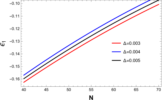
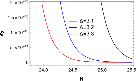
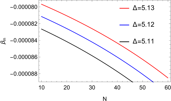
Fig.4 illustrates spectral index versus e-folding number for different values of the Barrow parameter . The latest observational data states that lies in the range [53]. In our model, the spectral index nearly lies between the above-mentioned range. We also see that for a greater value of , we get a greater value of . In Fig.5 we have plotted the tensor-to-scalar ratio against the e-folding number for different values of the Barrow parameter . From the latest observational data, it is known that the upper limit of is . From the plot, we see that for our model lies in this admissible range. It is also seen that generally, for a higher value of , we get a higher value of .
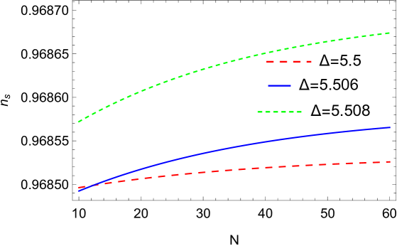
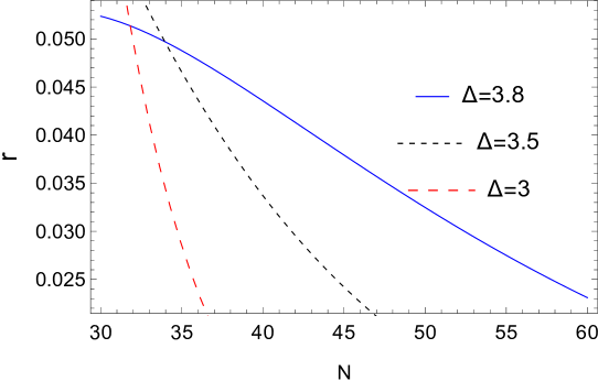
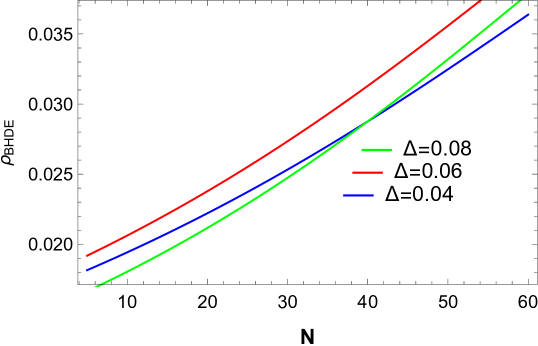
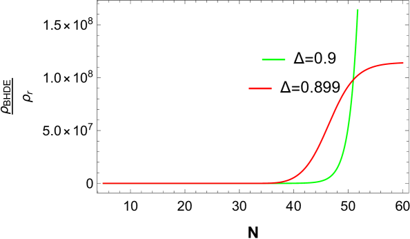
Fig.6 illustrates the behavior of energy density of BHDE for different values of the Barrow parameter. It is apparent that energy density was high during the initial time and decreased over time which is quite expected in an expanding scenario. Moreover, it shows that energy was transmitted from BHDE to radiation during the inflation. We do not get a clear comparison depending on the values of , since there is a cross-over between the trajectories. In Fig.7 the ratio of the holographic energy density and radiation density is plotted. At the initial time, the ratio was high however, at the end of the inflation the ratio decreases as the ratios come close to each other.
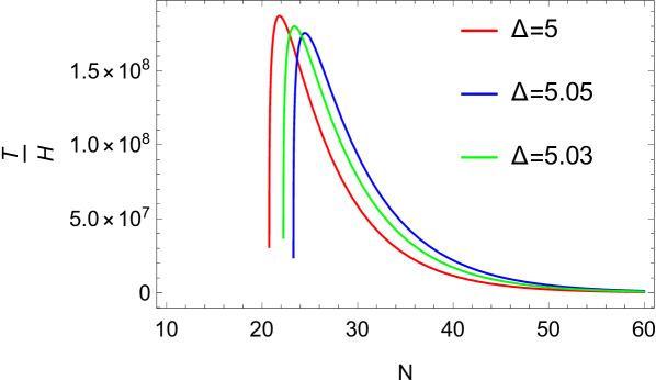
Finally, we have observed the behavior of and in Fig.8. In Fig.8 it is seen that is very much greater than 1 i.e in the presence of a thermal bath when the quantum fluctuations of the fields are dominated by the thermal fluctuations. So our model perfectly supports a warm inflationary scenario.
4 Discussion and Conclusion
Warm inflation offers a framework for comprehending the dynamics of the early universe in contrast to classical cold inflation. The inflationary paradigm is introduced to rectify the shortcomings of the traditional cosmological model. Inflationary scenarios can be classified into two categories: warm inflation and cold inflation. In cold inflation, the matter field does not interact with radiation and it slowly rolls to its flat potential. However, for the warm inflationary scenario, the inflaton interacts with other fields resulting in the transmission of energy from the inflaton to the radiation field during slow-roll. The inflaton completely decays into radiation when inflation comes to an end, preventing inflation from causing the universe to enter a very cold phase. As a result, the universe enters into radiation radiation-dominated phase without the need for a separate reheating phase.
In this article, we have studied an inflationary scenario assuming that a holographic dark fluid is the source of inflation. We have chosen Barrow holographic dark energy for this purpose in a scenario where holographic dark energy interacts with radiation and energy transmits from holographic dark energy to radiation. Here we have revised the inflationary scenario in the high dissipative regime (). Assuming this condition we have reconstructed the Hubble parameter as a function of the e-folding number . Slow roll conditions play an important role in warm inflation. A collection of slow-roll parameters determines how consistent the slow-roll approximation is. We have shown that these parameters will satisfy the warm inflationary conditions to validate our model. Moreover, after checking the tendencies of the different inflationary parameters, it was found that there is a good agreement with the observational data [53].
In a warm inflationary scenario two conditions are considered: i) thermal fluctuation dominates over quantum fluctuation i.e , ii) Holographic density dominates radiation density. We have verified these two conditions comprehensively. We have verified that for our model thermal fluctuation dominates the quantum fluctuation. Moreover, it was also confirmed that Barrow holographic energy density was high at the time of inflation, and with the evolution of the universe, the density decreased because energy was transmitted from holographic dark energy to radiation. Finally, it was seen that in the inflationary era which confirms that inflation is driven by the holographic fluid. However, the two densities come closer as inflation comes to an end. This clearly shows that the Barrow holographic dark energy model can be a novel candidate for driving warm inflation.
Acknowledgments
P.R. acknowledges the Inter-University Centre for Astronomy and Astrophysics (IUCAA), Pune, India for granting visiting associateship.
References
- [1] M.Gasperini, G. Veneziano:- Astroparticle Physics 1(3), 317 (1993).
- [2] H. Kragh:- Book chapter: Big Bang Cosmology, Book: Cosmology (pp. 371-390), CRC Press eBook ISBN: 9781003418047 (2023).
- [3] F. Mercati:- JCAP 10 025 (2019).
- [4] A. D. Linde:- Phys. Lett. B 108, 389 (1982)
- [5] A. H. Guth:- Phys. Rev. D 23 , 347 (1981).
- [6] A. D. Linde:- Phys. Lett. B 108, 389 (1982).
- [7] R. H. Brandenberger, Inflationary Cosmology: Progress and Problems, in Large Scale Structure Formation, edited by R. Mansouri and R. Brandenberger (Springer, Dordrecht), pp. 169–211 (2000)
- [8] S. W. Hawking, I. G. Moss:- Nuclear Physics B, 224(1), 180 (1983).
- [9] J. A. Vazquez, L. E. Padilla, T. Matos:- Rev. Mex. Fis. E, 17, 1 (2020).
- [10] G. Barenboim, W. H. Kinney:- JCAP 0703, 014 (2007).
- [11] M. Fairbairn, M. H. G. Tytgat:- Phys. Lett. B546, 1 (2002).
- [12] N. Nazavari, A. Mohammadi, Z. Ossoulian, K. Saaidi:- Phys. Rev. D, 93 123504 (2016).
- [13] S. Maity, P. Rudra:- JHAP 2, 1 (2022).
- [14] R. Maartens, D. Wands, B. A. Bassett, I. P. Heard:- Phys. Rev. D 62, 041301 (2000).
- [15] S. Alexander, D. Jyoti, A. Kosowsky, A. Marciano:- JCAP (05), 005 (2015 ).
- [16] A. Berera, L. Z. Fang:- Phys. Rev. Lett., 74(11), 1912 (1995).
- [17] S. Bartrum, M. Bastero-Gil, A. Berera, R. Cerezo, R. O. Ramos , J. G. Rosa:- Phys. Lett. B, 732, 116 (2014).
- [18] A. Berera:- Nuclear Physics B, 585(3), 666 (2000).
- [19] I. G. Moss:- Phys. Lett. B, 154, 120 (1985).
- [20] A Berera:- Contemporary Physics 47, 33 (2006).
- [21] R. O. Ramos, L. A. da Silva:- JCAP,1303, 032 (2013).
- [22] A. Berera, M. Gleiser , R. O. Ramos:- Phys. Rev. D, 58, 123508 (1998).
- [23] I. G. Moss, C. Xiong:- arxiv: hep-ph/0603266.
- [24] M. Bastero-Gil, A. Berera, J. G. Rosa:- Phys. Rev. D, 84, 103503 (2011).
- [25] T. Matsuda:- Phys. Rev. D, 87, 026001 (2013).
- [26] M. Bastero-Gil, A. Berera:- Int. J. Mod. Phys. A, 24, 2207 (2009).
- [27] H. Mishra, S. Mohanty, A. Nautiyal:- Phys. Lett. B, 710, 245 (2012).
- [28] M. Bastero-Gil, A. Berera, R. O. Ramos, J. G. Rosa:- Phys. Rev. Lett., 117, 151301 (2016).
- [29] A. Berera:- Universe 9(6), 272 (2023).
- [30] R. Rangarajan:- https://arxiv.org/pdf/1801.02648
- [31] W. Fischler, L. Susskind:- arxiv: hep-th/9806039
- [32] G.’t Hooft:- Dimensional Reduction in Quantum Gravity, arXiv:gr-qc/9310026.
- [33] J. D. Bekenstein:- Phys. Rev. D, 7, 2333 (1973).
- [34] A. G. Cohen, D. B. Kaplan, A. E. Nelson:- Phys. Rev. Lett. 82, 4971 (1999).
- [35] M. Li:- Phys. Lett. B 603, 1 (2004).
- [36] S. Wang, Y. Wang, M. Li:- Phys. Rept. 696 1 (2017).
- [37] H. Liu, K. Rajagopal, U. A. Wiedemann:- JHEP 03 066 (2007).
- [38] S. A. Hartnoll:- Class. Quant. Grav. 26 224002 (2009).
- [39] T. Takayanagi:- Class. Quant. Grav. 29 (2012) 153001.
- [40] A. Strominger:- JHEP 10 034 (2001).
- [41] J. D. Barrow:- Phys. Lett. B 808, 135643 (2020).
- [42] R. K. Kaul, P. Majumdar:- Phys. Rev. Lett. 84, 5255 (2000).
- [43] S. Carlip:- Class. Quant. Grav. 17, 4175 (2000).
- [44] C. Tsallis:- J. Statist. Phys. 52, 479 (1988).
- [45] G. Wilk, Z. Wlodarczyk:- Phys. Rev. Lett. 84, 2770 (2000).
- [46] C. Tsallis, L. J. L. Cirto:- Eur. Phys. J. C 73, 2487 (2013).
- [47] E. N. Saridakis:- Phys. Rev. D 102, 123525 (2020).
- [48] A. Mohammadi:- Phys. Rev. D 104, 123538 (2021).
- [49] M. Bastero-Gil, A. Berera, R. O. Ramos, J. G. Rosa:- Phys. Rev. Lett., 117(15), 151301 (2016).
- [50] A. N. Taylor, A. Berera:- Phys. Rev. D, 62(8), 083517 (2000).
- [51] M.Bastero-Gil, A. Berera, R.O.Ramos:- JCAP (07), 030 (2011)
- [52] A. Berera, J. Mabillard,M. Pieroni, R. O. Ramos, JCAP (07), 021 )(2018).
- [53] Y. Akrami, F. Arroja, M. Ashdown, et al.:- Astronomy Astrophysics, 641, A10. (2020).
- [54] A. Berera:- Phys. Rev. D 55, 3346 (1997).
- [55] L. M. Hall, I. G. Moss, A. Berera:- Phys. Rev. D 69(8), 083525 (2004).
- [56] M. Bastero-Gil, A.Berera:- Int. J. Mod. Phys. A 24(12), 2207 (2009).
- [57] G. Panotopoulos, N. Videla:- Eur. Phys. J. C. 75 525 (2015)