ACCO: Accumulate while you Communicate,
Hiding Communications in Distributed LLM Training

Abstract

Training Large Language Models (LLMs) relies heavily on distributed implementations, employing multiple GPUs to compute stochastic gradients on model replicas in parallel. However, synchronizing gradients in data parallel settings induces a communication overhead increasing with the number of distributed workers, which can impede the efficiency gains of parallelization. To address this challenge, optimization algorithms reducing inter-worker communication have emerged, such as local optimization methods used in Federated Learning. While effective in minimizing communication overhead, these methods incur significant memory costs, hindering scalability: in addition to extra momentum variables, if communications are only allowed between multiple local optimization steps, then the optimizer’s states cannot be sharded among workers. In response, we propose ACcumulate while COmmunicate (ACCO), a memory-efficient optimization algorithm tailored for distributed training of LLMs. ACCO allows to shard optimizer states across workers, overlaps gradient computations and communications to conceal communication costs, and accommodates heterogeneous hardware. Our method relies on a novel technique to mitigate the one-step delay inherent in parallel execution of gradient computations and communications, eliminating the need for warmup steps and aligning with the training dynamics of standard distributed optimization while converging faster in terms of wall-clock time. We demonstrate the effectiveness of ACCO on several LLMs training and fine-tuning tasks.

1 Introduction

Training modern Large Language Models (LLMs) with billions of parameters requires thousands of GPUs running in parallel. This is necessary to load the model and optimizer parameters in memory and reach the mini-batch size in the millions of tokens used to train them [65], relying on a distributed version of the backpropagation algorithm [29] with a gradient-based optimizer such as Adam [24] or AdamW [33]. However at this scale, the communication overhead necessary to synchronize gradients between workers in the data parallel setting can dominate the time to compute the model updates [46], and it has been estimated that it will remain the case even if models and hardware evolve [49], hindering the benefits of parallelization. Moreover, as all workers are synchronized through gradient communication, the training only proceeds at the speed of the slowest machine (straggler) [10, 38].

To alleviate this issue, distributed optimization algorithms reducing the amount of communication between workers have been developed, such as local optimization methods [61, 69] which are especially used in Federated Learning [37, 26]. These methods authorize performing multiple optimization steps locally before communicating and synchronizing the distributed workers, reducing the communication overhead. As communication rounds can last longer than a local gradient computation (see Fig. 3), they also naturally allow to hide the cost of communications in the training time by running them in parallel to several consecutive local computation steps [68, 57, 76, 63]. Moreover, on heterogeneous hardware, the number of computation steps can be tuned locally to the worker’s speed so that slow ones compute less than fast ones, maxing out workers’ usage [9, 35].

However, this comes at a drastic memory cost. Indeed, in the standard data parallel setting, most of the memory consumption of model states comes from storing the optimizer’s parameters, especially when training with mixed precision. To mitigate that, methods such as ZeRO [51] have been developed to avoid the replication of redundant optimizer states across the workers by sharding them. But these methods rely heavily on the fact that each mini-batch gradient is averaged over all the workers during the backward step. This is no longer the case with local optimization algorithms: if it were, then an averaging would happen at each step, defeating the purpose of the local method. This forces each worker to host a full copy of the optimizer’s parameters, drastically increasing the memory requirements. Moreover, to prevent local steps from reducing the accuracy of the resulting model, local methods often introduce an outer optimizer step at each communication, which comes with additional momentum terms [69, 63]. Hence, to store these variables, the latest state-of-the-art method CO2 [63] needs a memory overhead of 4 model copies compared to a standard distributed Adam, which itself uses an order of magnitude more memory than its sharded version [51]. This raises the following question:

Is it possible to design a memory-efficient optimization algorithm that hides the communication cost of distributed training of LLMs and accommodates heterogeneous hardware?

To completely hide the communication cost while being memory-efficient, making sharded optimizers compatible with the idea of overlapping gradient computations and communications seems natural. The concept of running two parallel processes is already present in the sharded optimization literature, but for a different purpose. ZeRO-Offload [55] introduces the "Delayed Parameter Update" (DPU) which allows running the optimizer on the CPU while computing and averaging gradients on the GPU. By running these processes in parallel, the gradients computed during one step are on a version of the model parameters that are no longer up to date, as they have been updated by the optimizer concurrently. In practice, this one-step staleness can hurt convergence, and the method can only be used after sufficiently many warmup steps of non-delayed optimization [55].

Contributions.

In this work, we introduce ACcumulate while COmmunicate (ACCO), a simple and memory-efficient optimization algorithm that (1) naturally allows to shard the optimizer parameters across workers, (2) overlaps gradients computations and communications, completely hiding the communication overhead while (3) maximizing GPU usage, even with heterogeneous hardware. (4) We introduce a novel method to compensate for the one-step delay induced by parallel execution of the gradient computations and communications, removing the need for warmup steps and (5) perfectly matching the training dynamic of standard distributed optimization. Moreover, our experiments across multiple LLMs training and fine-tuning tasks consistently show that ACCO allows for significant time gains. (6) We release an open-source implementation of ACCO.

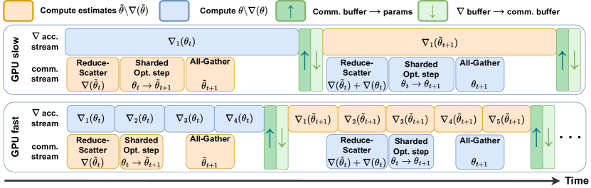
Figure 1: Overview of ACCO with a slow and a fast worker running in parallel, showing no idle time on both and completely hiding communications. The delayed update is compensated by splitting the mini-batch in two, leading to two different steps in our timeline. The first uses half of the mini-batch to estimate "next step" parameters, and the second uses the full mini-batch to update parameters.

2 Related work

Local optimization methods.

Local optimization methods allow to perform several local model updates between periodic averaging. With the SGD optimizer, these algorithms predate the deep learning era [84, 36], and their convergence properties are still investigated nowadays [81, 61, 70, 39]. Due to their practical and efficient communication scheme, they have since been used for the Distributed Training of Deep Neural Networks (DNNs) with methods such as EASGD [76], SlowMo [69] or Post-local SGD [31, 46], and are ubiquitous in Federated Learning [37, 26, 30], broadening the choice of optimizers beyond SGD [54, 22, 7]. By overlapping communications over consecutive steps of local computations, they allow to hide communication bottlenecks, resulting in algorithms such as Overlap local-SGD [68], COCO-SGD [57] or CO2 [63]. Moreover, with heterogeneous hardware, they can adapt their local computation rate to their hardware capacity [9, 35]. However this comes at the price of additional memory requirements: due to their local nature, not only do these methods prevent the use of sharded optimizers such as ZeRO [51], but they also introduce additional control variables [69, 39, 63], hindering their scalability as shown in Tab. 1. Moreover, catering for heterogeneous hardware is not straightforward, as using different numbers of local updates leads to models shifting at different speeds, requiring extra care to counter this effect [35]. On the contrary, ACCO does not lead to such disparities: it just affects how the required batch size is reached.

Overlap decentralized optimization.

The communication complexity being a core concern in decentralized optimization [74, 18], strategies have been devised to reduce communication overheads. For synchronous methods, works focus on designing algorithms with accelerated communication rates, leveraging Chebyshev polynomials [56, 28, 60]. For the asynchronous ones, they rely on the properties of the graph resistance [12, 42, 41]. Alternatively, some approaches overlap gradient and communication steps, either explicitly [3], or by modeling them with independent stochastic processes [42, 41]. However, none of these works focus on memory efficiency. Thus, they introduce additional variables and do not consider sharding the optimizer states. Moreover, they do not study optimizers other than SGD, and extending their beneficial properties to adaptive methods commonly used for DNN training such as Adam is still an ongoing research topic [2].

Memory-efficient distributed training of LLMs.

The activation memory overhead required for training Transformers [66] can be mitigated for an extra computational cost by reconstructing the input with reversible architectures [20, 34], or recomputing the activations via checkpointing [6]. Efficient LLM training also combines parallelism methods. Classical data parallelism (DP) [8] suffers both from a high communication volume and a linear increase in memory due to the model replicas. ZeRO-DP [52] and Fully-Sharded DP [79] avoid this issue by sharding the model states (i.e., the optimizer states, gradients, and parameters) between workers. This comes at the cost of further increasing the synchronization between workers and the communication volume, which can be mitigated by compression [67], memory trade-offs [77], or delayed gradients [15]. The memory can be even more reduced using expensive CPU-GPU communications to unload states on the CPU [55, 53]. On the other hand, model parallelism partitions the DNN components for parallelization, either with tensor parallelism [58] by slicing a layer’s computation on several workers, or with pipeline parallelism, which divides a model into sets of layers trained in parallel on mini-batch slices. Popularized by [19], this method leaves some workers idling and an inefficient memory overhead [13]. Allowing delay in the gradients avoids worker idleness [43, 82] but exacerbates the memory overhead, which can be partially mitigated with gradient accumulation [44, 83] and activation checkpointing [23, 32]. Combining these frameworks results in the effective 3D parallelism [59].

Delayed updates.

Delays being intrinsic to distributed asynchronous optimization, there is a rich literature studying them. In the case of distributed SGD in a parameter server setting, while early analysis showed convergence rates depending on the maximal delay [1, 62], recent lines of work improved these dependencies [25, 71, 14], proving that asynchronous SGD beats standard mini-batch SGD even with unbounded delays [38]. However, they only study plain SGD, which is hardly used for DNN training. In this context, some work focused on the interplay between SGD with momentum and delays [40, 75], while delay compensation schemes such as re-scaling updates [80, 72] or buffering them [45] were proposed for Federated Learning. But still, they only study versions of SGD and not adaptive methods commonly used for LLMs trainingsuch as Adam [24] or AdamW [33]. Closer to our work, DPU was introduced as a memory-efficient way to train LLMs by running the optimizer on the CPU while gradients are computed on the GPU [55], inducing a one-step delay between the gradients computed and the corresponding optimizer step. To mitigate it, they advise starting training by warming up for several steps with a standard method with no delay. Perhaps surprisingly, we find in our experiments that this one-step delay has a noticeable influence on the convergence of LLMs training, even when using warmup steps. Contrary to DPU, we remove the need for them, with no impact on the convergence of our training. Moreover, as it is not its purpose, DPU still runs communications in the gradient computation stream, and is thus impacted both by the communication overhead of scaling and hardware heterogeneity. Finally, in pipeline parallelism, gradient delays also affect computation, and weight prediction methods have been proposed to mitigate the effect of staleness, by predicting the future weights using the optimizer’s momentum [5]. More elaborate predictions have been proposed for SGD to further reduce the impact of the delay [27, 73].

Table 1: Comparison of characteristics and memory consumption between several methods. $\Psi$: number of parameters in the model. $N$: number of workers. $K$: memory multiplier of the optimizer (we use Adam or AdamW). For SlowMo [69] and CO2 [63], no mention of mixed precision training is made. To be fair, we assume they use it and that their additional terms are stored in half precision. While no additional momentum is required for our method, we still need a communication buffer.

Method	No comm.	Handle hetero.	Sharded	No add.	Memory consumed	$K=12,\,N=64,$
	overhead	hardware	Opt.	momentum	per worker	$\Psi=7.5$B
Baseline DDP [29]	✗	✗	✗	✓	$(2{+}2{+}K){\times}\Psi$	120 GB
ZeRO-1 [51]	✗	✗	✓	✓	$(2{+}2{+}\frac{K}{N}){\times}\Psi$	31 GB
SlowMo [69]	$\boldsymbol{\sim}$	✗	✗	✗	$(2{+}2{+}2{\times}2{+}K){\times}\Psi$	150 GB
CO2 [63]	✓	✗	✗	✗	$(2{+}2{+}4{\times}2{+}K){\times}\Psi$	180 GB
ACCO (Ours)	✓	✓	✓	✓	$(2{+}2{+}2{+}\frac{K}{N}){\times}\Psi$	46 GB

3 Method

In this section, we describe our method, including the approach to compensate for the delayed update. The algorithm will be described from the point of view of each worker $i\in\{1,...,N\}$.

Delayed Parameter Update.

First, to explain the presence of a delay, we re-purpose the "Delayed Parameter Update" (DPU) [55] to fit in our framework and match our considerations of communication overheads. Contrary to the original DPU, we run gradient communications in the same stream as the optimizer step, in parallel to the gradient computations. Moreover, to prevent the GPU $i$ from being idle at step $t$, the computations process accumulates gradients over as many mini-batches $N_{i}^{(t)}\geq 1$ as necessary until the communication process finishes, which can vary depending on the speed of the worker as shown in Fig. 1. Each worker $i$ starts from the same neural network parameters $\theta^{(0)}\in\mathbb{R}^{d}$. We denote by $F:\mathbb{R}^{d}\rightarrow\mathbb{R}$ the differentiable loss computed by our neural network. A random mini-batch (modeled through the random variable $\xi\in\Xi$ following some law $\mathcal{P}$) is drawn from the local data shard $\mathcal{D}_{i}$ to initialize the stochastic gradient ${g_{i}}^{(-1)}=\nabla F(\theta^{(0)},\xi_{i}^{(0)})$ and $N_{i}^{(-1)}=1$. Then, for $t\in[\![0,T]\!]$ we repeat the following step, with the left and right sides running in parallel:

$$g_{i}^{(t)}=\sum_{k=1}^{N_{i}^{(t)}}\nabla F(\theta^{(t)},\xi_{i,k}^{(t)})\quad,\quad\theta^{(t+1)}=\texttt{Opt}\left(\theta^{(t)},\frac{\sum_{i}g_{i}^{(t-1)}}{\sum_{i}{N_{i}}^{(t-1)}}\right)\,,$$ (DPU)

where Opt is the optimizer of our choice (e.g. Adam or AdamW for LLM training). Note that the right side does indeed combine both the gradient averaging (communications) and the optimizer step, which runs in parallel to the gradient computations to the left. Then we remark that, except at the first step $t=0$, the gradients used by Opt are computed on parameters $\theta^{(t-1)}$ which differ from $\theta^{(t)}$, the ones we apply them to. This is inherently due to the parallel nature of our execution, and what we denote by "delayed update". We will show in Sec. 5.2 that this can have drastic impacts on the convergence in practice.

Toward ACCO.

To counter this, a natural fix is to estimate what would be the parameters $\theta^{(t+2)}$ in addition to computing $\theta^{(t+1)}$. That would allow the gradients at the next round to be computed on these estimates rather than the parameters of the last step, meaning that the version of the gradients used in the Opt step would match the parameters. We denote this rule by "Weight Prediction" (WP). This time, we initialize a common $\theta^{(0)}$, $\tilde{g_{i}}^{(0)}=\nabla F(\theta^{(0)},\xi_{i}^{(0)})$, $N_{i}^{(0)}=1$ and $\tilde{\theta}^{(1)}=\texttt{Est}(\bullet)$, where Est is our estimation function that could take any argument at this point. This leads to the following:

$$\tilde{g}_{i}^{(t+1)}=\sum_{k=1}^{N_{i}^{(t+1)}}\nabla F(\tilde{\theta}^{(t+1)},\xi_{i,k}^{(t+1)})\,,\,\theta^{(t+1)}=\texttt{Opt}\left(\theta^{(t)},\frac{\sum_{i}\tilde{g}_{i}^{(t)}}{\sum_{i}{N_{i}}^{(t)}}\right)\,,\,\tilde{\theta}^{(t+2)}=\texttt{Est}(\bullet)\,.$$ (WP)

Thanks to Est, the optimizer now apply to the parameters $\theta^{(t)}$ the gradients that were computed on an estimated version $\tilde{\theta}^{(t)}$, meaning that the one-step delay has been compensated. Akin to the idea of [5] using the same SGD’s momentum several times to counter delays in pipelining, a simple estimation function could be to re-use the gradients just received and apply a second optimizer step, i.e.using $\tilde{\theta}^{(t+2)}=\texttt{Opt}\left(\theta^{(t+1)},\frac{\sum_{i}\tilde{g}_{i}^{(t)}}{\sum_{i}{N_{i}}^{(t)}}\right)$. This simple solution (denoted by ACCO-wp) is investigated in our ablations in Sec. 5.2, but we found that it leads to a training dynamic differing from the baseline, whereas ACCO, the algorithm we present next, perfectly matches it.

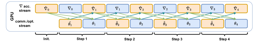
Figure 2: Illustration of ACCO’s two-stage mechanism (1)-(2) to compensate the delayed updates.

The crux of ACCO is to split the computation of the mini-batch gradients into two successive stages, where the first half of the mini-batch is used to estimate $\tilde{\theta}^{(t+1)}$ while $\theta^{(t+1)}$ is computed using the full mini-batch. This is motivated by the fact that training LLMs requires extremely large batch sizes [78], leading to the usage of gradient accumulation in most cases, and if gradients are computed sequentially on a worker, we might as well leverage this to produce our estimate. Thus, starting with an initialized $\theta^{(0)}$, $\tilde{g_{i}}^{(0)}=\nabla F(\theta^{(0)},\xi_{i}^{(0)})$ and $N_{i}^{(0)}=1$, the two stages are (left and right side running in parallel):

$${\color[rgb]{0.3203125,0.41796875,0.56640625}g_{i}^{(t)}} {\color[rgb]{0.3203125,0.41796875,0.56640625}=\sum_{k=1}^{N_{i}^{(t)}}\nabla F(\theta^{(t)},\xi_{i,k}^{(t)})} \quad,\quad{\color[rgb]{0.765625,0.5546875,0.00390625}\tilde{\theta}^{(t+1)}=\texttt{Opt}\left(\theta^{(t)},\frac{\sum_{i}\tilde{g}_{i}^{(t)}}{\sum_{i}\tilde{N_{i}}^{(t)}}\right)}\,,$$ (1)

$${\color[rgb]{0.765625,0.5546875,0.00390625}\tilde{g_{i}}^{(t+1)}} {\color[rgb]{0.765625,0.5546875,0.00390625}=\sum_{k=1}^{\tilde{N_{i}}^{(t)}}\nabla F(\tilde{\theta}^{(t+1)},\tilde{\xi}_{i,k}^{(t+1)})} \quad,\quad{\color[rgb]{0.3203125,0.41796875,0.56640625}\theta^{(t+1)}=\texttt{Opt}\left(\theta^{(t)},\frac{\sum_{i}g_{i}^{(t)}+\tilde{g}_{i}^{(t)}}{\sum_{i}N_{i}^{(t)}+\tilde{N_{i}}^{(t)}}\right)}\,.$$ (2)

We describe the different components of our two-stage mechanism as follows:

• The gradient computation stream uses the second half of the mini-batch to compute the gradients $g_{i}^{(t)}$ with respect to parameters $\theta^{(t)}$ while the communication stream estimates what would be the next steps parameters $\tilde{\theta}^{(t+1)}$ using the estimated gradients $\tilde{g}_{i}^{(t)}$.

• The computation stream uses the first half of the mini-batch to estimate what would be the gradients $\tilde{g}_{i}^{(t+1)}$ of the next parameters $\theta^{(t+1)}$ using estimated parameters $\tilde{\theta}^{(t+1)}$ while the communication stream computes $\theta^{(t+1)}$ using the full mini-batch. Note that it starts from the same version of the parameters $\theta^{(t)}$ as in step (1). The first half $\tilde{g}_{i}^{(t)}$ was estimated at step (2) of the last round, while the second half $g_{i}^{(t)}$ was just computed in (1).

As illustrated in Fig. 2, by splitting the computations of the mini-batch gradients into two halves, we do allow the gradient computations and communications timelines to run in parallel while performing ACCO’s weight prediction estimation to compensate for the delayed update.

4 Empirical motivation and cluster setting

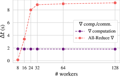
Figure 3: Time (per worker) spent computing and averaging gradients of a Llama-2 7B model for different numbers of GPUs.

In this section, we empirically motivate the need for methods mitigating communication overhead in Distributed Data Parallel (DDP) [29]. Our goal is to illustrate that the time spent communicating gradients can quickly trump the one used for computing them when using DDP to train LLMs. For that, we measure the time necessary to perform a forward and backward pass on a Llama-2 model [65] with 7B parameters hosted on a single GPU, using a batch size maxing out its memory. We compare this to the time necessary to compute an All-Reduce on those gradients with the NCCL backend, varying the number of distributed workers. On all the following, we experiment on our local cluster of NVIDIA A100-80GB GPUs with 8 GPUs per node and an Omni-PAth interconnection network at 100 Gb/s for inter-node connections, intra-node connections being done with NVLink 300 GB/s. Each distributed worker is hosted on a single GPU. We observe in Fig. 3 that when we communicate outside of a GPU node in our cluster, the time needed to average the gradients across workers can take more than four times the one spent on the whole forward and backward step. As DDP only partially hides communications during the backward [29], this means that our GPUs remain idle the majority of the time when we use more than 24 distributed workers, motivating the need for methods leveraging this time to compute instead.

5 Experiments

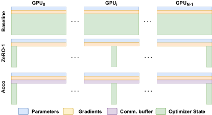
Figure 4: Memory requirements of ACCO  vs DDP and ZeRO-1, see Tab.1 for quantitative details.

In this section, we lay down our experiments. First in Sec. 5.1, we detail the common setup for all our experiments. Second, in Sec. 5.2, we illustrate the failings of DPU and ACCO-wp that we hinted at in Sec. 3, which led us to crafting ACCO. For this first exploration, we focus on small language models and datasets, using TinyStories [11] as our test-bed. Then in Sec. 5.3, we verify that ACCO allows to efficiently train LLMs at scale by considering a 125M parameters GPT-Neo architecture [4] and the OpenWebText dataset [17].Finally in Sec. 5.4, we consider even larger models by using ACCO for an instruction fine-tuning task with a 2.7B parameters GPT-Neo, which accentuates the effects of the inter-node communication bottlenecks and highlights all the more the benefits of our method. They are further displayed in Appendix C where we compare between ACCO and DDP on heterogeneous hardware. Our method allows faster GPUs to accumulate while they wait for the slowest worker instead of remaining idle as in DDP, thus allowing us to compute gradients for large batch sizes faster than the baseline, resulting in quicker convergence in wall-clock time.

5.1 Experimental setup

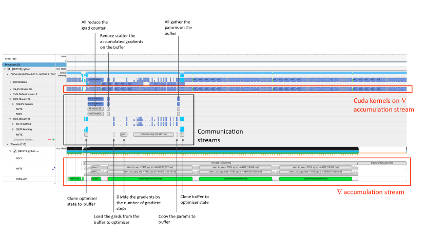
Figure 9: Nsight system profile of our implementation of ACCO: our two steams do run in parallel. In this Figure, the computation take more time than the communication because we only profiled small scale experiments with 8 workers, and small number of parameters (36M as we profiled on our TinyStories [11] setting). This changes when using larger models and more workers, as seen in 4.

All of our experiments are performed on the GPU cluster described in Sec. 4. A detailed pseudo-code for ACCO can be found in Appendix A.2. Our implementation is in Pytorch [48], and we verified that our code for ACCO does indeed produces two different CUDA streams running in parallel for the computations and communications using NVIDIA’s Nsight System to profile it, as shown in Fig. 9 in the Appendix. We trained all our models with AdamW [33], using mixed precision: our model parameters, gradient accumulation buffer, and communication buffers are in bfloat16 [21] while our sharded optimizer states are in single precision, as shown in Fig. 4. We compared our algorithm ACCO to several baselines in different settings, including Pytorch’s Distributed Data Parallel (DDP) method [29] with ZeRO-1 [51].

5.2 Crafting ACCO on TinyStories

Here, we experiment with small language models on the TinyStories dataset [11], following the configuration and training hyper-parameters of their paper [11] to the best of our abilities. Hence, we use a 36M parameters GPT-Neo based [4] decoder-only transformer architecture. To match the 10k vocabulary they used, we trained our own BPE tokenizer on the TinyStories dataset. For our experiments, we used up to 8 workers on a single node.

Impact of delayed updates.

First, we investigate the impact of using delayed updates, re-purposing DPU [55] as described in Sec. 3. We run three variants of this algorithm: (1) with no warmup, (2) with 40 warmup steps of non-delayed optimization step before switching to DPU (recommended recipe in [55]), and (3) with 500 steps of warmup. We report in Fig. 5 our training losses on 8 distributed workers averaged over $3$ runs.

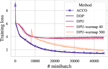
(a) Training with the specified amount in [11].

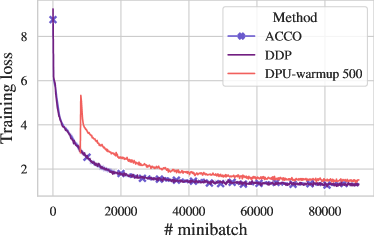
(b) Training for twice the specified amount.

Figure 5: Impact of the delayed update and the amount of warmup steps on the training

We remark that using delayed updates can greatly hurt convergence, especially when no or too few warmup steps are performed. Surprisingly, the number of warmup steps given in [55] does not work here, hinting that it is a sensitive hyper-parameter to tune for each use-case. When sufficiently many warmup steps are done, first the training loss follows exactly the baseline one, but immediately spikes as soon as the delay is introduced. If we train for twice as long than specified in [11], then the DPU training curve approaches the baseline one, without totally catching it. Contrary to this, the training curve of our algorithm ACCO perfectly matches DDP’s one from the beginning.

A simple approach to compensate delays.

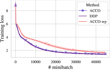
Figure 6: Comparison of ACCO with its Weight Prediction version on TinyStories.

After noticing the detrimental impact of using delayed updates on the training performances of our models, we test our first approach to mitigate it. For that, we implement ACCO-wp, the Weight Prediction method described in Sec. 3. This method applies two consecutive optimizer steps, re-using the same mini-batch of gradients twice. The first step produces the usual updated parameters, and the second one is used to predict the parameters of the next step so that gradients can be computed on this estimate rather than on a stale version of the model. In Fig. 6 we compare the training curves of this delay-compensation method to ours. We remark that, while ACCO perfectly matches the DDP baseline at all times, ACCO-wp displays worse behavior, especially at the beginning of the training. Thus, we dismiss this method and keep ours for the remaining of the experiments.

5.3 Passing the scaling test: training GPT-Neo on OpenWebText

Table 2: Perplexity of our trained LLMs

Method	LAMBADA (ppl $\downarrow$)	OpenWebText (ppl $\downarrow$)
ACCO 1x8	47.1	24.2
DDP 1x8	47.5	24.3
ACCO 4x8	45.5	22.5
DDP 4x8	44.1	21.7

To assess how ACCO scales with larger models and more data, we pre-trained a model equivalent to GPT-2 [50] with both ACCO and DDP. Specifically, we used the GPT-Neo architecture [4] with 125 million parameters and the OpenWebText dataset [17], which contains 40 GB of text. We used the GPT-Neo tokenizer, pre-trained on the Pile dataset [16]. The models were trained on sequences of 1024 tokens, with documents concatenated using end-of-sequence tokens. To assess the impact of using different hardware, the experiment was repeated on 2 different clusters. The first was conducted on 8 H100-PCIe 80GB on a single node. The second was on 32 A100-80G GPU distributed on 4 nodes. We maxed out the memory of our GPUs with a local mini-batch size of 24. To reach a sufficiently large overall batch size, we used 1 step of gradient accumulation for DDP, and none for ACCO as our method naturally accumulates over 1 step, resulting for the first and second experiments in respectively 400K and 1.5M tokens per effective batch for both ACCO and DDP. In Tab. 3, we report additional experimental details, and notice that training with ACCO allows for significant time gains, which is additionally illustrated in Fig. 7. Moreover, to prevent GPUs from idling while waiting for communications, ACCO adaptively scheduled 315 supplementary accumulation steps over the whole training. Further details and results for the H100 experiment can be found in Appendix B.

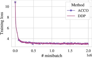
(a) Evolution of the loss over the whole training.

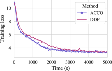
(b) Focus on the first part of the training w.r.t time.

Figure 7: Training curves for ACCO and DDP with 32 workers trained for 50B tokens.

Tab. 2 reports the perplexity of trained language models with both methods, which is a commonly used metric to evaluate pre-trained language models, as it quantifies the uncertainty of a model at predicting the next token. We evaluate the perplexity of language models on LAMBADA [47] and a test split of OpenWebText, and report similar results for both methods.

5.4 Advantages of using ACCO for instruction fine-tuning

In previous sections, we compared ACCO  against DDP in the pre-training stage. To further validate our algorithm, we additionally fine-tuned a pre-trained model on supervised instruction data. We consider the GPT-Neo 2.7B model [4] pre-trained on the Pile dataset [16] and finetuned it on the Alpaca dataset [64] containing 52k pairs of instruction/answer. We fine-tuned the model using two configurations: 8 A100-80G on a single node, and 8 A100-80G distributed equally across 2 nodes. Samples are padded to match the longest sequence in the mini-batch. We fixed the mini-batch size at 4, leading to a total batch size of 128 for all methods. For DDP and DPU, we used a gradient accumulation of 4, while for ACCO , a gradient accumulation of 2 to account for the ACCO  accumulation described in Sec. 1. The learning rate was set to $2\times 10^{-5}$ for all methods with a warmup of 50 steps, for DPU.

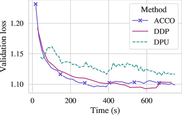
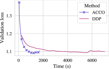
Figure 8: Validation curve with 8 workers on 1 node (left), and 4 workers/node on 2 nodes (right).

In this setting, padding to the longest sequence in the mini-batch induces more variability in the number of tokens per mini-batch. This results in more variability in the computational load for each worker, leading to increased wait times for synchronization. We observe in Fig. 8 that ACCO hits a lower validation loss faster than DDP on both 1 node and 2 nodes settings. Note that the difference between ACCO and DDP is accentuated when workers are distributed on multiple nodes. In 11, we observe that ACCO is less data efficient at the beginning of training, as evidenced by a higher loss compared to DDP for the same number of seen tokens. This is likely due to the fact that ACCO favors using tokens to increase the batch size to hide communication delays, meaning that fewer optimizer steps are performed per token compared to DDP. However, both algorithms converge to very similar loss values by the end of the training.

Table 3: Pre-training and finetuning time speedup with ACCO  against DDP on various setups.

Stage	Model	GPUs	#tokens	DDP	ACCO	($\Delta T$)
Pre-training	GPT-Neo-125M	1x8	6B	4h41min	4h25min	($-5.69\%$)
		4x8	50B	14h41min	10h55min	($-25.65\%$)
Finetuning	GPT-Neo-2.7B	1x8	80M	43min	25min	($-41.86\%$)
		2x4	80M	3h46min	29min	($-87.17\%$)

6 Limitations

Experiments mainly on one cluster environment.

Due to the lack of variety in the compute environments we have access to, the majority of our experiments were performed on a single cluster, described in Sec. 4. This is a communication-constrained setting, as our hardware is not the most cutting-edge in that regard as discussed in Sec. 4. This particularly flatters our method in comparison to DDP, as it accentuates the impact of the communication overhead in the wall clock time. However, to mitigate this one-sidedness, we also run a small pre-training study on one of the fastest hardware available today, and report in Tab. 3 that even in that case, ACCO leads to a 5% time gain.

Communication cost only hidden, not reduced.

While local optimization methods tackle the communication overhead problem with scarce communications, here we only hide them. Thus, our method does not lead to energy savings, nor question the cost of highly synchronized infrastructure. However, ACCO naturally maximizes the hardware throughput, allowing to reduce their use time.

Further memory savings avenue not explored.

Due to the parallel nature of ACCO, removing the reliance on communication and gradient buffers seems hardly possible, questioning the feasibility of further memory savings if all executions are kept on the GPU. But, akin to ZeRO-Offload [55], the communication and optimizer stream could entirely be run on CPU, which would allow significant memory gains. We did not experiment with this idea, and let this consideration for future work.

Conclusion

We propose ACCO, a novel algorithm that addresses the memory and communication challenges inherent in training LLMs on distributed systems. By allowing for parallel computation and communication of gradients while permitting sharding the optimizer states, ACCO  effectively reduces communication overhead in a memory-efficient fashion. We introduce a novel two-stage mechanism to compensate for the delayed update inherent to this parallel setting, which ensures consistent convergence dynamics with the standard optimization algorithm for large-scale distributed LLM training without the need for warmup steps. We empirically confirm the benefits of our methods over several pre-training and finetuning tasks, reporting drastically reduced training times compared to our baseline, especially in multi-node settings or with heterogeneous devices.

Appendix

Appendix A Implementation Details

A.1 Profiling Results

A.2 Algorithm presentation

Algorithm 1 Training with ACCO  in parallel for a worker $i$

1:  Input: Model with differentiable loss $F$, number of models $N$, initial parameters $\theta^{(0)}$, training steps $T$, dataset shards $\mathcal{D}_{i}$.

2:  Initialize: gradients ${g_{i}}^{(-1)}=\nabla F(\theta^{(0)},\xi_{i}^{(0)})$ and number of gradients $N_{i}^{(-1)}=1$

3:   # Computation CUDA stream

4:  while  $t<T$ do

5:      Stage 1.

6:     while  not Ready_for_Stage_2  do

7:         $\xi_{i}^{(t)}\leftarrow\mathcal{D}_{i}$

8:         $g_{i}^{(t)}\leftarrow g_{i}^{(t)}+\nabla F(\theta^{(t)},\xi_{i}^{(t)})$

9:         $N_{i}^{(t)}\leftarrow N_{i}^{(t)}+1$

10:      $\tilde{\theta}^{(t+1)}\leftarrow\textbf{Buffer}_{i}$

11:      $\textbf{Buffer}_{i}\leftarrow(N_{i}^{(t)},g_{i}^{(t)})$

12:      Stage 2.

13:     while  not Ready_for_Stage_1  do

14:         $\xi_{i}^{(t)}\leftarrow\mathcal{D}_{i}$

15:         $\tilde{g}_{i}^{(t)}\leftarrow\tilde{g}_{i}^{(t)}+\nabla F(\tilde{\theta}^{(t+1)},\xi_{i}^{(t)})$

16:         $\tilde{N}_{i}^{(t)}\leftarrow\tilde{N}_{i}^{(t)}+1$

17:         $t\leftarrow t+1$

18:      $\theta^{(t+1)}\leftarrow\textbf{Buffer}_{i}$

19:      $\textbf{Buffer}_{i}\leftarrow(\tilde{N}_{i}^{(t)},\tilde{g}_{i}^{(t)})$

20:  

21:   # Communication CUDA stream

22:  while True do

23:      Stage 1.

24:      $(\tilde{N}_{i}^{(t)},\tilde{g}_{i}^{(t)})\leftarrow\textbf{Buffer}_{i}$

25:      $\sum_{i}\tilde{N}_{i}^{(t)}\leftarrow\texttt{All\_Reduce}(\tilde{N}_{i}^{(t)})$

26:      $\texttt{Shard}_{i}\left(\sum_{i}g_{i}^{(t)}\right)\leftarrow\texttt{Reduce\_Scatter}(\tilde{g}_{i}^{(t)})$

27:      $\texttt{Shard}_{i}\left(\tilde{\theta}^{(t+1)}\right)\leftarrow\texttt{ShardedOpt}\left(\texttt{Shard}_{i}\left(\theta^{(t)}\right),\texttt{Shard}_{i}\left(\frac{\sum_{i}\tilde{g}_{i}^{(t)}}{\sum_{i}\tilde{N_{i}}^{(t)}}\right)\right)$

28:      $\textbf{Buffer}_{i}\leftarrow\texttt{All\_Gather}(\texttt{Shard}_{i}\left(\tilde{\theta}^{(t+1)}\right))$

29:      $N_{i}^{(t)}\leftarrow 0$

30:      $\texttt{Ready\_for\_Stage\_2}\leftarrow\textbf{True}$

31:      $\texttt{Ready\_for\_Stage\_1}\leftarrow\textbf{False}$

32:      Stage 2.

33:      $(N_{i}^{(t)},g_{i}^{(t)})\leftarrow\textbf{Buffer}_{i}$

34:      $\sum_{i}N_{i}^{(t)}+\tilde{N}_{i}^{(t)}\leftarrow\texttt{All\_Reduce}(N_{i}^{(t)}+\sum_{i}\tilde{N}_{i}^{(t)})$

35:      $\texttt{Shard}_{i}\left(\sum_{i}g_{i}^{(t)}+\tilde{g}_{i}^{(t)}\right)\leftarrow\texttt{Reduce\_Scatter}(g_{i}^{(t)}+\sum_{i}\tilde{g}_{i}^{(t)})$

36:      $\texttt{Shard}_{i}\left(\theta^{(t+1)}\right)\leftarrow\texttt{ShardedOpt}\left(\texttt{Shard}_{i}\left(\theta^{(t)}\right),\texttt{Shard}_{i}\left(\frac{\sum_{i}g_{i}^{(t)}+\tilde{g}_{i}^{(t)}}{\sum_{i}N_{i}^{(t)}+\tilde{N_{i}}^{(t)}}\right)\right)$

37:      $\textbf{Buffer}_{i}\leftarrow\texttt{All\_Gather}(\texttt{Shard}_{i}\left(\theta^{(t+1)}\right))$

38:      $\tilde{N}_{i}^{(t)}\leftarrow 0$

39:      $\texttt{Ready\_for\_Stage\_1}\leftarrow\textbf{True}$

40:      $\texttt{Ready\_for\_Stage\_2}\leftarrow\textbf{False}$

Appendix B Experimental Details and Further Results

B.1 Pre-training on TinyStories

For experiements in section 5.2, we used the configuration of We used the dataset TinyStories available on the Huggingface Hub . We trained our own 10k vocabulary tokenizer on the dataset.

B.2 Pre-training on OpenWebText

For all pre-training experiments on OpenWebText, the configuration used to instantiate the GPTNeo 125M is available on the Huggingface Hub. We only changed the "max_position_embeddings" parameter from 2048 to 1024. We used the OpenWebText dataset available on Huggingface. We also report in Fig. 10 further results for the pre-training on H100 GPUs.

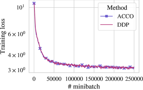
Figure 10: Training loss during training on OpenWebText with 8 H100 GPUs and 6B tokens.

Table 4: Training hyperparameters for ACCO and DDP configurations.

Hyperparameter	8 H100	32 A100
mini-batch_size	24	24
n_grad_accumulation	ACCO: - DDP: 1	ACCO: - DDP: 1
sequence_len	1024	1024
#tokens_batch	400K	1.5M
optimizer	AdamW	AdamW
learning_rate	6e-4	6e-4
weight_decay	0.1	0.1
adam_beta1	0.9	0.9
adam_beta2	0.95	0.95
nb_steps_tot	50000	50000
scheduler	cosine	cosine
n_warmup_steps	0	0

B.3 Instruction Fine-Tuning

For all fine-tuning experiments, we used the pre-trained GPT-neo 2.7B available on the Huggingface Hub and the associated tokenizer. We used the Alpaca dataset available on Huggingface.

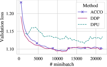
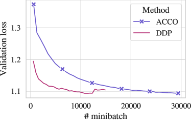
Figure 11: Validation curve with 8 workers on a single node (left), and with 4 workers per nodes on 2 nodes (right).

Table 5: Finetuning hyperparameters for ACCO, DDP and DPU configurations.

Hyperparameter	ACCO	DDP	DPU
mini-batch_size	4	4	4
n_grad_accumulation	2	4	4
total batch_size	128	128	128
optimizer	AdamW	AdamW	AdamW
learning_rate	2e-5	2e-5	2e-5
weight_decay	0.0	0.0	0.0
adam_beta1	0.9	0.9	0.9
adam_beta2	0.95	0.95	0.95
nb_steps_tot	50000	50000	50000
scheduler	cosine	cosine	cosine
n_warmup_steps	0	0	50

Appendix C Experiment Using Heterogeneous Devices

To witness the impact of using heterogeneous devices, we run our algorithm ACCO and compared it to the DDP baseline in a four workers setting, with one of the GPU four times slower than the other three, as shown in Fig. 12. As we experiment on a cluster of A100 GPUs, we simulated the heterogeneity of the hardware by using the time.sleep() python command. First, we measured the time that a standard forward-backward step takes in our homogeneous cluster, and put to sleep one of the four GPUs for three times this amount after each forward-backward pass. In this context, DDP is only as fast as the slowest worker, meaning that 3 of the 4 workers are idle a third of the time. With our method, the other workers accumulate during the time they are waiting for the slow one to finish. This means that ACCO  allows to compute gradients for large batch sizes faster than standard baselines, resulting in faster convergence in terms of wall-clock time, as displayed in Fig. 12.

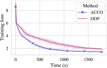
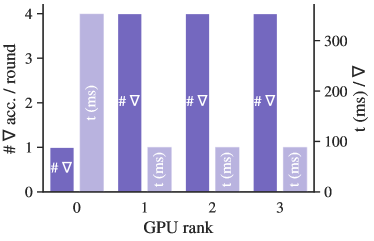
Figure 12: Training curves with 3 normal workers and 1 slow worker ($4\times$ slower).

References

- [1] A. Agarwal and J. C. Duchi. Distributed delayed stochastic optimization. In J. Shawe-Taylor, R. Zemel, P. Bartlett, F. Pereira, and K. Weinberger, editors, Advances in Neural Information Processing Systems, volume 24. Curran Associates, Inc., 2011.
- [2] B. M. Assran, A. Aytekin, H. R. Feyzmahdavian, M. Johansson, and M. G. Rabbat. Advances in asynchronous parallel and distributed optimization. Proceedings of the IEEE, 108(11):2013–2031, 2020.
- [3] M. Assran, N. Loizou, N. Ballas, and M. Rabbat. Stochastic gradient push for distributed deep learning. In K. Chaudhuri and R. Salakhutdinov, editors, Proceedings of the 36th International Conference on Machine Learning, volume 97 of Proceedings of Machine Learning Research, pages 344–353. PMLR, 09–15 Jun 2019.
- [4] S. Black, G. Leo, P. Wang, C. Leahy, and S. Biderman. GPT-Neo: Large Scale Autoregressive Language Modeling with Mesh-Tensorflow, Mar. 2021.
- [5] C.-C. Chen, C.-L. Yang, and H.-Y. Cheng. Efficient and robust parallel dnn training through model parallelism on multi-gpu platform, 2019.
- [6] T. Chen, B. Xu, C. Zhang, and C. Guestrin. Training deep nets with sublinear memory cost, 2016.
- [7] X. Chen, X. Li, and P. Li. Toward communication efficient adaptive gradient method. Proceedings of the 2020 ACM-IMS on Foundations of Data Science Conference, 2020.
- [8] J. Dean, G. Corrado, R. Monga, K. Chen, M. Devin, M. Mao, M. a. Ranzato, A. Senior, P. Tucker, K. Yang, Q. Le, and A. Ng. Large scale distributed deep networks. In F. Pereira, C. Burges, L. Bottou, and K. Weinberger, editors, Advances in Neural Information Processing Systems, volume 25. Curran Associates, Inc., 2012.
- [9] M. Diskin, A. Bukhtiyarov, M. Ryabinin, L. Saulnier, Q. Lhoest, A. Sinitsin, D. Popov, D. Pyrkin, M. Kashirin, A. Borzunov, A. V. del Moral, D. Mazur, I. Kobelev, Y. Jernite, T. Wolf, and G. Pekhimenko. Distributed deep learning in open collaborations. In A. Beygelzimer, Y. Dauphin, P. Liang, and J. W. Vaughan, editors, Advances in Neural Information Processing Systems, 2021.
- [10] S. Dutta, J. Wang, and G. Joshi. Slow and stale gradients can win the race. IEEE Journal on Selected Areas in Information Theory, 2(3):1012–1024, 2021.
- [11] R. Eldan and Y. Li. Tinystories: How small can language models be and still speak coherent english?, 2023.
- [12] M. Even, R. Berthier, F. Bach, N. Flammarion, H. Hendrikx, P. Gaillard, L. Massoulié, and A. Taylor. A continuized view on nesterov acceleration for stochastic gradient descent and randomized gossip. In A. Beygelzimer, Y. Dauphin, P. Liang, and J. W. Vaughan, editors, Advances in Neural Information Processing Systems, 2021.
- [13] S. Fan, Y. Rong, C. Meng, Z. Cao, S. Wang, Z. Zheng, C. Wu, G. Long, J. Yang, L. Xia, et al. Dapple: A pipelined data parallel approach for training large models. In Proceedings of the 26th ACM SIGPLAN Symposium on Principles and Practice of Parallel Programming, pages 431–445, 2021.
- [14] H. R. Feyzmahdavian and M. Johansson. Asynchronous iterations in optimization: New sequence results and sharper algorithmic guarantees. Journal of Machine Learning Research, 24(158):1–75, 2023.
- [15] L. Fournier and E. Oyallon. Cyclic data parallelism for efficient parallelism of deep neural networks, 2024.
- [16] L. Gao, S. Biderman, S. Black, L. Golding, T. Hoppe, C. Foster, J. Phang, H. He, A. Thite, N. Nabeshima, et al. The pile: An 800gb dataset of diverse text for language modeling. arXiv preprint arXiv:2101.00027, 2020.
- [17] A. Gokaslan, V. Cohen, E. Pavlick, and S. Tellex. Openwebtext corpus. http://Skylion007.github.io/OpenWebTextCorpus, 2019.
- [18] E. Gorbunov, A. Rogozin, A. Beznosikov, D. Dvinskikh, and A. Gasnikov. Recent Theoretical Advances in Decentralized Distributed Convex Optimization, pages 253–325. Springer International Publishing, Cham, 2022.
- [19] Y. Huang, Y. Cheng, A. Bapna, O. Firat, D. Chen, M. Chen, H. Lee, J. Ngiam, Q. V. Le, Y. Wu, et al. Gpipe: Efficient training of giant neural networks using pipeline parallelism. Advances in neural information processing systems, 32, 2019.
- [20] J.-H. Jacobsen, A. W. Smeulders, and E. Oyallon. i-revnet: Deep invertible networks. In International Conference on Learning Representations, 2018.
- [21] D. Kalamkar, D. Mudigere, N. Mellempudi, D. Das, K. Banerjee, S. Avancha, D. T. Vooturi, N. Jammalamadaka, J. Huang, H. Yuen, J. Yang, J. Park, A. Heinecke, E. Georganas, S. Srinivasan, A. Kundu, M. Smelyanskiy, B. Kaul, and P. Dubey. A study of bfloat16 for deep learning training, 2019.
- [22] S. P. Karimireddy, M. Jaggi, S. Kale, M. Mohri, S. J. Reddi, S. U. Stich, and A. T. Suresh. Mime: Mimicking centralized stochastic algorithms in federated learning. ArXiv, abs/2008.03606, 2020.
- [23] C. Kim, H. Lee, M. Jeong, W. Baek, B. Yoon, I. Kim, S. Lim, and S. Kim. torchgpipe: On-the-fly pipeline parallelism for training giant models, 2020.
- [24] D. Kingma and J. Ba. Adam: A method for stochastic optimization. In International Conference on Learning Representations (ICLR), San Diega, CA, USA, 2015.
- [25] A. Koloskova, S. U. Stich, and M. Jaggi. Sharper convergence guarantees for asynchronous sgd for distributed and federated learning. In Proceedings of the 36th International Conference on Neural Information Processing Systems, NIPS ’22, Red Hook, NY, USA, 2024. Curran Associates Inc.
- [26] J. Konecný, H. B. McMahan, D. Ramage, and P. Richtárik. Federated optimization: Distributed machine learning for on-device intelligence. ArXiv, abs/1610.02527, 2016.
- [27] A. Kosson, V. Chiley, A. Venigalla, J. Hestness, and U. Köster. Pipelined backpropagation at scale: Training large models without batches, 2021.
- [28] D. Kovalev, A. Salim, and P. Richtarik. Optimal and practical algorithms for smooth and strongly convex decentralized optimization. In H. Larochelle, M. Ranzato, R. Hadsell, M. Balcan, and H. Lin, editors, Advances in Neural Information Processing Systems, volume 33, pages 18342–18352. Curran Associates, Inc., 2020.
- [29] S. Li, Y. Zhao, R. Varma, O. Salpekar, P. Noordhuis, T. Li, A. Paszke, J. Smith, B. Vaughan, P. Damania, and S. Chintala. Pytorch distributed: experiences on accelerating data parallel training. Proc. VLDB Endow., 13(12):3005–3018, aug 2020.
- [30] T. Li, A. K. Sahu, M. Zaheer, M. Sanjabi, A. Talwalkar, and V. Smith. Federated optimization for heterogeneous networks. In ICML Workshop on Adaptive & Multitask Learning: Algorithms & Systems, 2019.
- [31] T. Lin, S. U. Stich, K. K. Patel, and M. Jaggi. Don’t use large mini-batches, use local sgd. In International Conference on Learning Representations, 2020.
- [32] Y. Liu, S. Li, J. Fang, Y. Shao, B. Yao, and Y. You. Colossal-auto: Unified automation of parallelization and activation checkpoint for large-scale models, 2023.
- [33] I. Loshchilov and F. Hutter. Decoupled weight decay regularization. In International Conference on Learning Representations, 2019.
- [34] K. Mangalam, H. Fan, Y. Li, C.-Y. Wu, B. Xiong, C. Feichtenhofer, and J. Malik. Reversible vision transformers. In Proceedings of the IEEE/CVF Conference on Computer Vision and Pattern Recognition, pages 10830–10840, 2022.
- [35] A. Maranjyan, M. Safaryan, and P. Richtárik. Gradskip: Communication-accelerated local gradient methods with better computational complexity, 2022.
- [36] R. McDonald, K. Hall, and G. Mann. Distributed training strategies for the structured perceptron. In Human Language Technologies: The 2010 Annual Conference of the North American Chapter of the Association for Computational Linguistics, HLT ’10, page 456–464, USA, 2010. Association for Computational Linguistics.
- [37] B. McMahan, E. Moore, D. Ramage, S. Hampson, and B. A. y. Arcas. Communication-Efficient Learning of Deep Networks from Decentralized Data. In A. Singh and J. Zhu, editors, Proceedings of the 20th International Conference on Artificial Intelligence and Statistics, volume 54 of Proceedings of Machine Learning Research, pages 1273–1282. PMLR, 20–22 Apr 2017.
- [38] K. Mishchenko, F. Bach, M. Even, and B. Woodworth. Asynchronous SGD beats minibatch SGD under arbitrary delays. In A. H. Oh, A. Agarwal, D. Belgrave, and K. Cho, editors, Advances in Neural Information Processing Systems, 2022.
- [39] K. Mishchenko, G. Malinovsky, S. Stich, and P. Richtárik. Proxskip: Yes! local gradient steps provably lead to communication acceleration! finally! arXiv preprint arXiv:2202.09357, 2022.
- [40] I. Mitliagkas, C. Zhang, S. Hadjis, and C. Ré. Asynchrony begets momentum, with an application to deep learning. In 2016 54th Annual Allerton Conference on Communication, Control, and Computing (Allerton), page 997–1004. IEEE Press, 2016.
- [41] A. Nabli, E. Belilovsky, and E. Oyallon. $\textbf{A}^2\textbf{CiD}^2$: Accelerating asynchronous communication in decentralized deep learning. In Thirty-seventh Conference on Neural Information Processing Systems, 2023.
- [42] A. Nabli and E. Oyallon. DADAO: Decoupled accelerated decentralized asynchronous optimization. In A. Krause, E. Brunskill, K. Cho, B. Engelhardt, S. Sabato, and J. Scarlett, editors, Proceedings of the 40th International Conference on Machine Learning, volume 202 of Proceedings of Machine Learning Research, pages 25604–25626. PMLR, 23–29 Jul 2023.
- [43] D. Narayanan, A. Harlap, A. Phanishayee, V. Seshadri, N. R. Devanur, G. R. Ganger, P. B. Gibbons, and M. Zaharia. Pipedream: Generalized pipeline parallelism for dnn training. In Proceedings of the 27th ACM Symposium on Operating Systems Principles, pages 1–15, 2019.
- [44] D. Narayanan, A. Phanishayee, K. Shi, X. Chen, and M. Zaharia. Memory-efficient pipeline-parallel dnn training. In International Conference on Machine Learning, pages 7937–7947. PMLR, 2021.
- [45] J. Nguyen, K. Malik, H. Zhan, A. Yousefpour, M. Rabbat, M. Malek, and D. Huba. Federated learning with buffered asynchronous aggregation. In G. Camps-Valls, F. J. R. Ruiz, and I. Valera, editors, Proceedings of The 25th International Conference on Artificial Intelligence and Statistics, volume 151 of Proceedings of Machine Learning Research, pages 3581–3607. PMLR, 28–30 Mar 2022.
- [46] J. J. G. Ortiz, J. Frankle, M. Rabbat, A. Morcos, and N. Ballas. Trade-offs of local sgd at scale: An empirical study. In NeurIPS 2020 OptML Workshop, 2021.
- [47] D. Paperno, G. Kruszewski, A. Lazaridou, N. Q. Pham, R. Bernardi, S. Pezzelle, M. Baroni, G. Boleda, and R. Fernandez. The LAMBADA dataset: Word prediction requiring a broad discourse context. In Proceedings of the 54th Annual Meeting of the Association for Computational Linguistics (Volume 1: Long Papers), pages 1525–1534, Berlin, Germany, August 2016. Association for Computational Linguistics.
- [48] A. Paszke, S. Gross, F. Massa, A. Lerer, J. Bradbury, G. Chanan, T. Killeen, Z. Lin, N. Gimelshein, L. Antiga, A. Desmaison, A. Köpf, E. Yang, Z. DeVito, M. Raison, A. Tejani, S. Chilamkurthy, B. Steiner, L. Fang, J. Bai, and S. Chintala. Pytorch: an imperative style, high-performance deep learning library. In Proceedings of the 33rd International Conference on Neural Information Processing Systems, Red Hook, NY, USA, 2019. Curran Associates Inc.
- [49] S. Pati, S. Aga, M. Islam, N. Jayasena, and M. D. Sinclair. Computation vs. communication scaling for future transformers on future hardware, 2023.
- [50] A. Radford, J. Wu, R. Child, D. Luan, D. Amodei, and I. Sutskever. Language models are unsupervised multitask learners. 2019.
- [51] S. Rajbhandari, J. Rasley, O. Ruwase, and Y. He. Zero: memory optimizations toward training trillion parameter models. In Proceedings of the International Conference for High Performance Computing, Networking, Storage and Analysis, SC ’20. IEEE Press, 2020.
- [52] S. Rajbhandari, J. Rasley, O. Ruwase, and Y. He. Zero: Memory optimizations toward training trillion parameter models, 2020.
- [53] S. Rajbhandari, O. Ruwase, J. Rasley, S. Smith, and Y. He. Zero-infinity: Breaking the gpu memory wall for extreme scale deep learning, 2021.
- [54] S. J. Reddi, Z. Charles, M. Zaheer, Z. Garrett, K. Rush, J. Konečný, S. Kumar, and H. B. McMahan. Adaptive federated optimization. In International Conference on Learning Representations, 2021.
- [55] J. Ren, S. Rajbhandari, R. Y. Aminabadi, O. Ruwase, S. Yang, M. Zhang, D. Li, and Y. He. Zero-offload: Democratizing billion-scale model training, 2021.
- [56] K. Scaman, F. Bach, S. Bubeck, Y. T. Lee, and L. Massoulié. Optimal algorithms for smooth and strongly convex distributed optimization in networks. In D. Precup and Y. W. Teh, editors, Proceedings of the 34th International Conference on Machine Learning, volume 70 of Proceedings of Machine Learning Research, pages 3027–3036. PMLR, 06–11 Aug 2017.
- [57] S. Shen, L. Xu, J. Liu, X. Liang, and Y. Cheng. Faster distributed deep net training: computation and communication decoupled stochastic gradient descent. In Proceedings of the 28th International Joint Conference on Artificial Intelligence, page 4582–4589. AAAI Press, 2019.
- [58] M. Shoeybi, M. Patwary, R. Puri, P. LeGresley, J. Casper, and B. Catanzaro. Megatron-lm: Training multi-billion parameter language models using model parallelism. arXiv preprint arXiv:1909.08053, 2019.
- [59] S. Smith, M. Patwary, B. Norick, P. LeGresley, S. Rajbhandari, J. Casper, Z. Liu, S. Prabhumoye, G. Zerveas, V. Korthikanti, et al. Using deepspeed and megatron to train megatron-turing nlg 530b, a large-scale generative language model. arXiv preprint arXiv:2201.11990, 2022.
- [60] Z. Song, L. Shi, S. Pu, and M. Yan. Optimal gradient tracking for decentralized optimization. Mathematical Programming, Jul 2023.
- [61] S. U. Stich. Local SGD converges fast and communicates little. In International Conference on Learning Representations, 2019.
- [62] S. U. Stich and S. P. Karimireddy. The error-feedback framework: better rates for sgd with delayed gradients and compressed updates. Journal of Machine Learning Research, 21(1), jan 2020.
- [63] W. Sun, Z. Qin, W. Sun, S. Li, D. Li, X. Shen, Y. Qiao, and Y. Zhong. CO2: Efficient distributed training with full communication-computation overlap. In The Twelfth International Conference on Learning Representations, 2024.
- [64] R. Taori, I. Gulrajani, T. Zhang, Y. Dubois, X. Li, C. Guestrin, P. Liang, and T. B. Hashimoto. Stanford alpaca: An instruction-following llama model. https://github.com/tatsu-lab/stanford_alpaca, 2023.
- [65] H. Touvron, L. Martin, K. Stone, P. Albert, A. Almahairi, Y. Babaei, N. Bashlykov, S. Batra, P. Bhargava, S. Bhosale, D. Bikel, L. Blecher, C. C. Ferrer, M. Chen, G. Cucurull, D. Esiobu, J. Fernandes, J. Fu, W. Fu, B. Fuller, C. Gao, V. Goswami, N. Goyal, A. Hartshorn, S. Hosseini, R. Hou, H. Inan, M. Kardas, V. Kerkez, M. Khabsa, I. Kloumann, A. Korenev, P. S. Koura, M.-A. Lachaux, T. Lavril, J. Lee, D. Liskovich, Y. Lu, Y. Mao, X. Martinet, T. Mihaylov, P. Mishra, I. Molybog, Y. Nie, A. Poulton, J. Reizenstein, R. Rungta, K. Saladi, A. Schelten, R. Silva, E. M. Smith, R. Subramanian, X. E. Tan, B. Tang, R. Taylor, A. Williams, J. X. Kuan, P. Xu, Z. Yan, I. Zarov, Y. Zhang, A. Fan, M. Kambadur, S. Narang, A. Rodriguez, R. Stojnic, S. Edunov, and T. Scialom. Llama 2: Open foundation and fine-tuned chat models, 2023.
- [66] A. Vaswani, N. Shazeer, N. Parmar, J. Uszkoreit, L. Jones, A. N. Gomez, L. u. Kaiser, and I. Polosukhin. Attention is all you need. In I. Guyon, U. V. Luxburg, S. Bengio, H. Wallach, R. Fergus, S. Vishwanathan, and R. Garnett, editors, Advances in Neural Information Processing Systems, volume 30. Curran Associates, Inc., 2017.
- [67] G. Wang, H. Qin, S. A. Jacobs, C. Holmes, S. Rajbhandari, O. Ruwase, F. Yan, L. Yang, and Y. He. Zero++: Extremely efficient collective communication for giant model training, 2023.
- [68] J. Wang, H. Liang, and G. Joshi. Overlap local-sgd: An algorithmic approach to hide communication delays in distributed sgd. In ICASSP 2020 - 2020 IEEE International Conference on Acoustics, Speech and Signal Processing (ICASSP). IEEE, May 2020.
- [69] J. Wang, V. Tantia, N. Ballas, and M. Rabbat. Slowmo: Improving communication-efficient distributed sgd with slow momentum. In International Conference on Learning Representations, 2020.
- [70] B. Woodworth, K. K. Patel, S. Stich, Z. Dai, B. Bullins, B. Mcmahan, O. Shamir, and N. Srebro. Is local SGD better than minibatch SGD? In H. D. III and A. Singh, editors, Proceedings of the 37th International Conference on Machine Learning, volume 119 of Proceedings of Machine Learning Research, pages 10334–10343. PMLR, 13–18 Jul 2020.
- [71] X. Wu, S. Magnusson, H. R. Feyzmahdavian, and M. Johansson. Delay-adaptive step-sizes for asynchronous learning. In K. Chaudhuri, S. Jegelka, L. Song, C. Szepesvari, G. Niu, and S. Sabato, editors, Proceedings of the 39th International Conference on Machine Learning, volume 162 of Proceedings of Machine Learning Research, pages 24093–24113. PMLR, 17–23 Jul 2022.
- [72] C. Xie, S. Koyejo, and I. Gupta. Asynchronous federated optimization. In NeurIPS 2020 OptML Workshop, 2020.
- [73] B. Yang, J. Zhang, J. Li, C. Ré, C. R. Aberger, and C. D. Sa. Pipemare: Asynchronous pipeline parallel dnn training, 2020.
- [74] K. Yuan, Q. Ling, and W. Yin. On the convergence of decentralized gradient descent. SIAM Journal on Optimization, 26(3):1835–1854, 2016.
- [75] J. Zhang and I. Mitliagkas. Yellowfin and the art of momentum tuning. In A. Talwalkar, V. Smith, and M. Zaharia, editors, Proceedings of Machine Learning and Systems, volume 1, pages 289–308, 2019.
- [76] S. Zhang, A. Choromanska, and Y. LeCun. Deep learning with elastic averaging sgd. In Proceedings of the 28th International Conference on Neural Information Processing Systems - Volume 1, NIPS’15, page 685–693, Cambridge, MA, USA, 2015. MIT Press.
- [77] Z. Zhang, S. Zheng, Y. Wang, J. Chiu, G. Karypis, T. Chilimbi, M. Li, and X. Jin. Mics: Near-linear scaling for training gigantic model on public cloud, 2022.
- [78] W. X. Zhao, K. Zhou, J. Li, T. Tang, X. Wang, Y. Hou, Y. Min, B. Zhang, J. Zhang, Z. Dong, Y. Du, C. Yang, Y. Chen, Z. Chen, J. Jiang, R. Ren, Y. Li, X. Tang, Z. Liu, P. Liu, J.-Y. Nie, and J.-R. Wen. A survey of large language models, 2023.
- [79] Y. Zhao, A. Gu, R. Varma, L. Luo, C.-C. Huang, M. Xu, L. Wright, H. Shojanazeri, M. Ott, S. Shleifer, A. Desmaison, C. Balioglu, P. Damania, B. Nguyen, G. Chauhan, Y. Hao, A. Mathews, and S. Li. Pytorch fsdp: Experiences on scaling fully sharded data parallel, 2023.
- [80] S. Zheng, Q. Meng, T. Wang, W. Chen, N. Yu, Z.-M. Ma, and T.-Y. Liu. Asynchronous stochastic gradient descent with delay compensation. In Proceedings of the 34th International Conference on Machine Learning - Volume 70, ICML’17, page 4120–4129. JMLR.org, 2017.
- [81] F. Zhou and G. Cong. On the convergence properties of a k-step averaging stochastic gradient descent algorithm for nonconvex optimization. In Proceedings of the Twenty-Seventh International Joint Conference on Artificial Intelligence, IJCAI-18, pages 3219–3227. International Joint Conferences on Artificial Intelligence Organization, 7 2018.
- [82] H. Zhuang, Z. Lin, and K.-A. Toh. Accumulated decoupled learning: Mitigating gradient staleness in inter-layer model parallelization. arXiv preprint arXiv:2012.03747, 2020.
- [83] H. Zhuang, Y. Wang, Q. Liu, and Z. Lin. Fully decoupled neural network learning using delayed gradients. IEEE transactions on neural networks and learning systems, 33(10):6013–6020, 2021.
- [84] M. Zinkevich, M. Weimer, L. Li, and A. Smola. Parallelized stochastic gradient descent. In J. Lafferty, C. Williams, J. Shawe-Taylor, R. Zemel, and A. Culotta, editors, Advances in Neural Information Processing Systems, volume 23. Curran Associates, Inc., 2010.