LOLA: LLM-Assisted Online Learning Algorithm for Content Experiments

Abstract

In the rapidly evolving digital content landscape, media firms and news publishers require automated and efficient methods to enhance user engagement. This paper introduces the LLM-Assisted Online Learning Algorithm (LOLA), a novel framework that integrates Large Language Models (LLMs) with adaptive experimentation to optimize content delivery. Leveraging a large-scale dataset from Upworthy, which includes 17,681 headline A/B tests aimed at evaluating the performance of various headlines associated with the same article content, we first investigate three broad pure-LLM approaches: prompt-based methods, embedding-based classification models, and fine-tuned open-source LLMs. Our findings indicate that prompt-based approaches perform poorly, achieving no more than 65% accuracy in identifying the catchier headline among two options. In contrast, OpenAI-embedding-based classification models and fine-tuned Llama-3-8b models achieve comparable accuracy, around 82-84%, though still falling short of the performance of experimentation with sufficient traffic. We then introduce LOLA, which combines the best pure-LLM approach with the Upper Confidence Bound algorithm to adaptively allocate traffic and maximize clicks. Our numerical experiments on Upworthy data show that LOLA outperforms the standard A/B testing method (the current status quo at Upworthy), pure bandit algorithms, and pure-LLM approaches, particularly in scenarios with limited experimental traffic or numerous arms. Our approach is both scalable and broadly applicable to content experiments across a variety of digital settings where firms seek to optimize user engagement, including digital advertising and social media recommendations.

Keywords: LLMs, Content Experiments, Bandits, News

1 Introduction

Digital content consumption has seen unprecedented growth, leading to a proliferation of content across various platforms. In today’s real-time digital environment, media firms and news publishers need automated and efficient methods to determine which content generates high user engagement and platform growth. This includes identifying the most appealing articles, the most attractive headlines, and the catchiest cover images (NYTHeadline2017; NYTimes2019). Traditionally, media firms and publishers have relied on experimentation-based approaches to address this problem. Broadly speaking, there are two general types of experimentation styles—(1) Standard A/B tests and (2) Online learning algorithms or bandits. We now discuss each briefly.

A/B testing is the most straightforward experimentation method, where a firm allocates a fixed portion of traffic to different treatment arms, assesses the results, and then goes with the best-performing arm. This is also known as the Explore and Commit strategy, or E&C, where the firm explores for a fixed period using A/B tests and then commits to one treatment based on the results of those tests. This approach is widely used in the publishing industry. For instance, The New York Times recently built a centralized internal A/B test platform, ABRA (A/B Reporting and Allocation architecture), allowing different teams to experiment with their content; see (NYTimes2024) for more details. Another example is Upworthy, which has implemented extensive A/B testing to refine its headlines (matias2021upworthy). Upworthy editors create several headlines for the same article and randomly assign readers to see different headlines with equal probability for a fixed amount of traffic, and then show the best-performing headline to all the users. The main advantage of this approach is that it is trustworthy—with a sufficiently large amount of traffic allocated to the A/B test, the resulting inference is unbiased and accurate. However, a major drawback of this approach is the wastage of traffic—by assigning equal traffic to all the treatment arms during the exploration phase (including the poorly performing ones), the firm incurs high regret or low profits. This is especially problematic in the news industry since news articles tend to have short lifetimes and become stale quickly (typically within a day or two). Therefore, if a firm wastes a lot of traffic to learn the best article/headline, the article itself might become irrelevant by the end of the A/B test.

The second approach, online learning algorithms, or bandits, are able to address some of these problems. These algorithms dynamically adjust traffic allocation to articles/headlines based on their features, past performance, and associated uncertainty. This method provides a more efficient way to optimize content delivery by continually learning and adapting. For instance, both Yahoo News and The New York Times have successfully implemented contextual bandit algorithms to identify content that maximizes user engagement. Yahoo was one of the earliest platforms to use the linear contextual bandit for news article recommendation (li2010contextual). More recently, The New York Times has also adopted a similar algorithm to power its article recommendation system (NYTimes2019).

Online learning algorithms typically outperform A/B tests in terms of overall regret or reward. These algorithms reduce the extent of exploration over time by moving traffic away from poorly performing treatments dynamically. As a result, they tend to switch to the best-performing arms quickly and incur lower regret compared to standard E&C strategies. This has been established both theoretically (lattimore2020bandit) as well empirically. For example, (li2010contextual) demonstrate that the linear contextual bandit algorithm improves the total clicks on news articles over the random policy (i.e., A/B testing with equal probability for arms) at Yahoo News using off-policy evaluation on field data.

Nevertheless, these online algorithms have notable drawbacks. In particular, in standard content experiments, these algorithms typically suffer from a cold-start problem. That is, firms typically start these adaptive experiments under the assumption that all have an equal probability of being the best-performing one. This can lead to a situation where more-than-necessary traffic is allocated to sub-optimal arms and higher regret as less appealing content is shown to users during the exploration phase. Additionally, due to their probabilistic nature, these algorithms can inadvertently converge on a suboptimal arm, especially when the experimental traffic is small, increasing the probability of identifying a suboptimal arm as the best one. These issues arise because online algorithms are designed for large traffic regimes, where the experimenter does not care too much about initialization since it has little impact on the asymptotic regret. However, as discussed earlier, in the news industry, there is limited traffic available for experimentation, given that news content becomes stale quickly. Therefore, the negative effects of the “equally effective” initialization do not diminish sufficiently during the time horizon of interest, leading to higher regret.

Given these issues with content experimentation, the main question that this paper asks and answers is whether we can leverage the recently developed Large Language Models (LLMs) to enhance current content experimentation practices and simplify the process of identifying appealing content. LLMs, trained on extensive human-generated data, have demonstrated the ability to mimic human preferences and behavior in various contexts. For example, (li2024frontiers) investigate whether LLM-generated survey responses produce perceptual maps similar to those generated by human survey responses in car branding analysis. Their study shows a high agreement rate of over 75%. More specifically, in the context of news articles, (yoganarasimhan2024feeds) show that LLMs are effective at understanding the polarization of news content. Hence, a relevant question is whether news publishers can directly use LLMs to predict the appeal of different content, potentially replacing traditional experimentation methods. This approach could significantly reduce the costs associated with experimentation while simplifying the content delivery processes.

To address this question, we leverage a large-scale dataset on content experiments by the publishing firm Upworthy conducted in the 2013–2015 time period. The dataset consists of 17,618 headline tests spanning 77,245 headlines, over 277 million impressions, and over 3.7 million clicks. The goal of each A/B test was to identify the best headline among a set of candidate headlines (for a given article). This dataset is ideal for our study since it was collected from A/B tests where each headline received a relatively large number of impressions, allowing for accurate estimates of each headline’s performance. Such a high-quality dataset provides a trustworthy ground for comparing different approaches. Additionally, since the dataset was sourced from the real media industry, our methods can reflect real-world scenarios and offer practical guidance to both researchers and practitioners.

In the first part of the paper, we use this dataset to examine the extent to which pure-LLM-based approaches can predict headline attractiveness accurately. For this exercise, we focus on pairs of headlines (within a given A/B test) whose CTRs are significantly different (based on the observed data). This gives us a total of 39,158 pairs of headlines and allows us to recast the prediction task as a binary classification task, where a random guess gives 50% accuracy, and the perfect classifier reaches 100% accuracy. Thus, this serves as a preliminary testbed to evaluate whether pure-LLM-based approaches can predict which of the two headlines is catchier (or clickable).

We consider the three most widely used LLM-based approaches for this analysis—(1) Prompt-based approaches, (2) LLM-based text-embedding approaches, and (3) Fine-tuning approaches. We discuss each approach and its performance next. First, for prompt-based methods, we consider two approaches: (a) Zero-shot prompting and (b) In-context learning. Zero-shot prompting is a technique in which an LLM generates responses without being explicitly trained on specific examples. This is the most common way in which most users interact with the LLM. In-context learning involves providing the LLM with several demonstrations of similar tasks before generating responses for a specific task (min2022rethinking; xie2021explanation). We find that GPT-3.5 performs as poorly as a random guess for both prompt-based approaches, with accuracy hovering around 50%. GPT-4 performs marginally better—it achieves an accuracy of 57.26% for zero-shot prompting and 60-65% for in-context learning. Overall, this suggests that prompt-based approaches cannot aid/replace content experiments in any meaningful way.

Next, we turn to the second approach: text embeddings. Specifically, we transform headlines into embedding vectors using the most recent embedding model from OpenAI. We then concatenate two embeddings as inputs, along with the winner with higher CTR as the output, to train binary classification models, including logistic regression and multilayer perceptron (a type of neural network). We find that OpenAI’s embeddings combined with simple logistic regression can achieve around 82% accuracy, while more complex neural networks do not improve performance over the simple logistic model. Finally, we fine-tune a state-of-the-art open-source LLM — Llama-3 with 8 billion parameters, using low-rank adaptation (LoRA) (hu2021lora). This approach performs the best, with 83% accuracy, which is a small improvement over the embedding-based approach. Overall, we find that prompt-based approaches, which have been the standard method in recent marketing literature for using LLMs so far, perform poorly. In contrast, models based on LLM embeddings or fine-tuned open-source LLMs offer significantly more accurate predictions. The primary advantage of LLM-based methods is that predictions can be made without wasting any traffic. Nonetheless, even the best LLM-based models do not match the accuracy of experimentation-based approaches (with sufficient traffic).

Therefore, in the second part of the paper, we propose and evaluate a novel framework for content experiments that combines the strengths of LLM-based approaches with the advantages of online learning algorithms, termed LOLA (LLM-Assisted Online Learning Algorithm). Our key insight is to use predictions from fine-tuned LLM models as priors in online algorithms to optimize experimentation. The approach involves two steps. First, we train an LLM-based CTR prediction model, which can be an LLM-embedding-based model or a fine-tuned open-source LLM model, or indeed any other LLM-based approach. The second step integrates these predictions into online learning algorithms. LOLA is a general framework, and depending on the specific goals of the experimentation, it can be adapted for different prediction models in the first step and different online algorithms in the second step. For example, if the goal is to minimize regret (i.e., maximize total reward/clicks), we propose a modified Upper Confidence Bound algorithm called LLM-Assisted 2-Upper Confidence Bounds (LLM-2UCBs), detailed in Section 4.1. The idea of LLM-2UCBs is intuitive: we can view LLM-based CTR predictions as auxiliary samples before the start of the online algorithm (e.g., a 1% CTR can be viewed as 100 impressions with 1 click or 1,000 impressions with 10 clicks). After fine-tuning this auxiliary impression size hyperparameter, we incorporate these imaginary samples into the standard UCB algorithm to get the reward estimator and shrink the upper confidence bound.

LOLA combines the advantages of both experimentation and LLMs, making it accurate and efficient. By using LLMs, we reduce the waste of impressions on poor-performing headlines, especially in the initial stage when we face a cold-start problem and lack good prior information about the headlines’ performance. On the other hand, through experimentation, we can correct the errors in LLMs. Even though LLMs achieve around 82% accuracy, there are still 18% of incorrect cases. This hybrid approach ensures that while LLMs provide reasonable initial predictions, ongoing experimentation refines and improves overall performance, making LOLA an effective solution for content optimization.

We present a comprehensive evaluation of LOLA and compare its performance with three natural benchmarks using the Upworthy dataset: (1) Explore and Commit, (2) pure online learning algorithm, and (3) pure LLM-based model. The first benchmark, E&C, was the status quo at Upworthy during the time of data collection, wherein the editors first ran an A/B test on a set of headlines for a fixed set of impressions, and then displayed the winner for the rest of the traffic. For the pure online learning algorithm, we use the standard Upper Confidence Bound (UCB) algorithm, which is initialized with uniform CTRs. For the pure LLM-based approach we use the linear CTR prediction model in conjunction with OpenAI embeddings. We compute CTRs for all headlines and select the one with the highest CTR for all impressions, bypassing the experimentation phase. In LOLA, we use the same CTR prediction model as in the pure LLM approach and employ LLM-2UCBs to maximize accumulated clicks. Our numerical comparison primarily considers the regret minimization framework, as minimizing regret in Upworthy’s context equates to maximizing total clicks over all impressions, including those for experimentation. This metric is pertinent to business profitability since Upworthy, as a free online publisher without subscription fees, relies heavily on advertising revenue. Increased user clicks enable Upworthy to display more advertisements, thereby increasing revenue.

In our empirical evaluation, we find that LOLA outperforms all the baseline approaches. We find that for the earlier impressions, both LOLA and the pure LLM-based approach beat the pure experimentation-based approaches (i.e., the standard A/B test and UCB algorithm) due to relatively accurate LLM-based CTR predictions. However, as the number of impressions grows, the performance of the pure LLM-based approach declines rapidly, as it does not learn anything from past impressions and, as such, cannot improve its performance. Thus, its accuracy falls short compared to other experimentation-based methods. Thus, as discussed earlier, our experiments demonstrate that LOLA is able to leverage the power of LLMs early in the horizon and then build on it to take advantage of experimentation over time, thereby bringing together the strengths of both methods.

Finally, we observe that the performance gap between LOLA and the standard UCB narrows, given that both methods are asymptotically optimal and the benefit provided by LLM diminishes over time. Thus, we expect that LOLA will be especially valuable in settings where the traffic available for experimentation is limited and/or the number of arms is large. Nevertheless, LOLA continues to outperform standard UCB, even after very long horizons.

In summary, our paper makes two key contributions to the literature. First, from a methodological perspective, we develop a novel framework, LOLA, to leverage LLMs for improving content experimentation in digital settings. To the best of our knowledge, this is the first paper that proposes combining LLMs with adaptive experimentation techniques. We demonstrate the value of our approach using a large-scale dataset from Upworthy, showcasing significant improvements in total clicks and profitability. Second, from a managerial perspective, LOLA can be used in various settings where firms need to decide which content to show, such as news articles, headlines, or even advertisements and website content. This method is based on open-source LLM models, making it cost-effective and easily deployable across different domains once fine-tuned on relevant datasets. Compared to the substantial benefits gained from improved content optimization, the cost of fine-tuning these models is negligible. Because this fine-tuning process on the open-sourced LLMs can be efficiently executed even on entry-level GPUs, making it accessible for a wide range of applications. This accessibility ensures that even firms with limited budgets can implement advanced LLM-based techniques to enhance their content strategy. More broadly, while we focused mainly on the news/publishing industry, our framework is general and can easily extend to other settings where firms need to evaluate which type of content maximizes user engagement, including online/digital advertising and social media platforms.

2 Upworthy Data and Experiments

We now discuss data sourced from Upworthy, a U.S. media publisher known for its innovative use of A/B test in online media publishing. In a bid to increase clicks to articles, Upworthy conducted randomized experiments with each article published, exploring different combinations of headlines and images to determine which elements most effectively engaged viewers. The archival record from January 24, 2013, to April 30, 2015, detailed in (matias2021upworthy), demonstrates how strategic packaging of headlines, subheadings, and images played a crucial role in Upworthy’s growth strategy. Such A/B testing practices are also widely used in the media and publishing industry, technology industry, and political campaigns. A/B testing allows firms to assess and refine the impact of various editorial and content choices (e.g., headlines or text of an article/email) systematically and automatically.

Test ID	Headline	Impressions	Clicks
1	New York’s Last Chance To Preserve Its Water Supply	2,675	15
1	How YOU Can Help New York Stay Un-Fracked In Under 5 Minutes	2,639	19
1	Why Yoko Ono Is The Only Thing Standing Between New York And Catastrophic Gas Fracking	2,734	34
2	If You Know Anyone Who Is Afraid Of Gay People, Here’s A Cartoon That Will Ease Them Back To Reality	4,155	120
2	Hey Dude. If You Have An Older Brother, There’s A Bigger Chance You’re Gay	4,080	41

Table 1: Samples of Upworthy experiments’ results for headlines. We display the key columns for our analysis, including the ID for the A/B tests, the text of headlines, and the number of impressions and clicks in the test.

During the experiment period, Upworthy’s editorial team created several versions of headlines and/or images for each article (internally called “package” by Upworthy). A package is defined as one treatment or arm for an article and consists of a headline, image, or a combination of both. Editors would first choose several of what they believed were the most promising packages to be tested. Then, they A/B tested these packages or treatments to identify which one resonated the best with their audience. Specifically, Upworthy’s A/B testing system recorded how many impressions and clicks each package received. Key metrics from these tests were shown via a dashboard, which guided decisions on whether to adjust the content further or finalize a particular version. Table 1 shows two examples of A/B tests, with the relevant columns. The full details of all the A/B tests and their results are available from the Upworthy Research Archive.

We now describe the details of this dataset and discuss our pre-processing procedure. In the original dataset, there are 150,817 tested packages from 32,487 deployed A/B tests. The dataset records a total of 538,272,878 impressions and 8,182,674 clicks. All these statistics are also listed in the top panel of Table 2. These summary statistics indicate that during this period, each A/B test had an average of 4.64 packages, with each package receiving an average of 3,569 impressions and 54.26 clicks, resulting in an average click-through rate (CTR) of 1.52%. Within an A/B test, each package/treatment arm had the same probability of receiving an impression; so the number of impressions received by all the packages within a test is approximately the same. However, the actual number of impressions varies across tests, with the first quartile at 2,745, the median at 3,117, and the third quartile at 4,089. This is due to the relatively straightforward implementation of A/B tests, i.e., Upworthy did not conduct any power analysis in advance to determine the traffic for a given test, as confirmed by (matias2021upworthy).

Original data	# of tests	32,487
	# of packages	150,817
	# of impression in tests	538,272,878
	# of clicks in tests	8,182,674
Headline tests data	# of tests	17,681
	# of packages	77,245
	# of impression in tests	277,338,713
	# of clicks in tests	3,741,517
	# of headline pairs	140,655
	# of headline pairs with different CTRs at 0.05 significant level	39,158
	# of headline pairs with different CTRs at 0.01 significant level	23,682
	# of impressions (both test and non-test impressions)	2,351,171,402

Table 2: Basic summary statistics of Upworthy data during the time window between January 24, 2013 and April 30, 2015

Among these tests, some were conducted to test different images. However, the dataset does not allow us to trace back the actual images used in the tests. Therefore, we focus on the headline tests and filter out all the image tests. After this filtering, there are 17,681 tests comparing headlines, totaling 77,245 packages. On average, each article was tested with 4.37 headlines. Note that after filtering, each package or treatment simply refers to a unique headline; and therefore, we use the phrases package and headline interchangeably in the rest of the paper. The distribution of the number of packages/headlines for each article is shown in Table 3. After filtering, the dataset includes 277,338,713 impressions and 3,741,517 clicks; see the middle panel of Table 2. We also report the total number of impressions for the entire Upworthy website, as recorded in their data from Google Analytics. It is noteworthy that the impressions attributable to the tests constitute only 22.9% of the total traffic. This relatively small proportion of traffic can be attributed to Upworthy’s policy of conducting no more than one test per webpage to avoid interference effects.

# of headlines in one test	# of tests	% of samples
2	1,619	9.16
3	939	5.31
4	8,836	49.97
5	2,964	16.76
6	2,685	15.19
7 or more	638	3.61

Table 3: Distribution of number of headlines tested, across A/B tests.

To examine whether these A/B tests were informative, or not, we generate pairs of headlines and conduct pairwise t-tests on the CTRs of the headlines. For example, if four headlines were tested for one article, we generate $4\times 3/2=6$ pairs of headlines, and test whether each pair is significantly different from each other; see Table 4 for examples of such tests for the two A/B tests highlighted earlier in Table 1. After generating pairs, we obtain 140,655 comparable headline pairs across all tests, of which 39,158 pairs significantly differ in CTRs at a 0.05 level, and 23,682 at a 0.01 level. We do not observe a fundamental difference when conducting our experiments with 0.05 or 0.01 significant level pairs; therefore, for simplicity, we primarily use 0.05 level data in the main analysis in Section 3. In summary, we find that only 28% of the tests were significant at the 0.05 level, and a mere 17% are significant at the 0.01 level. Overall, these results suggest that most pairs of headlines tend to perform similarly, and the task of learning which headline is catchier is non-trivial.

Test ID	Headline 1	Headline 2	CTR 1	CTR 2	p value	Winner
1	How YOU Can Help…	Why Yoko Ono Is…	0.0071	0.0124	0.054	2
1	Why Yoko Ono Is…	New York’s Last…	0.0124	0.0056	0.009	1
1	How YOU Can Help…	New York’s Last…	0.0071	0.0056	0.496	1
2	If You Know Anyone Who…	Hey Dude. If…	0.0289	0.010	0.000	1

Table 4: Example of pairwise comparisons for two A/B tests from the Upworthy data.

3 Pure-LLM-Based Methods

In this section, we analyze 39,158 headline pairs, representing 28.05% of the total, at a 0.05 significance level. We focus on these significant pairs for three reasons: First, insignificant pairs suggest that decisions in final headline selection do not substantially affect users’ click behavior, implying that accuracy in predicting outcomes for “equally good” samples is not critically important from a business perspective. Second, to avoid information overload in our survey study, we limit our focus to significant pairs for a fair comparison between LLMs and humans. Third, the primary objective here is to evaluate various LLM-based classification methods to determine the most effective approach for the algorithm design in Section 4. As such, relative comparison across methods is more important as long as we use the same dataset for all methods. Furthermore, we note that the methods discussed in this section can be readily adapted from binary to multi-class classification tasks. Indeed, in Section 4, we incorporate practical elements such as multiple headlines and insignificant pairs to ensure our experimental setup closely mirrors real-world conditions and that our conclusions are directly applicable to business scenarios.

In the rest of this section, we investigate the performance of three widely used LLM-based approaches—(1) GPT prompt-based approaches, including zero-shot prompting and in-context learning, (2) embedding-based classification models, and (3) fine-tuning of LLMs.

3.1 Prompt-based Approaches

In this section, we consider prompt-based approaches to evaluate which headline among a pair of headlines is catchier. These approaches simply use GPT prompts to learn which headline is catchier, and there is no further modeling or explicit fine-tuning involved. Prompt-based approaches have been the standard use-case for AI models in the marketing literature so far .

We consider two prompt-based approaches: (1) Zero-shot prompting and (2) In-context learning. We discuss both in detail below.

3.1.1 Zero-shot Prompting

Zero-shot prompting is a technique in which an LLM generates responses or performs tasks without being explicitly trained on specific examples. In this study, we evaluate the performance of headline pair comparison using zero-shot prompting based on OpenAI’s GPT models. We do this through OpenAI’s API in Python, which offers various parameters to customize and control the model’s behavior and responses. The key parameters include specifying which GPT model to use (such as GPT-3 or GPT-4) and the system parameters, which guide the type of responses generated. The user’s input or query is contained in the user parameter, while the assistant parameter holds the model’s previous responses to maintain context in an ongoing conversation. Additionally, we set the default temperature parameter of 1.

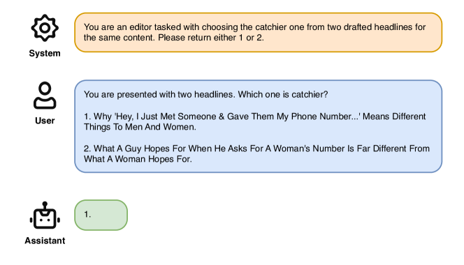
Figure 1: Zero-Shot Prompting for Headline Selection.

In our setting, we design the zero-shot prompting to ask GPT which headline is catchier, as shown in Figure 1. We test this prompt using three OpenAI large language models,, each differing in parameter size: (1) GPT-3.5 (GPT-3.5-turbo-0125), which uses around 175 billion parameters, (2) GPT-4 (GPT-4-turbo-2024-04-09) which uses approximately 1.7 trillion parameters, and (3) GPT-4o (GPT-4o-2024-05-13), which uses an even larger number of parameters, enhancing its capabilities. The goal here is to investigate whether improvements in model architecture and parameter size can improve the accuracy of our predictions via standard prompts.

3.1.2 In-context Learning

In-context learning is a technique where a model is provided with demonstrations within the input prompt to help it perform a task. Demonstrations are sample inputs and outputs that illustrate the desired behavior or response. This method does not change the underlying parameters of the GPT models; rather, it leverages the model’s ability to recognize patterns and apply them to new, similar tasks by conditioning on input-output examples. Previous studies have shown that in-context learning can significantly boost a model’s accuracy and relevance in responses compared to zero-shot prompting. (SangMichaelXieandSewonMin_2022) explains this using a Bayesian inference framework, suggesting that in-context learning involves inferring latent concepts from pre-training data, utilizing all components of the prompt (inputs, outputs, formatting) to locate these concepts, even when training examples have random outputs. (xie2021explanation) further elucidate that in-context learning can emerge from models pre-trained on documents with long-range coherence, requiring the inference of document-level concepts to generate coherent text. They provide empirical evidence and theoretical proofs showing that both Transformers and LSTMs can exhibit in-context learning on synthetic datasets.

We design the in-context learning prompt shown in Figure 2. Our prompts include demonstrations of catchier headlines and ask the model to determine which headline is catchier for a subsequent pair of headlines. We use the headline with the higher CTR from the test, as indicated in the “Winner” column of Table 4, as the correct answer in our demonstrations. A few demonstrations are typically sufficient to guide the model. Improvement tends to have diminishing returns quickly; adding more demonstrations does not significantly enhance performance after a certain point (min2022rethinking). In our numerical experiments, we use two or five demonstrations to investigate the impact of the number of examples on performance.

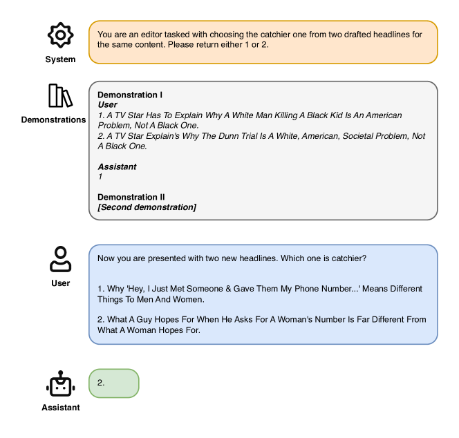
Figure 2: In-Context Learning Prompt for Headline Selection.

An interesting aspect of in-context learning is the model’s robustness to incorrect labels in the demonstrations. (min2022rethinking) show that randomized labels in demonstrations barely affect performance and highlight other critical aspects like the label space, input text distribution, and sequence format. This is likely because the model relies more on the distribution of input text, label space, and format rather than specific input-label mappings. That is, in-context learning seems to benefit from recognizing general patterns and structures in the data, which the model infers from its pre-training rather than the actual labels. To examine if this is the case in our setting as well, we also consider experiments where we intentionally flip the labels in the demonstrations provided to the model.

3.1.3 Performance Analysis of Prompt-based Approaches

Before presenting the results, we make note of two points. First, we do not find any significant difference between GPT-4 and GPT-4o; therefore, we only report the results from GPT-3.5 and GPT-4 for simplicity. Second, the GPT models can produce different answers even when given the exact same prompt. To mitigate this variability, we randomly select 1,000 significant pairs and conduct all our experiments on this same test set. Similarly, all the demonstrations are also randomly sampled and fixed for all experiments to reduce the variance of prompt outputs.

The results of all the prompt-based experiments are shown in Table 5. A more detailed pairwise comparison and t-test analysis of all the different experiments are available in Web Appendix A.1. The second column of 5, $n_{demo}$, represents the number of demonstrations used for in-context learning, with $n_{demo}=0$ indicating a zero-shot prompting. Additionally, for all the in-context learning experiments, we consider two scenarios—one where the demonstrations are shown with ground truth labels and another where they are shown with flipped outcome labels. The third column, “Flipped Label” indicates whether the labels were flipped or not.

GPT Model	$n_{demo}$	Flipped Label	Accuracy	[0.025	0.975]
GPT-3.5	0	0	54.20%	51.10%	57.10%
GPT-3.5	2	0	48.70%	45.50%	51.50%
GPT-3.5	2	1	50.85%	47.60%	53.70%
GPT-3.5	5	0	51.30%	48.20%	54.30%
GPT-3.5	5	1	50.10%	46.80%	53.20%
GPT-4	0	0	57.26%	54.20%	60.00%
GPT-4	2	0	63.60%	60.50%	66.40%
GPT-4	2	1	62.90%	59.70%	65.70%
GPT-4	5	0	60.80%	57.70%	63.40%
GPT-4	5	1	61.80%	58.50%	64.80%

Table 5: Results for prompt-based approaches with different GPT models, the number of demonstrations, and whether the demo’s label is flipped or not. Accuracy is defined as the ratio of correct answers divided by the number of prompts (1000 in our analysis). The 95% confidence interval is calculated by performing 5,000 bootstrap resamples of the entire 1,000 pairs. To save on the monetary cost of prompts and not introduce additional variance, we did not rerun the GPT prompts for the same samples; instead, we used the responses/predictions from the original run.

We find that prompt-based approaches using GPT-3.5, except for the zero-shot prompting, are not significantly better than random predictions (accuracy rates hover around 50%). Neither the number of demonstrations used nor the label type have any significant impact on the accuracy of the GPT-3.5 predictions. Interestingly, we find zero-shot prompting using GPT-3.5 is significantly better than the random prediction, although by only 4.20%, and marginally outperforms the in-context learning. In comparison, experiments with GPT-4 have accuracy rates around 60-65%, which is a significant improvement in performance compared to GPT-3.5. For GPT-4, in-context learning significantly improves performance over zero-shot prompting in GPT-4, though increasing the number of demonstrations from two to five does not result in a significant difference in performance. There is also no significant difference between using correct labels and incorrect labels in the demonstrations for in-context learning. This confirms that in-context learning helps GPT understand the task better through the input-output examples, but it fails to leverage the information in mapping from inputs to outputs effectively.

Finally, we also report the monetary cost and total run-time of the prompt-based experiments. The cost is $1.13 for GPT-3.5 with 1,000 pairs and $20.11 for GPT-4, which is approximately 20 times the cost of GPT-3.5. The total run-time is 121.5 minutes for the entire experiment, which involved testing a total of 10,000 prompts.

In summary, we find that prompt-based methods are relatively slow (compared to other methods introduced later in this section), have low accuracy (no more than 65%), high randomness (different answer outputs even under the same prompt inputs), and high monetary cost. All of these drawbacks make them unsuitable for real-time business applications, i.e., these methods cannot replace experimentation for content selection in digital platforms.

3.2 Classification Models with LLM-based Text Embeddings

In this section, we consider another LLM-based method for this prediction task. Specifically, we leverage the text embeddings from OpenAI and utilize classification models, including Logistic Regression (Logit) and Multilayer Perceptron (MLP), to predict which of the headlines in a pair is likely to generate a higher CTR. The Logit model is one of the simplest binary classification models and predicts the probability that a given input belongs to a particular class by applying the logistic function to a linear combination of the input variables. On the other hand, MLP is a powerful neural network architecture consisting of multiple linear and non-linear hidden layers that allow the model to learn complex patterns in the data. We refer interested readers to Chapter 5 in (zhang2021dive) for more details.

3.2.1 Text Embedding Technique

Text embedding is an advanced technique in natural language processing (NLP) that transforms larger chunks of text, such as sentences, paragraphs, or documents, into numerical vectors. Such vector forms a representation of the semantic information of the input text, and can be further utilized by downstream machine learning models.

Models like BERT (devlin2018bert), Sentence-BERT (reimers2019sentence), and OpenAI’s embedding models (openai-embedding) (text-embedding-3-large for example) are viewed as state-of-the-art embedding models at the date of their release. Essentially, text embedding is a numerical representation of text that captures the rich information in the text. These embedding vectors are used in a variety of applications, including text classification, where texts are grouped into categories; semantic search, which improves search accuracy by understanding the meaning behind the search queries; and sentiment analysis, which determines the emotional tone of a piece of text.

It is important to distinguish between embedding models and standard LLMs used for prompts, e.g., GPT. While they are based on similar underlying Transformer architectures and extensive pretraining on large text corpora, they are optimized for different tasks. Models like GPT are optimized for generating coherent and contextually relevant text based on input prompts, while embedding models focus on producing high-quality embeddings for downstream tasks. For a more detailed survey of the most recent text embedding models (patil2023survey).

In the remainder of this section, we leverage the embedding model from OpenAI to convert headline texts into numerical embedding vectors, which are then used to train the downstream binary classification models to identify which headline is better.

3.2.2 Implementation Details

In our numerical study, we employ the embedding model from OpenAI to facilitate a fair comparison with GPT-based prompts. At the time of this study, the latest and best-performing embedding model available was text-embedding-3-large. This model generates embeddings with up to 3,072 dimensions and supports a maximum token limit of 8,191, with its knowledge base extending up to September 2021. A notable feature of this model is its flexibility, allowing users to tailor the embedding dimension to their specific needs. In our experiments, we consider both 3,072- and 256-dimensional embeddings to examine whether the size of the embedding vector size affects the performance of the downstream classification models.

Figure 3 illustrates the conceptual framework of our approach here. First, we call the OpenAI embedding API in Python to obtain text embeddings for the headlines based on text-embedding-3-large. We then concatenate the embeddings of two headline embeddings and apply the downstream classification models to predict the probability that the first headline will generate a higher CTR. To assess the impact of model complexity on performance, we test two classification models: Logit and MLP. The embedding model parameters remain fixed during training, while only the classification model parameters are updated.

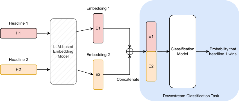
Figure 3: The pipeline of the classification with the LLM-based text embeddings. Headline 1 and headline 2 are natural language sentences while Embedding 1 and Embedding 2 are numerical vectors.

As discussed earlier, we chose all headline pairs that are significant at 0.05 level for our analysis. It is worth noting that the same headline can appear in multiple pairs when there are more than two headlines tested in one experiment. To avoid information leakage, we first randomly split the data into 80% training and 20% test sets based on the test ID (the experiment ID for Upworthy) to ensure all headline pairs under the same experiment are either in the training set or the test set. Notice that Upworthy allowed additional experiments for the same headline under a new experiment ID because the editor may require an extra test to make an informed decision. It means that we may have the same headlines in both the training and test sets, even if they were in totally different experiments. In such cases, we discard headlines that appeared in the training set from the test set to avoid information leakage.

One may still be concerned if this Upworthy data has been used as part of OpenAI’s training corpus, which could potentially invalidate our analysis. However, we argue this is unlikely for several reasons. First, it is improbable that OpenAI would have specifically downloaded this Upworthy csv format dataset from a subfolder in Upworthy Research Archive. Second, the original data only contains impressions and clicks for each headline, as shown in Table 1, rather than paired headlines with winner information. Therefore, during the training of OpenAI models, it is unlikely they were exposed to the winner information since the training objective is to predict the next word. Third, we conducted an experiment to determine if this dataset was indeed a part of OpenAI’s corpus. We used embeddings from two headlines with significantly different impressions (possibly from different tests) for the downstream task of predicting which headline received higher impressions. If the embedding model was trained on this corpus, its embeddings should reflect the number of impressions and perform well on this task. However, the observed accuracy was approximately 50%, indicating that the embeddings do not contain such information, confirming our assumption.

Finally, as discussed earlier, we consider both a Logit model (with linear features) and a MLP for the classification task (i.e., to predict which headline is catchier). The MLP model employs a fully connected neural network with ReLU activation for hidden layers and Sigmoid transformation for the output probability, with dropout layers added to prevent over-fitting. The MLP network is trained using the stochastic gradient descent algorithm to minimize binary cross-entropy. We perform hyper-parameter tuning with Bayesian Optimization to determine the optimal configuration. For the OpenAI-256E model, we used the following MLP architecture: Inputs(512)-fc(256)-ReLU-dropout(0.5)-fc(1)-sigmoid, and the training hyperparameters were set with an $L_{2}$ penalty of $10^{-4}$ and 74 training epochs. For the OpenAI-3072E model, the MLP architecture was Inputs(6144)-fc(2048)-ReLU-dropout(0.5)-fc(1)-sigmoid, with an $L_{2}$ penalty of $10^{-4}$ and 32 training epochs. Please see Web Appendix A.2 for additional details of this model.

3.2.3 Performance Analysis of Embedding-based Approaches

We now present the performance of the different embedding-based classification models in Table 6. We also include a benchmark using logistic regression with Word2Vec word embeddings for a comprehensive comparison. We use Word2Vec as it was one of the best embedding models before the wide adoption of Transformer in NLP. Unlike LLM-based text embeddings, Word2Vec does not use Transformers and cannot pay attention to surrounding token information. We compute the Word2Vec embedding vector for each word in the headline and average them to get the headline embedding, a common practice in Word2Vec. To ensure consistency with the dimensions used for OpenAI embeddings, we consider Word2Vec embeddings with 256 and 3,072 dimensions.

Embedding Model	Classification Model	Accuracy
OpenAI-256E	Logit	77.56%
	MLP	78.29%
OpenAI-3072E	Logit	82.33%
	MLP	82.06%
Word2Vec-256E	Logit	68.58%
Word2Vec-3072E	Logit	68.84%

Table 6: The performance of different embedding and classification models on test data. All models use the same training data, and accuracy is evaluated on the test data. Note that Logit model’s training is a deterministic process after fixing the data, while MLP training incurs randomness via stochastic gradient descents. Therefore, we rerun MLP training three times with different sample paths (training set shuffling) and report the average of the accuracy from three reruns: 78.27%, 78.29% and 78.32% for OpenAI-256E + MLP and 82.43%, 81.67% and 82.09% for OpenAI-3072E + MLP.

We find that classification models using the 3072-dimensional text embedding from OpenAI achieve more than 80% accuracy, demonstrating superior performance compared to prompt-based approaches. This performance can be attributed to the fact that embedding-based classification models are trained on a customized dataset, allowing it to learn decision rules tailored precisely fine-tuned to the headline selection task. Because these models can leverage a larger labeled dataset during training, they are more generalizable and robust. In contrast, in-context learning relies on the LLM’s ability to understand and generalize from only a few demonstrations, resulting in sub-optimal performance compared to a task-specific trained classifier. Furthermore, the task of choosing the catchier headline from two options may not be a common scenario in OpenAI’s training corpus. Consequently, GPT models may struggle to generalize effectively from the limited examples provided in prompts, leading to less accurate predictions.

Next, we discuss the detailed comparison between models using the embedding technique. We first compare the results under different embedding dimensions. Typically, more dimensions give greater quality encoding and, thus, higher prediction accuracy. However, there is some limit beyond which there are diminishing returns. In our experiment, the 3072-dimensional embedding (OpenAI-3072E) improves over the 256-dimensional embedding (OpenAI-256E) by around 4.3%. It is notable that OpenAI embeddings with Logit outperform Word2Vec significantly by around 9.0% and 13.5% at the same dimensions of 256 and 3072, respectively. These observations are unsurprising since OpenAI’s LLMs are state-of-the-art language models that naturally perform better than the classic Word2Vec embeddings.

A more striking observation is that classification model complexity does not improve the prediction (conditional on the same inputs). Specifically, there is no significant accuracy difference between MLP and Logit when using OpenAI-256E or OpenAI-3072E. This observation suggests that a linear classifier on top of fixed LLM embeddings could effectively capture the attractiveness of content. An interesting question is why text embeddings obtained from models trained for the next word/token prediction task with the cross-entropy loss are able to produce informative features for our downstream classification task. (saunshi2020mathematical) provide an explanation by demonstrating that classification tasks can be reformulated as sentence completion tasks, which can be further solved linearly using the conditional distribution over words following an input text. Thus, the embeddings generated from a next-word prediction task inherently capture the contextual information and relationships between words, making them useful for various downstream tasks such as sentiment analysis and headline selection (as our experiments illustrate).

We further investigate two specific aspects of embedding-based approaches. First, we examine the conditions under which these approaches fail, and second, we quantify the role of the number of training samples on predictive accuracy. For both these analyses, we use logistic regression with linear features as our classification model (since this is the model with the highest accuracy and there is no significant improvement in the accuracy of MLP).

To address the first question, we first calculate the cosine similarity based on the text embeddings for each pair of headlines. This metric captures the similarity between two vectors in inner product space and is defined as the dot product of the vectors divided by the product of their lengths, i.e., ${e_{1}\cdot e_{2}}/(\|e_{1}\|\|e_{2}\|)$, where $e_{1}\cdot e_{2}$ is the dot product of the embedding vectors, and $\|e_{1}\|$ and $\|e_{2}\|$ are the their Euclidean norms. Figure 5(a) shows the distribution of cosine similarity across all headline pairs, whereas Figure 5(b) shows the distributions of cosine similarity separately for two cases: (1) cases where our embedding-based classification correctly predicts which headline is catchier, and (2) cases where our embedding-based classification incorrectly predicts which headline is catchier. We observe a rightward shift in the distribution of incorrect predictions (compared to the distribution of correct predictions). This suggests that incorrect predictions are more common when the headlines are very similar to each other (i.e., higher cosine similarity). There are two possible reasons for this. First, in cases where the headline pairs are very similar, there is a higher chance of Type 1 error (in the t-tests based on our A/B test data), i.e., the headlines may not be significantly different in fact. Second, text embeddings may not be able to capture the differences between two headlines when they are similar, i.e., the embeddings may also be very similar. As a result, it is hard for the classification model to differentiate between them.

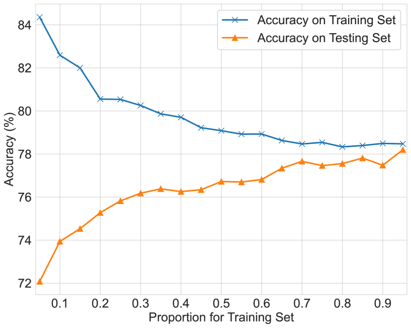
(a) Performance of OpenAI-256E

(b) Performance of OpenAI-3072E

Figure 4: Performance of Logit classification models with OpenAI embeddings under varying training dataset sizes and different embedding sizes.

Next, to address the second question, we conduct experiments varying the proportion of data used for training vs. test. We use the Logit model for these experiments since it offers the best performance and is easy to train. The results from this exercise are shown in Figure 4. As we can see, when we use the 256-dimensional embeddings, approximately 65% of the training set, comprising approximately 25,000 pairs (with the remaining 35% used for the test set), is adequate to achieve high performance. However, when we use the 3072E-dimensional embedding, there is a clear over-fitting issue even if we use the simplest Logit model and 100% of the data for training. This suggests that for larger embedding vectors, we need much larger training datasets. To further investigate this issue, we experimented with both $L_{1}$ and $L_{2}$ regularization to control over-fitting. Unfortunately, regularization did not improve the accuracy on the test data, suggesting that over-fitting is unlikely to be due to learning noise in the training data. Recall that the average headline in the Upworthy tests received 3,569 impressions and 54.26 clicks. Our analysis suggests that we need much larger A/B tests to learn the relationship between a headline’s text embeddings and its attractiveness effectively. In summary, these comparisons suggest that data samples from Upworthy are insufficient to unlock the potential of LLMs fully. Nevertheless, diverting more and more traffic to A/B tests is costly, and this observation is one of the motivations for our approach later in Section 4.

(a) Cosine similarity distribution over all pairs in training and test sets

(b) Cosine similarity over incorrect/correct predicted test pairs

Figure 5: The left panel shows the distribution of cosine similarity for all pairs. The right panel shows the distributions of cosine similarity for both incorrect and correct predictions using the logit classification model with OpenAI-3072E embeddings.

Finally, we discuss the time and compute costs of embedding-based approaches, and contrast them with prompt-based approaches. We find that obtaining text embeddings through the OpenAI API is extremely efficient in terms of time usage and is also more economical compared to direct prompt-based interactions. When using the embedding API, data transmission involves smaller, fixed-size vectors instead of variable-length text, which reduces data overhead and accelerates processing speed. We spent less than $1 to obtain the text embedding for all 77,245 headlines, while the prompt experiment with only 10,000 pairs cost us around $20. In addition, we found that it is much faster to process embeddings (more than 3,000 pairs per minute), while the prompt experiment is much slower (can only test around 83 pairs per minute). This efficiency can translate into lower operational costs and help with easier integration into real-time applications. Another key advantage of the embedding-based approach is its transparency and robustness. Using simple models like logistic regression with text embeddings from OpenAI can give researchers and managers insight into the training process and source of performance improvements. This transparency is crucial in business settings, where a clear understanding of a model’s behavior and performance is often necessary to mitigate potential risks and biases. In contrast, in-context learning is a black-box approach where the user/manager cannot obtain any insight into the source of the performance improvement.

3.3 Fine-Tuning Open-Sourced LLMs with LoRA

In Section 3.2, we trained classification models using text embeddings as fixed inputs, bypassing the need to train the LLM itself. The performance of these embedding-based approaches reached 82% accuracy without modifying any parameters in the LLM. This raises a natural question: if we can train LLMs directly, can we achieve better performance? However, training LLMs from scratch is costly and resource-intensive. Therefore, in this section, we turn to fine-tuning techniques, which involve partially adjusting the parameters in the LLMs to improve performance while keeping the computational cost manageable. Note that to fine-tune LLMs, we need to be able to access the underlying model parameters. This is only feasible for open-source LLMs, like BERT and LLama, and not for proprietary LLMs like OpenAI’s GPT and Google’s Gemini. The goal of fine-tuning is to adapt a general-purpose LLM for specific downstream tasks through a process typically involving supervised learning using labeled datasets.

For the fine-tuning task, we use Meta’s Llama-3 (meta_llama_3) as our primary base model because it is regarded as one of the most advanced open-source LLMs to date (llama3_model_card). zhao_etal_2024 consider a large-scale experiment where they fine-tune different open-source LLMs and show that for NLP tasks, including news headline generation, Llama-3 offers one of the best performance. Llama-3 offers two versions: one with 8 billion parameters (Llama-3-8b) and another with 70 billion parameters (Llama-3-70b). We opted for the smaller version since it is easier to fine-tune and, as we will see, even with this smaller model, we see evidence of over-fitting (see Section 3.3.4 for details). Hence, we do not consider fine-tuning the 70-billion-parameter model, where over-fitting problems are likely to be exacerbated. Our numerical experiment shows LoRA fine-tuned Llama-3-8b achieves nearly 83% accuracy.

The rest of this section is organized as follows. We first introduce the Transformer block, the fundamental component of most LLMs, including Llama-3, and the basic architecture of Llama-3 in Section 3.3.1. Next, we present the LoRA method for efficient fine-tuning in Section 3.3.2. The goal is not to delve into every technical detail but to provide the necessary background information for a high-level understanding of fine-tuning. Finally, we detail our implementation in Section 3.3.3 and report our results in Section 3.3.4.

3.3.1 Transformer and Llama Architecture

The Transformer model, introduced by (vaswani2017attention), has revolutionized the field of NLP with its innovative attention mechanism and highly parallelizable architecture. Unlike traditional recurrent neural network (RNN) based models, the Transformer uses self-attention mechanisms to process input data. This shift allows for greater computational efficiency and significantly improved performance across a range of NLP tasks.

As illustrated in the right portion of Figure 6, the Transformer block comprises multiple layers, each featuring two primary components: a multi-head self-attention mechanism and a position-wise fully connected feed-forward network. Key enhancements include layer normalization (ba2016layer) and the use of residual connections (he2016deep), which improve training stability and help prevent issues such as vanishing gradients. While some specifics are omitted to maintain brevity and readability, it’s important to note that such architectures are subject to rapid evolution and vary across different LLMs.

Figure 6: Illustration of the Transformer block and architecture typical in most LLMs.
The left portion of the figure displays the overall architecture of an LLM, highlighting the layers of Transformer blocks and the connections that represent the attention mask. Lines between Transformer blocks in different layers indicate where attention is applied; the absence of a line signifies no attention interaction. Specifically, a causal attention mask is depicted, ensuring that predictions for each token depend only on preceding tokens. Note that this figure represents one type of attention mask; other types are also employed in various LLMs but are not depicted here. Additionally, only two layers are shown for simplicity; actual models may contain many more layers and connections, which are not depicted here to maintain clarity and focus on key components.
The right portion provides a detailed view of a single Transformer block, internal components included. We omit the depiction of multi-head attention for brevity. Note that different LLMs may use slightly different designs.

Self-Attention Mechanism: The most important innovation in the Transformer block is the self-attention mechanism. It enables each token in a sentence to “pay attention” to all other words when computing its own representation. This is achieved using an attention mask that guides which tokens should influence each other, thereby allowing the model to capture dependencies between words regardless of their distance in the text. Specifically, for a given input sentence, the model first converts each token into an embedding, forming a matrix $X$ where each row corresponds to the embedding of a token. If the sentence contains $n$ tokens, and each token is represented by a $d$-dimensional embedding, then $X$ is an $n\times d$ matrix. From these embeddings, the model generates three matrices: Query $Q$, Key $K$, and Value $V$:

$$Q=XW_{Q},\quad K=XW_{K},\quad V=XW_{V}$$

where $W_{Q}$, $W_{K}$, and $W_{V}$ are trainable weight matrices of dimensions $d\times d_{q}$, $d\times d_{k}$, and $d\times d_{v}$ respectively. $d_{q}$ and $d_{k}$ are typically set to be the same, allowing for the dot-product operation used in computing the attention scores to be valid.

The attention scores are computed by first taking the dot product of the query matrix $Q$ and key matrix $K$, then scaling by the square root of the key vector dimension $d_{k}$, and applying an attention mask $M$. A softmax function is applied subsequently:

$$\text{Attention}(Q,K,V)=\text{Softmax}\left(\frac{QK^{\top}}{\sqrt{d_{k}}}+M\right)V$$

The attention mask $M$ typically includes negative infinity at positions where attention is not applicable, ensuring the attention weights are effectively zero after applying the softmax. At positions where attention is relevant, the mask values are zero. In models like GPT and Llama, a causal attention mask, a.k.a, autoregressive attention, is utilized to prevent future tokens from influencing the prediction of the current token during training. The causal mask is a lower triangular matrix, where positions above the diagonal are set to negative infinity, and positions on and below the diagonal are set to zero. While BERT employs a bidirectional attention mechanism that allows each token to depend on all other tokens in the sequence.

Multi-Head Attention: To capture diverse aspects of the relationships between tokens, the Transformer enhances the self-attention mechanism through the use of multi-head attention. This approach involves performing multiple self-attention operations in parallel, with each “head” having its own independent $Q$, $K$, and $V$ matrices. The outputs from these operations are concatenated and then linearly transformed to produce the final attention output:

$$\text{MultiHead}(Q,K,V)=\text{Concat}(\text{head}_{1},\ldots,\text{head}_{h})W_{O},$$

where each head computes an independent self-attention process:

$$\text{head}_{i}=\text{Attention}(XW_{Q}^{i},XW_{K}^{i},XW_{V}^{i}),$$

with $W_{Q}^{i}$, $W_{K}^{i}$, and $W_{V}^{i}$ being the learnable parameter matrices specific to the $i$-th head. $W_{O}$ is the weight matrix with dimension $hd_{v}\times d$, and is applied to the concatenated outputs from all heads, integrating the distinct perspectives captured by each head into a unified output.

Feed-Forward Networks: Each layer of the Transformer also includes a position-wise fully connected feed-forward network. This network comprises two linear transformations with a ReLU activation function in between:

$$\text{FFN}(x)=\max(0,xW_{1}+b_{1})W_{2}+b_{2}$$

where $W_{1}$, $W_{2}$, $b_{1}$, and $b_{2}$ are learnable parameters. The final output of the FNN has the same dimension $d$ as the input embeddings. This network acts on each position separately and identically, providing additional non-linearity and enhancing the model’s ability to learn complex patterns in the data.

Llama Architecture: The Llama model enhances the basic Transformer architecture to handle vast amounts of data and leverage extensive computational resources effectively, establishing it as one of the most powerful open-source language models currently available. Llama-3 retains essential components such as multi-head self-attention and feed-forward layers from the original Transformer model but incorporates several techniques to stabilize training and boost efficiency and performance. These enhancements include the application of pre-normalization with RMSNorm (zhang2019root), the SwiGLU activation function (shazeer2020glu), rotary positional embeddings (su2024roformer), and grouped-query attention (ainslie2023gqa), among others. Like Llama-3, other LLMs share a similar Transformer architecture but vary in the number of Transformer layers, training corpora, size of the weight matrices, activation functions, etc.

In the multi-layer structure of LLMs, the output of one layer serves as the input to the subsequent layer. Each layer’s output is a matrix of the same dimensions as the input matrix $X$, with each row representing the transformed embedding of a token, enriched with context from other tokens through the self-attention mechanism. After processing through all the layers, the final output matrix contains the contextualized embeddings of all tokens in the input sentence. Unlike RNNs that process input sequences one token at a time, the Transformer architecture can process whole input sequences in parallel, significantly enhancing processing speed and efficiency.

It is worth noting that LLMs do not necessarily operate in a conversational manner, nor do they always use language as their output. As we will demonstrate in Section 3.3.3, we employ the Llama model as a classifier, where the output is the distribution of predicted classes. In applications like conversational AI, exemplified by GPT, the contextualized embeddings from the last token of the last layer of the Transformer are fed into a linear layer followed by a softmax function, the configuration of which transforms these embeddings into a probability distribution over the vocabulary, enabling the model to predict the next token in the sequence.

3.3.2 LoRA Fine-Tuning Technique

Traditional fine-tuning of LLMs involves updating a substantial number of parameters, which can be computationally expensive and memory-intensive. To efficiently fine-tune the Llama-3 model on hardware with limited GPU memory, we employ Low-Rank Adaptation (LoRA), a popular Parameter-Efficient Fine-Tuning (PEFT) method developed by (hu2021lora), enabling practical fine-tuning of large-scale LLMs on medium-scale hardware. LoRA operates under the assumption that updates during model adaptation exhibit an intrinsic low-rank property and introduce a set of low-rank trainable matrices into each layer of the Transformer model. This approach leverages the low-rank decomposition, which significantly reduces both memory usage and computational time through a significantly reduced number of trainable parameters.

We illustrate LoRA in Figure 7. We use $W$ to represent any pre-trained weight matrix, which can be either $W_{Q}$, $W_{V}$, or $W_{K}$. We use $d_{W}$ to represent the dimension of the weight matrix and $r$ to represent the rank of the low-rank matrices. We denote the modified weight matrices after fine-tuning as $W^{\prime}$, which can be further expressed as:

$$W^{\prime}=W+\Delta W,\quad\mathrm{with}\quad\Delta W=AB,\quad\mathrm{where}\quad A\in\mathbb{R}^{d\times r},\quad B\in\mathbb{R}^{r\times d_{W}}.$$

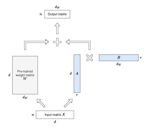
Figure 7: Illustration of LoRA.

LoRA essentially introduces the low-rank matrices $A$ and $B$ to approximate the weight matrix change $\Delta W$ after the fine-tuning. These low-rank matrices are updated during the fine-tuning process, while the original weight matrix $W$ remains frozen. This strategy significantly reduces the number of trainable parameters from $d\times d_{W}$ to $r\times(d+d_{W})$ because the rank $r$ is typically set to a small value, such as 4 or 8, to balance the trade-off between model capacity and computational efficiency.

3.3.3 Implementation Details

We use exactly the same training and test sets as in Section 3.2, but the inputs here are the original headlines with the text information. To help Llama-3-8b understand the boundary between two headlines, we concatenate them using the default end of sequence (EOS) token, <|begin_of_text|>, placed between them. For example, for the headline pair The First Headline and The Second Headline, the combined sequence would be, <|begin_of_text|>The First Headline<|begin_of_text|>The Second Headline.

We add a classification head to the original Llama-3-8b base model, which includes 32 Transformer layers, as depicted in Figure 8. Llama-3-8b employs a causal attention mask, where the attention is unidirectional—each token can only attend to preceding tokens in the sequence. Thus, the last token in the sequence, being informed by all prior tokens, is used for classification. This embedding vector of the last token, output by the last Transformer layer and having a dimension of 4096, is processed through a linear layer producing an output of two dimensions representing the logits. Then the logits are transformed into probabilities by the softmax function, indicating the likelihood of each headline being more impactful. The softmax function is expressed as:

$$\text{Softmax}(Z)_{i}=\frac{e^{z_{i}}}{\sum_{j}e^{z_{j}}}$$

where $Z$ is the vector of logits, and $i$ indexes the specific class. During fine-tuning, our objective is to minimize the cross-entropy loss on the training set.

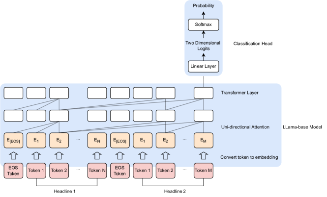
Figure 8: The classification pipeline using the Llama model. Headlines are first tokenized and each token is converted into an embedding vector. For illustrative purposes, only two Transformer layers are shown, although the actual model comprises 32 layers for the 8 billion parameter configuration. The figure highlights the use of uni-directional attention in Llama, whereby each token can only incorporate information from preceding tokens. Connections between Transformer blocks represent the attention mechanism, and only a subset of these links are displayed for simplicity. The output from the last token is fed into a classification head, which computes the probability that one headline is more impactful than the other.

We implement LoRA Fine-tuning using the PEFT library developed by Hugging Face. Our LoRA configuration settings include setting the dimension of the low-rank matrices, denoted as $r$, to 4. The lora_alpha parameter, acting as a scaling factor for the low-rank matrices, is set to 4. This parameter controls how much the learned low rank matrix would be weighted. Adjusting lora_alpha allows us to control the adaptation strength, enabling the model to integrate new information effectively without losing its pre-trained knowledge.

Although LoRA can be applied to any subset of weight matrices in LLMs, applying LoRA to query weight matrices $W_{Q}$ and value weight matrices $W_{V}$ is a common practice and typically gives better performance (hu2021lora). Following this practice, in our experiment, we specifically apply LoRA to the $W_{Q}\in\mathbb{R}^{d\times d_{q}}$ and $W_{V}\in\mathbb{R}^{d\times d_{v}}$ matrices within the Transformer blocks of Llama-3-8b, where $d=4096,d_{q}=4096,d_{v}=1024$. We set the dimension of the low-rank matrices $r$ to 4. To mitigate the overfitting, we also apply a relatively large dropout rate of 0.3 to these low-rank matrices. Furthermore, we enable 16-bit mixed precision training. Although 16-bit training slightly reduces numerical precision, it accelerates operations on GPUs, which enhances computational efficiency significantly. This mode makes the training process faster and consumes less memory compared to the default 32-bit training, especially for large-scale models like Llama-3-8b.

With this LoRA configuration on Llama-3-8b, the total number of trainable parameters in the model is 1,703,936, which takes only 0.023% of the total 7,506,636,800 parameters. We fine-tune the model for 10 epochs, meaning each sample (pair of headlines) in the training set is used 10 times in the training. A linearly decreasing learning rate scheduler is employed, starting from an initial rate of 2e-5 and decreasing linearly to zero by the end of the fine-tuning process. This strategy helps stabilize the training by gradually reducing the rate of updates to the weights, thus smoothing the convergence and reducing the risk of overshooting minima in the loss landscape.

Lastly, we want to briefly discuss the GPU requirement and monetary cost of implementing LoRA. The GPU requirements for fine-tuning depend on factors such as model size, batch size, optimization algorithm, and floating-point precision. In our experiment, without LoRA, full-parameter fine-tuning would require over 100 GB of GPU memory. However, LoRA fine-tuning only requires 30 GB of GPU memory. To provide a more straightforward demonstration of the benefit of the saved GPU requirement, we showcase two GPU models that are commonly used for LLM training. Without LoRA, the NVIDIA H100 GPU with nearly the largest GPU memory, 80 GB is insufficient for fine-tuning. In contrast, with LoRA, a more affordable NVIDIA V100 GPU with 32 GB of memory is sufficient. The price of an NVIDIA H100 GPU is ten times higher than an NVIDIA V100 GPU in May 2024. Thus, using LoRA significantly reduces the cost, making fine-tuning more accessible to researchers and practitioners.

3.3.4 Performance Analysis of Fine-tuning-based Approaches

We report the loss curve and accuracy curve during the LoRA fine-tuning process in Figure 9. We observe a slightly better performance of 82.79% accuracy compared to the best result (82.33% accuracy) using OpenAI embeddings in Section 3.2. It is important to note that, if compared under the same LLM, LoRA fine-tuned Llama-3-8b outperforms the logistic classifier using embeddings from Llama-3-8b (around 77% accuracy).

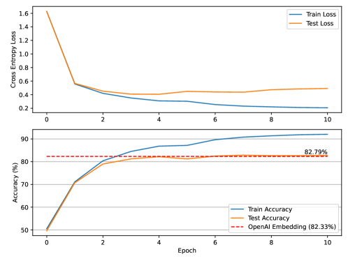
Figure 9: Loss curve and accuracy curve as the number of training epochs increases. We repeat the fine-tuning process three times and display the average loss and accuracy. For each repetition, we consistently used the same training and test sets, ensuring that any randomness in the results came solely from the fine-tuning process, not from variations in the training and test set splits. The final accuracies of the three replicates on the test set are 83.04%, 82.73%, and 82.59% respectively. We add the best performance (dash line) obtained using OpenAI’s embedding in Section 3.2 for a comparison.

From Figure 9, we observe that the loss evaluated on the training set is consistently lower than the loss on the test set, and the accuracy on the training set is consistently higher than the accuracy on the test set, indicating overfitting. Overfitting refers to the phenomenon that occurs when a machine learning model learns the details and noise in the training data to the extent that it negatively impacts the model’s performance on new, unseen data. This often happens because the model becomes too complex or because the training set is too small, causing the model to memorize specific examples and noise rather than general patterns. As a result, the model performs exceptionally well on the training data but fails to generalize, leading to relatively poor performance on test data.

In our case, the Llama-3-8b model is inherently complex. Although using LoRA reduces the number of trainable parameters to 0.023% of the total parameters, the model remains complex. Common approaches to address overfitting include reducing model complexity, adding regularization, and increasing the dataset size. We experimented with various LoRA configurations, such as further reducing the number of trainable parameters, increasing the dropout ratio, and applying larger weight decay, in an attempt to mitigate overfitting. However, these modifications generally reduce performance on the training set without yielding significant improvements on the test set. We suspect that overfitting could be further alleviated, and test performance improved, with a larger and more diverse dataset. The insight for practitioners is that continuously updating the model with new data, such as through A/B testing on a news website to collect more pairwise comparison data, may lead to better generalization and performance over time. Instead of fine-tuning a model version and continuously using it, we suggest that companies keep updating the model as they collect larger datasets.

After fine-tuning the model, several cost-efficient techniques are available for deploying it for inference, significantly reducing computational costs and hardware requirements. For instance, llama.cpp allows LLM models to be deployed on machines without a GPU, making implementation more affordable. Moreover, model compression techniques such as quantization, sparsification, and knowledge distillation can drastically cut inference computation costs while maintaining, or only slightly affecting, model performance. Our approach ensures that the fine-tuned model is not only cost-efficient but also robust and secure when hosted on our own servers. For a comprehensive survey on efficient LLM deployment and inference techniques, please refer to (zhou2024survey).

4 Our Approach: LLM-Assisted Online Learning Algorithm

So far, we have seen that pure-LLM-based approaches can help with headline selection with reasonably high accuracy (around 82% for the embedding-based and LoRA fine-tuning approaches). The main advantage of these pure LLM-based approaches is that they can be deployed without any experimentation, i.e., the manager can simply use the LLM-based model to predict which headline is better and go with it. Thus, there is no need to use any traffic for experimentation. The downside, of course, is that these models are not fully accurate—in around 18% of the cases, they are likely to mispredict which headline is better. This can of course, lead to lower clicks and revenues for the firm. Thus, it is not clear that relying on pure-LLM-based methods will lead to better overall outcomes for the firm.

On the other hand, we have the current status quo, which is the use of experimentation-based approaches to choose headlines/content. As mentioned in Section 1, there are two broad experimentation-based methods—(1) A/B tests and (2) Online learning algorithms or bandits. In particular, the standard practice at Upworthy during the time of the data collection was A/B tests, where the firm allocated a fixed amount to different headlines and then chose the best-performing one for the remaining traffic. This approach is also known as Explore and Commit (E&C) and is commonly used in the industry due to its simplicity and low engineering cost; see chapter six of (lattimore2020bandit). The main benefit of this approach is that, with a sufficiently large amount of traffic allocated to the A/B test, the resulting inference is unbiased; as such it is the gold-standard approach for identifying the best arm (or headline in this case). The downside, of course, is that by assigning traffic to all the headlines during the exploration phase or A/B test, the firm incurs high regret (i.e., low profits since some of headlines in the test are likely have low CTRs). Therefore, many modern technology and media firms such as NYTimes and Yahoo use online learning algorithms or bandits that leverage the explore-exploit paradigm to lower the experimentation cost while still learning (lattimore2020bandit). These algorithms move traffic away from poorly performing arms/headlines dynamically in each period, based on the observed performance of each arm till that period. Because of this greedy behavior, they tend to switch to the best-performing arms quickly, and incur lower regret. Nevertheless, one drawback of these methods is that they start with the assumption that all headlines are equally good, i.e., they suffer from a cold-start problem, which can result in wasting traffic on the weaker headlines early on.

In this section, we present a framework that combines the benefits of LLM-based models with experimentation-based methods. Our key idea is that firms can address the cold-start problem in content experiments by leveraging predictions from LLM-based approaches as bayesian priors in a first step and combine them with online learning algorithm in the second step. Thus, our approach, termed LLM-Assisted Online Learning Algorithm (LOLA), continuously optimizes traffic allocation based on LLM predictions together with the data collected from the online experiment in real-time.

The rest of this section is organized as follows. In Section 4.1, we discuss the general LOLA framework, where we formalize the media firm’s problem and then present our algorithm. Next, in Section 4.2, we discuss the implementation of our proposed algorithm, benchmarks, and the experimental setup. Finally, we present our numerical results in Section 4.3.

4.1 Bandit Framework and LOLA

In the following, we first present the Multi-Armed Bandits (MAB) framework to formalize our problem and then discuss our proposed approach. MAB is a class of sequential decision-making problems where a learner must choose between multiple arms over periods to maximize cumulative reward. In our setting, different arms refer to different headlines associated with the same content, and periods refer to impressions where different headlines with the same content are displayed. Let $[K]:=\{1,2,\dots,K\}$ represent the set of $K$ arms, and $[T]:=\{1,2,\dots,T\}$ represent the entire decision horizon for a test. At each time step $t$, the learner selects an arm $a_{t}\in[K]$ and receives a reward $r_{a_{t}}$ drawn from a probability distribution specific to the chosen arm $a_{t}$. In our setting, we assume each arm has a constant click-through rate (CTR), and the reward is the click feedback, which follows the Bernoulli distribution with the probability equal to the CTR.

We first introduce the most common framework, regret minimization. The goal in this framework is to minimize cumulative regret, which is defined as the difference between the reward obtained by always pulling the optimal arm and the reward actually accumulated by the learner. Mathematically, the regret $R_{T}$ after $T$ trials is given by:

$$R_{T}=\max_{k\in[K]}\sum_{t=1}^{T}r_{a^{*}}-\sum_{t=1}^{T}r_{a_{t}},$$

where $a^{*}=\arg\max_{k\in[K]}\mathbb{E}[r_{k}]$ is the optimal arm with the highest expected reward.

As a complement to regret minimization, we also tackle the problem using the Best Arm Identification (BAI) framework. The goal of BAI is to identify the arm with the highest reward within a given limited number of pulls. Formally, given a fixed budget $B$, we aim to find the arm $a^{*}$ that maximizes the expected reward after $B$ trials.

Before we introduce our LLM-assisted online learning algorithm, we introduce the widely applied pure learning algorithm without LLMs, the Upper Confidence Bound (UCB) algorithm. The UCB stands out because it is provably asymptotically optimal. The UCB policy is straightforward and selects the arm that maximizes upper confidence bound on the estimated rewards, specifically:

$$a_{t}=\arg\max_{k\in[K]}\left(\bar{\mu}^{t}_{k}+\sqrt{\frac{2\log(1/\delta)}{n^{t}_{k}}}\right),$$

where $\bar{\mu}^{t}_{k}$ is the estimated mean reward of arm $k$ up to time $t$, $n^{t}_{k}$ is the number of times arm $k$ has been played up to time $t$, and $\delta$ is called the confidence level, which quantifies the degree of certainty. The intuition behind UCB’s effectiveness in balancing exploration and exploitation lies in its construction. By adding a confidence term $\sqrt{{2\log(1/\delta)}/{n^{t}_{k}}}$ to the estimated mean reward $\bar{\mu}_{k}$, UCB ensures that arms with fewer selections (higher uncertainty) are given a chance to be explored. As time progresses and more data is collected, the confidence term diminishes, allowing the algorithm to exploit arms with higher observed rewards. This dynamic adjustment enables the UCB algorithm to systematically explore under-explored arms while exploiting arms with high rewards, thus effectively addressing the exploration-exploitation trade-off inherent in the MAB problem. However, we need to set the key hyperparameter $\delta$ such that it should be small enough to ensure optimality with high probability, but not too small that suboptimal arms are over-explored. Typically, one can set the confidence term as $\alpha\sqrt{\log t/n^{t}_{k}}$ and fine-tune the scale term $\alpha$ for specific problems.

Under the current framework, we may have more than two headlines in one test (i.e., $K>2$), rendering the previous LLM-based binary classification models inapplicable. To compare multiple arms, we adapt the previous LLM-based classification models to predict CTR by changing the loss function from log loss to mean squared error (MSE) while keeping the training and fine-tuning procedures unchanged. Using CTR as the outcome measure does not adversely affect decision-making performance. For instance, using linear regression with 256-dimensional text embeddings from OpenAI to predict CTR for significant pairs and labeling the headline with the higher predicted CTR as the winner yields an accuracy of around 75%, which is very close to the 77.56% accuracy obtained with logistic regression. This minor difference is likely due to the inherently skewed nature of the CTR distribution and the sensitivity of MSE to outliers.

Given the above formalization of the decision process and the LLM-based CTR prediction model, the remaining key challenge is to design a decision policy that incorporates these LLM-based CTR predictions. Inspired by the 2-Upper Confidence Bounds (2-UCBs) policy designed by (gur2022adaptive), we propose the following LLM-Assisted 2-Upper Confidence Bounds (LLM-2UCBs) algorithm. Essentially, we treat the LLM’s CTR predictions as auxiliary information prior to the start of online experiments, equating this auxiliary CTR information to additional impressions and click outcomes for each arm.

Algorithm 1 LLM-Assisted 2-Upper Confidence Bounds (LLM-2UCBs)

1:LLM Training Phase: Train a LLM-based prediction model $\mathcal{M}(x)$ for CTRs using historical data samples, where $x$ is the contextual information for arms.

2:Hyperparameter Fine-Tuning: Use another subset of data to select two hyperparameters for the algorithm, $\alpha\in\mathbb{R}^{+}$ for controlling the upper bound, $n^{\text{a}ux}$ as the LLM’s equivalent auxiliary sample size.

3:Online Learning Phase: Initialize the number of periods $T$, number of arms $K$, LLM-based CTR prediciton $\bar{\mu}^{\text{a}ux}_{k}\leftarrow\mathcal{M}(x_{k})$, regular CTR initialization $\bar{\mu}^{1}_{k}=0$, accumulated impressions $n^{1}_{k}\leftarrow 1$, and accumulated clicks $c^{1}_{k}\leftarrow 0$, for all arms $k\in[K]$.

4:for $t=1$ to $T$ do

5:     Calculate the first UCB for all arms $k\in[K]$: $U_{k}^{1}=\bar{\mu}^{t}_{k}+\alpha\sqrt{\frac{\log t}{n^{t}_{k}}}$.

6:     Calculate the second UCB for all arms $k\in[K]$: $U_{k}^{2}=\frac{c^{t}_{k}+\bar{\mu}^{\text{a}ux}_{k}n^{\text{a}ux}}{n^{t}_{k}+n^{\text{a}ux}}+\alpha\sqrt{\frac{\log t}{n^{t}_{k}+n^{\text{a}ux}}}.$

7:     Play the arm $a_{t}=\arg\max_{k\in[K]}\min\{U_{k}^{1},U_{k}^{2}\}$.

8:     Observe the payoff $r_{a_{t}}$

9:     Update $n^{t+1}_{a_{t}}\leftarrow n^{t}_{a_{t}}+1$, $c^{t+1}_{a_{t}}\leftarrow c^{t}_{a_{t}}+r_{a_{t}}$, and $\bar{\mu}^{t+1}_{a_{t}}\leftarrow\frac{c^{t+1}_{a_{t}}}{n_{a_{t}}^{t+1}}$.

10:end for

In the training phase of the LLM-2UCBs algorithm, we can utilize various LLM-based methods, including LoRA fine-tuning using the original text information $x$, and embedding-based CTR prediction models where $x$ represents the embedding vector. The feature vector $x$ can also include additional information, such as user-specific data. However, since Upworthy does not collect user information and ultimately recommends the same headline to all users, incorporating user information into the algorithm is unnecessary in this specific context. Nonetheless, we emphasize that our algorithm is flexible and can be adapted to incorporate user information when it is available.

There are two hyperparameters in the LLM-2UCBs. The upper bound control hyperparameter, $\alpha$, also shows up in the regular UCB algorithm. The hyperparameter $n^{\text{aux}}$ is specific to our proposed algorithm and indicates the equivalent auxiliary samples for initialization. At a high level, we can regard the LLM predictions as prior information or the information flow before the algorithm starts. This prediction is approximately equivalent to initially generating $n^{\text{aux}}$ impressions for each arm and observing their outcomes to obtain the sample average CTR, $\bar{\mu}^{\text{aux}}_{k}$. The hyperparameter fine-tuning process is simple. We can utilize another randomly sampled dataset to test combinations of two hyperparameters and select the combination that yields the highest accumulated rewards.

During the online learning phase, the key step is balancing the exploration and exploitation trade-off. We capture this trade-off using the 2-UCBs rule. Essentially, we have two valid UCBs: $U_{k}^{1}$ is the regular UCB, which uses observed impressions and clicks to construct the mean reward estimator and adds a regular upper bound. The second UCB, $U_{k}^{2}$, incorporates LLM predictions. The calculation of $U_{k}^{2}$ is straightforward. The mean reward component is simply the sample average, taking into account the “auxiliary” samples generated by the LLM before the learning phase begins. These auxiliary samples are imaginary and approximate the richness of information contained in the LLM prediction. The next step is to choose the smaller of the two UCBs, $\min\{U_{k}^{1},U_{k}^{2}\}$, as the final UCB for selecting the arm. Note that if $n^{\text{aux}}=0$, the 2-UCBs rule is the same as the standard UCB rule. Conversely, when $n^{\text{aux}}\rightarrow\infty$, the 2-UCBs rule is equivalent to a pure exploitation policy (a.k.a. greedy policy) using the LLM-based CTR prediction. After playing the arm and observing the outcome, we update the impressions, clicks, and mean reward accordingly, following standard bandit algorithm procedures.

The 2-UCB algorithm offers several advantages. First, its nonparametric nature means it does not assume a linear relationship, making it flexible for various applications. Second, it is easy to implement, requiring the tuning of only two hyperparameters. Third, it can be applied to any LLM-based model. Notice that we do not use the contextual information $x$ during the online learning phase. The primary reason for this is to avoid updating the LLM prediction model during the learning phase, which would require significant engineering effort due to the large-scale nature of training LLMs. However, if engineering costs are not a concern, and for the completeness of this paper, we provide a linear bandit algorithm based on (chu2011contextual), taking into account LLM-based information and user features for personalized recommendations. Despite this, the linear bandit has limitations due to its linear assumption. Therefore, we propose another potential solution based on the FALCON algorithm (simchi2022bypassing). We discuss the pros and cons of these bandit algorithms in Appendix B.

Note that this framework is general and can accommodate any number of headlines and does not rely on binary classification and/or assume that differences between headlines are significant. As such, in the rest of the paper, we utilize the full dataset from Upworthy to test the performance of our proposed algorithm and benchmark approaches (unlike the analysis in Section 3, where we focus only on pairs of headlines with significant differences).

4.2 Benchmarks and Implementation Details in Regret Minimization

In this section, we introduce each of the following algorithms and their implementations in detail, as we will compare them in the next subsection.

• Explore-then-Commit (E&C)

• Pure LLM

• Standard UCB (UCB)

• LLM-Assisted 2-Upper Confidence Bounds (LLM-2UCBs)

At a high level, we randomly split our data into three exclusive folds based on the test ID, ensuring that all headlines in the same test are in the same fold and that the same headline does not appear in different folds. Specifically, we use 70% of the data for training, 10% for fine-tuning, and 20% for testing. All hyperparameters are selected using the fine-tuning data, and the performance of the algorithms is evaluated on the test data. Note that only our proposed LLM-2UCBs and the pure LLM method utilize the training data. In our numerical study, we train the linear regression model with 3,072 dimensions text embeddings from OpenAI as inputs to predict CTRs

Upworthy assigns traffic to headlines with equal probability during the experiment phase, and, at the end of the experiment phase, select the winner headline for all future impressions. This practice closely resembles the E&C algorithm in the bandit literature. We implement this method as a benchmark in our numerical experiments. The E&C method has a single hyperparameter to tune: the proportion of periods for exploration. We select the proportion from $\{0.1,0.2,0.3,0.4,0.5\}$ with the highest accumulated rewards. This ratio is fine-tuned for experiments with different total periods $T$, as a longer time horizon requires a smaller proportion of traffic for exploration, given a constant number of arms.

Interestingly, the other two methods can be viewed as special cases of our proposed LLM-2UCBs algorithm. The Pure LLM (a.k.a pure exploitation, greedy algorithm) is a special case of LLM-2UCBs by setting $n^{\text{aux}}=\infty$, indicating complete trust in the LLM prediction results. This method fully relies on the LLM CTR prediction, directly selecting the headline with the highest predicted CTR throughout the entire horizon. Similarly, the standard UCB algorithm is a special case of LLM-2UCBs with $n^{\text{aux}}=0$, indicating no reliance on LLM CTR predictions. In our UCB implementation, we fine-tune the confidence control hyperparameter $\alpha$ from $\{0.02,0.04,\dots,0.10\}$ for different $T$. After fine-tuning, we find $\alpha=0.08$ in UCB gives the highest accumulated rewards. For LLM-2UCBs, we fine-tune the combination of hyperparameters $n^{\text{aux}}\in\{600,800,1000,1200,1400\}$ and $\alpha\in\{0.02,0.04,\dots,0.10\}$. After fine-tuning, we choose $n^{\text{aux}}=1000$ and $\alpha=0.08$ in LLM-2UCBs.

After the fine-tuning of algorithms, we evaluate all algorithms under the test dataset, which has never been seen for CTR training and algorithm tuning. Algorithms do not know this true testing CTR in advance. We use the average CTR in the test data as the true CTRs to generate the click feedback in the numerical simulations. We argue that using this CTR as the true CTR in the simulation is justified because each headline was tested with a large amount of traffic, resulting in a relatively narrow confidence interval at Upworthy.

UCB and LLM-2UCBs are both asymptotically optimal in minimizing regret, which means there is no difference between these two algorithms when the number of time horizons $T$ goes to infinity, and the LLM-based prior information is not helpful in the long run. However, in practice, the time horizon is never infinite. Therefore, we compare different algorithms under different time horizons. Since there can be a varying number of headlines/arms in different tests, we scale the time horizon using the metric “Traffic/Impression per headline” (we use the notion $\tau$ to represent) from $\{50,100,200,400,600,800,1000\}$. Specifically, if there are three headlines in one test and the multiplier is $100$, we set $T=100\times 3=300$ for this test. It is important to investigate the small number multipliers because they also partially address the question of what happens if we are concerned about inference and can only use a small amount of traffic for adaptive experiments.

4.3 Numerical Results

We visualize the numerical results in Figure 10 and document the pairwise comparison of different algorithms, reporting the relative percentage reward improvement and the p-value from the t-tests.

LLM-2UCBs generally performs the best among all algorithms. Notably, the Pure LLM approach exhibits consistent performance across different $\tau$ values because it is not an adaptive algorithm. For the other three approaches, which actively learn the CTR during the experiments, their average performance per period increases as the time horizon extends. This improvement is because the number of arms in the experiment remains constant, and with increasing periods, these algorithms have more opportunities to learn the CTRs, thus achieving better performance.

When comparing LLM-2UCBs with Pure LLM, we find that LLM-2UCBs outperforms Pure LLM in most cases. An exception occurs when $\tau=50$, where there is no significant difference between LLM-2UCBs and Pure LLM. This is due to the constrained exploration ability of LLM-2UCBs in short planning horizons, leading it to perform similarly to using only LLM prior information. However, as $\tau$ increases to 1000, LLM-2UCBs significantly outperforms Pure LLM, generating 5.46% more clicks. This observation indicates that we cannot fully rely on pure LLM predictions alone.

Comparing LLM-2UCBs with regular UCB, it is evident that leveraging LLM can always enhance UCB performance, although this improvement diminishes as the time horizon increases. This is due to the asymptotic optimality of the UCB algorithm, implying that as the time horizon approaches infinity, the initialization has a negligible effect on the average performance over an infinitely long period.

E&C consistently underperforms compared to LLM-2UCBs because it neither leverages LLM predictions nor achieves asymptotic optimality. Even when $\tau=1000$, LLM-2UCBs is still better than E&C by 4.41%, which is a large improvement in this industry. E&C is also significantly worse than Pure LLM when $\tau\leq 400$, and shows no significant difference from Pure LLM when $\tau\geq 600$. This suggests that the current Upworthy practice is suboptimal.

In summary, our findings underscore the superior performance of LLM-2UCBs, particularly as the time horizon increases, and highlight the limitations of relying solely on pure LLM predictions or the naive E&C approach.

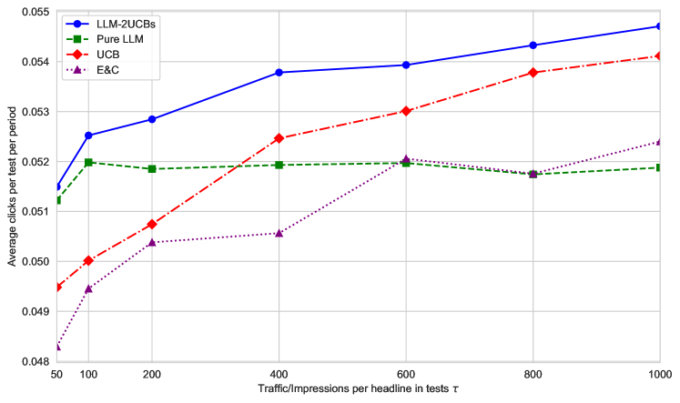
Figure 10: Average clicks per experiment per period under different time horizon multipliers. Note that the Y-axis captures the average clicks per test per period. For instance, if there is a test with two headlines conducted under $x=100$, then the average click per period in this test is calculated as $(1+2)/100=0.03$. The Y value is simply the average of this number $0.03$ over all tests. This measure scales well with the platform’s total clicks in tests because headlines in different tests with different numbers of headlines take the same weight in this measure.

Parameter $\tau$	LLM-2UCBs vs Pure LLM	LLM-2UCBs vs UCB	LLM-2UCBs vs E&C	Pure LLM vs UCB	Pure LLM vs E&C	UCB vs E&C
50	$0.53$	$4.06$∗	$6.63$∗∗∗∗	$3.52$∗	$6.07$∗∗∗	$2.46$
100	$1.04$∗	$5.01$∗∗∗∗	$6.20$∗∗∗∗	$3.93$∗∗	$5.11$∗∗∗∗	$1.13$
200	$1.92$∗∗∗∗	$4.14$∗∗∗∗	$4.89$∗∗∗∗	$2.18$∗	$2.92$∗∗	$0.72$
400	$3.57$∗∗∗∗	$2.51$∗∗∗	$6.36$∗∗∗∗	$-1.02$	$2.70$∗∗∗	$3.76$∗∗∗∗
600	$3.78$∗∗∗∗	$1.74$∗∗	$3.60$∗∗∗∗	$-1.96$∗∗	$-0.17$	$1.83$∗∗∗
800	$5.00$∗∗∗∗	$1.02$∗	$4.97$∗∗∗∗	$-3.79$∗∗∗∗	$-0.03$	$3.91$∗∗∗∗
1000	$5.46$∗∗∗∗	$1.10$∗	$4.41$∗∗∗∗	$-4.13$∗∗∗∗	$-1.00$	$3.27$∗∗∗∗

Table 7: Percentage % reward improvement between two algorithms with significance levels: ^∗ $p\leq$ 0.05, ^∗∗ $p\leq$ 0.01, ^∗∗∗ $p\leq$ 0.001, ^∗∗∗∗ $p\leq$ 0.0001. For example, under the impression per headline equal to 50, the average click per test of LLM-2UCBs and Pure LLM is 0.05149 and 0.05122, respectively; so the relative improvement is calculated as ${0.05149}/{0.05122}-1=0.53\%$. Parameter $\tau$ represents the average impression per headline to scale the time horizon $T=\tau\times K$.

5 Conclusion

We note that our approach is quite general and is agnostic to the exact nature of the LLM-based approach used. Thus, any of the LLM-based approaches discussed in Section 3 can be used in the first step of our approach. This is important since the LLM models and fine-tuning approaches continue to advance quickly; so the plug-and-play nature of our approach extends well to this setting. In addition, when considering personalization and accessing contextual information (e.g., readers’ features), we can incorporate this extra information as inputs to the LLM-based CTR prediction model and integrate it into contextual bandit algorithms. Specifically, we provide two variants of LOLA for this purpose in Web Appendix B.

In conclusion, our study introduces LOLA, a novel framework that combines the predictive power of LLMs with the adaptive efficiency of online learning algorithms to enhance content experimentation. By leveraging LLM-based prediction models as priors, our approach minimizes regret in real time, leading to significant improvements in total reward/clicks. Furthermore, through the numerical analysis based on a large-scale dataset from Upworthy, we demonstrate that LOLA outperforms traditional A/B testing and pure online learning algorithms, particularly in settings with limited experimental traffic or a large number of arms. These conditions are prevalent in the current content industry, where platform users can easily create and share their content, such as on platforms like X and TikTok. Our numerical results also indicate that while LLMs provide valuable predictions, one cannot fully trust the prediction results solely from LLMs since experimentation-based approaches still remain the gold standard and can be leveraged to correct the errors in LLMs.

From a managerial perspective, LOLA offers a versatile solution applicable to various scenarios where firms need to decide on content display, such as news articles, headlines, advertisements, or website content. Utilizing open-source LLM models, this method is cost-effective and can be easily deployed across different tasks once LLM models are fine-tuned on relevant datasets. The fine-tuning process is cost-efficient and can be performed on entry-level GPUs, making advanced LLM-based techniques accessible to firms with limited budgets. Additionally, we document that prompt-based approaches, which have been the standard method in recent marketing literature, perform poorly in this content attractiveness comparison task, underscoring the importance of the fine-tuning approach.

Finally, we highlight that LOLA can be readily adapted to other measures beyond clicks. The click-based metric, while widely used by Upworthy a decade ago, has raised concerns about promoting clickbait headlines, which may reduce user engagement or spread negativity. The industry is rapidly evolving, with Upworthy now focusing more on content quality and humanity, although clicks still remain an important measure; see more detailed discussion in (Upworthy2023). Our LOLA framework can easily accommodate these changes by adjusting the reward notion in the algorithm to align with new business goals, demonstrating its flexibility and relevance in a dynamic industry.

Code and Data

The code used in this study is publicly available at LLM News Github Repository to enable the reproduction of our results and to support future research that applies LLMs to experimentation and business problems.

Funding and Competing Interests Declaration

Author(s) have no competing interests to declare.

Appendix A Supplementary Materials for Section 3

A.1 Pairwise Comparison Between GPT Prompts

To determine whether one prompt is significantly better than the other, we record a binary indicator of the correct/incorrect answer for each prompt on each sample and then conduct a paired t-test on 1,000 correct/incorrect answer indicators to see whether the answers from one prompt are significantly more accurate than the other. The mean differences and p values are documented in Figure A1 and Figure A2. The random guess model simply predicts the first headline wins with a half probability. The nomenclature for GPT prompts in these two figures follows a specific format. The first component is the name of the GPT model, the second component indicates the number of demonstrations, and the third component specifies whether the outputs in the demonstrations are flipped. A value of 0 indicates the correct label, while a value of 1 indicates the wrong label. For example, GPT-4-0-0 means zero-shot prompting using GPT-4, and GPT-3.5-5-1 means in-context learning with 5 demonstrations and wrong labels using GPT-3.5.

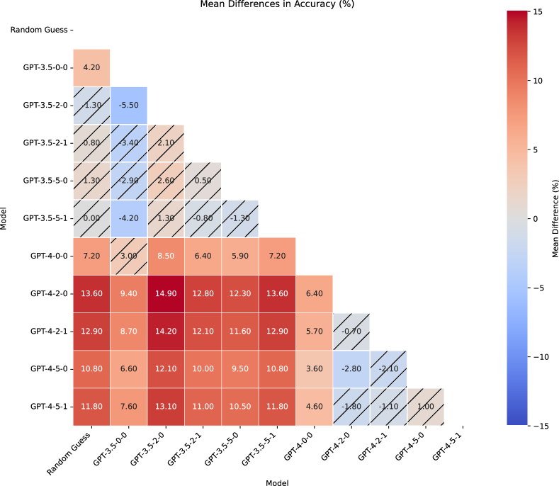
Figure A1: Average accuracy differences between different GPT prompts. The number in the heatmap presents the accuracy of prompts indicated on the left minus the accuracy of prompts indicated at the bottom. Shaded blocks indicate insignificant differences.

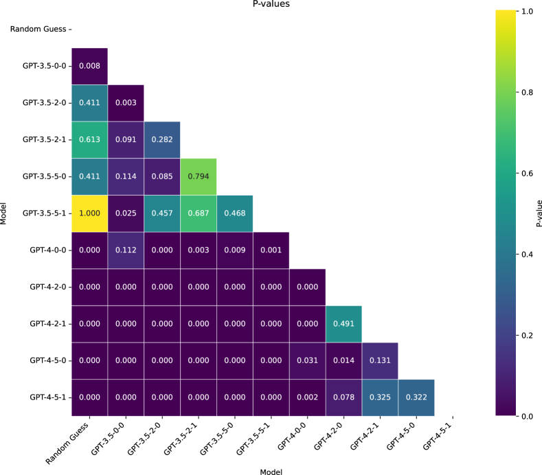
Figure A2: The number in the heatmap presents the p-value from the paired t-test between different GPT prompts.

A.2 Implementation Details of MLP Classification Models

Hyperparameters of the network structure. We employ a fully connected neural network with ReLU activation functions for the hidden layers and a sigmoid activation function for the output layer. This configuration is widely used in practice. To determine the number of layers and the hidden nodes of each layer, we choose the number of layers within the range of $\{1,2,3,4,5\}$, and set the number of nodes in the first fully connected layer from the set $\{128,256,512,1024,2048\}$. Besides, we adjust the previous-post ratio, which is the proportion of nodes in each layer relative to those in the subsequent layer. This ratio here is in $\{2,4,8\}$. Note that the previous-post ratio becomes irrelevant to the results when there’s only one hidden layer. This is because the final output layer has only one dimension for ranking the most attractive headline. We incorporate the dropout after each hidden layer to mitigate the overfitting. Dropout layers randomly deactivate neurons based on a specified dropout rate, while scaling up the remaining neurons to maintain the same mean of the layer. In this work, we set the dropout rate in $\{0.3,0.5\}$. All hyperparameters are automatically selected through hyperparameter optimization, which is introduced below.

Hyperparameters of the training procedure. The MLP is implemented in PyTorch, with data split into 70% for training, 10% for validation, and 20% for testing. To prevent the network from memorizing the order of samples, we shuffle the training set at the start of each epoch. Determining the appropriate batch size is crucial, as large batch sizes may lead to convergence to local optima, while small batch sizes may hinder convergence. We balance accuracy and training speed by setting the batch size to 10 and the learning rate to $0.01$. Additionally, to mitigate overfitting, we apply $L_{2}$ regularization, with the regularization weight chosen from $\{1e-6,1e-4,1e-2\}$. We use binary cross-entropy as the loss function and employ stochastic gradient descent for training. We implement early stopping by monitoring the validation set loss, halting the training process if the reduction in loss over 60 epochs falls below a tolerance threshold of $10^{-4}$.

Hyperparameter optimization. We optimize the parameters mentioned above through Bayesian Optimization (snoek2012practical). This Bayesian technique uses Bayesian inference to construct a probabilistic model of the objective function, where the parameters are updated iteratively with new observations. This iterative process balances exploration of the parameter space to discover promising regions and exploitation of known high-performing areas. In this work, we consider the accuracy of the validation set as the objective and optimize hyperparameters selected from the specified parameter space, as delineated by the ranges mentioned previously. We choose the Gaussian process as the estimator with the automatic optimizer, which is commonly adopted by the community. To ensure a judicious trade-off between efficacy and efficiency, we repeat the optimization process 50 times for input data of 256 dimensions and 30 times for data of 3,072 dimensions.

A.3 Results of DistilBERT LoRA Fine-Tuning

One difference between DistilBERT and Llama-3 is that DistilBERT is a bidirectional Transformer model, which means that its attention mechanism allows the model to learn the context from both directions, while Llama-3 is a unidirectional model. An illustration of the structure of the DistilBERT model combined with a classification head is shown in Figure A3. By default, DistilBERT can handle two headlines together as input. The format of the input is: [CLS] Headline 1 [EOS] Headline 2 [EOS]. The [CLS] token is a special token used to get the output of the model for classification, and the output of the last Transformer layer corresponding to this token is used as the input to the classification head. The [EOS] token is used to separate the two sentences.

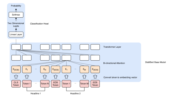
Figure A3: The classification pipeline using the DistilBERT model. Headlines are first tokenized, and each token is converted into an embedding vector. For illustrative purposes, only two Transformer layers are shown. The figure highlights the use of bidirectional attention in DistilBERT, whereby each token can incorporate information from any token. Connections between Transformer blocks represent the attention mechanism, and only a subset of these links are displayed for simplicity. The output from the first token (CLS token) is fed into a classification head, which computes the probability that one headline is more impactful than the other.

Another difference is that DistilBERT is a smaller model compared to Llama-3-8b. DistilBERT has around 66 million parameters, which is only 0.94% of the parameters of Llama-3-8b. Due to the smaller model size, we are able to conduct full parameter updates during the fine-tuning process without using LoRA. We use the same learning rate scheduling, number of training epochs, and train-test set split as in the experiment detailed in Section 3.3.3. The accuracy of DistilBERT LoRA fine-tuning on the same test set is around 75%. More details can be found in the code repository.

Appendix B Algorithms with Contextual Information

For the completeness of the paper, we introduce two additional LOLA algorithms in this appendix, which leverage contextual information.

For linear contextual bandits, we assume that at each round, we first observe the context vector $x_{t,k}\in\mathbb{R}^{d}$ for each arm $k\in[K]$. This context information can include LLM embedding vectors and user information, among other features. We denote by $r_{t,k}$ the random reward of arm $k$ at round $t$. After pulling one arm at each round, only the reward of that arm, $r_{t}$, is revealed. We make the linear realizability assumption that the expected reward is linear in the context vectors, which means $\mathbb{E}[r_{t,k}|x_{t,k}]=x_{t,k}^{\top}\theta^{*}$. The weight vector $\theta^{*}\in\mathbb{R}^{d}$ is unknown and needs to be learned. Additionally, we assume access to a historical dataset of size $M$, denoted by $\{(x_{t,k},r_{t})\}_{t=-M}^{-1}$. With these definitions, we are ready to present our proposed Algorithm 2, named LLM-Assisted Linear Contextual Bandit. The LLM-LinUCB algorithm extends LinUCB (chu2011contextual). Under the linear realizability assumption, this algorithm achieves asymptotically optimal regret, matching the lower bound up to logarithmic factors.

Algorithm 2 LLM-Assisted Linear Contextual Bandit (LLM-LinUCB)

1:LLM Training Phase: Calculate $A\leftarrow I_{d}+\sum_{t=-M}^{-1}x_{t,a_{t}}x_{t,a_{t}}^{\top}$ (The $d$-by-$d$ identity matrix), and $b\leftarrow\sum_{t=-M}^{-1}x_{t,a_{t}}r_{t}$

2:Hyperparameter Fine Tune: $\alpha\in\mathbb{R}^{+}$ for controlling the upper bound.

3:Online Learning Phase: Initialize the number of periods $T$, number of arms $K$.

4:for $t=1$ to $T$ do

5:     Get weight estimator: $\theta_{t}\leftarrow A^{-1}b$

6:     Observe $K$ context vectors, $x_{t,1},x_{t,2},\dots,x_{t,K}\in\mathbb{R}^{d}$, generated through an LLM-based embedding model concatenated with user context information.

7:     for $k=1,2,\dots,K$ do

8:         $\hat{r}_{t,k}\leftarrow\theta_{t}^{\top}x_{t,k}+\alpha\sqrt{x_{t,k}^{\top}A^{-1}x_{t,k}}$ (Computes the upper confidence bound)

9:     end for

10:     Choose action $a_{t}=\arg\max_{k\in[K]}\hat{r}_{t,k}$.

11:     Observe reward $r_{t}$.

12:     $A\leftarrow A+x_{t,a_{t}}x_{t,a_{t}}^{\top}$.

13:     $b\leftarrow b+x_{t,a_{t}}r_{t}$.

14:end for

The algorithm proceeds as follows: During the LLM training phase, we prepare the matrix $A$ and vector $b$ to estimate the linear weight vector. We may need an LLM-based embedding model to extract embedding vectors from the original text information. Similar to LLM-2UCBs, we fine-tune the upper bound control parameter $\alpha$ using another fold of data and a bisection search to minimize regret on this fine-tuning dataset. The online learning phase remains the same as the standard LinUCB.

The advantages of LLM-LinUCB are its transparency due to the linear assumption, ease of execution with only one hyperparameter, and theoretical soundness with optimal regret. However, it is restricted to linear forms. There are two issues with this assumption. First, although we have shown that linear functions almost fully leverage text embeddings from OpenAI to achieve high accuracy (there is almost no difference compared to MLP), the embedding itself sacrifices a lot of information, as demonstrated by the significant outperformance of LoRA fine-tuning over embedding-based classification. Second, once concatenated with user contexts, it is unclear whether the linear form is a good approximation, necessitating further numerical study.

To alleviate the limitations of the linear assumption, we introduce another LLM-assisted contextual bandit algorithm (Algorithm 3), which extends the FAst Least-squares-regression-oracle CONtextual bandits (FALCON) algorithm proposed by (simchi2022bypassing). This type of contextual bandit algorithm generalizes the linear realizability assumption to a more flexible framework, assuming the true prediction model $f^{*}\in\mathcal{F}$. The functional class $\mathcal{F}$ can be very general and is not limited to linear models. This assumption is reasonable and promising because LLMs have demonstrated their capability across a wide range of tasks. Essentially, $\mathcal{F}$ can be viewed as a class of LLM models, and the goal is to find the true LLM model $f^{*}$ that performs best for our task, i.e., $f^{*}(x_{t,k},k)=\mathbb{E}[r_{t,k}|x_{t,k}]$ for any $k\in[K]$ and $x_{t,k}\in\mathcal{X}$. Under this setting, the context information is not restricted to real numbers and can include more general data, such as text information. We now present the LLM-FALCON algorithm.

Algorithm 3 LLM-Assisted FAst Least-squares-regression-oracle CONtextual bandits (LLM-FALCON)

1:LLM Training Phase: Obtain the historical data $\{(x_{t,k},r_{t})\}_{t=-M}^{0}$, and construct an LLM $\mathcal{F}$ class for training.

2:Hyperparameter Fine Tuning: Confidence control parameter $\delta$.

3:Online Learning Phase: Initialize $T$, $K$, and the epoch schedule $0=\tau_{0}<\tau_{1}<\tau_{2}<\cdots$.

4:for epoch $m=1,2,\dots$ do

5:     Set $\gamma_{m}=(1/30)\sqrt{(K\tau_{m-1})/\log(|\mathcal{F}|\tau_{m-1}/\delta)}$ (for epoch 1, $\gamma_{1}=1$).

6:     Compute $\hat{f}_{m}=\arg\min_{f\in\mathcal{F}}\sum_{t=-M}^{\tau_{m-1}}(f(x_{t,a_{t}},a_{t})-r_{t})^{2}$ via the offline least squares oracle.

7:     for round $t=\tau_{m-1}+1,\dots,\tau_{m}$ do

8:         Observe contexts $x_{t,k}\in\mathcal{X}$,$\forall k\in[K]$.

9:         Compute $\hat{f}_{m}(x_{t,k},k)$ for each arm $k\in[K]$. Let $\hat{a}_{t}=\arg\max_{k\in[K]}\hat{f}_{m}(x_{t,k},k)$.

10:         Define

$$p_{t}(k)=\begin{cases}\frac{1}{K+\gamma_{m}(\hat{f}_{m}(x_{t,\hat{a}_{t}},\hat{a}_{t})-\hat{f}_{m}(x_{t,k},k))},&\forall k\neq\hat{a}_{t},\\ 1-\sum_{k\neq\hat{a}_{t}}p_{t}(k),&k=\hat{a}_{t}.\end{cases}$$

11:         Sample $a_{t}\sim p_{t}(\cdot)$ and observe reward $r_{t}$.

12:     end for

13:end for

At the beginning of each epoch, we retrain the LLM using all available data up to that point, as detailed in Line 6. For simplicity, this algorithm assumes no optimization error during training, utilizing the offline least squares oracle instead. However, in practice, achieving zero optimization error is impossible, and one can incorporate this error into the final regret term using the regret triangle decomposition. Although this algorithm can handle original text information and fits into a general LLM model (not restricted to linear models), the primary challenge is the cost of training the LLM at each epoch because training a full LLM is typically time-consuming and costly. One potential solution, as investigated in our paper, is to fine-tune the LLM using LoRA instead of fully retraining it with new data. However, the empirical performance of this method remains unclear.

After getting an LLM trained on new data, then the key step in this algorithm is using the “inverse proportional to the gap” rule to balance exploration and exploitation. At each round, we first identify the empirically best arm $\hat{a}_{t}$ and then compute the gap in expected reward between this arm and the others. The sampling probability $p_{t}(k)$ is inversely proportional to this gap, meaning that a larger estimated reward $\hat{f}_{m}(x_{t,k},k)$ results in a smaller gap and a higher probability of being pulled. For a more detailed discussion of this algorithm, please refer to (simchi2022bypassing). Our purpose here is to adapt this algorithm in the LLM setting and discuss its pros and cons for completeness.

Appendix C LLM-Assisted Thompson Sampling

For completeness, we also present another version of LOLA that combines LLM and Thompson Sampling. We will update its numerical results in the next version of the manuscript.

Algorithm 4 LLM-Assisted Thompson Sampling (LLM-TS)

1:LLM Training Phase: Train a LLM-based prediction model $\mathcal{M}(x)$ for CTRs using historical data samples, where $x$ is the contextual information for arms.

2:Hyperparameter Fine-Tuning: Use another subset of data to select the LLM’s equivalent auxiliary sample size, $n^{\text{a}ux}$ and the standard TS prior $(\alpha^{0},\beta^{0})$.

3:Online Learning Phase: Initialize the number of periods $T$, number of arms $K$, LLM-based CTR prediciton $\bar{\mu}^{\text{a}ux}_{k}\leftarrow\mathcal{M}(x_{k})$, the parameters in Beta priors $(\alpha^{1}_{k},\beta^{1}_{k})\leftarrow(\alpha^{0},\beta^{0})+(n^{\text{a}ux}\bar{\mu}^{\text{a}ux}_{k},n^{\text{a}ux}(1-\bar{\mu}^{\text{a}ux}_{k}))$ for all arms $k\in[K]$.

4:for $t=1$ to $T$ do

5:     Sample $\theta_{k}^{t}\sim\text{beta}(\alpha^{t}_{k},\beta^{t}_{k})$ for all arms $k\in[K]$.

6:     Play the arm $a_{t}=\arg\max_{k\in[K]}\theta_{k}^{t}$.

7:     Observe the payoff $r_{a_{t}}$.

8:     Update $(\alpha^{t+1}_{k},\beta^{t+1}_{k})\leftarrow(\alpha^{t}_{k},\beta^{t}_{k})+(r_{a_{t}},1-r_{a_{t}})$ if $a_{t}=k$; update $(\alpha^{t+1}_{k},\beta^{t+1}_{k})\leftarrow(\alpha^{t}_{k},\beta^{t}_{k})$ if $a_{t}\neq k$.

9:end for

Appendix D Survey Results

To illustrate the difficulty of the headline selection task and compare it with LLM-based methods, we conducted a survey among students, asking respondents which headline was catchier.

Specifically, we conducted the survey study among undergraduate students, acknowledging that these participants were less experienced in editing than Upworthy editors and writers. Despite this limitation, we aim to highlight the challenges of this task for humans. It is important to note that all candidate headlines were chosen by Upworthy editors, who were uncertain which one was catchier, prompting the need for further A/B testing.

We designed two similar surveys using Qualtrics. The first survey randomly sampled 3,000 pairs from 39,158 headline pairs, differentiated by CTRs at a 0.05 significance level, along with 500 pairs showing no significant differences in CTRs. The second survey utilized the same 3,000 significant samples as the first. In both surveys, students were asked to select the catchier headline from each pair. The introductory text for the surveys was:
“Please help us understand what makes a news headline appealing to readers. In this survey, you will be presented with 20 pairs of headlines. Please choose the one that captures your attention more effectively or feels more engaging in each pair, assuming both headlines relate to the same news content. There are no right or wrong answers; we are simply interested in your opinions.”
After providing identification information, including the last four digits of their phone and student ID, respondents proceeded to a new page featuring 20 headline comparison questions with the prompt, “Please select the headline that you find more attractive,” with only one permissible response. Notably, the first survey included an additional response option: “Both headlines seem equally good.” At the survey’s conclusion, we asked, “How often do you read the news?” with options “Never”, “1-2 days per week”, “3-4 days per week”, “5-6 days per week”, “Everyday”.

Detailed information and survey results are recorded in Table A1. Because some students did not finish the survey or skipped some comparisons, one can see there are 3,809 responses out of $202\times 20=4,040$. To calculate the accuracy metric, we only focused on the significant pairs, and in the first survey, we ruled out the uncertain answer “Both headlines seem equally good” for a relatively fair comparison between the two surveys. “Accuracy” measure here is consistent with the LLM tests. We viewed the headline with a higher CTR as the correct answer, and calculated the proportion of correct answers as accuracy. By doing so, one should expect 50% accuracy by random guess since we randomly swapped the order of the headlines to make sure the displayed order does not correlate with the correct answer.

Detailed information and survey results are documented in Table A1. Some students did not complete the survey or skipped some comparisons, resulting in 3,809 responses out of a potential 4,040 ($202\times 20$). To calculate the accuracy metric, we focused solely on the significant pairs, and in the first survey, we excluded the uncertain answer “Both headlines seem equally good” to facilitate a fair comparison between the two surveys. Accuracy here aligns with the LLM tests. We regarded the headline with the higher CTR as the correct answer and calculated the proportion of correct responses as accuracy. Accordingly, one might expect a 50% accuracy rate from random guessing, as we randomized the order of the headlines to ensure that the display order did not correlate with the correct answer.

The survey results indicate that respondents’ ability to identify catchier headlines is comparable to random guessing, with no accuracies significantly deviating from 50% at the 0.05 significance level. Furthermore, accuracies did not vary significantly across different groups based on news reading frequency. We also incorporated two attention checks in the second survey. These findings suggest that the human ability to discern catchier headlines is limited, highlighting the intrinsic difficulty of the task.

		Survey 1	Survey 2
conducted time		4/14 - 4/21	4/29 - 5/17
# of respondents		202	339
headline pair pool		3000 significant + 500 insignificant pairs	3000 significant pairs
# of sampled pairs in survey		20	20
# total received responses		3,809	4,571
overall accuracy %		45.22	51.58
	Results based on different answer to “How often do you read the news?”
Never	proportion %	21.78	16.22
	accuracy %	45.76	51.62
1-2 days per week	proportion %	48.51	49.56
	accuracy %	45.36	52.54
3-4 days per week	proportion %	18.81	18.29
	accuracy %	46.83	51.39
5-6 days per week	proportion %	4.95	5.31
	accuracy %	39.05	50.15
Everyday	proportion %	5.94	8.26
	accuracy %	42.35	47.48

Table A1: Survey Response Analysis. No accuracies in this table are significantly lower or higher than 50% at 0.05 significant level. 8 respondents did not finish Survey 2 in the limited given time, so the summation of proportion from different subgroups is smaller than 100% in Survey 2.

References

- Ainslie et al. (2023) Joshua Ainslie, James Lee-Thorp, Michiel de Jong, Yury Zemlyanskiy, Federico Lebrón, and Sumit Sanghai. Gqa: Training generalized multi-query transformer models from multi-head checkpoints. arXiv preprint arXiv:2305.13245, 2023.
- Ba et al. (2016) Jimmy Lei Ba, Jamie Ryan Kiros, and Geoffrey E Hinton. Layer normalization. arXiv preprint arXiv:1607.06450, 2016.
- Chu et al. (2011) Wei Chu, Lihong Li, Lev Reyzin, and Robert Schapire. Contextual bandits with linear payoff functions. In Proceedings of the Fourteenth International Conference on Artificial Intelligence and Statistics, pages 208–214. JMLR Workshop and Conference Proceedings, 2011.
- Coenen (2019) Anna Coenen. How The New York Times is experimenting with recommendation algorithms. NYT Open, 2019. URL {https://open.nytimes.com/how-the-new-york-times-is-experimenting-with-recommendation-algorithms-562f78624d26}. Accessed: 2024-05-24.
- Devlin et al. (2018) Jacob Devlin, Ming-Wei Chang, Kenton Lee, and Kristina Toutanova. Bert: Pre-training of deep bidirectional transformers for language understanding. arXiv preprint arXiv:1810.04805, 2018.
- Garg et al. (2022) Shivam Garg, Dimitris Tsipras, Percy S Liang, and Gregory Valiant. What can transformers learn in-context? A case study of simple function classes. Advances in Neural Information Processing Systems, 35:30583–30598, 2022.
- Gur and Momeni (2022) Yonatan Gur and Ahmadreza Momeni. Adaptive sequential experiments with unknown information arrival processes. Manufacturing & Service Operations Management, 24(5):2666–2684, 2022.
- He et al. (2016) Kaiming He, Xiangyu Zhang, Shaoqing Ren, and Jian Sun. Deep residual learning for image recognition. In Proceedings of the IEEE conference on computer vision and pattern recognition, pages 770–778, 2016.
- Houlsby et al. (2019) Neil Houlsby, Andrei Giurgiu, Stanislaw Jastrzebski, Bruna Morrone, Quentin De Laroussilhe, Andrea Gesmundo, Mona Attariyan, and Sylvain Gelly. Parameter-efficient transfer learning for nlp. In International conference on machine learning, pages 2790–2799. PMLR, 2019.
- Hu et al. (2021) Edward J Hu, Yelong Shen, Phillip Wallis, Zeyuan Allen-Zhu, Yuanzhi Li, Shean Wang, Lu Wang, and Weizhu Chen. Lora: Low-rank adaptation of large language models. arXiv preprint arXiv:2106.09685, 2021.
- Kusupati et al. (2022) Aditya Kusupati, Gantavya Bhatt, Aniket Rege, Matthew Wallingford, Aditya Sinha, Vivek Ramanujan, William Howard-Snyder, Kaifeng Chen, Sham Kakade, Prateek Jain, et al. Matryoshka representation learning. Advances in Neural Information Processing Systems, 35:30233–30249, 2022.
- Lattimore and Szepesvári (2020) Tor Lattimore and Csaba Szepesvári. Bandit algorithms. Cambridge University Press, 2020.
- Li et al. (2010) Lihong Li, Wei Chu, John Langford, and Robert E Schapire. A contextual-bandit approach to personalized news article recommendation. In Proceedings of the 19th international conference on World wide web, pages 661–670, 2010.
- Li et al. (2024) Peiyao Li, Noah Castelo, Zsolt Katona, and Miklos Sarvary. Frontiers: Determining the validity of large language models for automated perceptual analysis. Marketing Science, 2024.
- Li and Liang (2021) Xiang Lisa Li and Percy Liang. Prefix-tuning: Optimizing continuous prompts for generation. arXiv preprint arXiv:2101.00190, 2021.
- Matias et al. (2021) J Nathan Matias, Kevin Munger, Marianne Aubin Le Quere, and Charles Ebersole. The upworthy research archive, a time series of 32,487 experiments in us media. Scientific Data, 8(1):195, 2021.
- Meta-AI (2024) Meta-AI. Introducing meta-llama 3, 2024. URL https://ai.meta.com/blog/meta-llama-3.
- Meta-Llama (2024) Meta-Llama. LLAMA3 model card, 2024. URL https://github.com/meta-llama/llama3/blob/main/MODEL_CARD.md.
- Min et al. (2022) Sewon Min, Xinxi Lyu, Ari Holtzman, Mikel Artetxe, Mike Lewis, Hannaneh Hajishirzi, and Luke Zettlemoyer. Rethinking the role of demonstrations: What makes in-context learning work? arXiv preprint arXiv:2202.12837, 2022.
- OpenAI (2024) OpenAI. New embedding models and api updates, 2024. URL https://openai.com/index/new-embedding-models-and-api-updates/. Accessed: 2024-05-28.
- Patil et al. (2023) Rajvardhan Patil, Sorio Boit, Venkat Gudivada, and Jagadeesh Nandigam. A survey of text representation and embedding techniques in NLP. IEEE Access, 2023.
- Reimers and Gurevych (2019) Nils Reimers and Iryna Gurevych. Sentence-bert: Sentence embeddings using siamese bert-networks. arXiv preprint arXiv:1908.10084, 2019.
- Reneau (2023) Annie Reneau. Study of upworthy headlines claims negativity drives website clicks. We have some thoughts. Upworthy, 2023. URL https://www.upworthy.com/upworthy-negative-headlines-study. Accessed: 2024-05-24.
- Sanh et al. (2019) Victor Sanh, Lysandre Debut, Julien Chaumond, and Thomas Wolf. Distilbert, a distilled version of bert: smaller, faster, cheaper and lighter. arXiv preprint arXiv:1910.01108, 2019.
- Saunshi et al. (2020) Nikunj Saunshi, Sadhika Malladi, and Sanjeev Arora. A mathematical exploration of why language models help solve downstream tasks. arXiv preprint arXiv:2010.03648, 2020.
- Schwartz et al. (2017) Eric M Schwartz, Eric T Bradlow, and Peter S Fader. Customer acquisition via display advertising using multi-armed bandit experiments. Marketing Science, 36(4):500–522, 2017.
- Shazeer (2020) Noam Shazeer. Glu variants improve transformer. arXiv preprint arXiv:2002.05202, 2020.
- Simchi-Levi and Xu (2022) David Simchi-Levi and Yunzong Xu. Bypassing the monster: A faster and simpler optimal algorithm for contextual bandits under realizability. Mathematics of Operations Research, 47(3):1904–1931, 2022.
- Su et al. (2024) Jianlin Su, Murtadha Ahmed, Yu Lu, Shengfeng Pan, Wen Bo, and Yunfeng Liu. Roformer: Enhanced transformer with rotary position embedding. Neurocomputing, 568:127063, 2024.
- Symonds (2017) Alexandria Symonds. When a headline makes headlines of its own. The New York Times, 2017. URL {https://www.nytimes.com/2017/03/23/insider/headline-trump-time-interview.html}. Accessed: 2024-05-24.
- Vaswani et al. (2017) Ashish Vaswani, Noam Shazeer, Niki Parmar, Jakob Uszkoreit, Llion Jones, Aidan N Gomez, Łukasz Kaiser, and Illia Polosukhin. Attention is all you need. Advances in neural information processing systems, 30, 2017.
- Xie and Min (2022) Sang Michael Xie and Sewon Min. How does in-context learning work? A framework for understanding the differences from traditional supervised learning. SAIL Blog, 2022. URL {http://ai.stanford.edu/blog/understanding-incontext/}.
- Xie et al. (2021) Sang Michael Xie, Aditi Raghunathan, Percy Liang, and Tengyu Ma. An explanation of in-context learning as implicit bayesian inference. arXiv preprint arXiv:2111.02080, 2021.
- Yang (2024) Kathy Yang. Milestones on our journey to standardize experimentation at The New York Times. NYT Open, 2024. URL {https://open.nytimes.com/milestones-on-our-journey-to-standardize-experimentation-at-the-new-york-times-2c6d32db0281}. Retrieved: 2024-05-24.
- Yoganarasimhan and Yakovetskaya (2024) Hema Yoganarasimhan and Irina Yakovetskaya. From feeds to inboxes: A comparative study of polarization in facebook and email news sharing. Management Science, forthcoming, 2024.
- Zaken et al. (2021) Elad Ben Zaken, Shauli Ravfogel, and Yoav Goldberg. Bitfit: Simple parameter-efficient fine-tuning for transformer-based masked language-models. arXiv preprint arXiv:2106.10199, 2021.
- Zhang et al. (2021) Aston Zhang, Zachary C Lipton, Mu Li, and Alexander J Smola. Dive into deep learning. arXiv preprint arXiv:2106.11342, 2021.
- Zhang and Sennrich (2019) Biao Zhang and Rico Sennrich. Root mean square layer normalization. Advances in Neural Information Processing Systems, 32, 2019.
- Zhao et al. (2024) Justin Zhao, Timothy Wang, Wael Abid, Geoffrey Angus, Arnav Garg, Jeffery Kinnison, Alex Sherstinsky, Piero Molino, Travis Addair, and Devvret Rishi. Lora land: 310 fine-tuned llms that rival gpt-4, a technical report. arXiv preprint arXiv:2405.00732, 2024.
- Zhou et al. (2024) Zixuan Zhou, Xuefei Ning, Ke Hong, Tianyu Fu, Jiaming Xu, Shiyao Li, Yuming Lou, Luning Wang, Zhihang Yuan, Xiuhong Li, et al. A survey on efficient inference for large language models. arXiv preprint arXiv:2404.14294, 2024.

References

- Chu et al. (2011) Wei Chu, Lihong Li, Lev Reyzin, and Robert Schapire. Contextual bandits with linear payoff functions. In Proceedings of the Fourteenth International Conference on Artificial Intelligence and Statistics, pages 208–214. JMLR Workshop and Conference Proceedings, 2011.
- Simchi-Levi and Xu (2022) David Simchi-Levi and Yunzong Xu. Bypassing the monster: A faster and simpler optimal algorithm for contextual bandits under realizability. Mathematics of Operations Research, 47(3):1904–1931, 2022.
- Snoek et al. (2012) Jasper Snoek, Hugo Larochelle, and Ryan P Adams. Practical bayesian optimization of machine learning algorithms. Advances in neural information processing systems, 25, 2012.